Learning enhanced model reference adaptive control algorithms via a cost-effective educational plant

Abstract

The enhanced model reference adaptive control (EMRAC) strategy is an effective extension of the model reference adaptive control (MRAC) algorithm, designed to steer the trajectories of plants towards those of a reference model despite uncertain plant parameters, unknown nonlinear dynamics, and disturbances by adapting the control gains in operation. However, MRAC algorithms are usually taught only in advanced control engineering courses, as they are more complex compared to linear control methods. To demonstrate the potential of EMRAC solutions for controlling systems with limited knowledge of plant dynamics and to facilitate students’ learning, this article presents the control formulation, design, and experimental validation of EMRAC strategies for an educational plant (i.e., the speed control of a DC motor through Arduino). Despite being modelled as a first order system, this plant is characterised by system nonlinearities and parameter uncertainties which can jeopardise closed-loop tracking performance of a controller with fixed gains. An incremental approach is used to introduce the EMRAC algorithm, with only knowledge in linear control design, e.g., pole-placement methods, assumed as a prerequisite. Specifically, the need for MRAC strategies is first introduced as a possible solution to overcome limitations of pole-placement techniques by adapting the control gains. Then, the classical MRAC strategy, along with methods for limiting the growth of the gains, is reviewed, and finally, two EMRAC strategies are presented. The improved closed-loop tracking performance given by the EMRAC strategies are also assessed quantitatively and compared to those obtained with two linear control solutions and two classical MRAC methods.

Introduction

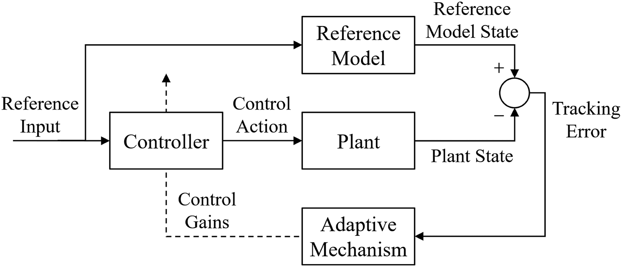
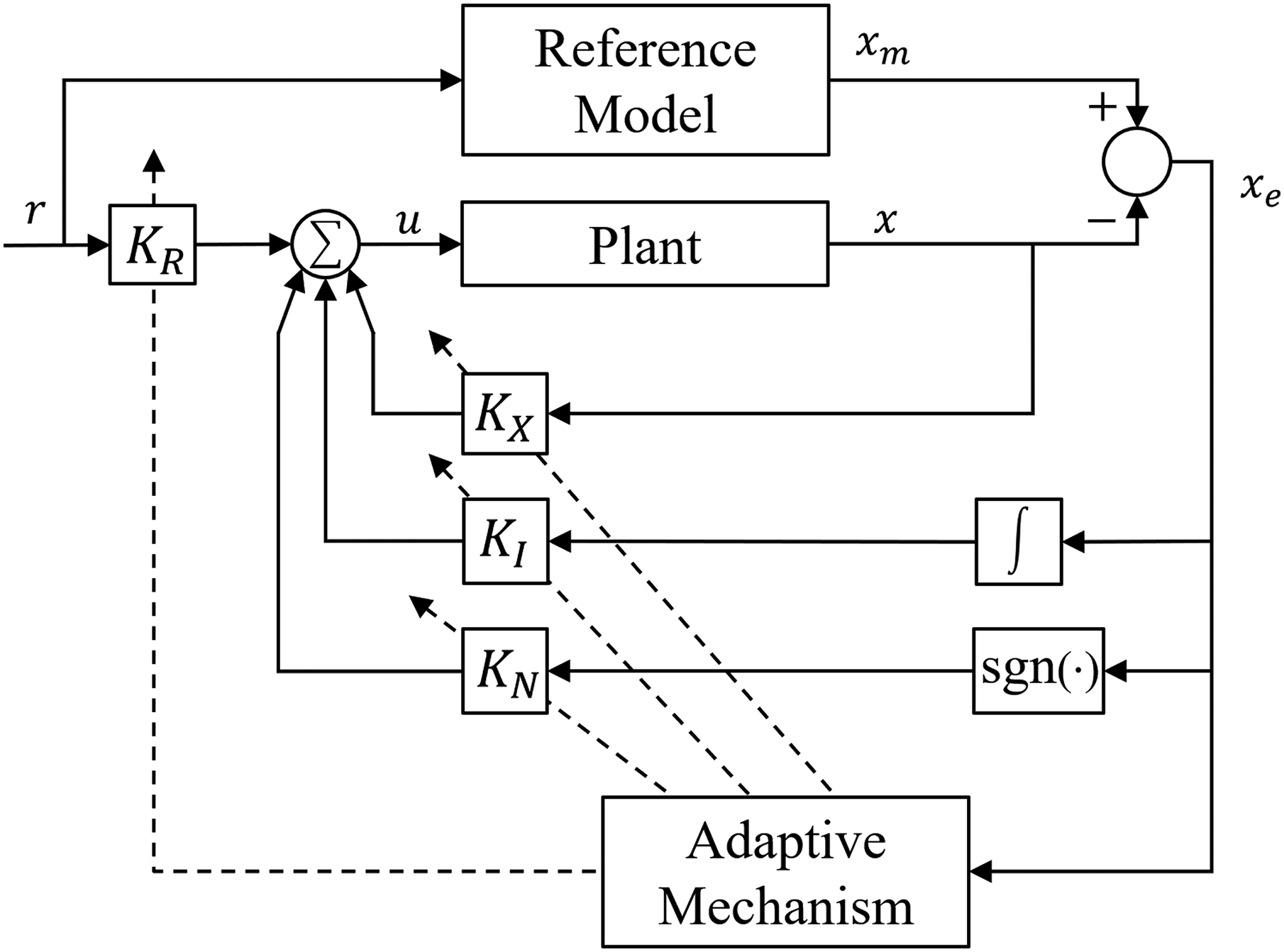
Adaptive control emerged in the early 1950s with the aim of controlling the dynamics of systems with significant parametric uncertainty and high variability. ¹ Within this framework, model reference adaptive control (MRAC) is an effective design method to control engineering plants with unknown parameters. In the MRAC formulations, control specifications (e.g., closed-loop step response parameters, such as settling time) are embedded into the design of a reference model that describes the ideal behaviour of the closed-loop control system. The dynamics of the reference model are then imposed to the plant though a control algorithm where the control gains are adjusted, or preferably adapted, in operation based on the tracking error, i.e., the mismatch between the plant and reference model dynamics, with an adaptive mechanism consisting of a set of differential-integral equations. The resulting evolution of the control gains is the key to steer the plant dynamics towards those of the reference model despite plant parameter uncertainties. The working principle schematic of any MRAC algorithm is shown in Figure 1 where the tracking error is used by the adaptive block for the computation of the time-varying control gains. Since its early formulations, researchers and practitioners have been interested in the design, application, and theoretical analysis of MRAC strategies (the reader is referred to textbooks, e.g., Tao, ¹ Landau, ² Ioannou and Fidan, ³ Landau et al., ⁴ Nguyen ⁵ for the design and applications of classical MRAC strategies).

Figure 1.

Block diagram of a typical MRAC algorithm.

Nowadays, MRAC research targets improving the closed-loop tracking performance of classical algorithms, for instance, by augmenting the MRAC control action with other control strategies, such as repetitive learning control, ⁶ sliding mode control, ⁷ fuzzy strategies, ⁸ and artificial intelligence techniques, ⁹ to name a few. Additionally, MRAC formulations and theory have been expanded to address dynamic systems with fractional order, ¹⁰ switching control systems,^11,12 piecewise smooth systems,^13–15 systems with actuation constraints,^16,17 and networks of dynamic systems.^18,19 Reviews on the application of MRAC strategies to various engineering control problems are also available, such as for robotic arms, ²⁰ sensorless control of induction motor drives, ²¹ aerospace systems ⁵ (Chapter 10) and other engineering applications like power systems and process control. ²²

To improve closed-loop tracking performance not only in the presence of plant parameter uncertainties but also in response to unmodeled plant dynamics, rapidly varying disturbances, and unknown system nonlinearities, the MRAC strategy was augmented in di Bernardo et al. ²³ with an adaptive integral control action and an adaptive switching control action. Since then, this augmented MRAC algorithm — referred to in the literature as enhanced MRAC (EMRAC) strategy ²⁴ — has proven to be an effective solution for controlling the dynamics of engineering plants affected by disturbances and model uncertainties toward the behavior of a reference model.

Engineering control applications that have been tackled through EMRAC solutions include (i) automotive electromechanical valves, i.e., the electronic throttle body,^23,25 (ii) common rail systems for gasoline direct injection engines, ²⁶ (iii) thermo-hygrometric control of a single thermal zone ²⁷ and multi-enclosed thermal zones, ²⁸ (iv) path tracking control for autonomous vehicles, ²⁹ (v) longitudinal vehicle control to impose linear dynamics for vehicle platooning applications, ³⁰ (vi) robotic manipulators, ³¹ (vii) direct yaw moment control for improving vehicle safety during cornering, ³² and (viii) control of quadcopters. ³³ Theoretical extensions of the EMRAC algorithm are also available. For instance, a discrete-time formulation of the EMRAC strategy was presented in Montanaro et al. ²⁵ Its closed-loop tracking performance was experimentally evaluated against other robust adaptive solutions and classical MRAC techniques, showing that the additional EMRAC control actions play a key role in improving the tracking of the reference dynamics. Further theoretical extensions of the EMRAC algorithm include its formulation for multi-input systems, ³¹ and an output-based formulation based on the concept of closed-loop reference models. ³²

From an academic curriculum perspective, MRAC strategies are a fundamental tool for controlling plants with uncertain parameters. Furthermore, the analysis of the resulting closed-loop system provides students with a practical case where stability theories for nonlinear systems (such as the use of Lyapunov functions or passivity) are required to prove the convergence of the closed-loop tracking error. Consequently, MRAC solutions are typically introduced in graduate-level control theory modules and are not covered in undergraduate engineering courses, which tend to focus more on linear control methods for linear time invariant (LTI) systems in the Laplace and state-space domains. However, undergraduate students can gain exposure to the general working principles of MRAC strategies and their application to engineering control problems through modules based on individual projects or dissertations, where they might have the opportunity to explore, design, and apply control methods beyond those covered in linear control system modules.

Although a formal study on students’ learning processes of adaptive control strategies is beyond the scope of this work, authors’ experience has shown that when students with knowledge only in linear control theory learn the key idea and working principles behind the MRAC and EMRAC strategies along with their advantages through simple engineering examples, the grasping of more sophisticated EMRAC formulations and their application to more challenging engineering case studies is facilitated, e.g., those considered for individual students’ projects.^34–38 This is in line with learning-by-doing pedagogy theories, which include benefits such as enhanced retention of knowledge, improved motivation, and strengthened problem-solving skills, ³⁹ as well as the use of benchmark problems in control education recently outlined in Visioli and Stapleton. ⁴⁰

Hence, this paper provides an introduction to the EMRAC algorithm, its design and the experimental assessment of the closed-loop tracking performance for a first-order linear system on an educational plant. The only pre-requisite is knowledge in modelling and control of LTI systems in the state-space domain (e.g., pole-placement control methods) usually taught in linear control modules. Moreover, an incremental approach is adopted to introduce the EMRAC strategy. Specifically, a link to classical linear control methods is first set by outlining the potential limitations of the pole-placement method in the presence of plant parameter uncertainties. Within this framework, MRAC solutions are presented as a remedy to impose the required closed-loop dynamics without knowledge of the plant parameters. Second, the control objective of the MRAC formulation is outlined along with the classical MRAC algorithm for first order LTI systems. Then, the drift of the adaptive control gains that might occur when unmodeled nonlinear dynamics and/or disturbances act on the plant ⁵ is discussed. Moreover, the parameter-projection (PP) method and the $\sigma$ -modification strategy are presented as solutions available in the adaptive control literature to prevent this unwanted gain instability. Finally, the EMRAC algorithm is introduced, and the two additional adaptive control terms characterising EMRAC strategies are discussed along with the possibility to equip the method with solutions to limit the growth of the gains. Thus the EMRAC with parameter-projection and the EMRAC with $\sigma$ -modification, denoted as EMRAC-PP and EMRAC- $\sigma$ , respectively, are presented. Key closed-loop properties guaranteed by EMRAC methods are also discussed through a set of remarks, but the related proofs are omitted as they are beyond the scope of this article. However, a sketch of the proof of the convergence to zero of the tracking error through Lyapunov theory for first-order systems is provided in the Appendix. Although it is presented for a simple case, the steps outlined in the proof are also those followed to show convergence of the tracking error for more advanced EMRAC formulations.

The educational system used to investigate the closed-loop tracking performance of EMRAC strategies and benchmark solutions is the speed control of a DC motor through a cost-effective Arduino system. Cost-effective programming boards are nowadays commonly used in educational environments for different purposes ranging from promoting students’ creativity to exploring scientific concepts. ⁴¹ The adopted system can be programmed using Simulink, which is commonly utilized in undergraduate control engineering modules, allowing students to seamlessly deploy control strategies from the simulation environment to the Arduino board. Examples of using Arduino boards for educational purposes in control engineering can be found in the literature, e.g., Li, ⁴² Takács et al., ⁴³ Barbosa, ⁴⁴ Chuckpaiwong and Boekfah, ⁴⁵ Vargová et al., ⁴⁶ but to the best of the authors’ knowledge, they do not cover MRAC solutions. A linear model of the plant is also identified for the design of (i) two linear benchmark controllers, and (ii) the reference model embedded in four MRAC solutions (i.e., the EMRAC-PP and the EMRAC- $\sigma$ algorithms and two baseline MRAC strategies). The residual parameter uncertainties and plant nonlinearities, which act as unmodeled dynamics, are also discussed. Furthermore, the analysis of the closed-loop experimental dynamics is used to unfold and discuss several key features of the implemented algorithms, including the effectiveness of the EMRAC solutions in tracking the reference model state and the detrimental effects of actuation limits on the baseline adaptive solutions.

Summarising the contributions of this paper are:

a revision of the EMRAC strategies for first-order systems for educational purposes, requiring as a prerequisite only knowledge of linear control systems typically taught in undergraduate engineering modules;

the design and implementation of two EMRAC solutions within a cost-effective educational plant for supporting teaching and learning of MRAC methods;

the experimental assessment of the closed-loop tracking performance of the two EMRAC strategies against four benchmarking control solutions to further motivate the learning of advanced MRAC methods.

Experimental setup

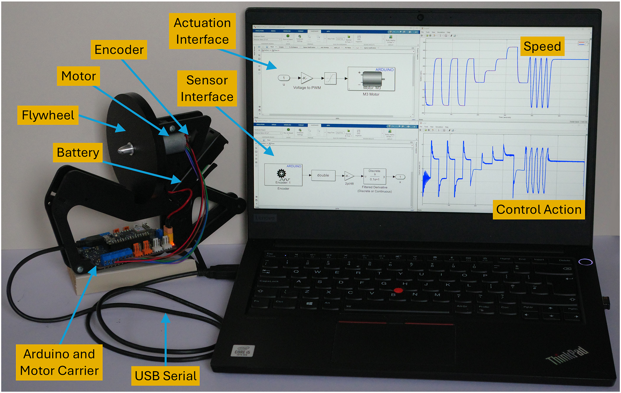
The experimental setup is based on the Arduino Engineering Kit Rev2 ⁴⁷ and includes (i) an Arduino Nano 33 IoT, a 3.3 V microcontroller with a SAMD21 Cortex-M0+ 32bit ARM processor with 256 kB Flash and a maximum clock frequency of 48 MHz; (ii) a 12 V DC motor TRK-370CA-17260-51V-EN which includes (iii) a quadrature hall effect encoder which reads at 48 counts per revolution, and is attached to (iv) a flywheel with a diameter of $0.1$ m and a mass of $0.075$ kg; (v) a support for the motor and flywheel made with components provided with the kit; and (vi) a 4 V Li-ion (Samsung INR 18650-25R) battery which is increased to near 12 V for the motor by using a synchronous boost converter on the Arduino nano motor carrier.

The computer used for programming the microcontroller, data collection and post-processing has an Intel i7 8700k with 16 GB RAM. A USB cable is used to connect the computer to the Arduino board for enabling data transfer, the deployment of the control architecture, and collection of the experimental data. The experimental setup is depicted in Figure 2.

Figure 2.

Experimental setup.

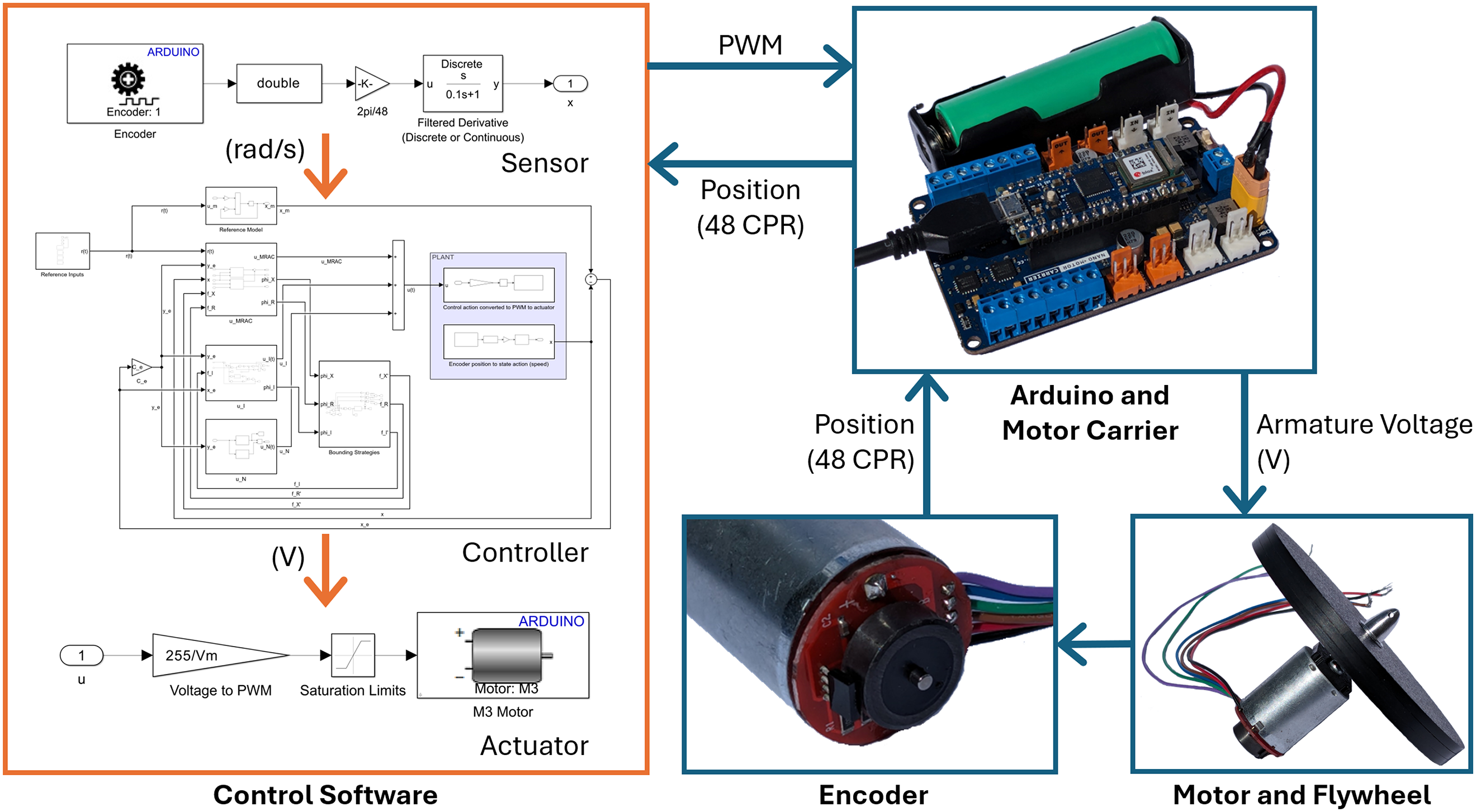
The control architecture, including the control strategies and signal conditioning operations, have been coded in Simulink version 10.6 available in MATLAB R2022b. The schematic of the information flow among the key components and the control software coded in Simulink and running on the microcontroller are depicted in Figure 3. The readings from the encoder are sent to the control software, converted to radians and differentiated with respect to time according to the method recommended by the documentation of the Arduino Engineering Kit Rev 2 ⁴⁸ to obtain the motor/flywheel speed (see also the “Sensor” section in the control software of Figure 3). This speed information is processed together with other signals, such as, the reference speed, by the control algorithm which generates a request of armature voltage to steer the motor speed towards the reference speed. The corresponding pulse width modulation (PWM) signal sent to the power electronics of the motor is represented by a real number in the interval $[-255,255]$ and is obtained from the control action with $\mathrm{PWM}=\mathrm{sat}(255\mathrm{u}/{\mathrm{V}}_{\mathrm{m}})$ (see also the “Actuator” section in Figure 3), where $V_m=12$ V is the maximum voltage across the motor and $\mathrm{sat}$ is the saturation function to limit the PWM variable in the admissible range.

Figure 3.

Schematic of the information flow among the components and the control software.

The “Encoder” block and “M3 Motor” block are provided by the Simulink Support Package for Arduino Hardware add on for MATLAB/Simulink. The MATLAB Support Package for Arduino Hardware is also required to allow the Arduino to connect to MATLAB/Simulink. The Simulink model is deployed to the Arduino by selecting Arduino Nano 33 IoT as the target “Hardware Board”. The code is deployed in the Arduino board by using the ”Monitor and Tune” mode, thus allowing monitoring of the experiment and data acquisition. The Simulink model is compiled with the discrete solver ode2 (i.e., the Heun solver) with a sampling time of $t_s=10$ ms. Experimental data is collected over the USB serial connection and saved in a MATLAB workspace.

Modelling and experimental validation

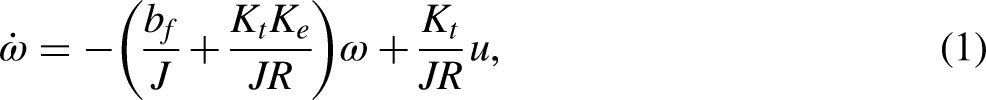
The DC motor speed dynamics can be modelled as a LTI first-order system when the electrical dynamics are much faster than the mechanical dynamics and nonlinearities are neglected. ⁴⁹ Under these assumptions, by denoting $\omega$ (rad/s) as the motor speed (plant state) and $u$ (V) as the armature voltage (control input), the plant model is

$$\dot{\omega }=-(\frac{b_f}{J}+\frac{K_t{K}_e}{JR})\omega +\frac{K_t}{JR}u,$$

(1)

where $J$ (kgm ${}^2$ ) is the moment of inertia of the flywheel and the motor, $b_f$ (Nms) is the coefficient of the linear friction torque acting on the system, $R$ ( $\mathrm{\Omega }$ ) is the armature resistance, $K_e$ (Vs/rad) is the back emf coefficient, and $K_t$ (Nm/A) is the motor torque coefficient.

For the design of control algorithms with fixed control gains (such as model-based proportional integral (PI) and pole placement strategies), estimates of plant parameters are needed. As the moment of inertia of the rotor of the motor can be neglected compared to that of the flywheel, then $J=m{r}^2/2$ , where the flywheel mass $m$ and radius $r$ can be precisely measured, and thus the parameter $J$ can be accurately estimated.

The remaining plant parameters are affected by uncertainties and can be identified through solving a least-square optimisation problem. ⁵⁰ Specifically, by denoting $p=[K_e{K}_t{b}_{f}R]$ as the vector parameter, the optimal set of the parameters $p^{\star }$ is selected as the one that minimizes the following cost function

$$W(p)={\displaystyle {\int }_0^{T_I}({\omega }_E(t)-\hat{\omega }(t;p){)}^{2}dt,\text{with}{p}^l\le p\le p^u,}$$

(2)

where ${\omega }_E(t)$ is the experimental motor speed obtained when the armature voltage is a step function, changing from 11.78 V to -11.78 V with the step occurring at the time instant $t=20$ s; $\hat{\omega }(t;p)$ is the solution of model (1) with plant parameters $p$ and subjected to the same armature voltage step function as the experimental plant; $T_I=40$ s is the duration of the selected identification manoeuvre; and $p^l$ and $p^u$ are vectors that define the lower and upper bounds of each plant parameter, respectively. Moreover, the integral (2) is discretized with the sampling time $t_s$ .

The optimal estimate of the plant parameters $p^{\star }$ has been found numerically using the fmincon function in MATLAB to minimize the $W$ -function in (2), which represents a measure of the mismatch between the experimental results and model predictions. The reader is referred to articles and books dedicated to system identification, for example ⁵⁰ and the references therein, for further details on least-squares methods for plant parameter estimation.

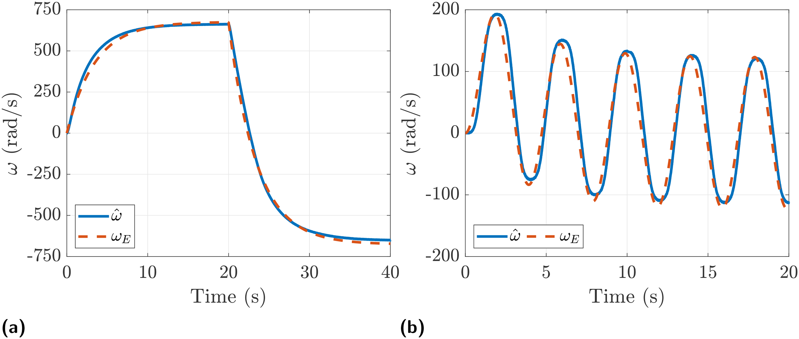
The accuracy of model (1) equipped with the parameter $p^{\star }$ to capture the experimental motor speed when the armature voltage is the step function used for the plant parameter's identification is shown in Figure 4(a). As a validation test, a sinusoidal wave variation of the armature voltage with an amplitude of $11.78$ V and a frequency of $0.25$ Hz is considered. Figure 4(b) shows a good correlation between the experimental results and the model predictions for the selected validation scenario.

Figure 4.

Experimental model validation: ${\omega }_E$ experimental data (red dashed line), and $\hat{\omega }$ model predictions (blue solid line) when the armature voltage is (a) a step function from $11.78$ V to $-11.78$ V and step time $t=20$ s (identification manoeuvre); and (b) a sinusoidal wave with amplitude $11.78$ V and frequency $0.25$ Hz (validation manoeuvre).

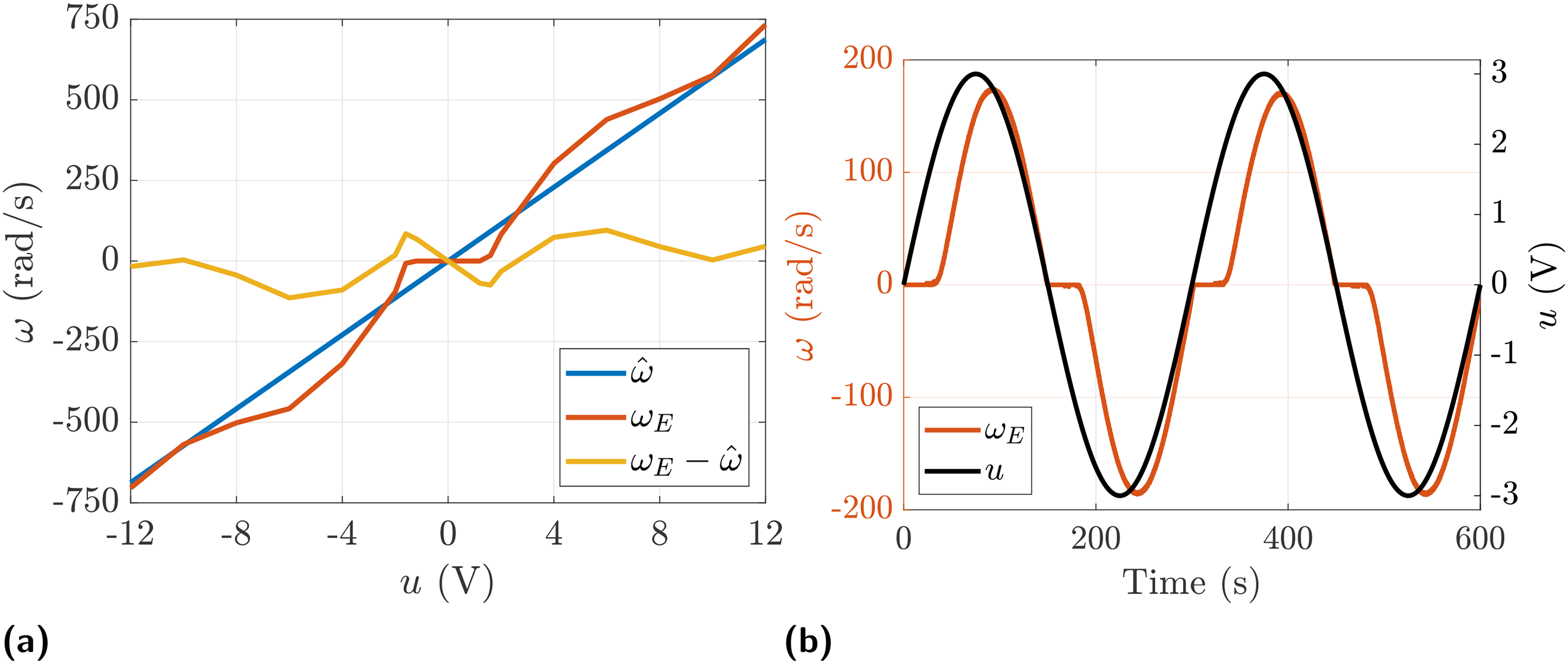
Although the linear model (1) is able to describe the speed dynamics well for the working conditions depicted in Figure 4, further experimental analysis has confirmed the presence of plant nonlinearties which cannot be captured by the DC motor LTI model. Specifically, Figure 5(a) shows that the experimental steady-state speed does not depend linearly with respect to armature voltage. Moreover, (i) the linear approximation provided by model (1) is less precise for inputs around $\pm 5$ V, and (ii) the flywheel does not spin till the magnitude of the input exceeds a threshold of about $2$ V (i.e., there is a dead-zone when $u\in [-2,2]$ ). This dead-zone is due to static nonlinear friction torques not included in model (1). Stiction torques also generate nonlinear stick-slip dynamics, ⁵¹ in other words motions where the flywheel speed suddenly becomes stuck despite smooth variations of the armature voltage. Figure 5(b) shows an example of stick-slip motion experimentally obtained in steady-state conditions when the armature voltage varies as a sinusoidal wave with amplitude $3$ V and period $300$ s. This nonlinear plant behaviour cannot be captured by model (1) as, in accordance with the frequency analysis of LTI systems (as presented in Franklin et al. ⁵² for example), the steady-state output of an LTI system to any sinusoidal input is a sinusoidal wave with the same frequency as the input.

Figure 5.

Experimental plant nonlinearities: (a) variation of the steady-state gain, ${\omega }_E$ experimental speed (red line), $\hat{\omega }$ model predictions (blue line) and corresponding mismatch (yellow line); and (b) stick-slip phenomenon, armature voltage input (gray line) and ${\omega }_E$ experimental speed (red line).

A further system nonlinearity which is not captured by the LTI model (1) is the saturation of the armature voltage. Specifically, the control input $u$ is saturated when its magnitude exceeds $V_m$ (i.e., the actual armature voltage applied to the system is $u_a=\text{sgn}(u)min\{|u|,V_m\}$ ). Saturations in control systems can induce unwanted oscillations of the closed-loop plant response around the required reference and integral windup phenomena when the controller generates control actions exceeding the saturation limits,^53,54 which degrade the tracking performance as also confirmed later with the experimental closed-loop results in the section “Experimental Results”.

The aforementioned nonlinearities are examples of unmodeled nonlinearities and disturbances, which, together with the residual plant parameter mismatches, represent the uncertainties towards which the control system should be robust.

Motivation to MRAC and EMRAC solutions

The target for the tracking control problem is the design of a control strategy to impose to the plant a given reference signal. Consider as a simplifying example a first-order system of the form

$$\dot{x}=ax+bu+\delta ,$$

(3)

where $x$ , $u$ , $\delta \in \mathbb{R}$ are the plant state, control input and disturbance, respectively, while $a$ , $b\in \mathbb{R}$ are the dynamic matrix and input matrix of the plant, respectively. When the plant parameters are known and in absence of disturbances (meaning $\delta =0$ ), a constant reference signal $r\in \mathbb{R}$ can be imposed with preassigned transient dynamics (for example expressed in terms of the settling time of the closed-loop step response) with the following control action

$$u={\varphi }_X^{\star }x+{\varphi }_R^{\star }r,$$

(4)

with ${\varphi }_X^{\star }$ and ${\varphi }_R^{\star }\in \mathbb{R}$ being constant control gains. The feedback gain ${\varphi }_X^{\star }$ can be tuned with the pole-placement strategy to guarantee given transient dynamics while the feedforward gain ${\varphi }_R^{\star }$ is selected to have a closed-loop static gain equal to one, thus having zero steady-state tracking error with respect to the reference signal. ⁵² Specifically, when the control action (4) is substituted into the plant model (3) and $\delta =0$ , then the closed-loop dynamics are

$$\dot{x}=a_{m}x+b_{m}r,$$

(5)

with $a_m=a+b{\varphi }_X^{\star }$ and $b_m=b{\varphi }_R^{\star }$ . The position of the close-loop pole, which determines the closed-loop transient response, is $p=a_m=a+b{\varphi }_X^{\star }$ and can be adjusted to match a desired pole with an ad hoc selection of the control gain ${\varphi }_X^{\star }$ , while the closed-loop static gain can be made equal to one by selecting the feedforward gain as ${\varphi }_R^{\star }=-b^{-1}(a+b{\varphi }_X^{\star })$ . ⁵²

However, plants of engineering interest are often affected by parameter uncertainties and disturbances. By denoting $\mathrm{\Delta }a$ and $\mathrm{\Delta }b$ the uncertainties on the plant parameters $a$ and $b$ , respectively, then actual closed-loop dynamics when the control strategy (4) is applied are

$$\dot{x}=(a_m+\mathrm{\Delta }a+\mathrm{\Delta }b{\varphi }_X^{\star })x+(b_m+\mathrm{\Delta }b{\varphi }_R^{\star })r+\delta .$$

(6)

Because the closed-loop vector field (6) differs from the ideal one due to the presence of the term $(\mathrm{\Delta }a+\mathrm{\Delta }b{\varphi }_X^{\star })x+\mathrm{\Delta }b{\varphi }_R^{\star }r+\delta$ , the actual evolution of the closed-loop system can deviate drastically from the ideal one in (5). However, MRAC solutions can impose desired dynamics of the form (5) despite parameter uncertainties and disturbances by adjusting, or better adapting, the control gains in operation based on the mismatch between the actual plant dynamics and the desired or reference dynamics.

Model reference adaptive control

The control objective of MRAC solutions is to steer the dynamics of the plant toward those of a linear reference system despite parameter mismatches, unmodeled dynamics and disturbances while guaranteeing the boundedness of all closed-loop signals. The reference model dynamics are given by an asymptotically stable LTI system, which, for first-order systems, can be expressed as

$${\dot{x}}_m=a_m{x}_m+b_{m}r,$$

(7)

where $x_m\in \mathbb{R}$ is the state of the reference model, $r\in \mathbb{R}$ is the reference input assumed to be bounded, and $a_m$ and $b_m\in \mathbb{R}$ are the dynamic matrix and the input matrix of the reference system, respectively.

Mathematically, the control target is then to design a control solution such that $x$ converges to $x_m$ asymptomatically (i.e., $x\to x_m$ when the time $t\to +\mathrm{\infty }$ ), for any reference input, initial states of the plant, and reference model (that is, for any $x(t_0)$ and $x_m(t_0)$ , with $t_0$ being time instant when the controller is activated), despite plant parameter uncertainties $\mathrm{\Delta }a$ and $\mathrm{\Delta }b$ and disturbances $\delta$ . MRAC solutions guarantee this control goal by equipping the control strategy with adaptive laws (also known as adaptive rules or mechanics).

The simplest MRAC solution is the following ³

$$u_{\mathrm{MRAC}}(t)=K_X(t)x+K_R(t)r,$$

(8)

where the feedback gain $K_X$ and the feedforward gain $K_R$ change over time according to the following adaptive laws

$$K_X={\varphi }_X,\mathrm{and}{\dot{\varphi }}_X={\alpha }_X{y}_{e}x,$$

(9a)

$$K_R={\varphi }_R,\mathrm{and}{\dot{\varphi }}_R={\alpha }_R{y}_{e}r,$$

(9b)

where ${\alpha }_X$ and ${\alpha }_R\in \mathbb{R}$ are constants known as adaptive weights, and

$$y_e=b_m{x}_e.$$

(10)

with $x_e$ being the tracking error which is defined as the mismatch between the reference state and the plant state, i.e.,

$$x_e=x_m-x.$$

(11)

Remarks:

For MRAC solutions, the reference model is designed based on the control specifications to be imposed onto the closed-loop control system (for example specifications on the transient response or frequency response).

To guarantee that the plant state tracks that of the reference model, MRAC solutions usually require that some matching conditions are met. Specifically, the existence (but not the knowledge) of a control action of the form $u={\hat{\varphi }}_{X}x+{\hat{\varphi }}_{R}r$ , where ${\hat{\varphi }}_X$ and ${\hat{\varphi }}_R$ are constant gains, which is able to transform the plant dynamics into the reference model system (such that $a_m=a+b{\hat{\varphi }}_X$ and $b_m=b{\hat{\varphi }}_R$ ) is required. Matching conditions are always met for plants whose model is expressed in control canonical form (for example first-order systems and electromechanical plant models derived by using the Euler-Lagrange equation). Moreover, for control problems of engineering interest, nominal plant parameters are usually available and can be used to design the reference model such that matching conditions are satisfied. A possible approach is to select as the reference dynamics the nominal plant model controlled through feedback/feedforward control solutions (for example linear quadratic strategies or pole-placement strategies, thus ${\hat{\varphi }}_X={\varphi }_X^{\star }$ and ${\hat{\varphi }}_R={\varphi }_R^{\star }$ in (4)). For first-order systems the ideal gains ${\hat{\varphi }}_X$ and ${\hat{\varphi }}_R$ are

$${\hat{\varphi }}_R=b^{-1}{b}_m\mathrm{and}{\hat{\varphi }}_X=b^{-1}(a_m-a).$$

(12)

The adaptive weights ${\alpha }_X$ and ${\alpha }_R$ must have the same sign as ${\hat{\varphi }}_R$ and represent the rate of variation of the adaptive gains.

The dynamics of the adaptive gains of MRAC solutions (as in (9)) are nonlinear and become states of the control system. Consequently, the analysis of the closed-loop system cannot be carried out via methods used for linear systems (for example utilising the study of the position of eigenvalues ⁵² ) and more sophisticated methods for assessing closed-loop stability and convergence of the error, for example Lyapunov theory and passivity theory, must be used. ³

The classical MRAC solution in (8) can asymptotically impose the dynamics of the reference model to the plant (i.e., $x_e\to 0$ when $t\to +\mathrm{\infty }$ ) in the case of uncertain plant parameters and square-integrable unknown disturbances, that is $\delta \in {\mathcal{L}}_2$ (in other words disturbances for which ${\int }_{t_0}^{+\mathrm{\infty }}\Vert \delta (t){\Vert }^{2}dt$ is finite). On the contrary, EMRAC control solutions can guarantee zero tracking error for a larger class of disturbances, namely bounded disturbances (expressly $\delta \in {\mathcal{L}}_{\mathrm{\infty }}$ , or equivalent disturbances for which there exists a positive constant $\mathcal{G}$ such $\Vert \delta (t)\Vert <\mathcal{G}$ for all $t\ge t_0$ ). This is a key benefit of EMRAC solutions which also opens the way for their applications to plants characterized by non-vanishing disturbances.

Adaptive gains locking strategies

In the case where the plant dynamics are affected by persistent disturbances or unmodeled dynamics (e.g., $\delta =\delta (x,t)$ ) an unbounded drift of adaptive gains may arise when classical adaptive laws, such as those in (9), are utilized to update the adaptive gains, ⁵ as is also shown in the adaptive control literature through the Rohrs’ example.^55,56 Unbounded adaptive gains may not only lead to a degradation of the tracking performance of the reference model but may also lead to closed-loop instability. Mathematically, boundedness of the adaptive gains when adaptive laws as in (9) are used cannot be guaranteed in the presence of persistent disturbances and unmodeled dynamics since the derivative of the Lyapunov function of the closed-loop system is not strictly negative with respect to the adaptive gains.^3,5

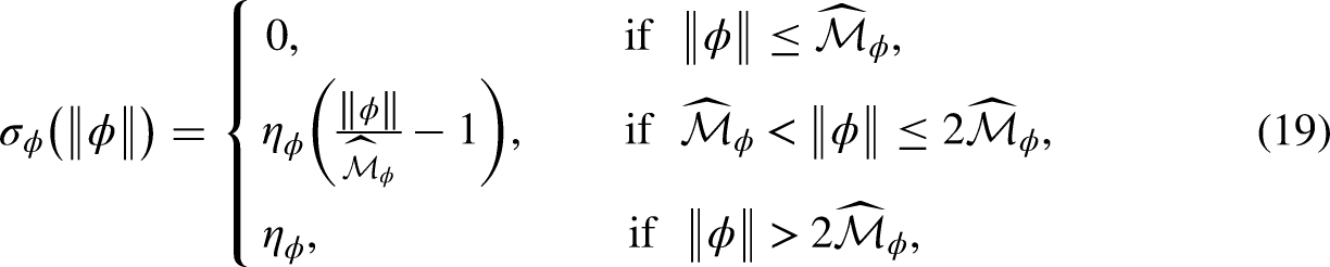
To guarantee bounded adaptive gains despite disturbances and unmodeled dynamics, robust modifications to the classical MRAC adaptive mechanisms are presented in the literature.^3,5 Broadly speaking, these techniques aim to either (i) limit the adaptive gains within a preassigned set; or (ii) equip the adaptive laws with damping mechanisms to prevent the unbounded drift of the adaptive gains. Within this framework, the parameter projection strategy falls under the first category, while the $\sigma$ -modification method is an example of robust modification belonging to the second category. In what follows both of these methods are revised for first order systems. Moreover, both the robust modifications adjust the adaptive laws (9) as

$${\dot{\varphi }}_X={\alpha }_X{y}_{e}x+f_X,$$

(13a)

$${\dot{\varphi }}_R={\alpha }_R{y}_{e}r+f_R,$$

(13b)

where the functions $f_X$ and $f_R$ depend on the strategy adopted to bound the evolution of ${\varphi }_X$ and ${\varphi }_R$ , respectively.

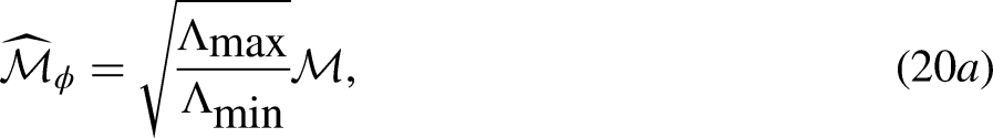
For the design of the robust terms $f_X$ and $f_R$ , the only extra assumption that is required, compared to the classical MRAC algorithm, is that some bounds for the plant parameters are known. This hypothesis is not as restrictive as it might appear at first because the range of variation of the plant parameters are often available for engineering control problems. Specifically, the parameter-projection strategy requires

$${\varphi }_X^l\le {\hat{\varphi }}_X\le {\varphi }_X^u,\mathrm{and}{\varphi }_R^l\le {\hat{\varphi }}_R\le {\varphi }_R^u,$$

(14)

with ${\varphi }_X^l$ , ${\varphi }_R^l$ , ${\varphi }_X^u$ , and ${\varphi }_R^u$ being known bounds for ${\hat{\varphi }}_X$ and ${\hat{\varphi }}_R$ . Furthermore, by defining $\hat{\varphi }=[{\hat{\varphi }}_X{\hat{\varphi }}_R{]}^T$ , the $\sigma$ -modification method requires

$$\Vert \hat{\varphi }\Vert \le \mathcal{M},$$

(15)

with $\mathcal{M}$ being a known positive constant.

Note that, the bounds ${\varphi }_X^l$ , ${\varphi }_R^l$ , ${\varphi }_X^u$ , ${\varphi }_R^u$ and $\mathcal{M}$ can be found based on bounds on the plant parameters, their nominal values, and reference model parameters, for example, as shown in Montanaro and Olm, ²⁴ Montanaro and Olm ⁵⁷ for systems in control canonical forms.

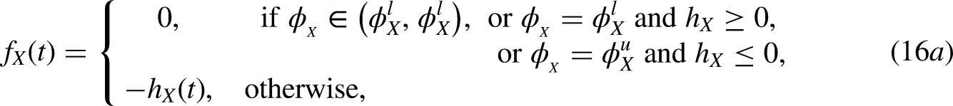
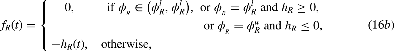
In the case of parameter-projection, the locking functions $f_X$ and $f_R$ in (13) are selected as

$$f_X(t)=\{\begin{array}{cc}0,& \text{if}{\varphi }_{{}_X}\in \left({\varphi }_X^l,{\varphi }_X^l\right),\text{or}{\varphi }_{{}_X}={\varphi }_X^l\text{and}{h}_X\ge 0,\\ & \text{or}{\varphi }_{{}_X}={\varphi }_X^u\text{and}{h}_X\le 0,\\ -h_X(t),& \text{otherwise},\end{array}$$

(16a)

$$\begin{array}{rl}{f}_R(t)& =\{\begin{array}{cc}0,& \text{if}{\varphi }_{{}_R}\in \left({\varphi }_R^l,{\varphi }_R^l\right),\text{or}{\varphi }_{{}_R}={\varphi }_R^l\text{and}{h}_R\ge 0,\\ & \text{or}{\varphi }_{{}_R}={\varphi }_R^u\text{and}{h}_R\le 0,\\ -h_R(t),& \text{otherwise},\end{array}\end{array}$$

(16b)

with $h_X={\alpha }_X{y}_{e}x$ and $h_R={\alpha }_R{y}_{e}r$ .

When the adaptive strategies (13) are coupled with (16), then the dynamics of the adaptive gains ${\varphi }_X$ and ${\varphi }_R$ are constrained in the sets $[{\varphi }_X^l,{\varphi }_X^u]$ and $[{\varphi }_R^l,{\varphi }_R^u]$ , respectively, that is

$${\varphi }_X(t)\in [{\varphi }_X^l,{\varphi }_X^u],\text{and}{\varphi }_R(t)\in [{\varphi }_R^l,{\varphi }_R^u],\text{for all}t\ge 0.$$

(17)

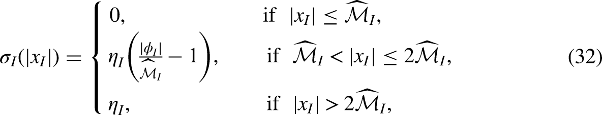
In the case of the $\sigma$ -modification strategy, the adaptive mechanism (13) is completed with

$$f_X=-{\rho }_X{\sigma }_{\varphi }(\Vert \varphi \Vert ){\varphi }_X,\text{and}{f}_R=-{\rho }_R{\sigma }_{\varphi }(\Vert \varphi \Vert ){\varphi }_R,$$

(18)

where ${\rho }_X$ and ${\rho }_R$ are positive constants known as leakage factors, $\varphi \in {\mathbb{R}}^2$ is the stack of the adaptive gains, that is $\varphi =[{\varphi }_X{\varphi }_R{]}^T$ , and the function ${\sigma }_{\varphi }(\Vert \varphi \Vert )$ is defined as

$${\sigma }_{\varphi }\left(\Vert \varphi \Vert \right)=\{\begin{array}{cc}0,& \text{if}\Vert \varphi \Vert \le {\hat{\mathcal{M}}}_{\varphi },\\ {\eta }_{\varphi }\left(\frac{\Vert \varphi \Vert }{{\hat{\mathcal{M}}}_{\varphi }}-1\right),& \text{if}{\hat{\mathcal{M}}}_{\varphi }<\Vert \varphi \Vert \le 2{\hat{\mathcal{M}}}_{\varphi },\\ {\eta }_{\varphi },& \text{if}\Vert \varphi \Vert >2{\hat{\mathcal{M}}}_{\varphi },\end{array}$$

(19)

where ${\eta }_{\varphi }$ is a strictly positive constant and

$${\hat{\mathcal{M}}}_{\varphi }=\sqrt{\frac{{\mathrm{\Lambda }}_{\text{max}}}{{\mathrm{\Lambda }}_{\text{min}}}}\mathcal{M},$$

(20a)

$${\mathrm{\Lambda }}_{\text{min}}=min\{\frac{{\rho }_X}{{\alpha }_X},\frac{{\rho }_R}{{\alpha }_R}\},\text{and}{\mathrm{\Lambda }}_{\text{max}}=\text{max}\{\frac{{\rho }_X}{{\alpha }_X},\frac{{\rho }_R}{{\alpha }_R}\}.$$

(20b)

Qualitatively, when the magnitude of the adaptive gains exceeds the threshold ${\hat{\mathcal{M}}}_{\varphi }$ , negative feedback of the gains are switched on in the adaptive laws (13) which regulate the growth of the adaptive gains and prevent their unbounded drifting.

Enhanced model reference adaptive control

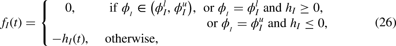
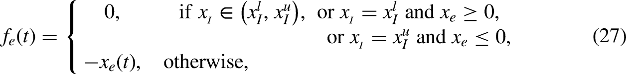
The EMRAC algorithm improves the closed-loop tracking performance of the reference model dynamics by augmenting the MRAC action with an explicit adaptive integral action and an adaptive switching action. When the plant dynamics and reference model are a first-order system, the EMRAC action is

$$u_{\mathrm{EMRAC}}(t)=K_X(t)x+K_R(t)r+K_I(t)x_I+K_N(t)\mathrm{sgn}(y_e),$$

(21)

where $x_I$ is the integral of the tracking error and its dynamics are computed as

$${\dot{x}}_I=x_e+f_e,$$

(22)

with $f_e$ being a term, modelled later, used to prevent a possible unbounded drift of $x_I$ in the case of residual tracking error because of unmatched disturbance and unmodeled plant dynamics.

The EMRAC adaptive mechanisms are

$$K_X={\varphi }_X+{\beta }_X{y}_{e}x,\mathrm{and}{\dot{\varphi }}_X={\alpha }_X{y}_{e}x+f_X,$$

(23a)

$$K_R={\varphi }_R+{\beta }_R{y}_{e}r,\mathrm{and}{\dot{\varphi }}_R={\alpha }_R{y}_{e}r+f_R,$$

(23b)

$$K_I={\varphi }_I+{\beta }_I{y}_e{x}_I,\mathrm{and}{\dot{\varphi }}_I={\alpha }_I{y}_e{x}_I+f_I,$$

(23c)

$$K_N={\varphi }_N,\mathrm{and}{\dot{\varphi }}_N={\alpha }_N{h}_N(|y_e|)-{\sigma }_N(|{\varphi }_N|){\rho }_N{\varphi }_N,$$

(23d)

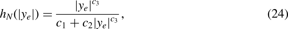
where ${\alpha }_X$ , ${\alpha }_R$ , ${\alpha }_I$ , ${\alpha }_N$ , ${\beta }_X$ , ${\beta }_R$ , ${\beta }_I$ are constants with the same sign of ${\hat{\varphi }}_R$ , ${\rho }_N$ is a strictly positive constant and

$$h_N(|y_e|)=\frac{|y_e{|}^{c_3}}{c_1+c_2|y_e{|}^{c_3}},$$

(24)

with $c_1$ , $c_2$ and $c_3$ being positive constants. The $\sigma$ -modification function ${\sigma }_N(|{\varphi }_N|)$ in (23d) is defined as

$${\sigma }_N(|{\varphi }_N|)=\{\begin{array}{cc}0,& \text{if}|{\varphi }_N|\le {\hat{\mathcal{M}}}_N,\\ {\eta }_N\left(\frac{|{\varphi }_N|}{{\hat{\mathcal{M}}}_N}-1\right),& \text{if}{\hat{\mathcal{M}}}_N<|{\varphi }_N|\le 2{\hat{\mathcal{M}}}_N,\\ {\eta }_N,& \text{if}|{\varphi }_N|>2{\hat{\mathcal{M}}}_N,\end{array}$$

(25)

where ${\eta }_N$ and ${\hat{\mathcal{M}}}_N$ are strictly positive constants.

For EMRAC solutions, the $\sigma$ -modification strategy in (23d) is used to prevent the adaptive gain ${\varphi }_N$ to diverge in the case of unmatched unmodeled dynamics and disturbances. Furthermore, the positiveness of $h_N$ -function (24) limits the use of the parameter-projection method as a gain locking strategy for ${\varphi }_N$ , as it prevents the gain ${\varphi }_N$ from being unlocked once it reaches its admissible upper bound.

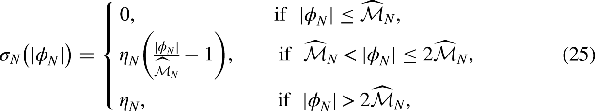
For the adaptive control gains ${\varphi }_X$ , ${\varphi }_R$ and ${\varphi }_I$ in (23), both parameter-projection strategies and $\sigma$ -modification methods can be used. When the EMRAC algorithm is equipped with parameter-projection (PP) strategy it is denoted as EMRAC-PP algorithm. The functions $f_X$ and $f_R$ in (23a) and (23b) are computed as in (16a) and (16b), respectively, while the $f_I$ in (23c) and $f_e$ in (22) are defined as

$$f_I(t)=\{\begin{array}{cc}0,& \text{if}{\varphi }_{{}_I}\in \left({\varphi }_I^l,{\varphi }_I^u\right),\text{or}{\varphi }_{{}_I}={\varphi }_I^l\text{and}{h}_I\ge 0,\\ & \text{or}{\varphi }_{{}_I}={\varphi }_I^u\text{and}{h}_I\le 0,\\ -h_I(t),& \text{otherwise},\end{array}$$

(26)

$$f_e(t)=\{\begin{array}{cc}0,& \text{if}{x}_{{}_I}\in \left(x_I^l,x_I^u\right),\text{or}{x}_{{}_I}=x_I^l\text{and}{x}_e\ge 0,\\ & \text{or}{x}_{{}_I}=x_I^u\text{and}{x}_e\le 0,\\ -x_e(t),& \text{otherwise},\end{array}$$

(27)

where $h_I={\alpha }_I{y}_e{x}_I$ , ${\varphi }_I^l$ and ${\varphi }_I^u$ are the selected lower and upper bound for the gain ${\varphi }_I$ (i.e., ${\varphi }_I(t)\in [{\varphi }_I^l{\varphi }_I^u]$ , for all $t\ge t_0$ ), and $x_I^l$ and $x_I^u$ are the lower and upper bound for the integral of the tracking error (i.e., $x_I(t)\in [x_I^l{x}_I^u]$ , for all $t\ge t_0$ ).

In the case the adaptive mechanism (23) is equipped with $\sigma$ -modification, the resulting strategy is denoted as EMRAC- $\sigma$ and the function $f_X$ , $f_R$ and $f_I$ are defined as

$$\begin{array}{rl}{f}_X& =-{\rho }_X{\sigma }_{\varphi }(\Vert \varphi \Vert ){\varphi }_X,f_R=-{\rho }_R{\sigma }_{\varphi }(\Vert \varphi \Vert ){\varphi }_R,\text{and}\\ f_I& =-{\rho }_I{\sigma }_{\varphi }(\Vert \varphi \Vert ){\varphi }_I,\end{array}$$

(28)

where ${\rho }_X$ , ${\rho }_R$ and ${\rho }_I$ are strictly positive leakage factors, while the $\sigma$ -modification function ${\sigma }_{\varphi }(\Vert \varphi \Vert )$ is that in (19) but with the vector $\varphi$ defined as

$$\varphi ={\left[\begin{array}{ccc}{\varphi }_{{}_X}& {\varphi }_{{}_R}& {\varphi }_I\end{array}\right]}^T,$$

(29)

and the terms ${\mathrm{\Lambda }}_{\text{min}}$ and ${\mathrm{\Lambda }}_{\text{max}}$ used for 20a defined as

$${\mathrm{\Lambda }}_{\text{min}}=min\{\frac{{\rho }_X}{{\alpha }_X},\frac{{\rho }_R}{{\alpha }_R},\frac{{\rho }_I}{{\alpha }_I}\},\text{and}{\mathrm{\Lambda }}_{\text{max}}=\text{max}\{\frac{{\rho }_X}{{\alpha }_X},\frac{{\rho }_R}{{\alpha }_R},\frac{{\rho }_I}{{\alpha }_I}\}.$$

(30)

For the EMRAC- $\sigma$ strategy, the function $f_e$ for limiting the evolution of the integral of the tracking error is designed accordingly as

$$f_e=-{\rho }_I{\sigma }_I(|x_I|)x_I$$

(31)

with ${\rho }_I$ being the corresponding strictly positive leakage factor and

$${\sigma }_I(|x_I|)=\{\begin{array}{cc}0,& \text{if}|x_I|\le {\hat{\mathcal{M}}}_I,\\ {\eta }_I\left(\frac{|{\varphi }_I|}{{\hat{\mathcal{M}}}_I}-1\right),& \text{if}{\hat{\mathcal{M}}}_I<|x_I|\le 2{\hat{\mathcal{M}}}_I,\\ {\eta }_I,& \text{if}|x_I|>2{\hat{\mathcal{M}}}_I,\end{array}$$

(32)

where ${\eta }_I$ and ${\hat{\mathcal{M}}}_I$ are strictly positive constants.

Figure 6 shows the block diagram of the EMRAC algorithm which can be used for representing both the EMRAC-PP and the EMRAC- $\sigma$ strategies. In Figure 6, the adaptive mechanism block updates the feedforward and feedback gains based on the adaptive laws (23).

Figure 6.

Schematic of the EMRAC strategy.

Remarks:

Compared to the MRAC strategy, the EMRAC algorithm is augmented with the adaptive integral control action ( $u_I(t)=K_I(t)x_I$ ) and the adaptive switching control term ( $u_N(t)=K_N(t)\mathrm{sgn}({\mathrm{y}}_{\mathrm{e}})$ ). The adaptive integral control action improves the tracking accuracy of the reference model by compensating for unmodeled biases in the plant dynamics, such as constant disturbances. Moreover, the adaptive switching control action boosts the robustness of the closed-loop tracking performance against rapidly varying bounded disturbances.

The proportional-integral adaptive law used for the gains of the continuous control actions, i.e., $K_X$ , $K_R$ and $K_I$ in (23), improves convergence of the adaptive gains. ⁴ Indeed, the inclusion of the proportional term in the adaptive mechanism allows for quick adjustments of the control gains when there are rapid changes in the tracking error.

The EMRAC approach is more computationally demanding than traditional MRAC algorithms due to the additional adaptive integral and switching control actions. However, implementations of EMRAC solutions on different control units has been investigated (for example dSpace,^23,25 ROS, ³¹ and pixhawk ³³ ) which suggest that the two extra control terms, $u_I$ and $u_N$ , do not compromise the real-time implementability of EMRAC strategies. Moreover, in this paper it is shown that EMRAC solutions can be also implemented in cost-effective microcontrollers, such as Arduino boards.

It has been shown that EMRAC solutions guarantee convergence of the tracking error to zero to square measurable ( ${\mathcal{L}}_2$ ) as well as bounded ( ${\mathcal{L}}_{\mathrm{\infty }}$ ) matched disturbance and unmodeled dynamics. In the case of first order-systems, the asymptotic convergence to zero of the closed-loop tracking error $x_e$ in the presence of bounded disturbances is sketched in the Appendix for the sake of completeness.

The sign function included in EMRAC solutions can induce high-frequency oscillations in the control action which can increase wear of the actuation system. These unwanted oscillations are known in the literature of discontinuous systems as the chattering phenomenon ⁵⁸ and it is a common side effect of control strategies including discontinuous control terms, for example relay control systems with small hysteresis and sliding mode control algorithms. ⁵⁹ In order to avoid the chattering phenomenon, the discontinuous term is commonly smoothed during its implementation, as in Montanaro et al.,^31,32 by adopting

$$\text{sgn}(y_e(t))=\frac{y_e}{|y_e|+ϵ}$$

(33)

with $ϵ$ being a strictly positive constant. Small values of $ϵ$ implies a better approximation of the sign function. Hence, the $ϵ$ -parameter is chosen to be sufficiently large to smooth the control action but without compromising closed-loop tracking performance.

The EMRAC algorithms guarantee that the closed-loop system is globally uniformly ultimately bounded for any bounded external disturbance and unmodeled dynamics (see also ⁵⁸ for the definition of ultimate bounded systems). Practically, this means that the magnitude of the closed-loop state is bounded by a converging function and after a time interval it remains upper-bounded by a strictly positive constant also known as the ultimate bound. Specifically, by defining the closed-loop state as

$${\tilde{x}}_e={\left[\begin{array}{cc}{x}_e& {\varphi }_e\end{array}\right]}^T,$$

(34)

with ${\varphi }_e=\hat{\varphi }-\varphi$ being the mismatch between the adaptive gain vector in (29) and the ideal gain vector $\hat{\varphi }$ defined as

$$\hat{\varphi }={\left[\begin{array}{ccc}{\hat{\varphi }}_{{}_X}& {\hat{\varphi }}_{{}_R}& 0\end{array}\right]}^T.$$

(35)

it is possible to prove that

$$\Vert {\tilde{x}}_e(t)\Vert \le {\gamma }_b(t),\text{for all}t\ge t_0,$$

(36)

with ${\gamma }_b(t)$ defined as

$${\gamma }_b(t)=\{\begin{array}{ccc}\mathrm{\Psi }\left(\Vert \tilde{x}(t_0)\Vert ,t-t_0\right),& \mathrm{if}& t_0\le t\le t_0+\mathcal{T},\\ {\kappa }_{ub},& \mathrm{if}& t>t_0+\mathcal{T},\end{array}$$

(37)

where the time interval $\mathcal{T}$ , after which the tracking error is bounded by the ultimate bound ${\kappa }_{ub}$ , depends on the initial condition $\tilde{x}(t_0)$ ; and $\mathrm{\Psi }:{\mathbb{R}}^{+}\times {\mathbb{R}}^{+}\to {\mathbb{R}}^{+}$ is a $\mathcal{K}\mathcal{L}$ -class function (in other words a function such that for any value $\overline{z}$ , the mapping $\mathrm{\Psi }(r,\overline{z})$ is an increasing function of the variable $r$ and $\mathrm{\Psi }(0,\overline{z})=0$ , while for any $\overline{r}$ , the mapping $\mathrm{\Psi }(\overline{r},z)$ is a decreasing function of $z$ converging to zero when $z\to +\mathrm{\infty }$ ⁵⁸ ).

Controller design

In this paper four adaptive controllers are designed and experimentally compared: (i) EMRAC-PP algorithm, (ii) EMRAC- $\sigma$ algorithm, (iii) the classical MRAC strategy ³ and (iv) the classical MRAC method equipped with the $\sigma$ -modification strategy which is denoted hereafter as MRAC- $\sigma$ . In addition, two control solutions with fixed control gains are designed and used as additional benchmark solutions: (i) a PI controller and (ii) a pole-placement control strategy. ⁵²

The reference model selected for the adaptive solutions is a linear model of the form (7) with time constant $\tau =2.5$ s and unitary static gain (i.e., $a_m=-1/\tau$ and $b_m=-a_m$ ). Considering that the plant time constant is about $3.45$ s, this selection of the reference model reduces the settling time and the rise time of the closed-loop system by approximately $27.5$ % compared to the open-loop plant.

The adaptive weights for the EMRAC-PP and EMRAC- $\sigma$ solutions are the same and have been selected as a trade-off between convergence time and reactivity of the control action. Moreover, the adaptive weights of the proportional part are set ten times smaller than the integral part (that is ${\beta }_i={10}^{-1}{\alpha }_i$ with $i\in \{X,R,I\}$ ). The bounds of the parameter-projection strategy for the EMRAC-PP algorithm, and the thresholds for the EMRAC- $\sigma$ solution have been chosen such that conditions (14) and (15) are satisfied, respectively. Furthermore, the switching action of the EMRAC solutions are computed by using (33) to avoid chattering phenomena of the control action.

The adaptive weights and parameters of the MRAC and MRAC- $\sigma$ algorithms are a subset of those of the EMRAC solutions, and their values have been selected identical to those used for the EMRAC algorithms such that MRAC strategies have the same adaptation rates as the EMRAC solutions.

The plant model used for tuning the pole-placement control gains and PI gains is system (1) where the parameters are those obtained through the procedure detailed in the section “Modelling and Experimental Validation”. Specifically, the fixed control gains of the pole-placement strategy, i.e., ${\varphi }_X^{\star }$ and ${\varphi }_R^{\star }$ in (4), have been tuned as described in the “Motivation to MRAC and EMRAC Solution” section to have the position of the closed-loop pole equal to that of the reference model (i.e., $-1/\tau$ ) and unitary closed-loop static gains. Hence, the closed-loop system controlled via the pole-placement strategy should ideally behave as the reference model selected for the adaptive solutions, thus making the comparison of the closed-loop tracking performance among these control solutions possible.

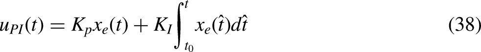
Moreover, for a fair comparison, the reference signal provided to the PI algorithm is the state of the reference model (i.e., the solution of the LTI system (7)), i.e., the control action computed by the PI strategy is

$$u_{PI}(t)=K_p{x}_e(t)+K_I{\int }_{t_0}^t{x}_e(\hat{t})d\hat{t}$$

(38)

where $x_e$ is computed as in (11), while $K_p$ and $K_I$ are the PI control gains. In so doing, the speed behavior that the PI controller will try to impose is that of the reference model. The PI control gains have been tuned based on the plant parameters estimated in the section “Modelling and Experimental Validation” by using the tool “pidtune” in MATLAB.

Experimental results

The closed-loop performance of the controllers designed in the previous section “Controller Design” are experimentally tested on the educational plant presented in the section “Experimental Setup” in different operating conditions. First a long manoeuvre composed of different reference speed profiles with a total duration of $10$ minutes is considered to evaluate closed-loop performance and the corresponding evolution of the closed-loop signals. Then an experimental analysis is presented for different square waves, and the closed-loop tracking performance is quantitatively evaluated via a set of key performance indicators (KPIs) which are usually used in control engineering to compare control solutions. ⁵² Square wave reference inputs have been selected for the second analysis because they are challenging as they generate reference state profiles with steep speed variations which are more difficult to impose.

Long manoeuvre test

The reference input for the long manoeuvre is composed of $4$ sub-manoeuvres denoted as M ${}_i$ , $i=1,\dots ,4$ , where (i) M1 is a square wave with an amplitude of $300$ rad/s, a period of $60$ s, and a duration of $180$ s; (ii) M2 is a sequence of steps at $150$ , $300$ , $450$ rad/s each lasting $40$ s for a total of $120$ s; (iii) M3 is a sinusoidal wave with an amplitude of $400$ rad/s and a period of $20$ s with a duration of $85$ s; and (iv) M4 is a constant at $300$ rad/s with a duration of $135$ s.

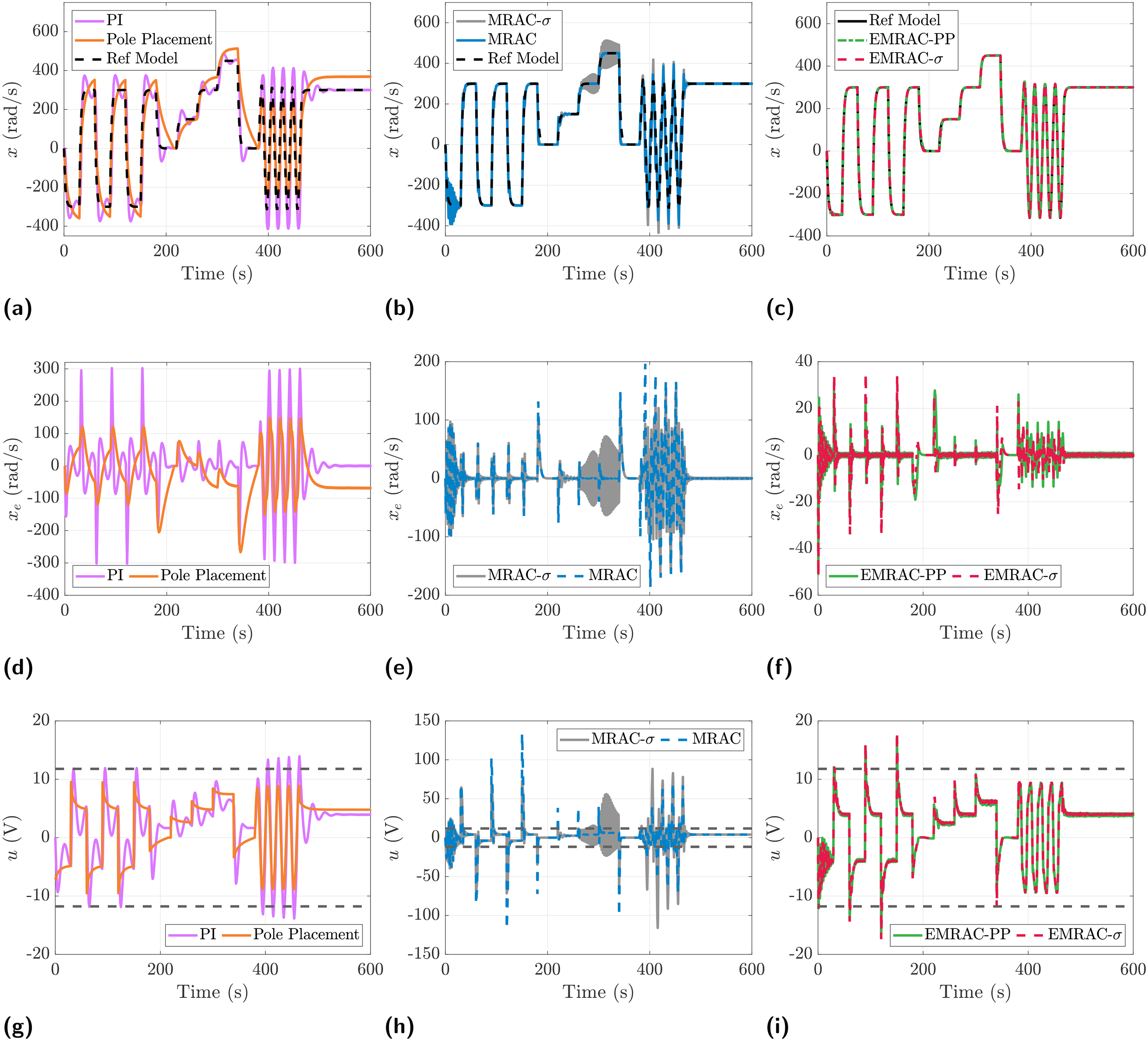
Figure 7 shows the closed-loop performance in terms of speed, error and control action provided by each controller, the evolution of the adaptive gains are shown in Figure 8 for the MRAC solutions, while Figures 9 and 10 depict the dynamics of the adaptive control gains for the EMRAC-PP and EMRAC- $\sigma$ strategies, respectively. Based on the experimental results, the following remarks can be drawn:

Figures 7(a) and 7(d) show that the control strategies with fixed gains do not provide precise tracking of the reference model dynamics mainly because of residual plant parameter uncertainties and nonlinear phenomena discussed in the earlier section “Modelling and Experimental Validation”. Specifically, the pole-placement algorithm does not provide good tracking during the transient nor during the constant steady-state operating conditions. For instance, during the sub-manoeuvre M4, the constant reference is tracked with a steady-state error with a magnitude of about $68$ rad/s (see also Figure 7(d)). This residual error is caused by the residual parameter mismatch between model (1) and the actual plant dynamics. Indeed, Figure 5(a) shows that for steady-state speeds around $300$ rad/s there is significant mismatch between the model predictions and experimental data, and the steady-state armature voltage to keep the speed at $300$ rad/s is experimentally around $3.9$ V. However, with the tuning of the control gains ${\varphi }_X^{\star }$ and ${\varphi }_R^{\star }$ as presented in the section “Motivation to MRAC and EMRAC Solution” and based on the plant parameters estimated in the section “Modelling and Experimental Validation”, the steady-state control action for M4 is about $5$ V which, in agreement with Figure 5(a), gives a steady-state speed of about $368$ rad/s as also observed in Figure 7(a).

As expected the PI strategy provides zero steady-state tracking error for constant reference signals (for example M4). However, plant parameter mismatch and unmodeled dynamics induce overshoots in the step response observed in Figures 7(a) and 7(d) during the tracking of the M2 and M4 signals. Moreover, the closed-loop systems have a bandwidth that does not allow the tracking of the sinusoidal wave M3. As the amplitude of the steady-state sinusoidal speed is larger then the required one, it is deduced that the natural frequency of the experimental closed-loop system is around that of M3.

The MRAC solutions (i.e., the classical MRAC and the MRAC- $\sigma$ strategies) provide better tracking of the reference model dynamics compared to the strategies with fixed gains for most of the long manoeuvre as shown in Figures 7(b) and 7(e). However, for some time intervals (during the first step of the square wave for example) both the MRAC strategy and the MRAC- $\sigma$ algorithm show high frequency oscillations around the reference state with large tracking errors. This unwanted closed-loop behavior is the result of the integral windup phenomenon caused by the saturation of the control action.^52,60,61 Qualitatively speaking, for some operating conditions (for example for rapid variation of the reference input, such as step variations) the MRAC and the MRAC- $\sigma$ strategies are not able to rapidly compensate the mismatch between the reference model and plant speed. The presence of such large errors is then accumulated by the integrals defining the adaptive laws for computing ${\varphi }_X$ and ${\varphi }_R$ , and consequently the adaptive gains increase. Large adaptive gains and errors lead to the generation of control actions above the saturation limits, and thus saturations are activated. During saturation, the adaptive gains are still continuously updated, but these changes do not have an effect on the control action and the plant speed as the actual armature voltage is saturated either at the maximum or minimum value (meaning that there is a loss of control authority). The evolution of the adaptive gains, as seen in Figure 8, during saturation implies that when the system re-enters the linear operating region of the actuator, the actual control gains might be very different from those which would lead to the reduction of the tracking error, thus erroneous control actions can be generated which may increase the mismatch between the reference speed and the actual speed and the process described above repeats, thus leading to a “vicious” cycle of saturations, large errors and demand of large control actions.

Figure 7.

Experimental speed and reference speed (black line), tracking error and control action generated by the controller along with the saturation limits (dark gray dashed lines) for (a, d, g) pole-placement strategy (magenta line) and PI control (orange line); (b, e, h) MRAC (blue line) and MRAC- $\sigma$ (gray line) algorithms; and (c, f, i) EMRAC-PP (green line) and EMRAC- $\sigma$ (red line) strategies.

Figure 8.

Experimental adaptive gains: ${\varphi }_X$ (solid line), ${\varphi }_R$ (dotted line) and magnitude of the adaptive gains $\Vert \varphi \Vert$ for: (a, c) the MRAC algorithm; and (b, d) the MRAC- $\sigma$ strategy.

Figure 9.

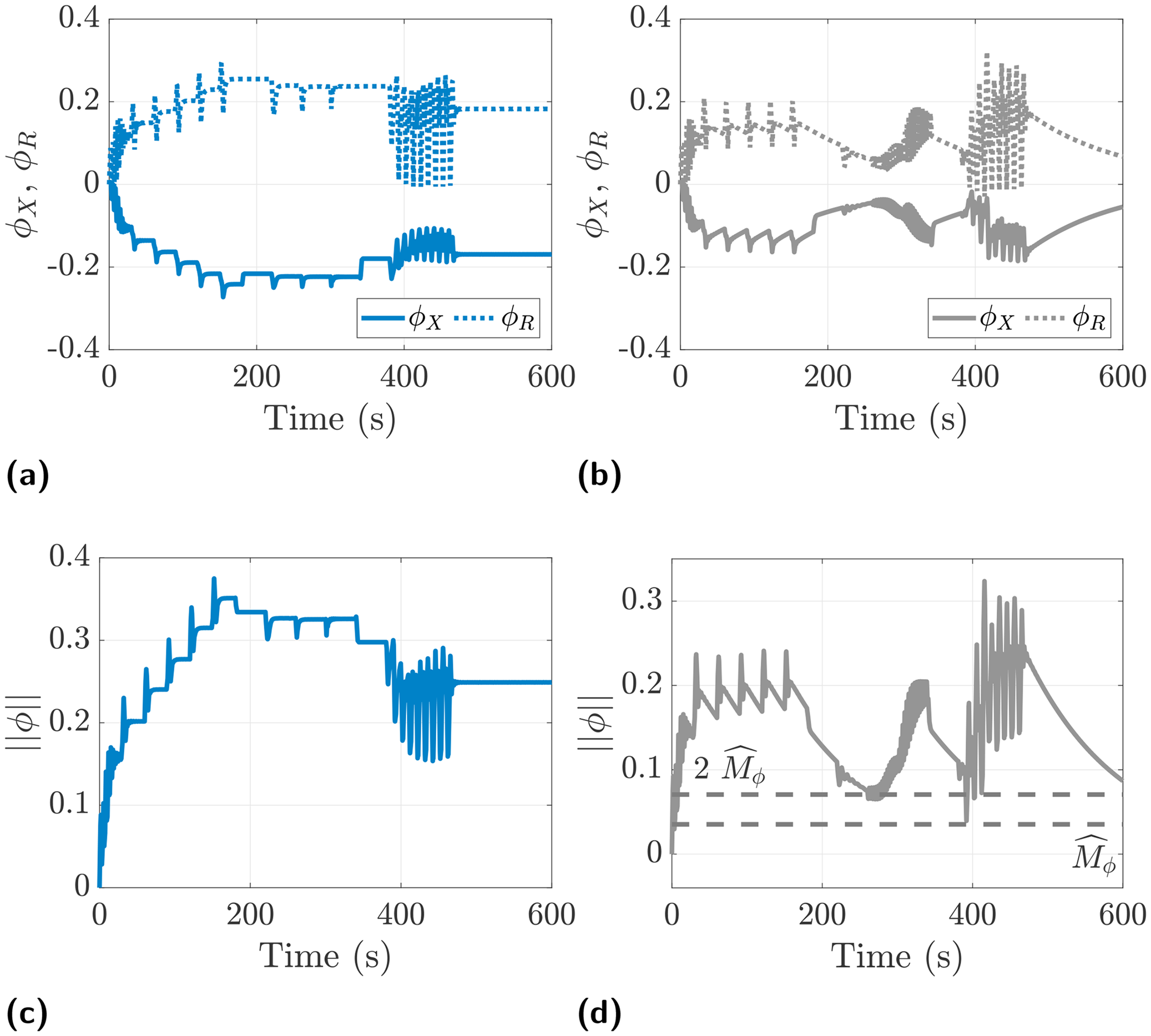
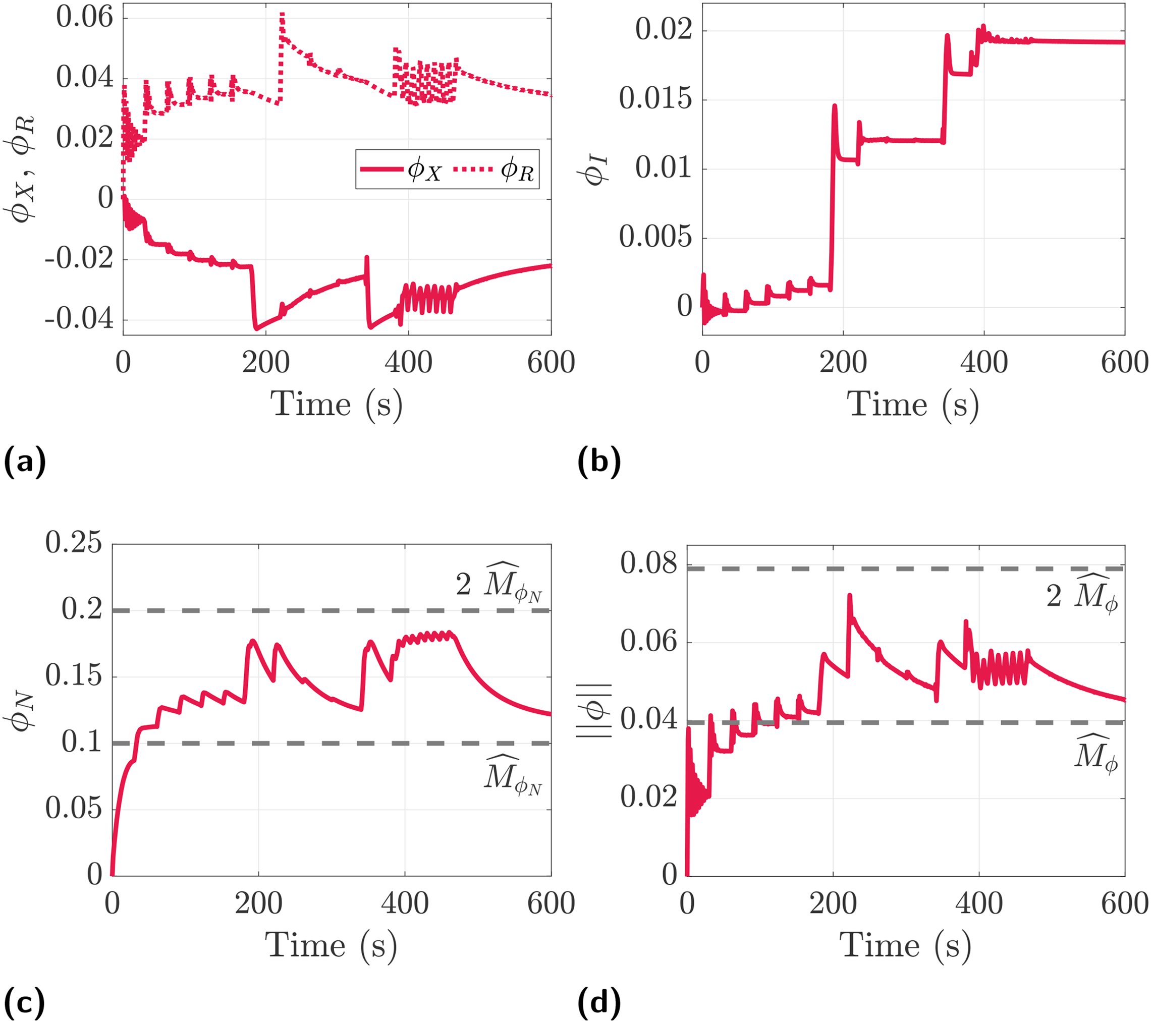
Experimental evolution of the EMRAC-PP adaptive gains: (a) ${\varphi }_X$ , (b) ${\varphi }_R$ , (c) ${\varphi }_I$ , (d) ${\varphi }_N$ and (e) $\Vert \varphi \Vert$ .

Figure 10.

Experimental evolution of the EMRAC- $\sigma$ gains: (a) ${\varphi }_X$ (solid line) and ${\varphi }_R$ (dotted line), (b) ${\varphi }_I$ , (c) ${\varphi }_N$ and (d) $\Vert \varphi \Vert$ .

Figure 7(h) shows the control actions demanded by the MRAC and MRAC- $\sigma$ strategies along with the maximum and minimum applicable armature voltage (dark gray dashed lines). Figure 7(h) confirms the onset of the windup phenomenon, as during the time intervals where the tracking error is large and rapidly oscillates, the control action required by these adaptive solutions is saturated.

It is noted that the windup phenomenon is not limited to adaptive control solutions but can occur also in control strategies with fixed gains including terms based on the integral of the tracking error.^52,60 However, designing anti-windup strategies to include in adaptive laws to avoid unwanted closed-loop behaviours is more complex than for fixed-gain control algorithms, thus, they are beyond the scope of this paper, and the reader is referred to dedicated book chapters^62,63 and recent research articles, e.g., Turner et al., ¹⁶ Turner and Richards, ¹⁷ for studies of MRAC algorithms in the presence of input saturations.

The evolution of the adaptive gains for the MRAC and MRAC- $\sigma$ algorithms along with their magnitude is depicted in Figure 8. Specifically, Figures 8(c) and 8(d) show that the magnitude of the adaptive gains of the MRAC strategy during the square wave M1 is greater than that provided by the MRAC- $\sigma$ solution. The growth reduction of the adaptive gains magnitude given by the MRAC- $\sigma$ strategy is due to the activation of the leakage factor of the $\sigma$ -modification method in (19). Moreover, the leakage factors scheduled by the MRAC- $\sigma$ are constants the majority of the time and equal to ${\rho }_X{\eta }_{\varphi }$ for ${\varphi }_X$ and ${\rho }_R{\eta }_{\varphi }$ for ${\varphi }_R$ , respectively, as the magnitude of the gains, i.e., $\Vert \varphi \Vert$ , is above $2{\hat{\mathcal{M}}}_{\varphi }$ most of the time during the long manoeuvre.

The EMRAC solutions, both the EMRAC-PP and EMRAC- $\sigma$ strategies, provide precise tracking of the reference model dynamics as shown in Figure 7(c). Moreover, Figure 7(f) confirms that the magnitude of the residual speed tracking errors obtained by using the EMRAC strategies are much smaller than the control algorithms with fixed gains and the MRAC methods shown in Figures 7(d) and 7(e), respectively. The EMRAC solutions outperform the fixed gains control methods as they are robust to unmodeled plant dynamics and residual plant parameter mismatches which still remain after the identification method presented in the section “Modelling and Experimental Validation”. Furthermore, the improvement in tracking performance with respect to the MRAC methods is achieved as the EMRAC strategies generate control actions that do not saturate during the long manoeuvre, except for a few spikes that exceed the magnitude $V_m$ but do not jeopardize the tracking of the reference model dynamics. This is confirmed by Figure 7(i), which shows that the control actions demanded by the EMRAC solutions are saturated only four times during M1 and for very short time intervals, when compared to the length of the manoeuvre.

The bounded evolution of the integral part of the adaptive gains for the EMRAC-PP and EMRAC- $\sigma$ strategies are shown in Figures 9 and 10, respectively. The bounded dynamics of these gains along with the boundedness of the tracking error shown in Figures 7(f), imply (i) the boundedness of the magnitude of the adaptive vector $\varphi$ in (29) (see also Figures 9(e) and 10(d)), (ii) the boundedness of the adaptive gains $K_X$ , $K_R$ , $K_I$ and $K_N$ in (23), and thus (iii) the boundedness of the control actions as confirmed in Figure 7(i). For the EMRAC-PP algorithm, Figures 9(a) to 9(c) show the effectiveness of the parameter-projection strategy (16) and (26) to limit the growth of the adaptive gains within their admissible range as well as their locking and unlocking during the long manoeuvre either at the maximum or minimum admissible values, e.g., the gain ${\varphi }_X$ in Figure 9(a) is locked twice at its admissible lower bound ${\varphi }_X^l$ . For the EMRAC- $\sigma$ solution, the magnitude of the gain of discontinuous control action, i.e., ${\varphi }_N$ , and the magnitude of the integral part of adaptive gains of the continuous control actions, i.e., $\Vert \varphi \Vert$ , remain ultimately confined within the $\sigma$ -modification limits, namely ${\hat{\mathcal{M}}}_{{\varphi }_N}\le {\varphi }_N(t)\le 2{\hat{\mathcal{M}}}_{{\varphi }_N}$ and ${\hat{\mathcal{M}}}_{\varphi }\le \Vert \varphi (t)\Vert \le 2{\hat{\mathcal{M}}}_{\varphi }$ , as shown in Figures 10(c) and 10(d), respectively, because the closed-loop tracking errors provided by this control strategy (see also Figure 7(f)) are not large enough to make these adaptive gains exceed the upper limit of the corresponding $\sigma$ -modification strategies.

Square-wave analysis

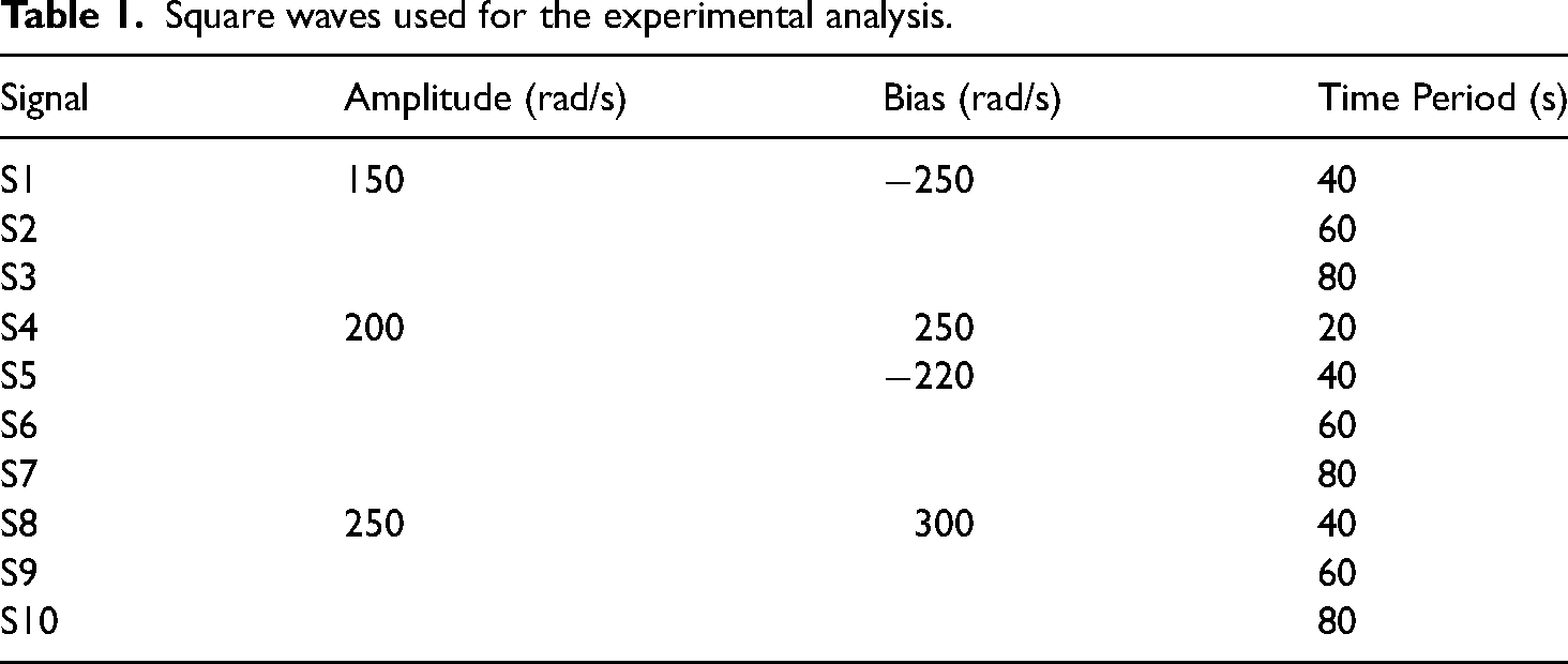
The analysis in the subsection “Long manoeuvre test” has shown that MRAC strategies can induce a high oscillatory behavior of the speed with regards to step variations of the reference signal because of control action saturations, while EMRAC solutions ensure a more precise tracking of the reference model and avoid speed oscillations and control saturations for these more challenging reference inputs. In this context, this section aims to further analyse the closed-loop behavior of the adaptive control strategies under a sudden variation of the reference signal. Therefore, the adaptive control systems have been further tested for ten square waves, $S_i$ , $i=1,\dots ,10$ , for which amplitude, bias and period are detailed in Table 1.

Table 1.

Square waves used for the experimental analysis.

Signal	Amplitude (rad/s)	Bias (rad/s)	Time Period (s)
S1	150	$-250$	40
S2			60
S3			80
S4	200	250	20
S5		$-220$	40
S6			60
S7			80
S8	250	300	40
S9			60
S10			80

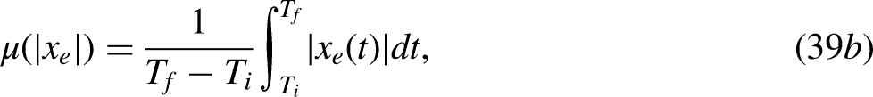
To quantitatively assess the closed-loop behavior a set of KPIs is used. Specifically, the closed-loop tracking performance is evaluated through the following indices

$$\text{RMSE}(|x_e|)=\sqrt{\frac{1}{T_f-T_i}{\int }_{T_i}^{T_f}{(x_e(t))}^{2}dt},$$

(39a)

$$\mu (|x_e|)=\frac{1}{T_f-T_i}{\int }_{T_i}^{T_f}|x_e(t)|dt,$$

(39b)

$$\overline{\sigma }(|x_e|)=\sqrt{\mu \left({[|x_e(t)|-\mu (|x_e|)]}^2\right)},$$

(39c)

$$\kappa (|x_e|)=\underset{T_i\le t\le T_f}{max}|x_e(t)|,$$

(39d)

where RMSE( $|x_e|$ ) is the root mean square error, $\mu (|x_e|)$ and $\overline{\sigma }(|x_e|)$ are the average error and the corresponding standard deviation, respectively, and $\kappa (|x_e|)$ is the maximum error, while $T_i$ and $T_f$ are the initial and final time of the time interval used for computing the KPIs, respectively.

The duration for each square wave in Table 1 is $5$ cycles and the performance indexes have been computed after the transient has been extinguished (therefore over the last four periods).

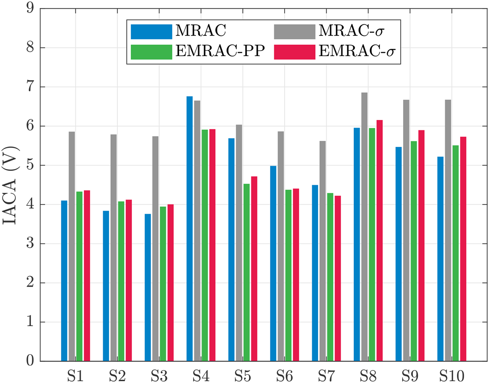
The control action performance is evaluated by computing the integral of the absolute value of the control action normalized with time (IACA) of the actuated control action (i.e., the actual armature voltage which is limited between $\pm V_m$ ). The IACA is a measure of the control effort and is defined as

$$\text{IACA}=\frac{1}{T_f-T_i}{\int }_{T_i}^{T_f}|u_a(t)|dt,$$

(40)

where $u_a=\text{sgn}(u)min\{|u|,V_m\}$ is the actual control action limited within the range $[-V_m,V_m]$ .

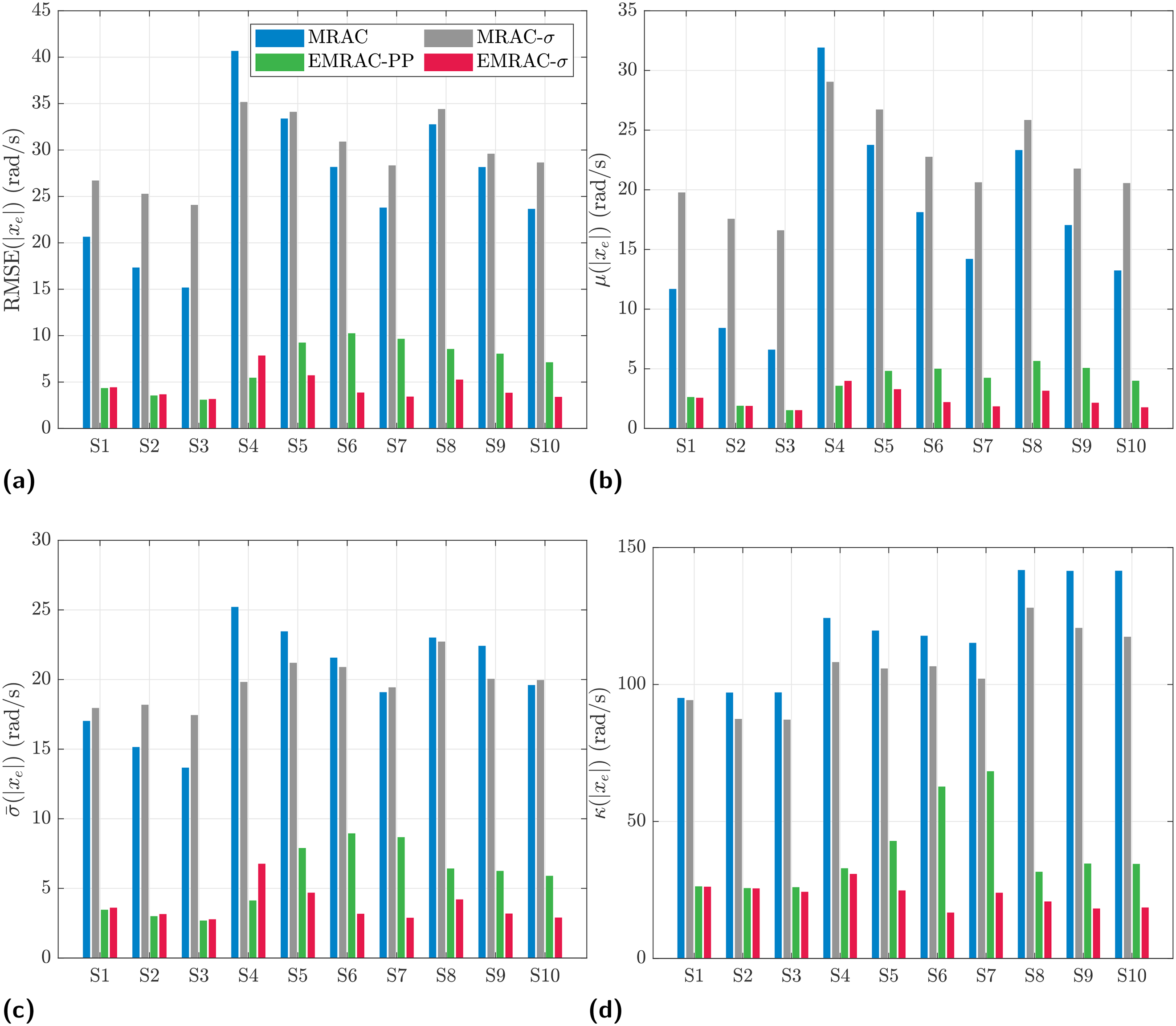
Figures 11 and 12 show the KPIs of the adaptive control solutions for the closed-loop tracking performance and control action, respectively.

Figure 11.

Experimental closed-loop tracking KPIs for the MRAC (blue), MRAC- $\sigma$ (gray), EMRAC-PP (green) and EMRAC- $\sigma$ (red) strategies: (a) RMSE $(|x_e|)$ , (b) average error $\mu (|x_e|)$ , (c) standard deviation $\overline{\sigma }(|x_e|)$ and (d) maximum error $\kappa (|x_e|)$ .

Figure 12.

Experimental IACA for the MRAC (blue), MRAC- $\sigma$ (gray), EMRAC-PP (green) and EMRAC- $\sigma$ (red) strategies.

Based on Figures 11 and 12, the following remarks are made.

The EMRAC solutions provide an RMSE smaller than the MRAC strategies. Figure 11(a) shows that the EMRAC-PP solutions reduces the RMSE index (i) by $2.75$ to $7.4$ times compared to the MRAC algorithm, and (ii) by $3$ to $7.8$ times compared to the MRAC- $\sigma$ algorithm. The reduction factor improves when the MRAC approaches are compared to the EMRAC- $\sigma$ solution. Indeed, the reduction factors for the RMSE provided by the EMRAC- $\sigma$ strategy are in the range $[4.7,7.3]$ and $[4.5,8.4]$ times when compared to the MRAC and MRAC- $\sigma$ solutions, respectively. Moreover, the RMSE for the EMRAC-PP is always below $10$ rad/s, while, except for S4, the EMRAC- $\sigma$ provides an RMSE always either at or below about $5$ rad/s.

Figures 11(b) and 11(c) show that for all the square waves the EMRAC strategies not only substantially reduce the average error $\mu (|x_e|)$ compared to the MRAC algorithms, but also the spread of the speed error around the corresponding average decreases as the standard deviation is reduced. For instance, the EMRAC-PP solution reduces the $\mu (|x_e|)$ -index by at least $3.3$ and $4.3$ times with respect to the MRAC and MRAC- $\sigma$ methods, respectively. In the case of the EMRAC-PP, the spread of the error around the average is reduced by a factor that ranges from $3$ to $6.1$ when compared to the MRAC algorithm, and from $2.24$ to $6.5$ when compared to the MRAC- $\sigma$ strategy. The standard deviation is further reduced when the EMRAC- $\sigma$ algorithm is used. Specifically, for the EMRAC- $\sigma$ , the reduction factor varies in the range $[3.72,7]$ compared to the MRAC, and $[3,7]$ compared to the MRAC- $\sigma$ algorithms, respectively.

Maximum errors are also reduced when comparing the EMRAC solutions to the MRAC strategies as confirmed in Figure 11(d). Specifically, the EMRAC-PP reduces the maximum error with a factor that are in the range $[1.7,4.5]$ times when compared to the MRAC algorithm, and $[1.5,4]$ when compared to the MRAC- $\sigma$ strategy, respectively. The attenuation factor provided by the EMRAC- $\sigma$ for the $\kappa (|x_e|)$ -index is larger and varies in the range $[3.6,7.8]$ times when compared to those provided by the MRAC algorithm, and $[3.4,6.6]$ times when compared to those obtained by the MRAC- $\sigma$ method, respectively.

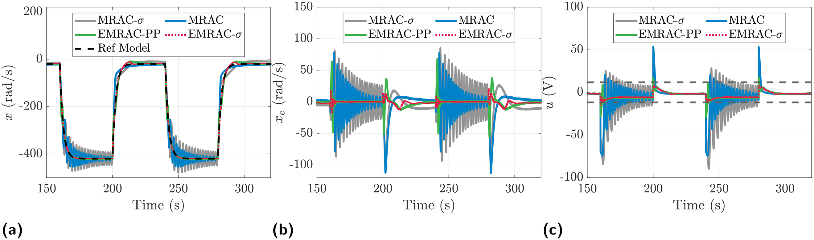
The analysis of the IACA-index in Figure 12 shows that the control effort required by the EMRAC solutions is comparable to that required by the MRAC strategy and either similar or smaller when compared to that demanded by the MRAC- $\sigma$ algorithm. Hence, the EMRAC strategies can improve closed-loop tracking performance without an increase in the control effort. As shown in subsection “Long manoeuvre test”, the tracking performance improvements are achieved as the EMRAC strategies better adjust the control action to quickly track the reference model state despite unmodeled dynamics and disturbances. On the other hand, the larger tracking errors obtained via the MRAC methods generate larger adaptive gains and control actions, which ultimately are saturated. These control action saturations then result in larger tracking error oscillations, preventing the actuator from operating in the linear region. The loss of closed-loop tracking performance due to activation of saturations is also confirmed by a further analysis of the control actions which shows that, for the reference signals in Table 1, the control action generated by the MRAC and MRAC- $\sigma$ algorithms is saturated on average about $20.5$ % and $36$ % of the duration of each square wave manoeuvre, respectively. The average percentage duration of the control action saturation for the square waves in Table 1 reduces to $2.3$ % and $1.44$ % for the EMRAC-PP and EMRAC- $\sigma$ solutions, respectively. Figure 13 shows the tracking performance and the control action provided by each adaptive controller for the S7 reference signal. In this case, the percentage time the control signal in Figure 13(c) is saturated is (i) $15.84$ % for the MRAC, (ii) $30.78$ % for the MRAC- $\sigma$ , (iii) $2.26$ % for the EMRAC-PP, and (iv) $0.39$ % for the EMRAC- $\sigma$ . Consequently, it is expected that the EMRAC- $\sigma$ strategy provides the best closed-loop tracking performance while the worst is given by the MRAC- $\sigma$ algorithm. This is confirmed by Figures 13(a) and 13(b) and Figure 11. Figure 13 also shows that the tracking performance given by the MRAC and MRAC- $\sigma$ significantly improves when their corresponding demanded control actions are within the admissible bounds for the motor armature voltage.

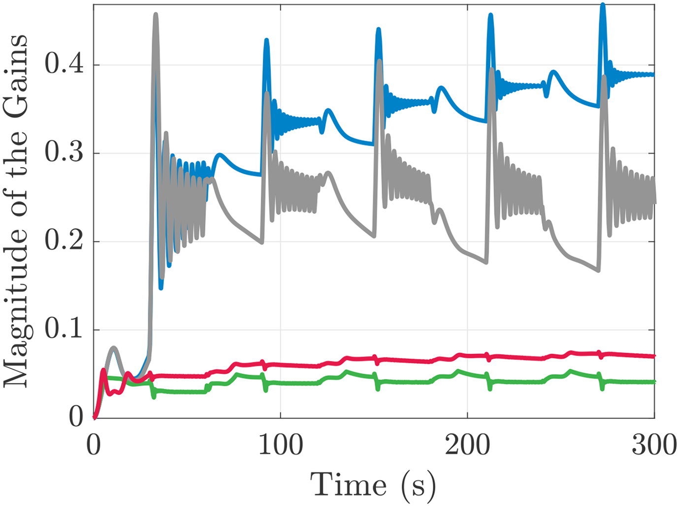
An example of the evolution of the magnitude of the adaptive gains of continuous control actions is depicted in Figure 14 for the reference signal S9 in Table 1. This figure shows a drift in the gains of the MRAC algorithm due to unmodeled dynamics, which can also ultimately induce closed-loop instability. On the contrary, the parameter-projection and $\sigma$ -modification strategies, included in the MRAC- $\sigma$ , EMRAC-PP and EMRAC- $\sigma$ , are effective to keep the evolution of the adaptive gain vector $\varphi$ bounded.

Figure 13.

Experimental results for the S7 reference signal for the MRAC (blue line), MRAC- $\sigma$ (gray line), EMRAC-PP (green line) and EMRAC- $\sigma$ (red line) strategies: (a) speed and reference speed (dashed black line), (b) tracking error, and (c) control action generated by the controller along with the saturation limits (dark gray dashed lines).

Figure 14.

Experimental magnitude of the control gain vector $\varphi$ for the S9 signal in table 1 for the MRAC (blue), MRAC- $\sigma$ (gray), EMRAC-PP (green) and EMRAC- $\sigma$ (red) strategies.

Conclusion

This paper has revised the EMRAC strategy, its design, and aspects of the closed-loop dynamics through the use of a first-order experimental educational plant, thus facilitating the learning of the EMRAC strategy for students who may not be familiar with adaptive control and MRAC solutions. The EMRAC tracking performance has been experimentally compared with that of linear controllers commonly taught in undergraduate control engineering modules and classical MRAC solutions, and it has been shown that EMRAC algorithms outperform these baseline control strategies. Specifically, experimental data has shown that EMRAC methods can be used as an effective approach to impose the ideal closed-loop dynamics provided by a pole-placement strategy, despite plant parameter mismatches which reduce the tracking capability of the classical linear solution with fixed gains. Moreover, compared to the baseline MRAC techniques, the EMRAC solutions are better able to keep the plant within the linear operating region, thus avoiding control input saturation, which, together with the additional adaptive EMRAC terms, improves the tracking of the reference model dynamics. Future research work on the EMRAC algorithm will include extensions to further increase its robustness to unmodelled nonlinear dynamics, e.g. by means of neural network / artificial intelligence methods.