
Abstract
In this work, we adopt a problem-based learning approach to develop an integrative bachelor project that relies on competences acquired from basic courses in mathematics, mechanics and computation. In this sense, the proposed project tries to pave the way from “apparently disconnected” concepts gained through previous studies toward the field of computational mechanics. On this basis, we study the motion of a particle along an arbitrary curve in space subject only to the gravitational field, the so-called sliding bead. Although this is a classic problem in mechanics, it has a substantial richness from a theoretical and practical point of view where the student reinforcing abstract skills and exploring different aspects of its numerical solution are allowed. Along this path, we start with the modeling process. This is followed by a stability analysis of the governing differential equations. Later on, we present a moderate introduction to classical numerical time integration by considering several numerical schemes and the well-known Matlab add-on Simulink. Finally, we present a brief discussion about how the proposed project allows articulating concepts of mathematics, mechanics, and computation in engineering programs of studies at horizontal and vertical levels.
Introduction
Physics and mathematics are the backbones of practically all courses of studies in engineering. Despite the different programs around the world, bachelor’s plus master’s or five-year integrated programs, all of them contain several courses on mathematics and physics in their first years. Thus, such courses should be regarded as very important appetizers for the later skill development.
The fragmentation of content and the lack of articulation between physics and mathematics can hinder the learning of new concepts as well as their subsequent utilization; the reason why there exist several proposals to articulate the concepts conveyed among different courses.1–4 Describing the motion of a particle or a material body (kinematics) may be a challenge for students taking their first steps, specially toward building engineering thinking. On this basis, the work reported by Cashman and O’Mahony 5 empathizes the need for a teaching process that allows the use of different approaches to achieve a more integral learning framework. Those authors suggest to link laboratory observations with real-world concepts, to use multimedia platforms and active and peer learning.
Many of the courses of a typical engineering program follow a classical approach, i.e., theoretical lectures, practical lectures, and, in the best of the cases, lab works. All these stages are contained in several small work packages or units that have to be addressed during the whole semester. A typical problem experienced by teachers with this form of teaching is that most of the time the units are quite independent from each other and the exercises to solve are extremely simple and/or not related to real-life problems or at least concrete applications. One possible path to circumvent this shortcoming is to adopt the teaching paradigm denominated problem-based learning (PBL).
PBL is a modern teaching paradigm with focus on the solution of a concrete complex problem, which is used not as a final target, but as a mean to incorporate knowledge and competences from more abstract disciplines. At the core of this methodology, the problem into consideration is broken down into small problems that are sequentially solved, ranging from the analysis to the design and gradual development of its solution. Although this paradigm was developed during the 1970s in medicine, it has also been effectively applied to other programs such as economics, law, and engineering. 6 Especially in engineering this paradigm fits quite well, but its applicability in fields such as applied and pure mathematics is still undergoing research. 7 Promisingly, PBL allows for an effective implementation of sustainable development in university environments, 8 for education of sustainability and sustainable education 9 and also for joint learning methods. 10 Along with this contribution, we consider the systematic application of PBL within the engineering educational context.
According to our own experience, carrying out first experiences with this paradigm can be challenging due to (a) a teaching staff exposed mostly to classical approaches; (b) reduced availability of material on its practical implementation for science, technology, engineering, and mathematics disciplines; (c) limited availability of professional support for teachers at institutional level; and, (d) the difficulties associated with the implementation of this paradigm in courses with an official program relying on a classical approach. Despite these challenges, our teaching experience indicates that two key results are the engagement of the students that result in students more actively interested in concrete engineering topics, and the number of creative solutions that can arise, that usually are not foreseen. The success of this approach can, in turn, result in the development of new integrative problems, involving ongoing research, with which teachers are working while developing teaching activities. This attempt to bridge research and teaching is proven to be successful, so we strongly suggest to implement it whenever possible.
Nevertheless, a characteristic challenge with the PBL is to remind the students to develop a general perspective on their project solution. For a comprehensive description of the challenges associated with PBL the reader is referred to the work of Boud and Feletti. 11 Sometimes they are very focused on the background and knowledge related to the problem they chose to solve, so they tend to leave aside the course contents that are not directly related to it. In those cases, it is necessary to emphasize that similar solutions to their particular problem can be applied to a broader range of situations. This is essential to develop critical thinking. 12 It is also important to guide them into alternating roles and tasks within their project to gather all the necessary abilities planned for the semester. Finally, the evaluation of the individual contribution of each student to the outcome of the project is challenging.
In this contribution, we propose to apply PBL not at the level of a single course, but at a broader level within a bachelor program. The idea is to offer an integrative bachelor project that relies on the competences, i.e., knowledge or skills, acquired from several basic curses in mathematics, mechanics, and computation. Thus, the target students are expected to be at a senior bachelor level. For this purpose, we propose a project that deals with the dynamic behavior of a sliding bead along a predefined trajectory. Our approach substantially differs from the one proposed by Hennessey and Kumar, 13 because we encourage the students to develop all their own software components without resorting to commercial packages. The showcase starts with the modeling, i.e., the analysis of the system and its description by means of a set of governing equations for the associated initial-value problem. Once the set of governing equations is at hand, we proceed with the investigation of its stability. Upon identification of the system’s critical points, we follow two complementary approaches: the first one relies on the linearization of the equations of motion and eigenvalue analysis; and, the second one relies on some energetic analysis. Once the stability has been elucidated to a good extent, we move on with the numerical solution of the governing equations. Finally, we carry out classical numerical integration in time by considering several numerical schemes. Alternatively, we also perform the integration of the governing equations by means of Simulink. In addition and to provide means for a better understanding of the subject, we also employ techniques for visualization that allow us to reinforce the fixation of concepts, as reported by Pena et al. 14 in the context of mechanical vibrations.
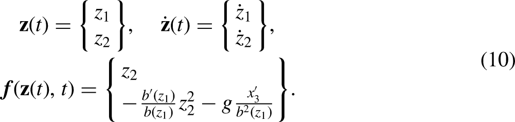
Problem-based learning
In this section, we describe the main components of a PBL integrative project proposed, at first glance, within the scope of computational mechanics. According to Oden et al., 15 computational mechanics can be regarded as a sub-discipline of theoretical and applied mechanics concerned with the use of computational methods and devices to study events governed by the principles of mechanics. However, computational mechanics can be seen as well as a sub-discipline of predictive computational science. This branch of computational science deals with the formulation, calibration, numerical solution, verification, and validation of mathematical models targeting at predicting the behavior of mechanical systems. Moreover, this can also be associated with the presence of uncertainties, see for instance Oden et al. 16 Nevertheless and for the sake of simplicity, we focus, along this work, on mechanical systems that are not affected by uncertainty in any way, shape, or form.
At any rate, this field is by no means a stand-alone field and builds upon a good number of several areas such as: (a) mathematics; (b) mechanics; and, (c) computation. Next, we indicate the branches of the areas previously mentioned that are necessary to carry out the project proposed and are taught as basic blocks within any modern course of studies in engineering. We provide brief descriptions presented in a language format accessible to the target group of students and teachers. Figure 1 presents a schematic time-line for a proposed PBL project on computational mechanics. It is intended to be framed in the last semester of a typical bachelor’s degree in engineering, physics, mathematics, or similar programs. The main goal of this project is twofold: To reinforce the previous knowledge and developed skills or even include partially new knowledge or develop new skills while solving the integrative project, and to introduce the student into the exiting field of computational mechanics.
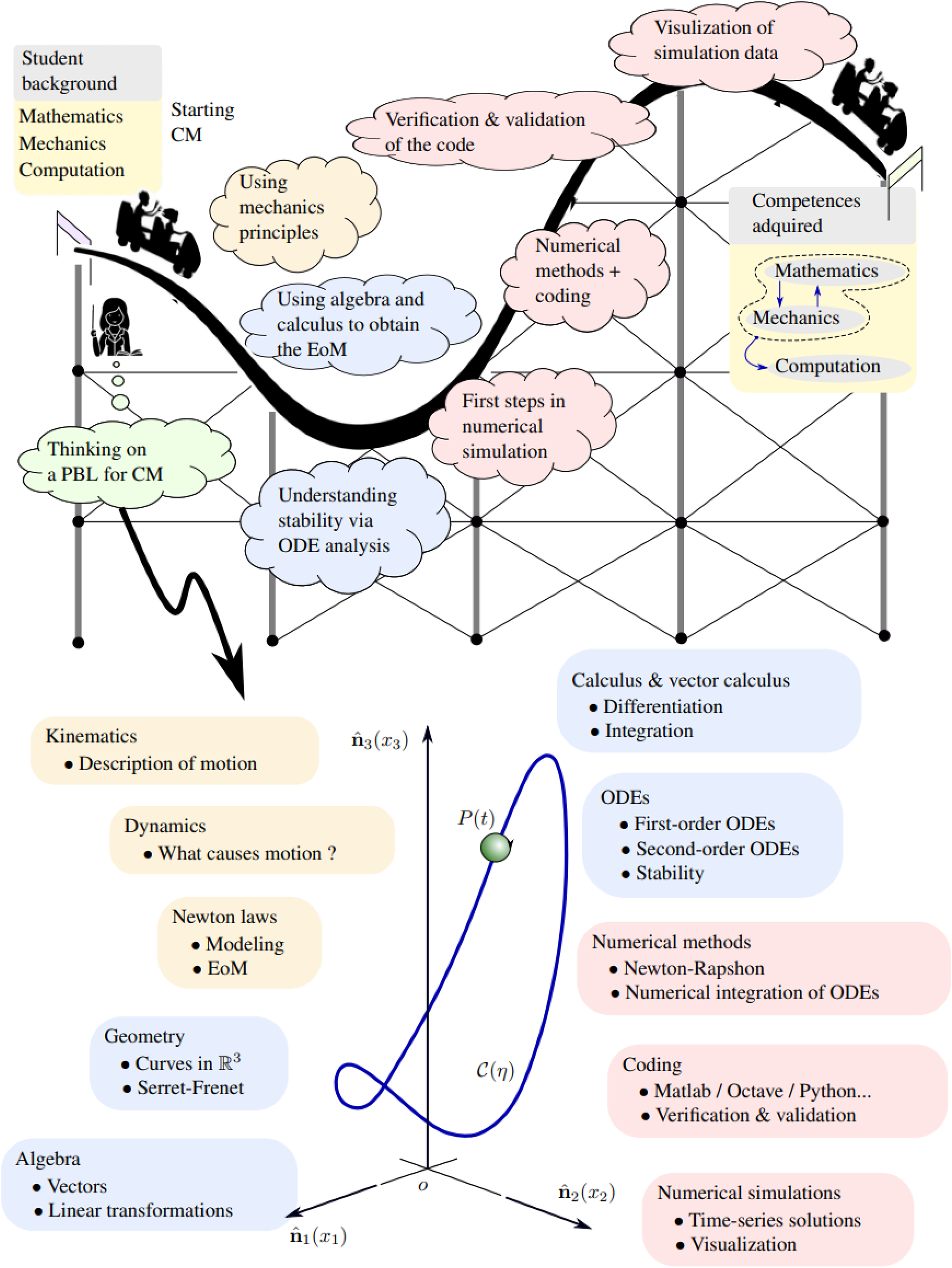
(Top) Timeline of the proposed integration course on computational mechanics, (Bottom) SBP, PBL proposed as the core of the integrative project on CM. CM: computational mechanics; SBP: sliding bead problem; PBL: problem-based learning.
Mathematics
Algebra deals with sets and operations defined on these sets satisfying certain rules. For instance, a vector space is a set of elements denominated vectors. Moreover, such vectors can be added together and multiplied by a scalar, satisfying the rules called vector axioms. Calculus studies the computation of derivatives and integrals of real functions. Whereas the derivation process allows to determine the instantaneous rate of change of a given function, the integration process allows to determine the area below the curve described by a function. Geometry investigates the local properties of certain objects. For instance, when we consider a non-straight three-dimensional curve, the way in which it bends can be described by its curvature meanwhile the way in which it twists can be described by its torsion. Vector calculus deals with the computation of derivatives and integrals of vector fields. Exemplary, the work done by a vector field along a curve is given by the line integral over the vector field. Ordinary differential equations(ODEs) considers the analysis and solution of differential equations depending on a single independent variable. For instance, the phase portrait represents geometrically the behavior of a system governed by a set of ODEs. Moreover, this representation is a powerful tool to understand the system’s stability.
Mechanics
Kinematics studies the description of motion of a material body or a collection of material bodies without considering how such is originated or sustained. For instance, the trajectory of a particle is represented as a vector function of time. Moreover, the velocity is the temporal rate of change of the trajectory while the acceleration is the temporal rate of change of the velocity. Kinetics investigates how forces and torques give origin or sustain the motion of a material body or a collection of material bodies. Exemplary, in a roller coaster, the train is pulled uphill by a chain that counteracts the train’s weight while downhill this is accelerated by the only presence of gravity. Newtonian mechanics deals with the systematic application of Newton’s laws of motion to derive the governing equations of a material body or a collection of material bodies. In particular, the second law states mathematically that the change of momentum of the material body with respect to an inertial frame, a frame that is at rest or moves at constant velocity, is equal to the acting forces. Should the mass be invariant, then the momentum is equal to mass times acceleration. Lagrangian mechanics deals with the systematic application of the principle of least action to derive the governing equations of a material body or a collection of material bodies. In such a context, the Lagrangian function is defined as the kinetic energy minus the potential energy, where the first one is the part of the energy purely associated with the motion, and the second one is the part of the energy purely associated to force fields whose work only depends on the final and original configurations (positions). The action integral is then defined as the integral of the Lagrangian function over a finite, but arbitrary time interval. Upon its variation, a “small” change at fixed time, followed by some algebraic manipulations, the governing equations, the so-called Euler-Lagrange equations, arise. Constrained systems studies the motion of a material body or a collection of material bodies subject to certain restrictions depending on their position and velocity. For example, in a roller coaster, the train is constrained to follow the path defined by the rails.
Computation
Numerical analysis deals with the development and understanding of algorithms intended to approximately solve mathematical problems through their implementation and execution on digital computers. Exemplary, is the computation of trajectories of a particle under the action of external force fields, which are governed by an ODE. Programming considers the design and implementation of a set of instructions targeting at the automation of a given task. This is materialized in form of an executable program that runs on digital computers. For instance, we can write a computer code for the computation of trajectories of a particle under the action of external force fields. Simulation deals with the execution of computer programs that implement mathematical models to study physical systems. Such computational models are used then to carry out predictions on the system’s behavior. In particular, we can carry out simulations to predict how the free trajectories of a particle will look like when starting from a specific position and velocity. Visualization considers the representation of abstract data, e.g., coming from simulation, in a visual form that facilitates their analysis and interpretation. Moreover, visualizations can be static, such as the time history of the position and velocity of a particle, or dynamic, such as an animated video showing how a particle moves along a trajectory. Human–machine interaction studies the design and utilization of computer technology, hardware or software, paying special attention on how users and computers interact. Whereas the monitor, keyboard and mouse are hardware elements enabling for human-machine interaction, the graphical user interface of a computer program is a software element.
The success of this integrative project depends to some extent on the conceptual richness and versatility of the PBL in order to exploit acquired competences, to pose new questions, explore different solution procedures, combine knowledge coming from different branches (mechanics, mathematics and computation), and challenge students to acquire new skills and providing a natural framework for reinforcing knowledge. On this basis, we propose to study the motion of a particle along an arbitrary curve in space, the so-called sliding bead problem (SBP). Although this is a classic problem in mechanics, the SBP is rich enough from a theoretical point of view to allow the student to reinforce abstract skills. At the same time, this problem allows exploring different aspects of its numerical solution, giving the student an integrated vision of theory and numerical simulation. Figure 1 shows a schematic of the SBP along with the main topics to address.
Along the remaining of this contribution, we are also going to point out where specific knowledge or skills are required for a successful accomplishment of the integrative project proposed.
Sliding bead modeling
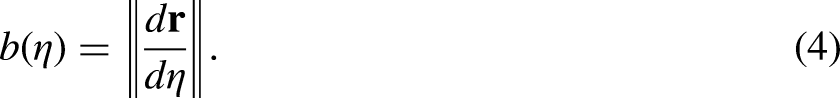
In this section, we present the modeling process for the SBP introduced above. To such an end, let us consider a particle
For a given dynamic system, the number of DoFs is an invariant property. For the sake of clarity, we assume: (a) a global (or Newtonian) orthonormal reference frame
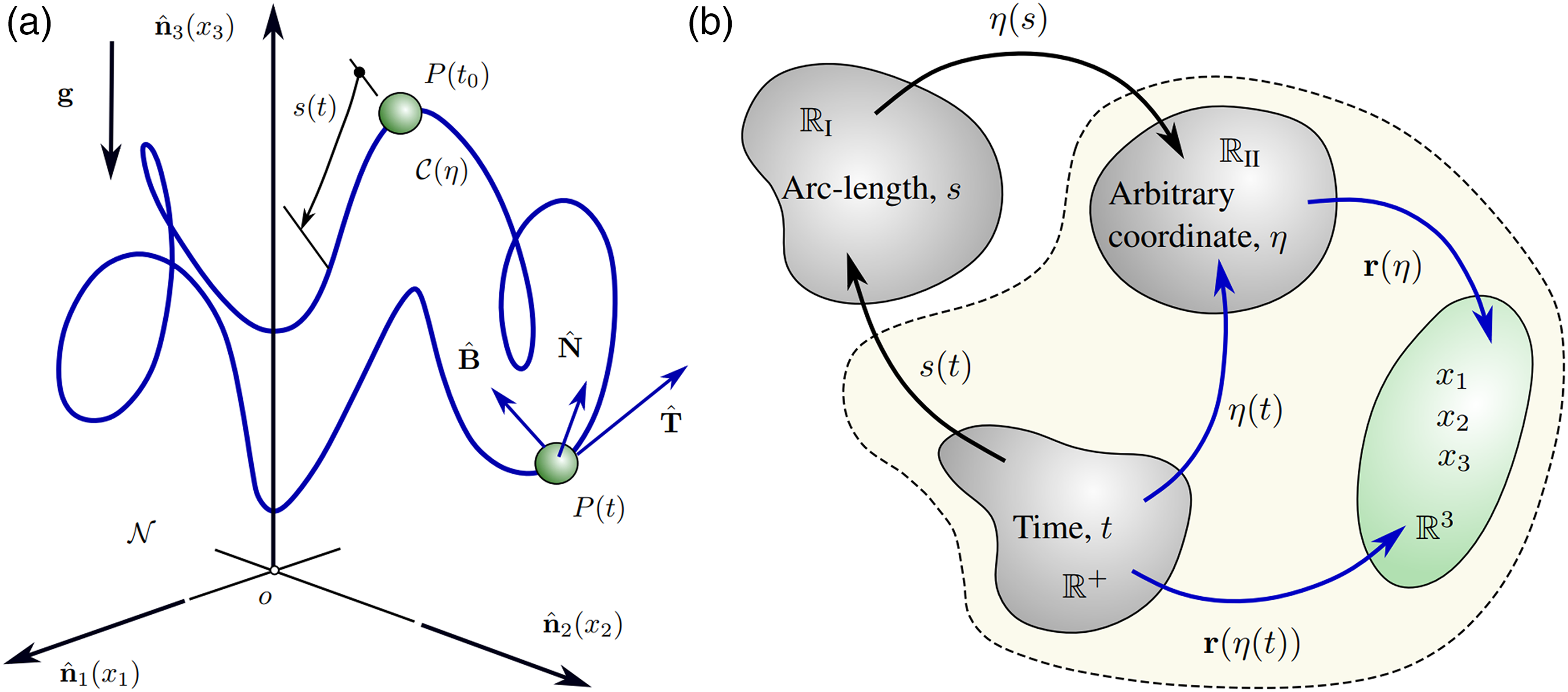
(a) Sliding bead, (b) Composition of functions.
The coordinate
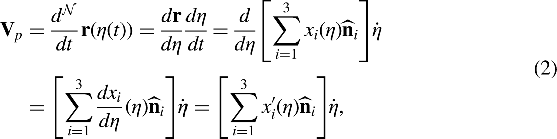
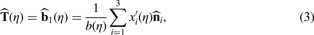
Under the fore-mentioned assumptions, the position vector of

As the main goal of this work is to use the knowledge gained during the first years at university, hereafter we assume that the curvature of

The next step is to obtain the equation of motion (EoM) of the particle

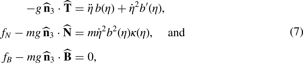
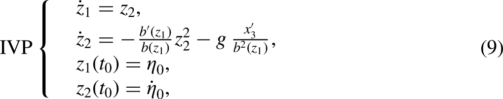
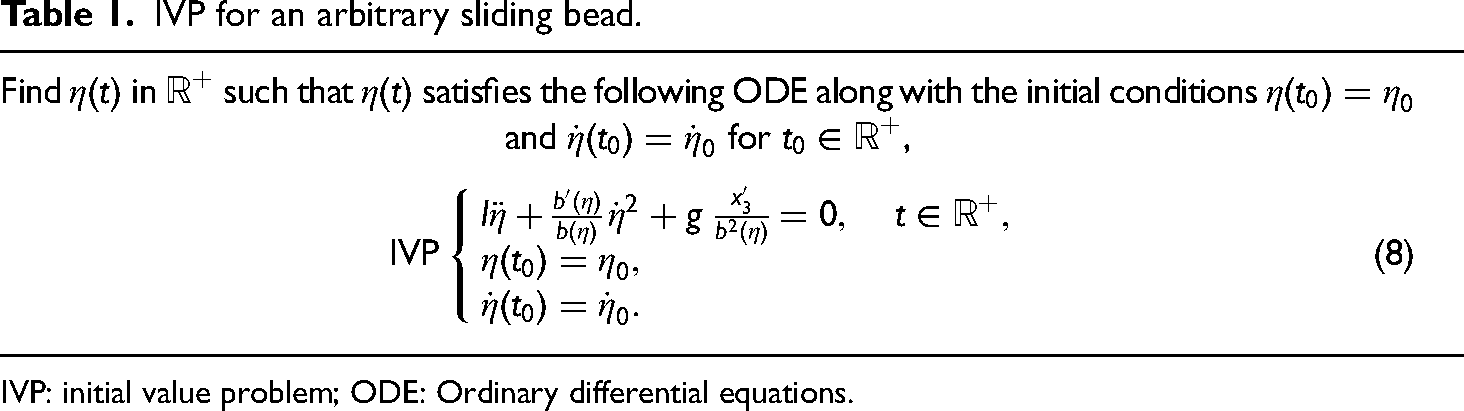
After some algebraic manipulations, the initial value problem (IVP) associated with a particle moving along a regular curve
As mentioned above, the dynamic equation for the sliding bead in (8) is a nonlinear second-order ODE. In general, it is not possible to find analytical solutions for this type of problem, so numerical techniques must be used to integrate the IVP.
19
Along this path, we define the auxiliary variables
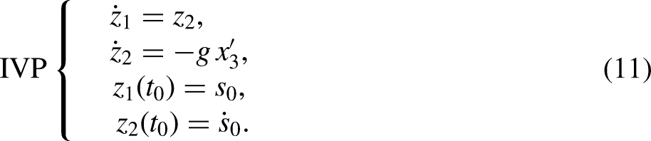
Phase portrait analysis
Let us set (11) equal to zero, i.e.,
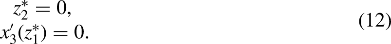
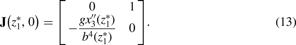
Stability analysis through linearization
One possible way to analyze the stability behavior of the system is to linearize around each equilibrium point. The matrix associated with the linear system is the Jacobian matrix, which at the equilibrium points takes the following form,
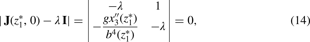
If If
In addition, it is possible to show that by incorporating viscous damping into the system the nature of the saddle points is not modified at all, while on the other hand the centers become asymptotically stable nodes or spirals depending on the added damping coefficient.
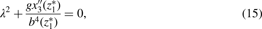
Stability analysis through energy
Besides the linearization-based approach introduced above, the stability of the fixed points can be analyzed through considerations about the energy of the system. The total energy

This finding can be justified by taking an interval


Potential energy around a local minimum.
Next, knowing that

Study case
As an example, we consider the curve given by (see Figure 4(a)),
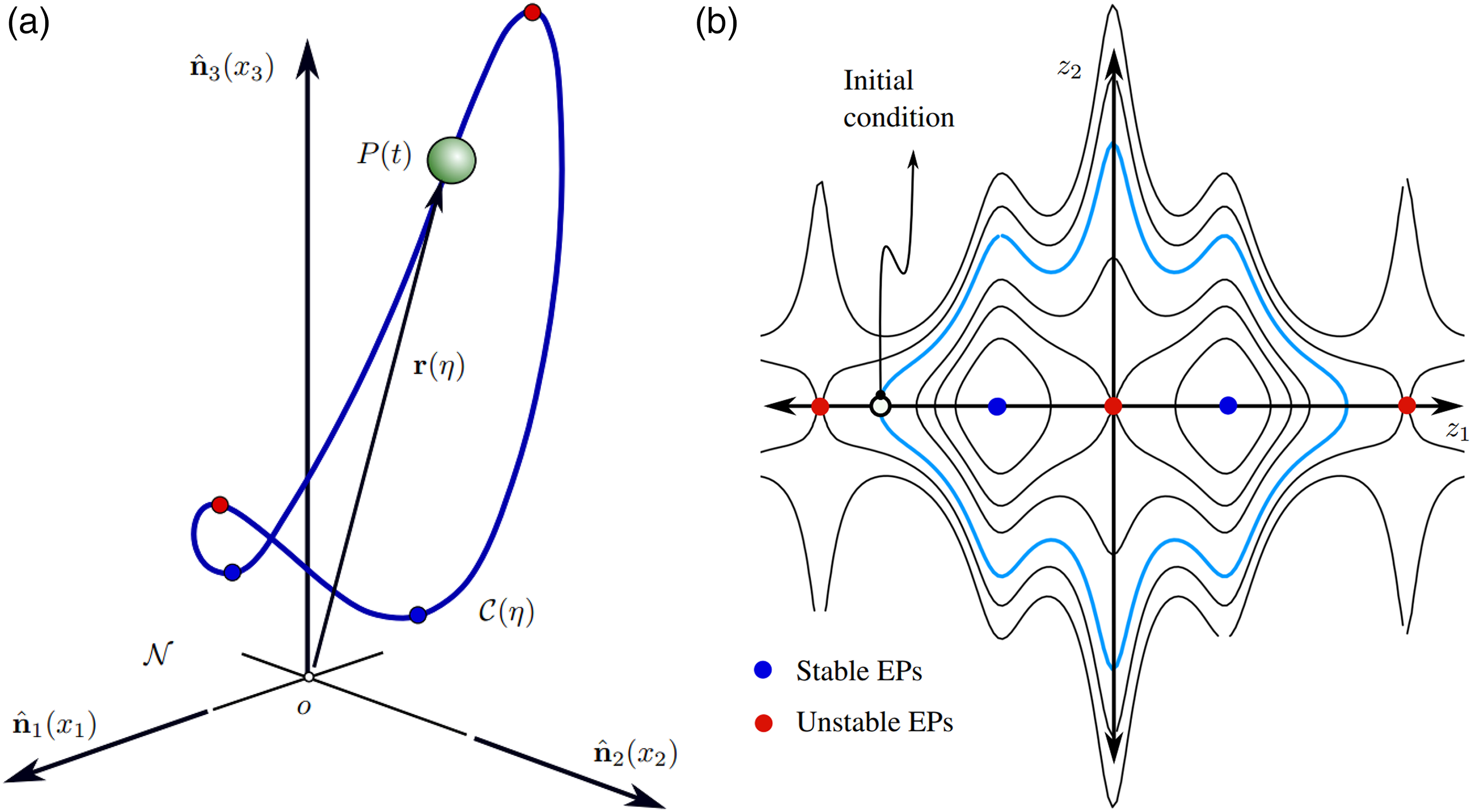
(a) Trajectory of the sliding bead, (b) Phase portrait, where EP stands for Equilibrium Point.
It is clear from Figure 4(a) that it has two local maximums associated with unstable critical points and two local minimums associated with stable critical points. Furthermore, the phase portrait in Figure 4(b) allows us to get some insights into the system by observing the equilibrium points as well as some trajectories. Since the system is conservative, such trajectories were computed from the level lines of the total energy as proposed in Strogatz. 20 Blue circular markers represent stable equilibrium points, while red circular markers represent unstable points. The light blue curve shows the trace of the solution for the initial condition indicated with a white marker. Such initial condition corresponds to the position of the particle in Figure (4(a)).
The use of animations of the physical system (simulation) is another powerful alternative to assimilate the new concepts acquired during the development of the project. In Bossio21,22 the student can find animations for the system without and with friction, respectively. In addition, the student can use software tools such as Pplane 23 and Geogebra 24 to deepen and improve their understanding of the behavior of such dynamic systems. A snapshot of the applet implemented in Geogebra is shown in Figure 5 with an animation of the bead sliding over the curve and the corresponding phase plane. By means of the green sliders on the right, it is possible to modify the initial conditions for the sliding bead. In Bossio 25 the reader can also find the implementation in Geogebra of the system presented here.
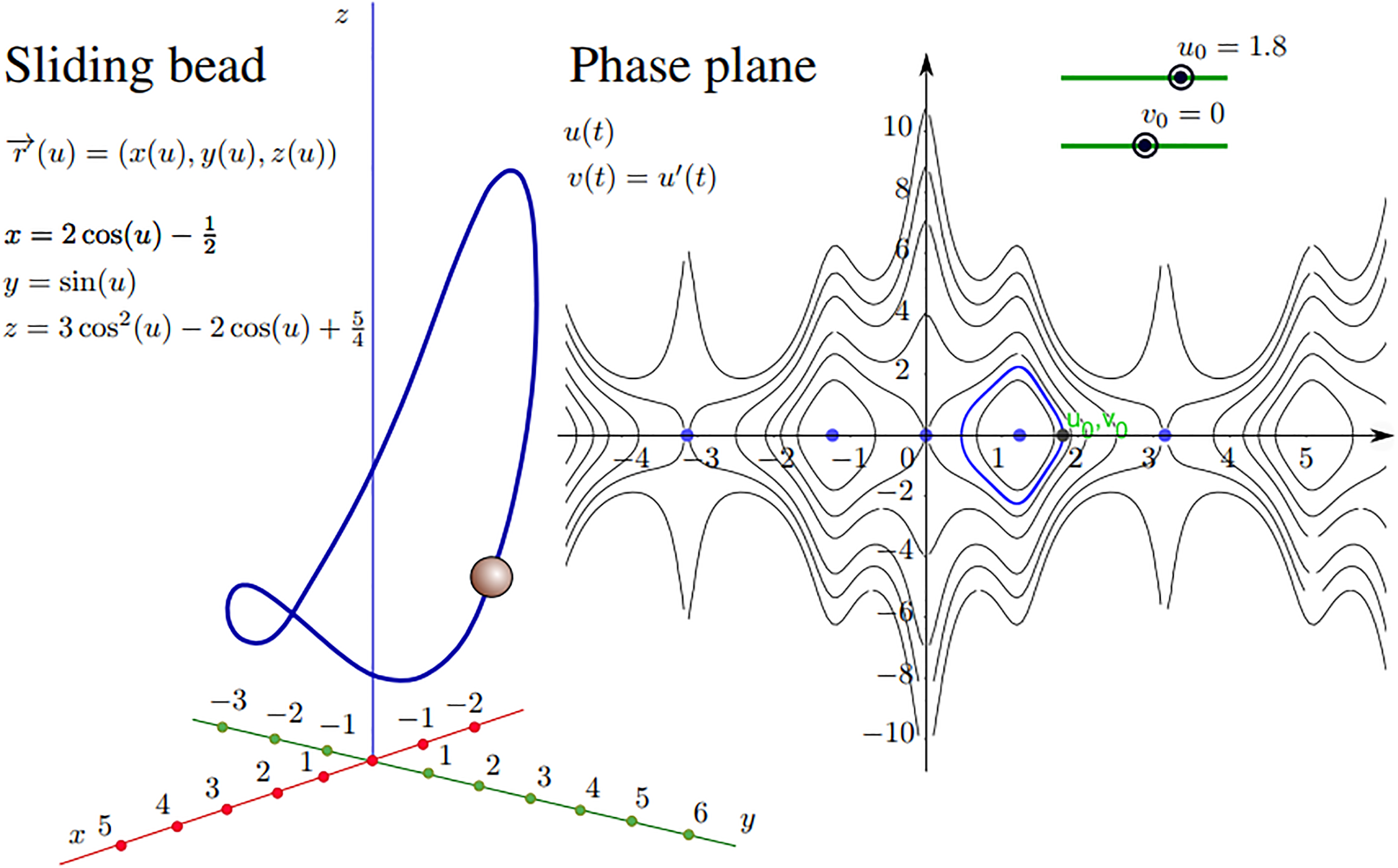
Applet in Geogebra for a sliding bead. 25
Numerical simulations
At this stage, the aim is to reinforce skills associated with those competences framed in computation. To this end, we propose to develop a computational-based tool to numerically integrate the nonlinear IVP stated in Table 1. Currently, there are several high-level script-based languages options well-suited for teaching purposes, such as: Matlab, GNU-Octave, Python, and Julia, among others. Here, we adopt Matlab due to mainly three reasons: Implementation simplicity, a well-established language for over two decades, and the ability to use the Simulink add-on to explore model-based designs.
IVP for an arbitrary sliding bead.
Classic numerical integration of the EoM
According to what is generally established, a numerical solution to the IVP (9) is understood as a procedure for finding approximate values
Among the large variety of numerical schemes to solve initial value problems, the specific selection of an integrator relies on the stability and stiffness of the ODE, as well as, the precision that one wants to achieve in the solution.
Regarding stability, we can distinguish between stability of the ODE itself and stability of its numerical solution. Roughly speaking, if the members of the solution family for an ODE move away from each other with time, then the equation is said to be unstable; but if the members of the solution family move closer to each other with time, then the equation is said to be stable. From a numerical point of view, we can even mention two other basic notions of stability:
The first notion of stability is concerned with the behavior of the numerical solution for a fixed value A second notion of stability is concerned with the behavior of the solution as It contains different time scales, i.e., some components of the solution decay much faster than others. The step size is controlled by stability requirements rather than by accuracy requirements. For a linear problem, all of its eigenvalues have negative real part, and the stiffness ratio (the ratio of the magnitudes of the real parts of the largest and smallest eigenvalues) is large. The eigenvalues of the Jacobian
The concept of stiffness is crucial in the numerical scenario; however, it is hard to define and has given rise to various attempts to describe it. According to Fasshaver,
26
a problem is stiff if:
Numerical schemes to integrate IVPs can generally be classified into two main types: (a) single-step methods, and (b) multi-step methods. The former, also called self-starter methods, estimate the solution
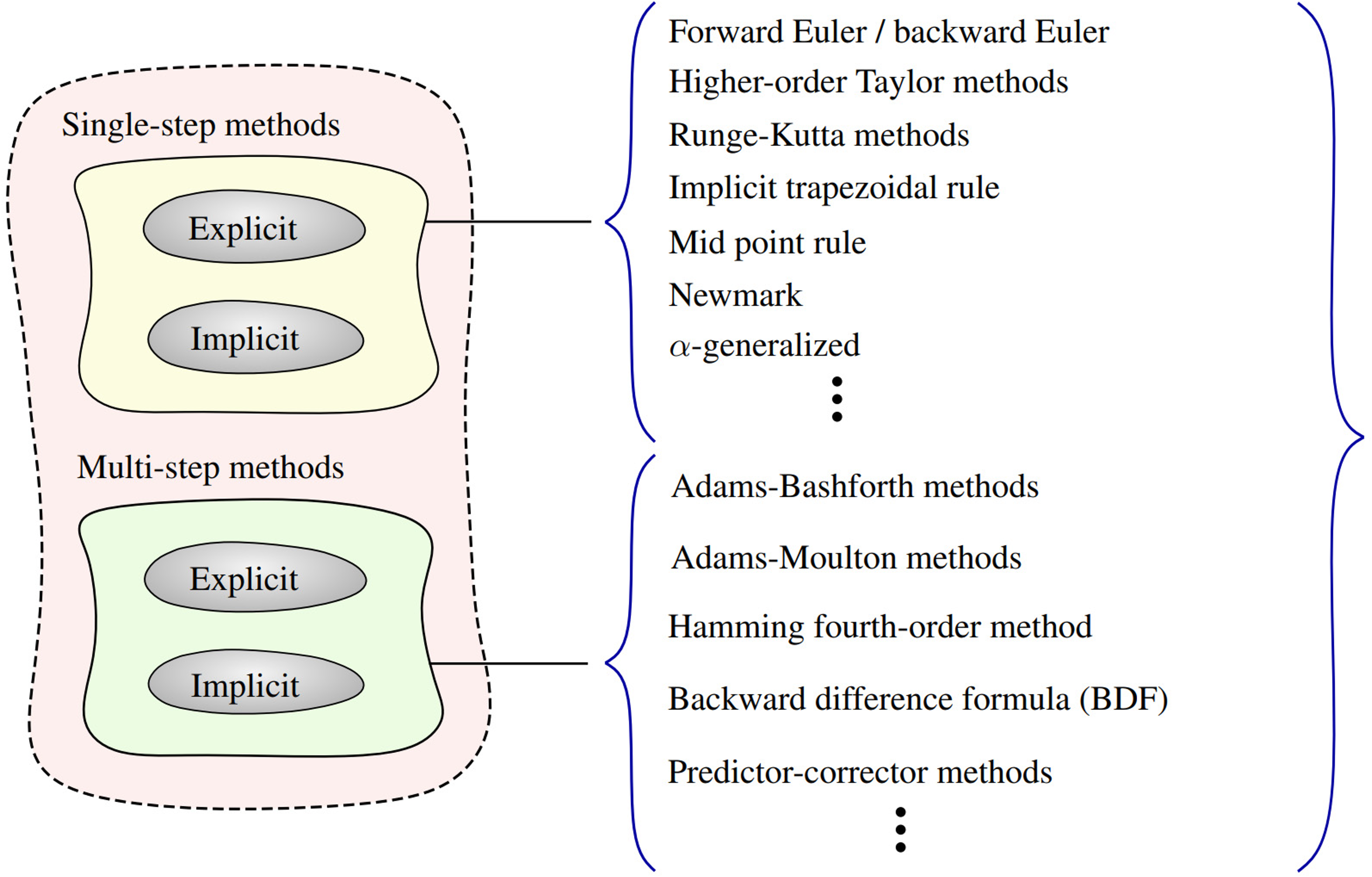
Classification of numerical methods to solve initial-value problems.
Unlike the explicit methods, implicit methods approximate the solution of a given IVP by considering the current state of the dynamic system,
In order to gain some competence in the use of numerical integrators as well as their coding, we present below some numerical simulations related to the dynamic model developed in the section on modeling. We consider here three different integrators: the Forward Euler method, the backward Euler method, and a RK (2,3) pair method implemented in Matlab via the intrinsic function ode23. The formulas for these schemes are given by:
Forward Euler (explicit): Backward Euler (implicit): RK (2,3) (ode23, Matlab): implementation of Bogacki and Shampine.
27
As mentioned above, implicit schemes to integrate (9) result in a set of nonlinear-algebraic equations, which must be solved iteratively at each time step until a convergent solution is reached (i.e., “dynamic equilibrium” is satisfied up to some extent). In this context, such equilibrium is understood as the balance, at each time step, between external forces and inertial forces.
Backward Euler formula can be rewritten as 

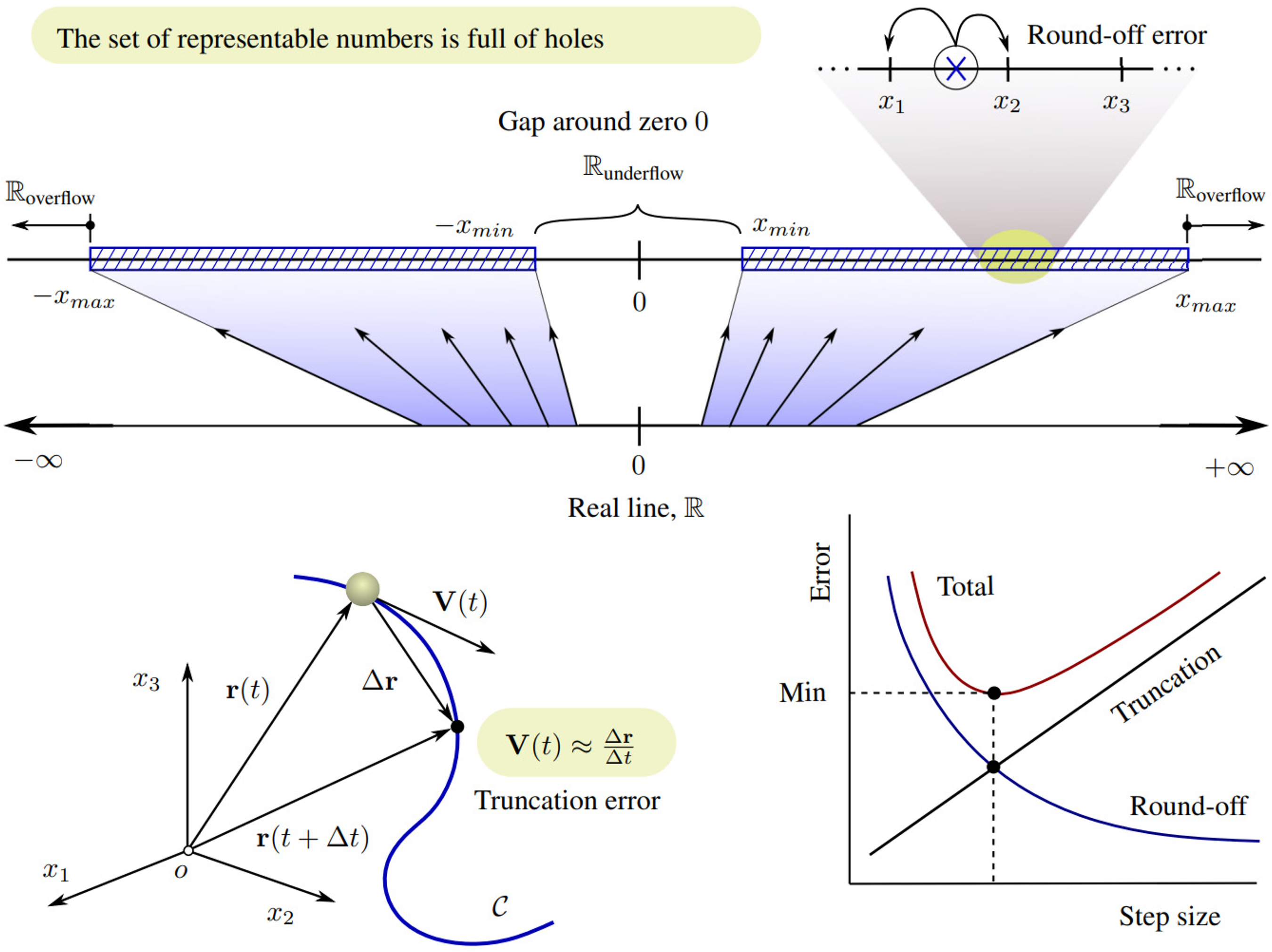
Schematic of round-off errors and truncation errors.
For numerical simulation purposes, we adopt the same curve used as an example for the stability analysis. In addition, the simulation data is: gravitational acceleration
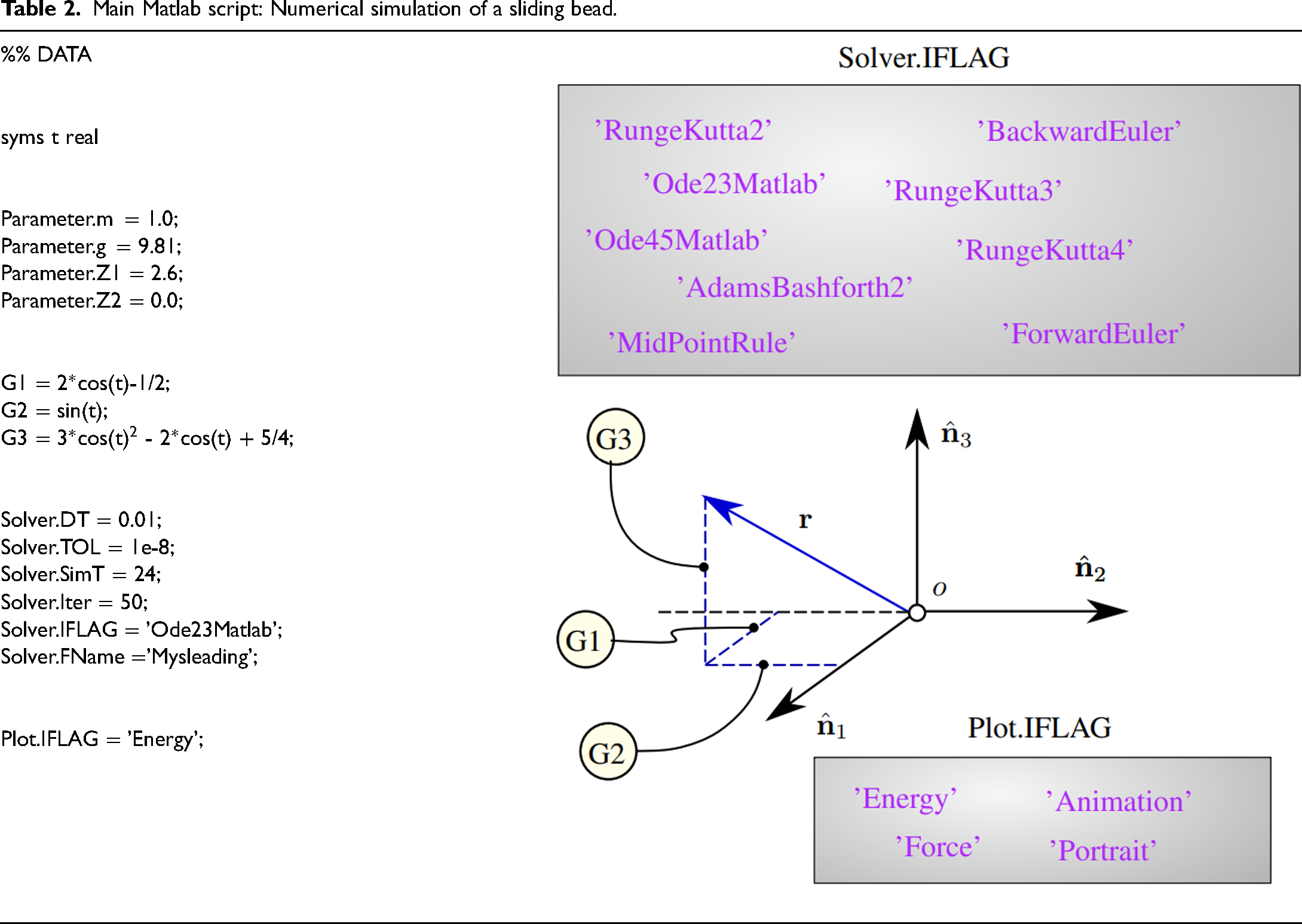
In Table 2 we present a snapshot of the main script of a Matlab-based computer code for the simulation of a sliding bead, where all the necessary input data is specified. 28 The structure Parameter plus the variables G1, G2, and G3 contain all the input data associated with the problem, while the structure Solver contains all the solver parameters. Finally, the structure Plot allows to specify the output plot desired by the user.
In Figure 8 we present some numerical results obtained by using the integrators proposed above. It should be noted that the system considered here is conservative and therefore the total mechanical energy must be constant for all time. On this basis, the energy plots in Figure 8 allow us to visualize how the different numerical schemes perform over time.
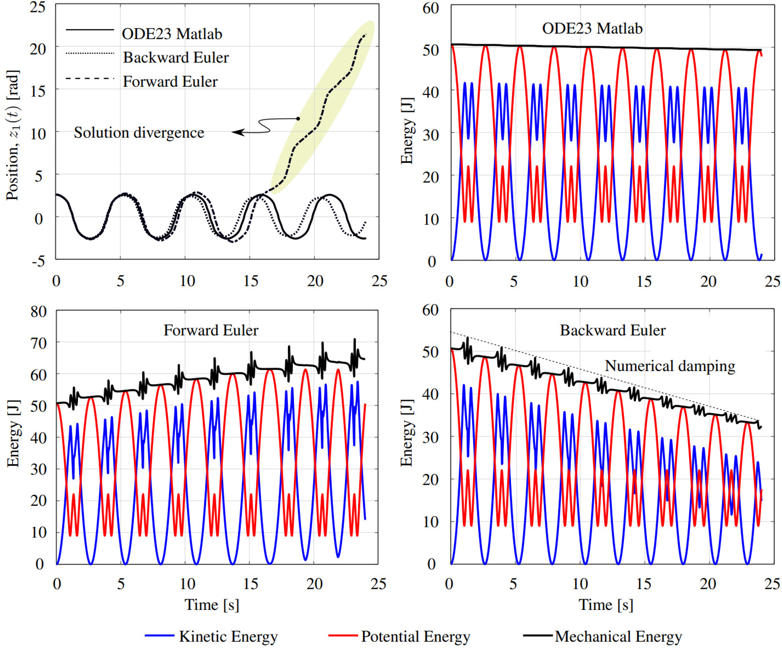
Position time series and energy (kinetic, potential and total) obtained by using the three proposed numerical integrators (
For
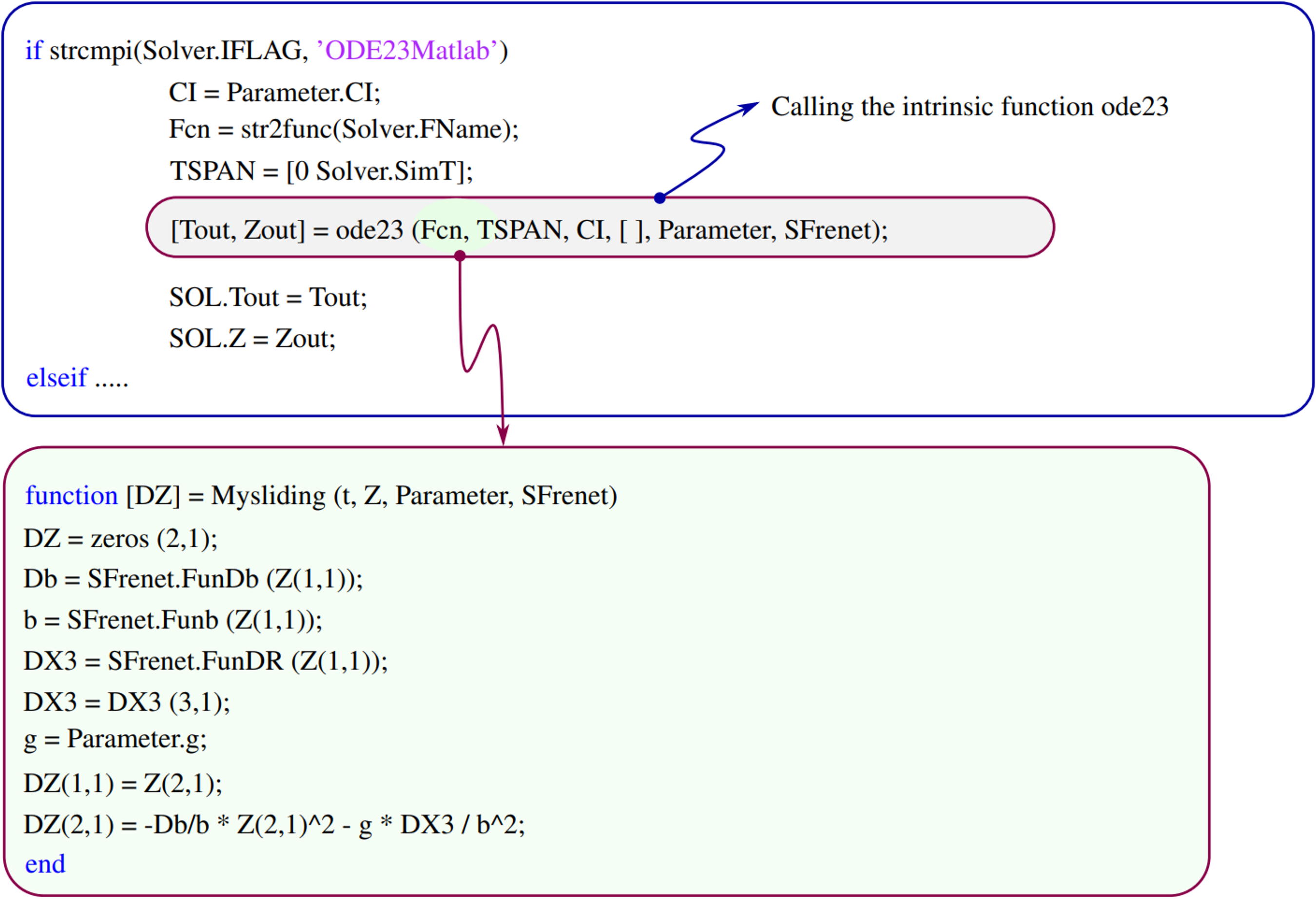
Intrinsic function ode23 Matlab code.
As mentioned above, the truncation error is proportional to the time step size. Therefore, a common strategy to reduce such an error requires reducing the time step. It is worth mentioning that for linear ODEs, the stability region associated with both forward and backward Euler methods are well known; consequently, an appropriate time step can be selected to achieve convergence. However, for nonlinear ODEs, the stability regions cannot be determined in general, and an adequate time step simulation relies mainly on trial and error procedures.
Figure 10 presents the time series of the restraining forces and energy, as well as a portrait diagram obtained using the backward Euler method with a significantly smaller time step. As can be observed, there is “almost no” dissipation in the energy curve. However, to achieve a sufficiently stable solution by using first-order schemes, the time step was decreased by 100. i.e.,
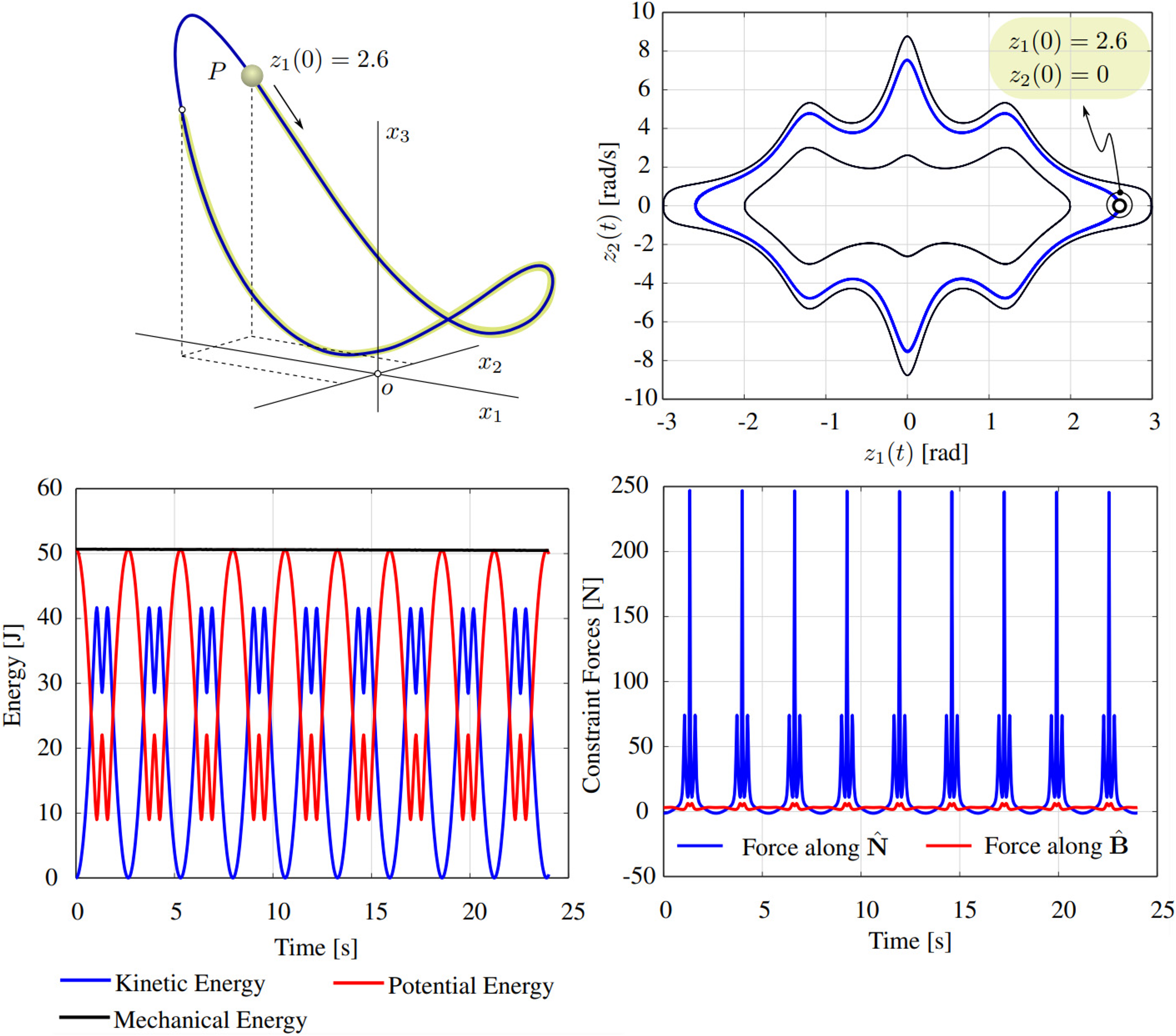
Portrait diagram, energy, and constraint forces obtained by using the backward Euler implicit scheme (
Another interesting point in analyzing mechanical systems is knowing the constraint forces acting on a body while it is moving. According to (7), the force magnitude along the binormal direction is simply
Integration of the EoM by using Simulink
Simulink is a graphical programming environment for Matlab. This is widely used in several fields of engineering, such as automatic control, digital signal processing, model-based design, and multi-domain dynamic system simulations, among others. For this reason, the development of skills with it is in many cases necessary to perform in the professional field. In Figure 11 the block diagram corresponding to the sliding bead model is shown. From the first integrator on the left, indicated with
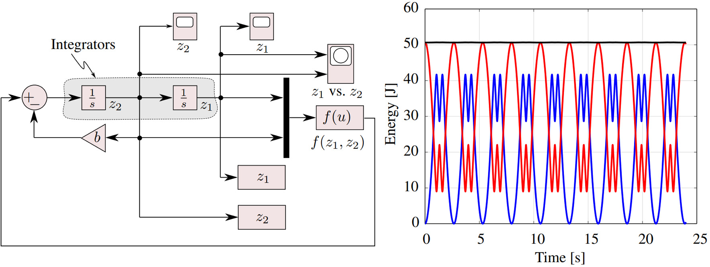
(Left) Simulink model, (right) energy plot, blue for kinetic energy, red for potential energy and black for total mechanic energy.
Analysis of the EoM by using Pplane
Pplane is a tool developed in Matlab to analyze autonomous planar systems in the phase plane. 29 This interactive tool allows to analyze systems of second-order ordinary differential equations. In Figure 12 can be seen the setup window where the equations system and parameters are entered. The display window shows the phase plane for the analyzed sliding bead model. For the numerical solution, the ode23 solver was used. The equilibrium points are shown in red. Finally, at the bottom left, the result of the linearization of two of the points, a minimum and a maximum on the curve, are shown.
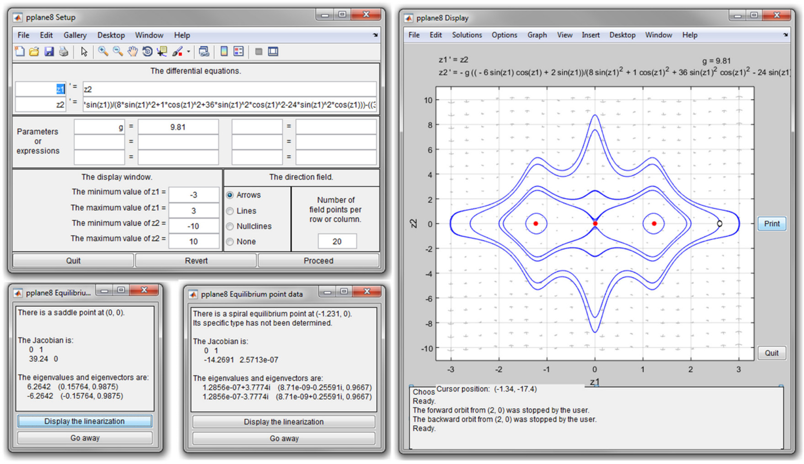
Pplane graphical-user interface.
Integrative project implementation
In this section, we briefly describe some aspects of the proposed integrative PBL project for the sliding bead. The integrative project we describe here is to be thought as an elective bachelor’s final project with 3 credits in the 6th semester for the bachelor in mechanical engineering, which aims to introduce the student to the field of computational mechanics. This project is not intended to become a compulsory undergraduate course with standard evaluation criteria.
The implementation of this PBL-based project proposed here serves as a step-by-step guide to some extent. According to the authors’ long experience teaching other courses in South America and Europe, the provided implementation guide lays a solid basis for its realization.
Through this project, we expect, as a main goal, that students acquire some insights in the field of computational mechanics and develop, at the same time, critical thinking and decision-making skills. To do this, we pursue the following specific learning objectives:
Articulate knowledge from other courses about the problem to be solved; Create questions, and propose solution strategies; Identify material of study; Reinforce and acquire new concepts related to dynamics, mathematical procedures to numerically solve ODEs, and coding skills, among others; Encourage discussion on such concepts within the working group and decide on the best possible way forward; Development of numerical simulations by using codes developed by themselves; and Preparation of reports.
Among the various aspects associated with a PBL approach, the teaching methodology, assignments, and assessment criteria are some of the most important, and therefore, they are the focus of discussion in what follows.
First, the integrative project will introduce students to the world of computational mechanics and why such a topic is important nowadays. Students will then be briefed on what a PBL problem is and its underlying methodology to ensure that they understand the process and what experiences they will face during the project. For the rest of the project, we will use a standard teaching approach, commonly used in PBL courses, as follows
30
:
Introducing the SBP, the resulting wide-ranging individual research that is expected to help clarify the problem, and the exposure to lecturer-prepared introductory material; Forming groups of students with, on average, three-to-four members. Group work allows the students to develop/reinforce extra competences such as to incorporate personal skills into a team, identify and organize group tasks, and to engage in shared decision-making; Analyzing the problem, elaborating questions to guide the learning, and laying out the goals expected from this integrative project; Proposing a solution strategy that should emerge as a teamwork effort; Perceiving gaps in the current students’ background (mathematics, mechanics, and computation). They can be noticed as the difference between the current students’ knowledge and potential future knowledge that may be needed to successfully address the sliding bead integrative project; Identifying the sources that contain the theoretical or practical information needed; Reinforcing and gaining new concepts on an individual level as well as a team effort; Setting goals and allocating resources within each group; Applying new knowledge to solve the different stages of the SBP; and Presentation, assessment, and reflection on the process and solution.
Although the phases presented above can be seen as a sort of sequential list to follow throughout the integrative bachelor project, some of them will be repeated during the project timeline as different questions or objectives of the project are addressed (phases 5 to 9). As the group progresses through the resolution, new knowledge and/or tools will be needed, which may not be apparent from the very beginning. In Figure 13 we present a diagram to illustrate the teaching methodology we adopted for the proposed integrative sliding bead project.
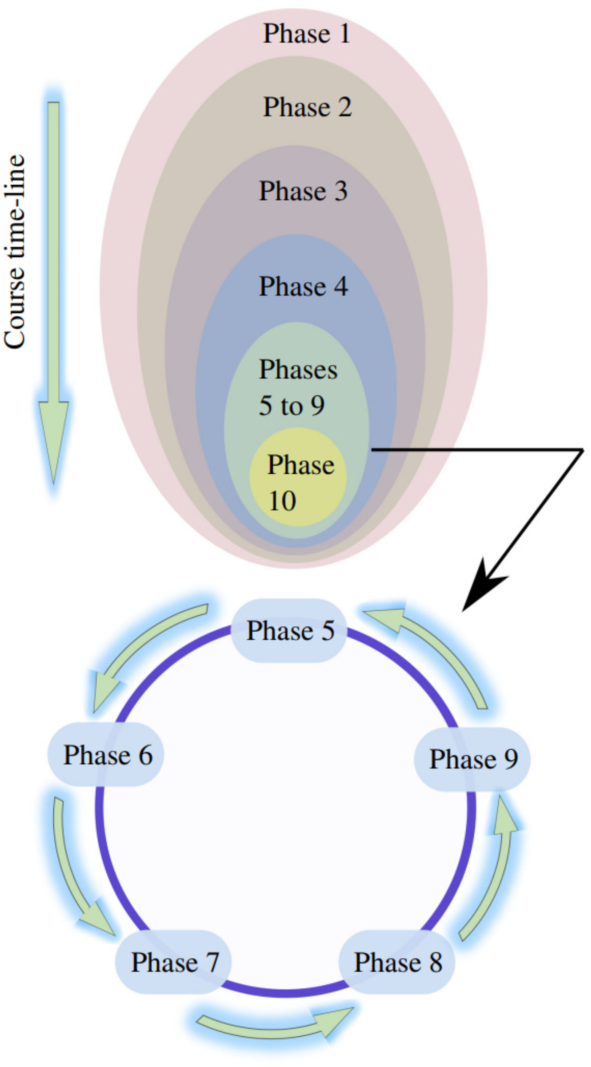
Teaching methodology.
In this work, the assignment to be delivered to the students consists only of the integrative bachelor project which meets all the features of the SBP. As mentioned before, such a problem has a substantial richness from a theoretical and practical point of view. Moreover, this problem represents an excellent starting point to study many other problems that arise in the real world, such as: roller coasters, design of slides in water parks, Ringette trajectories, and a considerable number of different devices in the industry, among others.
In Table 3 we present a tentative statement for a potential assignment to be used in this integrative project.
Main Matlab script: Numerical simulation of a sliding bead.
Tentative assignment.
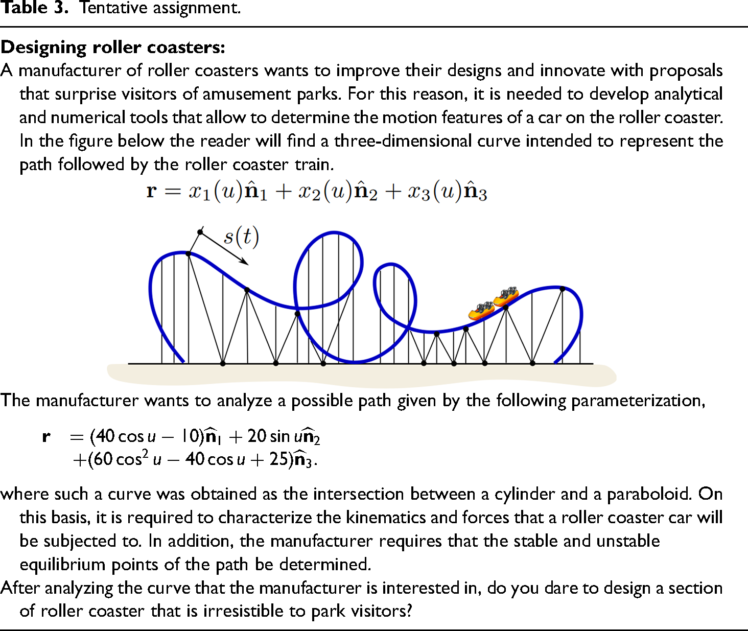
When designing a PBL problem, care must be taken to meet certain features that guarantee a solid learning for the student and allow the planned competences to be incorporated. In this sense, the proposed assignment largely meet these characteristics, which can be listed as follows:
Feature 1: Genuine problem. The problem posed in this case is based on real life, the roller coaster is an entertainment known to most students. Feature 2: Integrative problem. The roller coaster problem contains a large amount of concepts already acquired by the student as well as new topics to be incorporated. Feature 3: Complexity. PBL problems must have a certain level of difficulty; in other words, they should not be limited to a single solution. The roller coaster is not a routine problem such as those typical ones solved in the classroom. It demands research and the use of different tools. It is not a closed problem either, since students are encouraged to generate original proposals from the tools and skills acquired through the project course. Feature 4: Teamwork. The roller coaster problem is an excellent project candidate to be addressed by a group of students. The complexity of the problem and the multiple skills required for its solution make cooperation among students extremely necessary.
Finally, we discuss how the sliding bead integrative project will be assessed. It is planned to implement strategies at two levels. The first one is related to the assessment of the project outcome achieved by the group. The second level of assessment is related to the performance of each student within the group.
The total mark for every student is broken down as follows:
On one hand, groups will be assessed in the following areas ( Identify new concepts from mathematics, mechanics, and computation needed for the project. A plan of approach for developing the answers/tools required by the PBL assignment. Detailed report of the tasks undertaken as part of the solution process. Detailed minutes of the group meetings outlining the tasks developed, their distribution, and the percentage of completion of them. EoMs of a roller coaster car, numerical tools to study its equilibrium points, code to carry out numerical simulations of the car moving along the roller coaster. Versatility of the tools developed to study other configurations. Quality of the final report associated with the integrative PBL assignment.
On the other hand, the assessment of the students’ individual performance will be performed through documentation of the tasks carried out and peer assessment.
The first strategy requires the groups to meet at least once a week (documented in the form of meeting minutes). During each meeting it will be required that the students register the distribution of tasks to members, then at the following meeting, they will report on their progress on that task (
The second evaluation level will be based on a peer assessment of the group members of the other members of the group as well as an evaluation of their own contribution (last
All material and code generated to write this work were uploaded to a GitHub repository. 31 All future data, materials, statistics, and experience collected from a full implementation of this proposal will be duly uploaded to such a repository.
Relevance of the proposed model
The model presented in this work allows articulating concepts of mathematics, mechanics, and computation in engineering programs both horizontally and vertically. We understand by horizontal articulation that the articulation is to take place among complementary courses which are running in parallel. However, by vertical articulation, we understand that the articulation takes place over time building upon previously taught courses. In Figure (14) we show from which areas the proposed model can be addressed (red for physics, blue for mathematics, and green for computation). Several options are available, in physics for example we can use a two-dimensional simplified model to address concepts such as harmonic motion, potential and kinetic energy. In fact, the simple pendulum represents a particular case of the model presented here, when
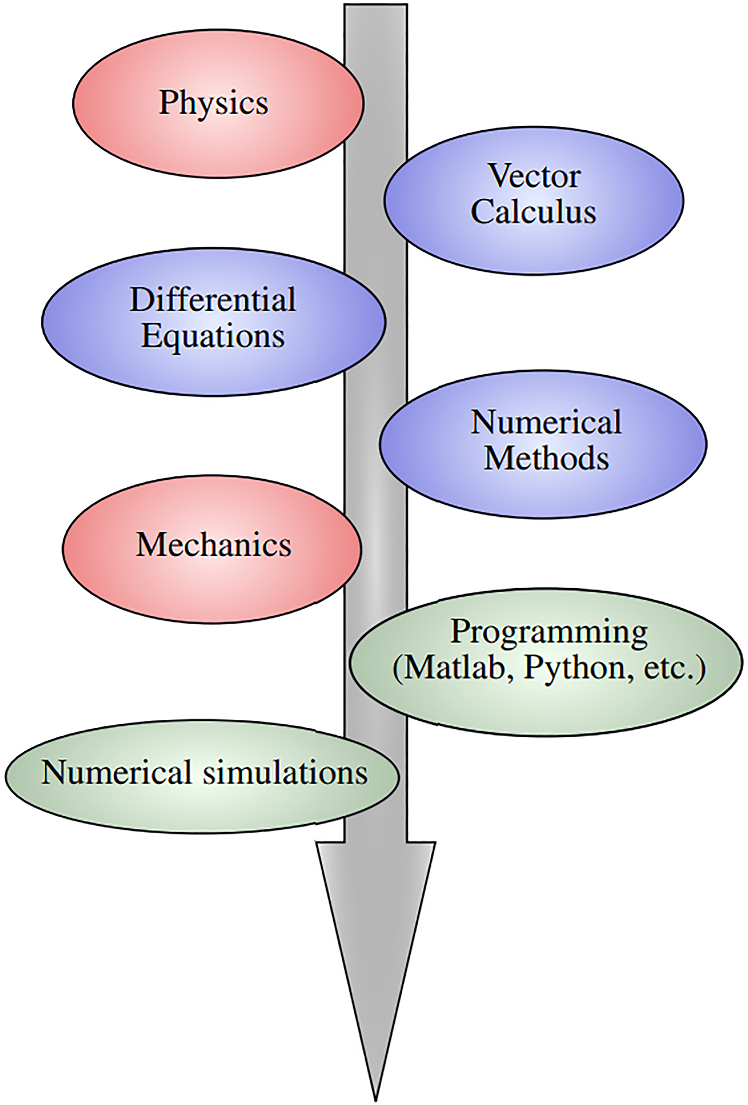
Possible areas to be articulated through the model proposed in this work.
In advanced undergraduate courses in mathematics such as vector calculus, we can use this model to study three-dimensional curves by means of the Serret–Frenet formulas as well as the acceleration components. 33 In differential equations this model is also useful since it allows to study the stability of nonlinear dynamic systems in a qualitative way. Along this path, Zill 34 proposes a simplified model to study the stability behavior of a sliding bead. In the context of numerical methods, the student can numerically integrate the IVP (9) to visualize the motion of the particle and thus complement the qualitative study carried out in courses of differential equations. To this end, the student also need to acquire/reinforce his programming skills in order to be able of carrying out numerical simulations, debug routines and/or functions, evaluate the quality of the results, and conduct verification and validation procedures.
The relevance of building an integrative project having the SBP as its core rests on the added value that it provides. The authors have included part of this problem in different basic courses such as vector calculus, rational mechanics, differential equations, and numerical methods, among others. During the teaching process we have noted several difficulties, mainly in those associated with the vertical articulation of concepts. In other words, students have problems in moving from problem analysis stage, modeling, use of mathematical tools already studied, and developing of new simulation codes, to drawing conclusions. Some of the questions that commonly arise are:
Why is the analysis of complex curves in space so important? What are the equations of motion for? Why are equilibrium points so important? What is a simulation? Is the numerical solution close to reality? How can the computer affect a numerical solution? What is V&V (verification & validation)?
Clearly these questions have arisen at different stages of different courses. In this sense, each basic course allows to address and answer one or two of these questions but fails to give a comprehensive understanding of what computational mechanics means. On this basis, the SBP allows agglutinating all the fields and moving through them interactively.
Conclusions
This educational work employed a PBL method to develop an integrative bachelor project suitable for: (a) reinforcing concepts gained in previous courses: (b) acquiring new competences in mathematics, mechanics and computation, and (c) providing means for the student to make a first incursion into computational mechanics. Because in PBL approaches it is the problem that drives the learning, in this work we have carefully selected, as the driving problem, the motion of a particle along a curve in space subject only to the action of the gravitational field. This dynamic problem enjoys an abundant richness from a mathematical and mechanical point of view in a way that allows the student to navigate among previous concepts and acquire new skills as well. For this, we used Newton’s second law along with Serret–Frenet formulas to describe, in an elegant and simplified way, the kinematics of the particle. Such a model can also be obtained in a simpler way in the basic courses from energy considerations or using concepts of Lagrangian mechanics in more advanced courses. Subsequently, we carried out a detailed stability analysis of the resulting equations of motion by using two different approaches: Linearization and energetic considerations. Next, we presented a detailed, but not exhaustive, introductory discussion of the time integration of EoMs, detailing the advantages and disadvantages of various numerical schemes and providing some queries for the student along the way. Finally, we established a brief discussion about how mathematics, mechanics and computation are articulated as the integrative project moves forward.
As a part of this project, we have also developed simulation and visualization tools to help the student incorporate new knowledge and challenge them to go one step further by developing their own numerical simulators. Such codes as Geogebra and the script listed in Table 2 are available on the web.
It is possible that this course could form the basis of a future field course, in addition to further supporting current research interests. We look forward to using this teaching approach in future courses.
Footnotes
Declaration of conflicting interests
The author(s) declared no potential conflicts of interest with respect to the research, authorship, and/or publication of this article.
Funding
The author(s) received the following financial support for the research, authorship and/or publication of this article: This work was partially supported by the Universidad Nacional de Río Cuarto (UNRC), Consejo Nacional de Investigaciones Científicas y Técnicas (CONICET), and the Bergen Offshore Wind Centre (BOW), Norway.
Data Availability Statement
Data sharing not applicable to this article as no datasets were generated or analyzed during the current study.