Infrared video imaging for in-line evaluation of oxide descaler performance on steel strips

Abstract

In-line assessment of descaler functionality was conducted through use of high-speed infrared (IR) video imaging of moving steel strips following laminar cooling. IR temperature measurements were obtained for fifteen (15) steel strips at a mill location between laminar cooling and coiling. Anomalous temperature values were observed in the IR images and were attributed to the presence of surface oxides. The location and spacing of these oxides were quantified using an outlier detection method consisting of a Gaussian process and Gaussian mixture model. Validation of the outlier detection method was done through comparison of both the morphology and emissivity of oxide regions to those reported in literature. The oxides were predominately located at the mid-width of the strip, while their transverse spacing correlated well with the descaler nozzle spray patterns. The transverse spacing and location of these oxides indicates that the reheat furnace and/or rough-rolling entry descaler was operating with reduced functionality. Total fraction of surface oxides was also shown to be correlated with the amount of silicon in each strip and the total roll reduction.

Keywords

TMCP machine learning IR imaging oxides descaler steel

Introduction

Thermomechanical controlled processing (TMCP) is commonly used to produce high strength low alloyed (HSLA) steels for the oil and gas and automotive industries. TMCP consists of four major process steps including homogenisation ( $\sim$ 1200 $\circ$ C for 2 h), rough rolling ( $\sim$ 1100 $\circ$ C–1200 $\circ$ C), finish rolling ( $\sim$ 800 $\circ$ C–900 $\circ$ C) and laminar cooling. The relatively high temperatures associated with homogenisation and rolling can result in the formation and growth of surface oxides.¹ It has been observed that the presence of these oxides can adversely influence the strip microstructure and mechanical properties.^2,3 While the mechanism by which surface oxides affect microstructure is an area of active research, some have suggested that it can be attributed to a shift in the boiling curve during accelerated cooling.^3,4 By changing the Leidenfrost temperature, the presence of oxides may cause the surface boiling mechanism to change from the thin film regime to the transition boiling regime,^5,6 which could result in a significant increase to the local cooling rate⁴ possibly forming local hard zones.^3,7

Oxides formed during TMCP can be classified as primary, secondary, or tertiary.^1,8 Primary oxide scale is formed during homogenisation and generally exhibits a strong interfacial bond with steel.¹ A secondary oxide scale forms and grows during the rough rolling schedule. Finally, a tertiary oxide scale can form during finish rolling, cooling, and coiling. The scale that forms in each TMCP stage is generally a layered structure consisting of an inner layer of wüstite (FeO) overlaid with magnetite (Fe $_{3}$ O $_{4}$ ) and an outer layer hematite (Fe $_{2}$ O $_{3}$ ).^9–12 For silicon (Si) containing steel, fayalite (Fe $_{2}$ SiO $_{4}$ ) can also form between the steel and wüstite layers.¹³

Pressurised water descalers are typically used to remove surface oxides from steel strips. These descalers consist of flat-fan nozzles connected to a pressurised water header and are arranged in banks across the width of the strip. The arrangement and positioning of each individual nozzle in a bank is pre-set to maximise surface area coverage and oxide removal.¹⁴ The descaler banks are located at specific positions in the hot strip mill including between the homogenisation furnace and the roughing mill and between the roughing mill and the finishing mill. Decreased descaling efficiency has been observed^15,16 and is attributed to nozzle spray interaction and obstruction. In addition, rolling mill parameters and steel chemistry^17,18 can influence the functionality (i.e. ability to remove oxides) of the descalers on a hot strip mill. Oxides that are not removed prior to rolling deformation can exhibit increased adhesion to the steel surface and resist removal by subsequent descaler banks.¹⁹

As the strip traverses the ROT from the finishing stands, it goes through various cooling mechanisms as a result of its interactions with both air and water. In the regions where there is no exposure to water, the primary cooling mechanisms are convection and radiation. Directly underneath each header nozzle, multiple cooling mechanisms are taking place, namely single phase convection, nucleate boiling, transition boiling, and film boiling. These various cooling mechanisms result in a non-uniform surface temperature of the strip. Studies such as Guedia Guemo et al.²⁰ illustrate the influences of these mechanisms on the subsequent strip surface temperature profile.

The use of machine learning algorithms for image analysis is a well established practice.^21–23 Some studies have combined machine learning with thermography for the detection and classification of defects.^24–26 Generally, these models consist of a preprocessing step followed by clustering. The purpose of preprocessing is to clean the data and prepare it for effective clustering. Examples of these types of models are KNNimputer, kernal ridge regression, and Gaussian processes (GPs). Many clustering models exist, but some of the most common are K-means, DBSCAN (density-based spatial), and GMMs. In this work, a combination of GPs and Gaussian mixture models (GMMs) was used. An overview of these methods is provided in Appendix A.

The ability to assess (and ultimately correct) the descaler functionality generally consists of visual assessment of the strip surface. This work combines in-line infrared (IR) thermography with statistical analysis to quantify the presence and location of surface oxides. A series of plant trials were carried out in which IR temperature imaging data was obtained from a hot steel strip mill at a camera position after laminar cooling and before coiling. For each steel strip studied, $\sim$ 200 IR frames (sequential images along the length of the strip) consisting of $\sim$ 327,680 pixels each were obtained. Each individual IR frame was digitised, and the location and spacing of potential oxides for the entire strip length was quantified using an outlier detection method consisting of a GP and a GMM. The GP was used to eliminate large, continuous temperature variations along the width of the strip. These large, smooth variations were unlikely to be caused by oxides, so their removal helped to prevent false positives. The difference in temperature between the GP correction and the original data was used to calculate emissivities, which were then clustered into components using the GMM. The morphology and emissivity of individual oxides in each IR image were analysed and correlated with known surface oxide shapes and values. Total fraction of oxides on each strip were then related back to chemistry and processing of the steel.

Materials and methods

Materials

Fifteen industrially hot rolled steel strips were analysed using IR thermography and are labelled S1 to S15. The strip thickness, homogenisation, rough rolling, finish rolling temperatures and the Si wt-% for each strip are shown in Table 1.

Table 1.

Strip processing parameters and chemistry.

Strip	Gauge (mm)	Homogenise ( $\circ$ C)	Roughingmill exit ( $\circ$ C)	Finishingmill exit ( $\circ$ C)	Si (wt-%)
S1	7.87	1284	1068	913	0.260
S2	10.97	1259	1130	894	0.060
S3	10.97	1259	1126	897	0.060
S4	10.97	1259	1136	909	0.060
S5	10.97	1257	1126	901	0.050
S6	10.97	1257	1126	890	0.050
S7	10.97	1258	1128	887	0.050
S8	10.97	1259	1128	920	0.040
S9	10.97	1259	1127	895	0.040
S10	10.97	1259	1130	894	0.050
S11	11.51	1284	1110	889	0.014
S12	11.51	1260	1103	892	0.017
S13	11.51	1222	1109	890	0.014
S14	11.51	1258	1109	890	0.014
S15	11.51	1255	1097	889	0.013

Methods

IR thermography

A Telops FAST M350 IR camera with a spectral detection band of 1.5–5.4 $μ m$ , sensor pitch of 15 $μ m$ and 20 mK NETD, was installed in parallel to the TMCP coiler pyrometer, as shown in Figure 1. By situating the camera in this location, the adverse effects of steam on IR measurements were minimised. The camera was positioned $\sim$ 3 m above the surface of the moving strip, producing a field of view of 1.8 m by 1.4 m and a pixel resolution of 2.7 mm by 2.7 mm. This resulted in each frame of the IR videos containing a total of 327,680 pixels/temperature readings. The speed at which strips traversed the ROT varied from 1 to 4 m/s, so the camera acquisition rate and exposure time were adjusted to capture all portions along the length. For all strips, an acquisition rate of 0.2 $s^{- 1}$ was used along with an automatic exposure time.

Figure 1.

Schematic diagram of camera placement in thermomechanical controlled processing (TMCP) process.²⁷

Validation and emissivity determination of IR measurements was done through comparison with the coiler pyrometer. The imaging software for the IR camera allows for defining regions of interest (ROIs) in the videos, where only the temperature profile contained in the ROI is recorded. By positioning the ROI close to the sampling region of the pyrometer, and matching both temperature profiles, the emissivity of the strip recorded was determined. Figure 2 shows a comparison of temperature profiles produced from the IR camera versus the pyrometer for S15, where an emissivity of 0.86 was shown to produce the best match. For all strips, the emissivity showed little variance with values of $0.845 \pm 0.015$ . The only exception to this was S1, which had an emissivity of 0.73.

Figure 2.

Calibration of S15 using an emissivity of 0.86.

Using the calibrated IR data, the mean temperature (Temperature measurements are presented as scaled temperature to obscure proprietary process data. Scaled temperature is calculated by dividing all measurements by the maximum temperature in the range.) and standard deviation of each frame was plotted as a function of distance along the length of the strip (Figure 3). The darker blue shading indicates one standard deviation in temperature with the light blue shading indicating two standard deviations in temperature. The large, consistent variation in temperature along the strip is attributed to the spatial variation in strip cooling.

Figure 3.

Scaled mean and standard deviation of each frame for S15.

The large temperature variation observed along the length of the strip (Figure 3) is illustrated for a single IR image frame (Frame 199 (199) for S15) in the colour coded temperature heatmap shown in Figure 4. The temperature of the strip was observed to vary from <600 $\circ$ C (dark blue regions) to 650 $\circ$ C. This complicated variation in surface temperature was observed for all the steel strips analysed and necessitated the development of statistical methodologies to provide quantitative data on temperature and its relation to surface oxides.

Figure 4.

Infrared (IR) video frame for S15-199. Colour bar indicates the scaled temperature.

Outlier detection

With abnormal temperature fluctuations present in the IR measurements, an outlier detection method was developed to isolate these regions. The developed method combined the techniques of GPs and GMMs. Through use of the GP, the true underlying temperature of the strip surface was estimated. With this, the emissivity of each pixel in the IR video could be calculated. These corrected emissivity values could then be clustered into distinct components. This section provides a comprehensive analysis of S15 while only the results for all other strips are presented.

Accounting for differential cooling

While IR thermography has been proposed for the inline detection of abnormally cold regions on strip surfaces,³ its applications are limited by its inability to account for variations in emissivity. This is especially relevant to TMCP, where oxides (scale) form throughout the process. As was shown by del Campo et al.,²⁸ the emissivity of an iron surface can increase dramatically as it oxidises. While the difference may not be as extreme for the unpolished steel in TMCP, it cannot be assumed that variations in surface emissivity are negligible. While two-colour pyrometers are capable of accounting for this variation, they are limited by the small region that they measure. Furthermore, as even small regions of oxidation have been shown to form localised hard zones,³ pyrometer-based monitoring systems may not capture these defects.

During the calibration of an IR camera, the emissivity of the subject is adjusted until the temperature observed by the camera matches its true temperature. If the true temperature is known for every pixel in the frame, this method can be inverted to transform an IR image into a map of emissivities. In the case of TMCP, the temperature of the subject (the surface of the strip) is much higher than the ambient temperature. By neglecting this ambient radiation, and assuming that the emissivity of the subject is constant within the waveband of the camera, equation (1) is derived.

ϵ_{corrected} = ϵ_{measured} \frac{\int_{λ_{1}}^{λ_{2}} λ^{- 5} (e^{h c / λ k T_{measured}})^{- 1} d λ}{\int_{λ_{1}}^{λ_{2}} λ^{- 5} (e^{h c / λ k T_{true}})^{- 1} d λ}

(1)

where

ϵ_{measured}

is the emissivity setting used during an initial measurement of

T_{measured}

T_{true}

is the true temperature of the surface.

h

and

c

are Plank’s constant and the speed of light, respectively.

ϵ_{corrected}

is the emissivity after accounting for the difference between the measured temperature and the true temperature.

λ_{1}

and

λ_{2}

are the lower and upper bounds on the waveband of the IR camera, respectively. The issue then becomes measuring the true surface temperature at every point in the frame.

To estimate the emissivity-independent surface temperature $T_{true}$ , some important features of the laminar cooling process are noted. First, cooling is applied by jets along the width of the strip; small variations in the spray velocity/pressure may result in cooling that is varied transversely, but not longitudinally. Consequently, it is not reasonable to assume that the true surface temperature is constant over a given frame.^29,30 However, variations in the true temperature should predominately occur transversely. Longitudinal temperature variations are, therefore, attributed to variations in surface emissivity, while transverse variations are assumed to be dominated by differential cooling imparted by ROT jets.

As temperature variations measured along the width of the strip were assumed to be dominated by real variations in the true surface temperature, these measurements were isolated through the use of a GP. This was done by disregarding the length index of each pixel, and fitting a GP to the resulting temperature-width data for each frame of the IR video. This is shown in Figure 5 for frame 199 of S15. The mean of the GP was taken as the true temperature ( $T_{true}$ ) for the entire frame, as is shown in Figure 6. By doing this for each frame, the gradual change in temperature measured by the pyrometer (Figure 2) can be accounted for without any assumptions about the longitudinal heat transfer characteristics. While this still neglects some intra-frame temperature variation, it should be noted that the pyrometer-measured variation within the length of a single frame is, on average, an order of magnitude smaller than the transverse variation observed by the IR camera.

Figure 5.

Gaussian process (GP) approximation of true temperature profile across the width of S15-199.

Figure 6.

Scaled true temperature ( $T_{true}$ ) for S15-199 estimated by the Gaussian process (GP) shown in Figure 5.

With $T_{true} \approx μ_{GP}$ , it was then possible to generate an emissivity map for each frame using equation (1). The temperature and estimated emissivity maps for S15-199 are shown in Figure 7.

Figure 7.

Surface plot of temperatures (left) and estimated emissivities (right) for S15-199.

This method was used in place of taking the average temperature along the width. While this is considerably more complicated, it has some advantages. First, the resulting mean temperature profile is smooth; there are no discontinuities and it is infinitely differentiable. This is a more accurate representation of the underlying system than a set of discrete averages. Second, this minimizes the number of assumptions about the shape of the true temperature profile, which eliminates bias that would be introduced by fitting a parameterised function to the data.

Clustering IR data

Stemming from the distinct components observed in Figure 4, a mixture distribution of emissivities was hypothesised for each strip. It was assumed that a finite number of factors influence emissivity, resulting in a probability density function modelled as a combination of multiple Gaussian distributions. Each Gaussian component represents a distinct cluster of data, which may correspond to variations arising from specific factors.

The number of components in the IR videos for each strip is unknown, so a fixed value was not predetermined. Instead, the Akaike information criterion (AIC) was employed to determine the optimal number of components. As the number of components in the GMM increases, the model fit improves, but the risk of overfitting also increases. AIC serves as a selection criterion to identify the model that achieves the best balance between goodness of fit and overfitting. Equation (2) defines the AIC for a given model, where $k$ represents the number of parameters (the number of components in the GMM), and $\hat{L}$ is the model likelihood.

AIC = 2 k - 2 \ln \hat{L}

(2)

A minimum of three components was assumed for each video. This was based on the observation of three distinct colours in the IR frames (Figure 4). An upper bound of 10 components was also assigned to minimise the risk of overfitting. For each strip, the data from individual frames were aggregated into a single dataset, to which equation (2) was applied. Figure 8 compares the fit of the GMM with the measured emissivity data and includes the individual Gaussian components.

Figure 8.

Gaussian mixture model (GMM) results for S15.

The optimal number of components was determined on a case-by-case basis by analysing the AIC curve. In most cases, the first or second elbow of the AIC curve was selected as the optimal value. However, for datasets exhibiting a smooth curve without a clear elbow, the maximum component value of 10 was used. For example, based on the AIC curve of strip S15, 10 components ( $k \in {1, \dots, 10}$ ) were chosen for clustering.

From the model results (Figure 8), the highest Gaussian component was assumed to correspond to the emissivity associated with oxides on the surface. To isolate all oxides from the IR videos, a threshold value based on this Gaussian component needed to be chosen. Since each Gaussian component provides the probability that a given emissivity value belongs to that component, the threshold was set at the point where the probability of the second-highest component approaches zero (the right tail). This approach ensures that only the emissivity values belonging exclusively to the highest component are isolated. Using this method, emissivity values for the oxide components ranged from 0.76 to 0.92, which was in agreement with previous studies.²⁸ With these emissivty thresholds, each frame in the IR videos were analysed.

Oxide morphology

The morphologies of all oxides was analysed. Figure 9 shows the oxide morphologies for S15-199 (black regions). Each oxide displays a smooth tear drop shape, which correlates strongly with primary and secondary scales observed during rough rolling.¹ These morphologies were similar among all the strips analysed.

Figure 9.

S15-199 oxides and their morphologies.

Results and discussion

Oxide spacing

For the TMCP line under investigation, six descaler systems are employed. Descaler 1 is positioned between the reheat furnace and the roughing mill. Descaler 2 is located at the entry to the roughing mill. Descaler 3 is situated between the roughing mill and the coiling box. Descalers 4 and 5 are between the coil box and finishing mill. Lastly, descaler 6 is in the finishing mill, between stands 1 and 2.

Figures 10 and 11 present the y-coordinates of the detected oxides for select strips. In each case, regions of high and low concentrations are evident from the primary maxima and minima in the histograms on the left side of each plot. Additionally, secondary maxima and minima are observed both within and outside the regions defined by the primary peaks. The y-coordinate plots for all other strips are provided in Appendix B.

Figure 10.

Positions of detected oxides for each frame of strip S12.

Figure 11.

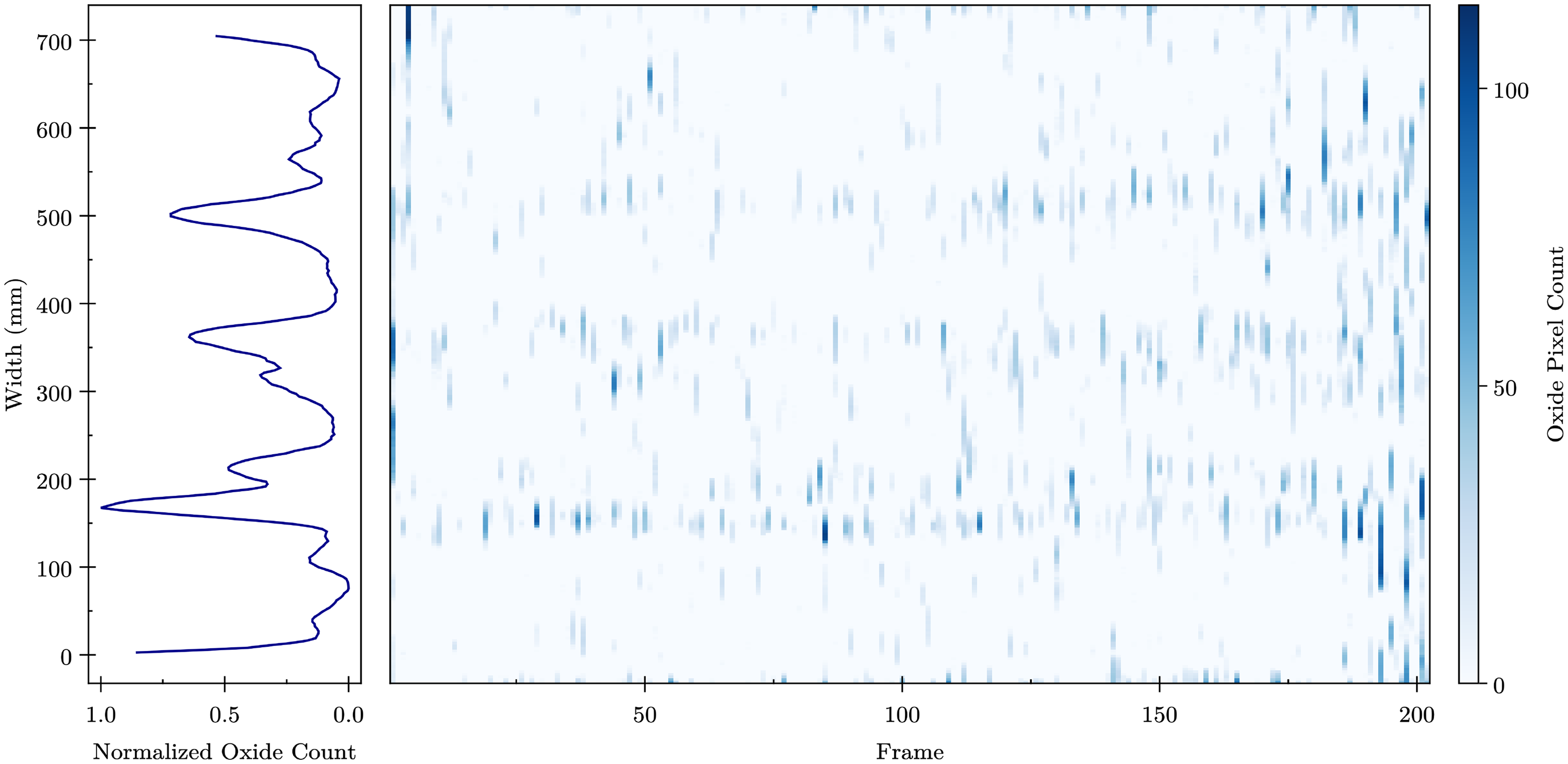
Positions of detected oxides for each frame of strip S15.

To quantify the seperation between regions of high oxide density, a 1D Gaussian kernel density estimator with a bandwidth value of 10 was applied to reduce background noise. Figure 12 presents the distribution of measured spacings across the minima from each plot. The spacings were found to have a median value of 59.4 mm and mean value of 64.5 mm.

Figure 12.

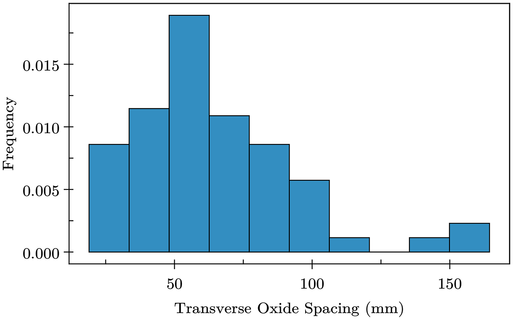
Histogram of measured spacings between minima from each strip.

When the spatial distribution between high oxide density regions is compared to the spray pattern of the descaler nozzles, there is agreement between the two measurements. Individual nozzles for descalers 1–6 can contribute 79, 81, 114, 152, 152, and 83 mm of descaling, respectively, and there is a total of 26 mm of over-overlap (13 mm on either side) with neighbouring nozzles. Figure 13 shows a simplified schematic diagram of the descaling region for three nozzles in descaler 6, with the oxide density profile for S9 overlaid.

Figure 13.

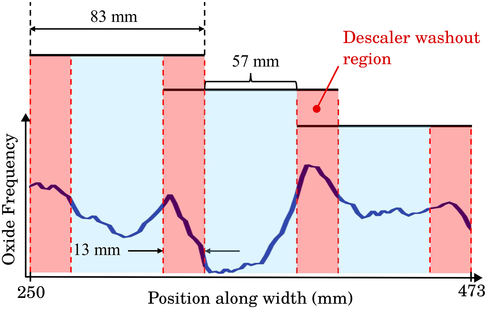
Rough rolling descaler schematic, with the oxide density plot of S9 overlaid. Red regions denote areas of descaler overlap that may cause washout.

If it is assumed that washout occurs in the overlap regions (reducing the descaling efficiency) and that the centre impact provides the most effective descaling, the expected distances between descaled regions for descalers 1–6 are approximately 53, 55, 88, 126, 126, and 57 mm, respectively. As shown in the overlaid oxide density profile in Figure 13, S9 demonstrates agreement with the descaler spacing values of 53, 55, and 57 mm, corresponding to descalers 1, 2, and 6. While S9 is a particularly strong example, this trend persists across most strips. Figure 12 shows the distribution of oxide peak spacings across all strips. The mode of this spacing distribution closely aligns with the 53 and 55 mm spacings of descalers 1 and 2.

Oxide location

To further investigate the influence of the descaling systems on the observed oxide density profiles, the locations of oxide peaks were analyzed. From the plots of Figures 10 and 11, it is evident that most strips exhibit a high density of oxides towards the mid-width.

Towards the outer regions (apart from strips 1, 3, 4, and 5) the presence of oxides was found to be minimal. This indicates that the nozzles positioned towards the edges of the strip provided better descaling than those at the centre. For the hot strip mill studied in this article, two different piping configurations are used: descalers 1, 3, 4, 5, and 6 are fed with a horizontal inlet, while descaler 2 is fed with a vertical inlet. Figure 14 provides a schematic diagram of descalers 2 and 4 to illustrate these differences.

Figure 14.

Vertical (a) and horizontal (b) feed descaler configurations.

The performance of descaling nozzles is correlated to the maximum impact force that it exerts on the strip surface. Maximum impact force can be calculated using equations (3) and 4, where $F_{T}$ is the total force, $ρ$ is the fluid density, $Q$ is the flow rate, $V$ is the velocity, $I_{m}$ is the impact force, $w$ is the spray width, and $t$ is the thickness of the spray pattern. To maintain adequate descaling, the turbulence and fluid velocities through the pipe need to be held at appropriate design levels. This can be done by controlling the pressure, flow rate, and header size.

F_{T} = ρ Q V

(3)

I_{m} = \frac{F_{T}}{w t}

(4)

For piping systems such as those used for descaling, the nozzles closest to the entrance of the pipe are most at risk of experiencing increased turbulence and approach velocities. As the approach velocity in the nozzles increases, the turbulence levels also increase, resulting in irregular spray patterns that reduce the impact force.³¹ Based on this, it is suggested that the high density of oxides detected towards the mid-width of the strip is the result of inadequate descaling from the center nozzles of the entry descaler of the roughing mill (descaler 2).

Oxide fraction

Figure 15 shows the total oxide fractions for S1–S15, determined using the model. As shown in the figure, there was a wide variation (0.5%–2.28%) between the strips, with S1 exhibiting the largest amount (2.28%). These differences in oxide fractions may be the result of a combination of both the Si content in the steel and the rough rolling of the slab. From Figure 15, the general trend of a decrease in oxide fraction was correlated with a decrease in Si content and roll reduction. This also suggests that the measured oxides are related to the primary scale formed in the reheat furnace.

Figure 15.

Total fraction of detected oxides for each strip. Fill colour and pattern indicate strip thickness.

Among the strips analysed, only S1 was expected to be influenced by Si. This is because even for Si-killed steels ( $\sim$ 0.25 wt-%), there is still enough Si to form Fe $_{2}$ SiO $_{4}$ during homogenisation in the reheat furnace.¹ Through the formation of Fe $_{2}$ SiO $_{4}$ , there is an associated increase in adhesion of FeO achieved through the formation of a FeO/Fe $_{2}$ SiO $_{4}$ eutectic compound.^13,32 This compound forms as a result of the temperatures reached in the reheat furnace. For S1, a homogenisation temperature of 1284 $\circ$ C was used, which makes the equilibrium state at the steel and scale interface FeO $+$ $L i q u i d$ .³² This liquid phase borders the FeO grains and penetrates the steel,³² and upon solidification, forms the FeO/Fe $_{2}$ SiO $_{4}$ eutectic.³² As a result of FeO being firmly bonded to the steel, descalers 1 and 2 may not fully remove it prior to entry into the roughing mill.^13,32 For strips S2–S15, the amount of Si is considerably lower than S1 (<0.06 wt-%), and the formation of Fe $_{2}$ SiO $_{4}$ is not expected.³³ This may explain why S1 (0.25 wt-% Si) had almost four times more surface oxides than S11–S14 (0.014 wt-% Si).

If the larger variations in oxide fraction are attributed to the Si content, the differences between the 10.97 and 11.51 mm strips may be due to the rough rolling process. These strips were rough rolled between 1097 $\circ$ C and 1284 $\circ$ C. At these temperatures, the oxides are expected to exhibit enhanced plasticity, allowing them to deform and get rolled into the strip.¹⁹ This leads to them elongating in the longitudinal direction, resulting in the morphology observed in Figure 9. Furthermore, under larger rolling reductions at elevated temperatures, the oxides become more compact, increasing their adhesion to the strip and reducing their likelihood of being descaled.¹⁹ Contrasting the 10.97 and 11.51 mm strips, the thinner strip endured a slightly larger degree of rolling deformation, and had slightly higher oxide fractions. Regarding S1, along with the influence of Si content, total roll reduction is also expected to influence the total oxide fraction. S1 was rolled between 1068 $\circ$ C and 1284 $\circ$ C, and the FeO/Fe $_{2}$ SiO $_{4}$ eutectic has been shown to deform when rolling close to its melting temperature (1205 $\circ$ C).³²

Novelty and limitations

Surface defect detection in TMCP is an area of active study. Contemporary methods often utilise a combination of feature extraction and image classification to flag areas of concern in grayscale images.^34,35 This approach typically utilises cameras that operate in visible-light wavebands (i.e. CCD³⁶). While these methods have demonstrated high classification accuracy, they are not able to utilise information about the temperature or emissivity of the surface. This limits their detection capabilities to defects that are visible to the human eye.

Local microstructural defects, (i.e. localised hard zones) are not always coupled with visible surface defects.³ If these local defects are caused by sufficiently thin oxide layers (on the order of 30 $μ m$ as suggested by Horsky et al.⁴), they may not be visible to human operators. By classifying on the basis of emissivity, the methodology presented in this work allows for an analysis of descaler performance without the need for costly ex-situ surface testing that would reveal thin oxide layers. Furthermore, the proposed method is non-parametric and, therefore, process agnostic; it does not require the operator to have knowledge of the emissivity of the surface oxides, as it utilises outlier detection rather than a mechanistic model.

The primary limitation of this non-parametric approach is the method used to estimate the true surface temperature (Figure 6). The assumption of constant temperature along the length of each IR frame only provides a first-order approximation. Figure 16 shows the expected error in predicted emissivity value as a function of error in true temperature. If the true difference in emissivity is on the order of 10%, there is only a $\sim \pm 15 \circ C$ margin of error on the estimate of the true temperature. Despite this limitation, the transverse oxide distributions predicted with the proposed methodology agree with descaler spacings. The morphology of the predicted oxides also agree with morphologies observed in the literature.¹

Figure 16.

Expected % error in predicted emissivity as a function of total error in prediction of true temperature. Calculated using average wavelength of 3.45 $μ m$ via Wien approximation.

Figure 17.

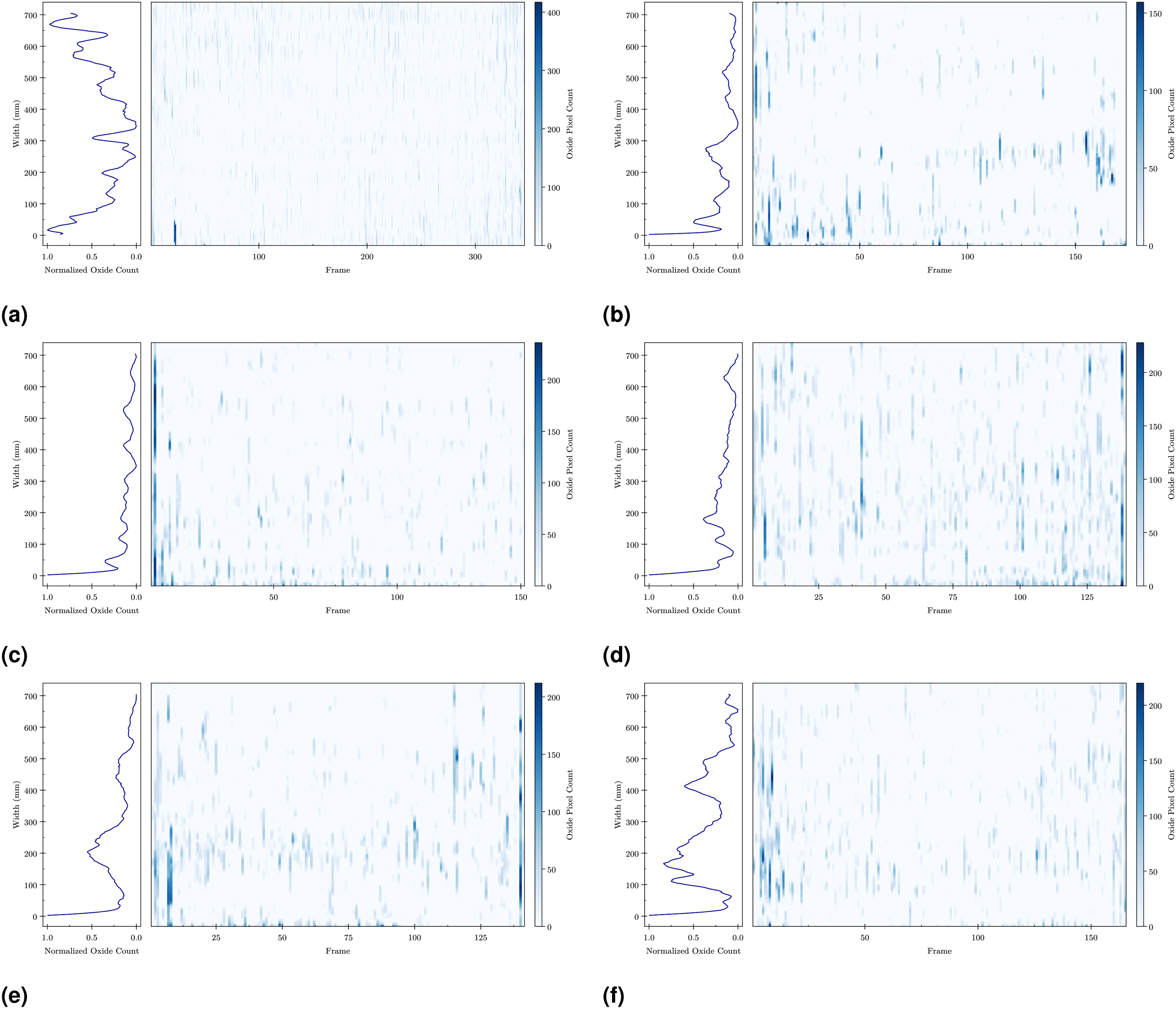
Positions of detected oxides in each frame along lengths of strips S1–S6.

Figure 18.

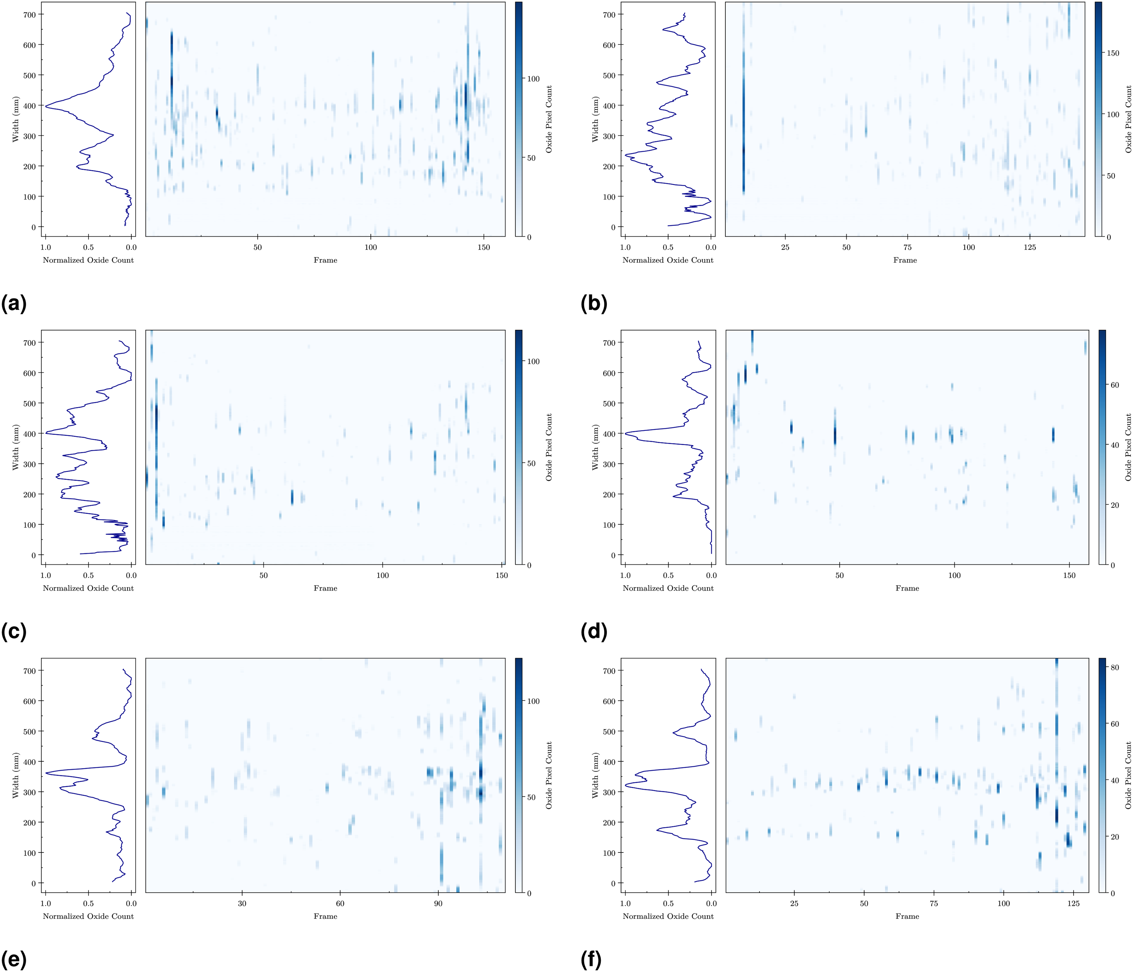
Positions of detected oxides in each frame along lengths of strips S7–S12.

Figure 19.

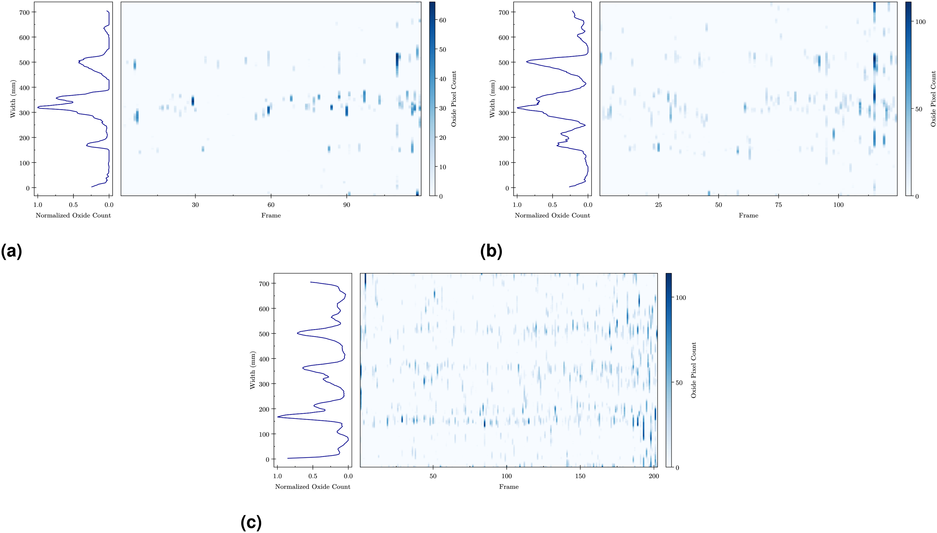
Positions of detected oxides in each frame along lengths of strips S13–S15.

Future work should investiage methods of measuring local emissivity directly, eliminating the need for true temperature predictions.

Conclusions

In-line assessment of descaler functionality was achieved through using IR video imaging in combination with a GP and GMM. The GP removed the influences of differential cooling on the strip, and allowed for the approximation of a true underlying temperature profile. With the true underlying profile, emissivty values could be calculated and clustered using the GMM. The oxide cluster was taken as the highest GMM component and used to identify oxides on the strip surface. Detected oxides had emissivty values ranging from 0.76 to 0.92, and morphologies resembling a smooth tear drop.

Oxide density plots were generated for each strip, and the corresponding spacings between minima were calculated to have a median and mean of 59.4 and 64.5 mm, respectively. The mean spacing value correlated strongly with the nozzle spacings of the reheat furnace (53 mm), roughing mill entry (55 mm), and finishing mill (57 mm) descalers. Furthermore, a large peak was present at the mid-width of most oxide density plots. This is suspected to be caused by the vertically fed descaler at the entry to the roughing mill.

A large variation in total oxide fractions (0.5%–2.28%) was measured among the strips, where the general trend of decreasing oxide fraction with decreasing Si and roll reduction was present. This trend is attributed to the increased adhesion of the oxide layer caused by the formation of Fe $_{2}$ SiO $_{4}$ , as well as oxides getting rolled into the strip.

Footnotes

Acknowledgements

The authors of this article would like to thank Stelco Inc. for allowing us to conduct plant trials on their TMCP line and their cooperation throughout the duration of this work. The financial support from Stelco Inc. and the Natural Sciences and Engineering Research Council of Canada (Grant CRDPJ 538420-18) is gratefully acknowledged.

ORCID iDs

Ry Karl

Jarrod Angove

Tihe Zhou

Funding

The authors disclosed receipt of the following financial support for the research, authorship and/or publication of this article: Funding for this work was provided by Stelco Inc. and the Natural Sciences and Engineering Research Council of Canada (Grant CRDPJ 538420-18).

Declaration of conflicting interests

The authors declared no potential conflicts of interest with respect to the research, authorship, and/or publication of this article.

Appendix A. Gaussian processes and mixture models

GP regression is a subset of a collection of machine learning models called kernel methods.³⁷ These methods work on the principle of predicting functions directly, rather than a parameterised approximation. GPs apply some statistical methods to these algorithms to create more robust predictions. The following section explains how these models work and some of the considerations that are made when constructing them. Most of the notation is taken from Murphy,³⁷ with additional insights from Rasmussen.³⁸ The reader is encouraged to see these texts for a more comprehensive overview of GP regression.

Every dataset has input points and response points. The input points can be thought of as a vector, where every entry is the value of the control variable for a given observation. If there are multiple control variables, each entry is itself a vector with length $d$ . The response points are then a vector of the responding variable for each corresponding observation. For the scope of this work, only scalar-valued responses will be considered. This can be written as follows:

X = [\begin{matrix} [x_{1, a}, x_{1, b}, \dots, x_{1, d}] \\ ⋮ \\ [x_{n, a}, x_{n, b}, \dots, x_{n, d}] \end{matrix}] = [\begin{matrix} x_{1} \\ ⋮ \\ x_{n} \end{matrix}], y = [\begin{matrix} y_{1} \\ ⋮ \\ y_{n} \end{matrix}]

The fundamental idea behind GP models is that two points with similar inputs should have similar response values. This assumption is encoded in the form of a covariance matrix

K

K

contains the covariance for every pair of points in

X

. This covariance is approximated by a kernel function

k

, which maps the distance between two points in the input space to a covariance value. This can be denoted as follows:

K = {k (x, x^{'}) | x \in X, x^{'} \in X} = k (X \times X) = [\begin{matrix} k (x_{1}, x_{1}) & \dots & k (x_{1}, x_{n}) \\ ⋮ & ⋱ & ⋮ \\ k (x_{n}, x_{1}) & \dots & k (x_{n}, x_{n}) \end{matrix}]

where (

\times

) denotes the Cartesian product. If two points have similar values in input space, their distance will be small and the kernel function will return a large covariance. The kernel function can take many forms, but this concept holds true for all of them. One example of a kernel function is the squared exponential kernel, shown in the following equation: (5)

k (x, x^{'}) = σ^{2} \exp (- \frac{(x - x^{'})^{2}}{2 l^{2}})

This kernel has two hyperparameters:

l

, often referred to as the lengthscale, and

σ

, which is a scaling parameter. The parameters can be adjusted to improve the fit of the model with the data. These are the only parameters in the model. This is one aspect of why GPs are so powerful: the vast majority of the prediction comes from the data, not the model.

To make predictions, it is first assumed that every data point is sampled from an $n$ -dimensional Gaussian distribution with covariance $K$ .

y \sim N (μ, K)

The marginal likelihood of the response with respect to the input can then be calculated as a function of the kernel parameter(s)

θ

\log p (y | X, θ) = - \frac{1}{2} y K^{- 1} y^{⊤} - \frac{1}{2} \log | K | - \frac{n}{2} \log (2 π)

where

n

is the number of points in the dataset. This can be optimised with most gradient descent algorithms. Once the kernel parameters are optimised, inference is run by creating a joint distribution between the observed response (

y (X)

) and the response at some unknown point (

f_{⋆} (X_{⋆})

): (6)

{\hat{K}}_{X, X} ≜ k (X \times X) + σ_{N}^{2} I K_{X, ⋆} ≜ k (X \times X_{⋆}) K_{⋆, ⋆} ≜ k (X_{⋆} \times X_{⋆})

(7)

(\begin{matrix} y \\ f_{⋆} \end{matrix}) = N ((\begin{matrix} μ \\ μ_{⋆} \end{matrix}), (\begin{matrix} {\hat{K}}_{X, X} & K_{X, ⋆} \\ K_{⋆, X} & K_{⋆, ⋆} \end{matrix}))

where

I

is an

n

n

identity matrix and

σ_{N}

can be interpreted as the noise of the response signal. The mean and variance of the predicted response can then be calculated as follows: (8)

μ_{⋆ | X} = μ_{⋆} + K_{⋆, X} {\hat{K}}_{X, X}^{- 1} (y - μ)

(9)

Σ_{⋆ | X} = K_{⋆, ⋆} - K_{⋆, X} {\hat{K}}_{X, X}^{- 1} K_{X, ⋆}

GP regression is most commonly used for time-series modelling³⁹ and the analysis of geospatial data.⁴⁰ More recently, GP regression has been applied to the analysis of IR images in the fields of food science,⁴¹ forestry,⁴² and astronomy.⁴³ In the field of physical metallurgy, GP regression has been used to forecast temperatures of molten steel in a ladle furnace,⁴⁴ predict austenite start temperatures,⁴⁵ and predict oxygen consumption in a converter steelmaking process.⁴⁶ In this work, GP regression is utilised in a similar fashion to signal denoising, which has been demonstrated extensively in the literature.^47–50

A GMM is a probabilistic model that is used to deconvolute an overall distribution into several sub-populations that exist within it. In this model, the assumption that every data point belongs to a specific component is made. Equation (10) illustrates this relationship, where $k$ is the individual Gaussian and $K$ is the number of components. Each of these components is described by with a mean, variance, and weight. (10)

k \in {1, \dots, K}

The probability density function of the GMM is then a weighted sum of the

K

Gaussian distributions. This is represented by equation (11) where for the

i

th component

π

is the weighting and

N

is the normal distribution. (11)

p (x | θ) = \sum_{i}^{K} π_{i} N (x | μ_{i}, σ_{i}^{2})

To determine the optimum parameters for the GMM model, an iterative algorithm called expectation–maximisation (EM) is used. EM essentially calculates the posterior probability that value

x_{i}

belongs to component

k_{i}

given the current set of parameters

N (x_{i} | μ_{k}, Σ_{k})

. Equation (12) shows the calculation for the expectation step of data point

i

in component

k

where

Σ_{k}

is the covariance matrix of component

k

. (12)

γ_{i k} = \frac{π_{k} N (x_{i} | μ_{k}, Σ_{k})}{Σ_{j = 1}^{K} π_{j} N (x_{i} | μ_{j}, Σ_{j})}

Given the value from equation (12), the values of

μ_{k}

Σ_{k}

, and

π_{k}

are updated to maximise the expected log-likelihood; equations (13) to (15). After each update, the convergence is checked by calculating the new log-likelihood with equation (16). (13)

μ_{k} = \frac{Σ_{i = 1}^{N} γ_{i k} x_{i}}{Σ_{i = 1}^{N} γ_{i k}}

(14)

Σ_{k} = \frac{Σ_{i = 1}^{N} γ_{i k} (x_{i} - μ_{k}) (x_{i} - μ_{k})^{⊤}}{Σ_{i = 1}^{N} γ_{i k}}

(15)

π_{k} = \frac{1}{N} \sum_{i = 1}^{N} γ_{i k}

(16)

\log L (θ | X) = \sum_{i = 1}^{N} \log (\sum_{k = 1}^{K} π_{k} N (x_{i} | μ_{k}, Σ_{k}))

Appendix B. Oxide denisty plots

References

Ginzburg

. Steel-rolling technology: theory and practice. CRC Press, 1989.

Jang

Lee

Kim

et al. Investigation of the slab heating characteristics in a reheating furnace with the formation and growth of scale on the slab surface. Int J Heat Mass Transfer 2010; 53: 4326–4332.

Fairchild

Newbury

Anderson

et al. Local hard zones in sour service steels. In: Volume 4: Materials technology. Glasgow, Scotland, UK: American Society of Mechanical Engineers, p.10. Available at: https://asmedigitalcollection.asme.org/OMAE/proceedings/OMAE2019/58790/Glasgow,%20Scotland,%20UK/1067694.

Horsky

Hrabovsky

Raudensky

. Impact of the oxide scale on spray cooling intensity. In: International Conference on Heat Transfer, Fluid Mechanics and Thermodynamics, 2014, pp.6. University of Pretoria. Available from: http://hdl.handle.net/2263/44729.

Tsukamoto

Kita

Inoue

et al. On the onset of quench during spray cooling: the significance of oxide layers. Appl Therm Eng 2020; 179: 115682. DOI: 10.1016/j.applthermaleng.2020.115682.

Chabičovský

Hnízdil

Tseng

et al. Effects of oxide layer on Leidenfrost temperature during spray cooling of steel at high temperatures. Int J Heat Mass Transfer 2015; 88: 236–246. DOI: 10.1016/j.ijheatmasstransfer.2015.04.067.

Smith

Spinelli

. Surface hard zone phenomenon in TMCP line pipes for sour service: A state of the art review. In: CORROSION 2021, 2021. OnePetro. Available from: https://onepetro.org/NACECORR/proceedings-abstract/CORR21/CORR21/D021S006R009/463882.

Jiang

Zhao

et al. A review of microstructure and microtexture of tertiary oxide scale in a hot strip mill. Key Eng Mater 2016; 716: 843–855.

Graf

Kawalla

. Scale development on steel during hot strip rolling. La Metall Ital 2014: 43–49. Available from: https://www.fracturae.com/index.php/aim/article/view/1227.

10.

Chen

Yuen

WYD

. Examination of oxide scales of hot rolled steel products. ISIJ Int 2005; 45: 52–59.

11.

Sun

Tieu

Jiang

et al. Surface characteristics of oxide scale in hot strip rolling. J Mater Process Technol 2003; 140: 76–83.

12.

Krzyzanowski

Beynon

. Modelling the behaviour of oxide scale in hot rolling. ISIJ Int 2006; 46: 1533–1547.

13.

Song

Suh

Bhadeshia

HKDH

. Oxidation of silicon containing steel. Ironmak Steelmak 2012; 39: 599–604.

14.

Nasr

Yule

Bendig

et al. Spraying hot surfaces for making steel and other metals. In: Industrial Sprays and Atomization: Design, Analysis and Applications. Springer, 2002, pp.379–440.

15.

PODRO PIP

MEDIJ

. Overcooling in overlap areas during hydraulic descaling. Mater Tehnol 2016; 50: 575–578.

16.

Farrugia

Richardson

Lan

. Advancement in understanding of descalability during high pressure descaling. In: Key engineering materials. Vol. 622. Trans Tech publications, pp.29–36.

17.

Krzyzanowski

Beynon

. Effect of oxide scale failure in hot steel rolling on subsequent hydraulic descaling: Numerical simulation. In: Proceedings of the 3rd international conference on hydraulic descaling, London, United Kingdom. pp.14–15.

18.

Nakamura

Sato

. Descalability on reheated steel slabs at high temperature. Tetsu-to-Hagané 1994; 80: 237–242.

19.

Han

Zhou

Wang

et al. Effect of rolling reduction and temperature on the oxide scale of hot rolled mild steel strip. Mater Res 2019; 22: 1–7. Available from: https://www.scielo.br/j/mr/a/9ZMhCrBqSvn7nvgqpZFjh7L/?lang=en.

20.

Guedia Guemo

Prodanovic

Militzer

. Simulation of runout table cooling. Steel Res Int 2019; 90: 1800361.

21.

Jayaraman

. Machine learning for analyses and automation of structural characterization of polymer materials. Prog Polym Sci 2024; 101828.

22.

Jasti

VDP

Zamani

Arumugam

et al. Computational technique based on machine learning and image processing for medical image analysis of breast cancer diagnosis. Secur Commun Netw 2022; 2022: 1918379.

23.

Bürger

Buck

Pauli

et al. Image-based object classification of defects in steel using data-driven machine learning optimization. In: 2014 International conference on computer vision theory and applications (VISAPP). Vol. 2. IEEE, pp.143–152.

24.

Lugin

Müller

Finckbohner

et al. Automated surface defect detection in forged parts by inductively excited thermography and magnetic particle inspection. Quant Infr Therm J 2023; 1–3.

25.

Kim

Park

Jang

et al. Automated classification of thermal defects in the building envelope using thermal and visible images. Quant Infr Therm J 2023; 20: 106–122.

26.

Helvig

Trouvé-Peloux

Gaverina

et al. Automated crack detection on metallic materials with flying-spot thermography using deep learning and progressive training. Quant Infr Therm J 2023; 1–20.

27.

Karl

. Integrated computational modeling of run-out table ohase transformations. PhD Thesis, University of Alberta, 2023.

28.

del Campo

Pérez-Sáez

Tello

. Iron oxidation kinetics study by using infrared spectral emissivity measurements below 570

\circ

C. Corros Sci 2008; 50: 194–199. DOI: 10.1016/j.corsci.2007.05.029.

29.

Chen

Bao

et al. A study on the heat transfer characteristics of steel plate in the matrix laminar cooling process. Materials 2021; 14: 5680. DOI: 10.3390/ma14195680.

30.

Wang

. The study of improving the strip flatness in run-out-table during laminar cooling. Int J Adv Manuf Technol 2018; 95: 4419–4437. DOI: 10.1007/s00170-017-1558-5.

31.

Peterson. Maximizing impact force from descale headers using CFD analysis. London, UK: The Institute of Materials, Minerals and Mining IOM3; 2018. p. 27–34. Available from: https://www.open-access.bcu.ac.uk/7204/7/OXI%20Abstracts.pdf

32.

Fukagawa

Okada

Maehara

. Mechanism of red scale defect formation in Si-added hot-rolled steel sheets. ISIJ Int 1994; 34: 906–911.

33.

Suarez

Schneider

Houbaert

. Effect of Si on high-temperature oxidation of steel during hot rolling. In: Defect and diffusion forum. Vol. 273. Trans Tech Publication, pp.655–660.

34.

Song

Meng

et al. An end-to-end steel surface defect detection approach via fusing multiple hierarchical features. IEEE Trans Instrum Meas 2020; 69: 1493–1504. DOI: 10.1109/TIM.2019.2915404.

35.

et al. Multi-scale sensing and multi-dimensional feature enhancement for surface defect detection of hot-rolled steel strip. Nondestruct Test Eval 2025; 40: 3669–3692. DOI: 10.1080/10589759.2024.2408441.

36.

Song

Yan

. A noise robust method based on completed local binary patterns for hot-rolled steel strip surface defects. Appl Surf Sci 2013; 285: 858–864. DOI: 10.1016/j.apsusc.2013.09.002.

37.

Murphy

. Probabilistic ,achine learning: an introduction. Adaptive Computation and Machine Learning Series. Cambridge, Massachusetts: The MIT Press, 2022.

38.

Rasmussen

Williams

CKI

. Gaussian processes for machine learning. Adaptive Computation and Machine Learning. Cambridge, Mass: MIT Press, 2006.

39.

Roberts

Osborne

Ebden

et al. Gaussian processes for time-series modelling. Phil Trans R Soc A 2013; 371: 20110550. DOI: 10.1098/rsta.2011.0550.

40.

Murakami

Yamagata

Hirano

. Chapter Four - Geostatistics and Gaussian process models. In: Yamagata Y and Seya H (eds) Spatial analysis using big data. Academic Press, 2020, pp.57–112. Available at: https://www.sciencedirect.com/science/article/pii/B9780128131275000047.

41.

Arefi

Sturm

von Gersdorff

et al. Vis-NIR hyperspectral imaging along with Gaussian process regression to monitor quality attributes of apple slices during drying. LWT 2021; 152: 112297. DOI: 10.1016/j.lwt.2021.112297.

42.

Hultquist

Chen

Zhao

. A comparison of Gaussian process regression, random forests and support vector regression for burn severity assessment in diseased forests. Remote Sens Lett 2014; 5: 723–732. DOI: 10.1080/2150704X.2014.963733

43.

Muyskens

Goumiri

Priest

et al. Star–galaxy image separation with computationally efficient Gaussian process classification. Astron J 2022; 163: 148. DOI: 10.3847/1538-3881/ac4e93.

44.

Wang

Qiao

et al. Dynamic selective Gaussian process regression for forecasting temperature of molten steel in ladle furnace. Eng Appl Artif Intell 2022; 112: 104892. DOI: 10.1016/j.engappai.2022.104892.

45.

Bailer-Jones

CAL

Bhadeshia

HKDH

MacKay

DJC

. Gaussian process modelling of austenite formation in steel. Mater Sci Technol 1999; 15: 287–294. DOI: 10.1179/026708399101505851.

46.

Jiang

Shen

Zheng

. Gaussian process-based hybrid model for predicting oxygen consumption in the converter steelmaking process. Processes 2019; 7: 352. DOI: 10.3390/pr7060352.

47.

Zhu

Carpenter

Gonzalez

et al. Computed tomography perfusion imaging denoising using Gaussian process regression. Phys Med Biol 2012; 57: N183. DOI: 10.1088/0031-9155/57/12/N183.

48.

Hua

Dai

et al. Image denoising via neighborhood-based multidimensional Gaussian process regression. Signal Image Video Process 2023; 17: 389–397. DOI: 10.1007/s11760-022-02245-9.

49.

Bai

Peng

. Radar image series denoising of space targets based on Gaussian process regression. IEEE Trans Geosci Remote Sens 2019; 57: 4659–4669. DOI: 10.1109/TGRS.2019.2892183.

50.

Gilboa

Cunningham

Nehorai

et al. Image interpolation and denoising for division of focal plane sensors using Gaussian processes. Opt Exp 2014; 22: 15277–15291. DOI: 10.1364/OE.22.015277.