Sage Journals: Discover world-class research

Abstract

This study explored the effect of varying steel skelp temperature (500 °C–600 °C) on the subsequent temperature-time (T-t) profile during and after coiling of low C (0.05 wt. %) X70 microalloyed steels. Three industrially produced steel coils with similar rough rolling temperatures (∼1050 °C) and finish rolling temperatures (∼850 °C) but different coiling temperatures (500 °C–600 °C) and different skelp thicknesses (19 mm and 25 mm) were studied. The surface temperature of each coil was measured using an infrared video camera. A three-dimensional heat transfer model was developed to predict the T-t profiles. A lower (∼60 °C) initial skelp temperature near the head and tail of the skelp led to a reduced coil temperature. A higher (∼50 °C) temperature near the head and tail region of the skelp resulted in a more uniform coil temperature (a difference of ∼10 °C instead of ∼50 °C).

Keywords

Coil cooling infrared measurement ABAQUS thermal model X70 coiling FEM

Introduction

Achieving homogenous mechanical properties along the length of a steel skelp produced through thermo-mechanical controlled processing (TMCP) is important for steel manufacturers. In TMCP, the final processing step is to coil the steel skelp after laminar cooling on the run-out table (ROT). For skelp produced as hot rolled coil, variations of temperature during and after laminar cooling leads to variations in the steel temperature during coiling and can influence the final microstructure and mechanical properties of microalloyed X70 steels.^1–5 Specifically, the steel temperature during the early stage (∼1 h) of coil cooling can have a significant impact on the size of the nano-carbides formed.^3–5 For microalloyed steels, it has been shown that a change in the initial skelp temperature from 660 °C to 540 °C resulted in a decrease in the average size of the nano-carbides from 7.1 nm to 3.1 nm.⁵ Accompanying this decrease in carbide size, there was an increase in yield strength (estimated using Ashby–Orowan equation) of 81.2 MPa. Therefore, an understanding of the temperature–time profile at any location in the coil and its effect on precipitation and mechanical properties is important.

The cooling of a steel coil is a function of many variables, including initial skelp temperature, skelp thickness and the effective heat transfer conditions to which the coil is subjected.^6–9 Previous studies have measured coil temperatures using direct contact thermocouples^7–9 or infrared (IR) imaging.^10,11 An important parameter for infrared measurements is the emissivity of the steel at different temperatures. The emissivity of steel is a function of composition, temperature, surface finish and viewing angle,^10–13 with temperature having a significantly stronger impact. Liu et al.¹⁰ studied the temperature of three different steels in the temperature range of 477–877 °C. The emissivity of the steels was found to vary between 0.5 and 0.77, following a typical S curve with lower emissivity at lower temperatures. A number of finite element thermal models of coil cooling have been developed^6–11 to predict the temperature in a steel coil, including the effect of initial skelp temperature, skelp thickness and boundary conditions. Karlberg^8,9 modelled the cooling of steel coils with different skelp thicknesses (between 1 mm and 17 mm) and coiling temperatures (between 600 °C and 700 °C) using an equivalent thermal conductivity approach for a reduced two-dimensional coil geometry. The difference in temperature observed for steel coils (with skelp thickness of 6 mm and 17 mm) as a function of time at different locations was small (<10 °C). More recent studies^10,11 have shown that there is a large difference in temperature (∼80–100 °C) between the surface and central regions of steel coils and that a three-dimensional model of the steel coil is deemed necessary. Patrault et al.¹⁰ showed that the nature of cooling experienced by different regions of the coil varies significantly. For instance, the inner surface region of the coil shows an increase in temperature after the coil is removed from the mandrel. Unfortunately, the available studies assume a single constant value of skelp temperature as an initial condition in their models. The influence of non-uniform skelp temperature on subsequent coil cooling has not been studied.

In this study, an IR video camera placed in close proximity (∼5 m) to the coiling system was used to measure coil surface temperature as a function of time. Additionally, the temperature of the steel skelps as a function of skelp length prior to coiling was measured using a pyrometer. A three-dimensional finite element thermal model was developed and validated using the IR temperature measurements. To determine the effective heat transfer coefficients for the thermal model, the temperature of the coil as a function of time and location was used. The non-uniform skelp temperature prior to coiling was accounted for in the thermal model by using it as the initial coil temperature. The model predictions were used to assess the effect of the initial skelp temperature and boundary conditions on overall coil cooling. In addition, an idealised skelp temperature profile (∼50 °C higher head and tail temperatures) was developed to provide more uniform cooling of the coil.

Materials and experimental procedure

Materials

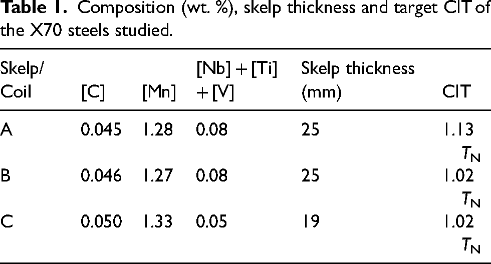
Three as-cast steel ingots (labelled A, B and C) of microalloyed X70 steel were thermo-mechanically controlled and processed (TMCP) into skelp of 19 mm or 25 mm thickness. The steel ingots were homogenised at 1250 °C for ∼2 h, followed by rough rolling at ∼1050 °C and finish rolling at ∼850 °C. After rolling, the skelps were cooled to a specific coiling interrupt temperature (CIT) and then coiled. The CIT values are provided as normalised temperatures (T_N) for proprietary reasons. The details of the three steels along with their compositions (in wt.%) are shown in Table 1. Steels A and B had a skelp thickness of 25 mm, while steel C had a skelp thickness of 19 mm. The CIT for steel A was higher (1.13 T_N) compared with steels B and C (1.02 T_N). The nominal carbon composition for all steels was similar (∼0.05 wt.%) and the nominal Nb + Ti + V composition for steels A and B (0.08 wt.%) was higher than that for steel C (0.05 wt.%).

Table 1.

Composition (wt. %), skelp thickness and target CIT of the X70 steels studied.

Skelp/Coil	[C]	[Mn]	[Nb] + [Ti] + [V]	Skelp thickness (mm)	CIT
A	0.045	1.28	0.08	25	1.13 T_N
B	0.046	1.27	0.08	25	1.02 T_N
C	0.050	1.33	0.05	19	1.02 T_N

Experimental procedure

Pyrometer temperature measurement

The skelp temperatures prior to coiling for all three steels were measured using a process pyrometer (positioned ∼10 m away from the steel skelps). The variation in temperature along the normalised skelp length (x_N) for skelp A (taken upstream of the coiler) is shown in Figure 1. This variation is considered during the modelling of the cooling of each coil.

Figure 1.

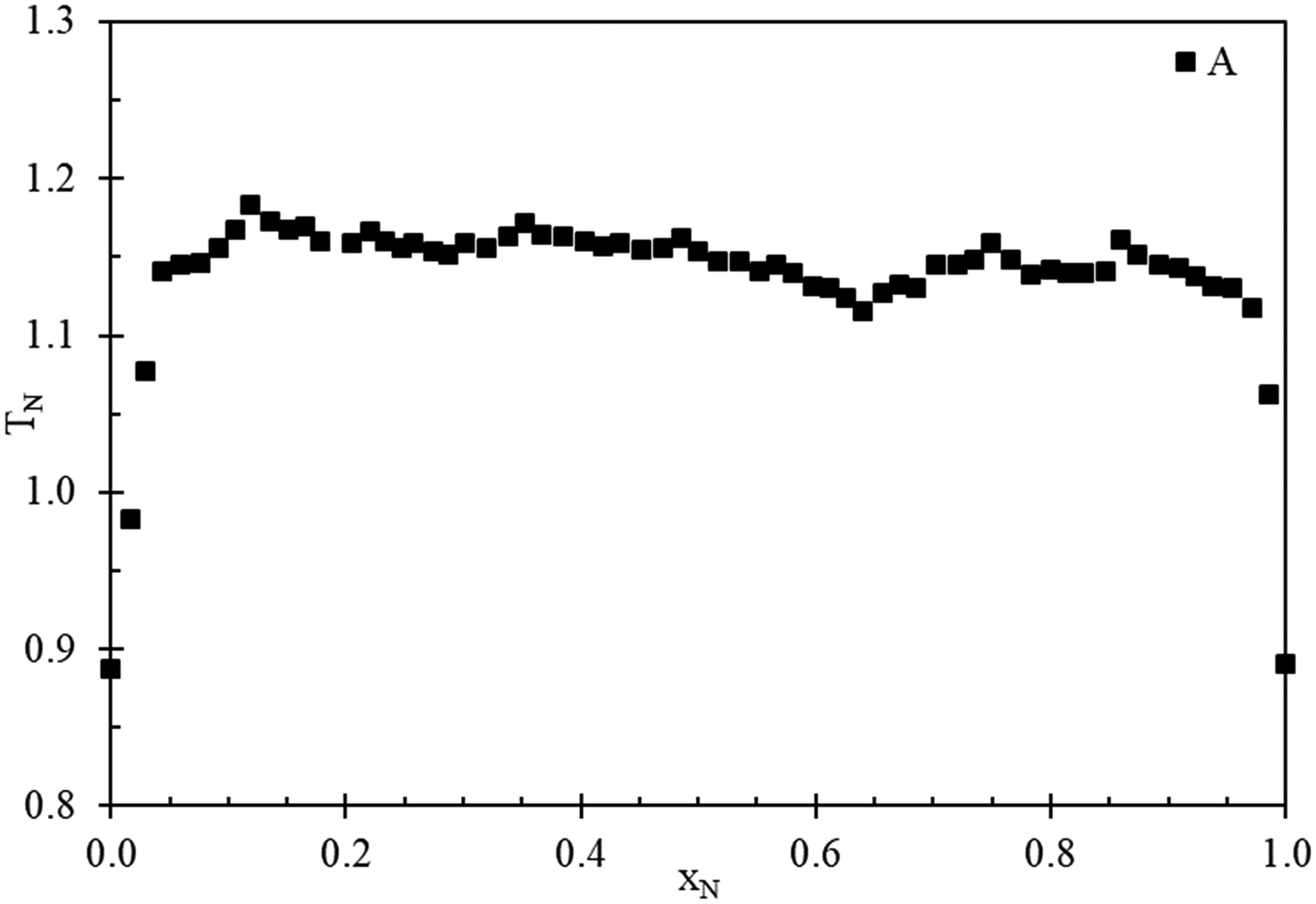
Measured normalized skelp temperature (T_N) for skelp A as a function of normalised skelp length (x_N).

IR camera measurements

The surface temperature of the coils was measured using a TELOPS IR camera (detection band of 3 to 5 μm) by positioning the camera ∼5 m away from the steel coils. The IR temperature image taken for coil A at ∼12 min from the start of coiling (i.e., wrapping of skelp around the mandrel) is shown in Figure 2. The bright regions (white) in Figure 3 correspond to relatively high temperatures, while the red regions indicate lower temperatures. In general, the middle radius location of the coil is hotter than the locations near the inner and outer radii. The blue colour (very low temperatures) around the outer diameter of the coil is assumed to be a temperature artefact associated with the coil edge. The dashed black line corresponds to the location (on the coil flat surface) at which temperature line scans across the coil radius were measured.

Figure 2.

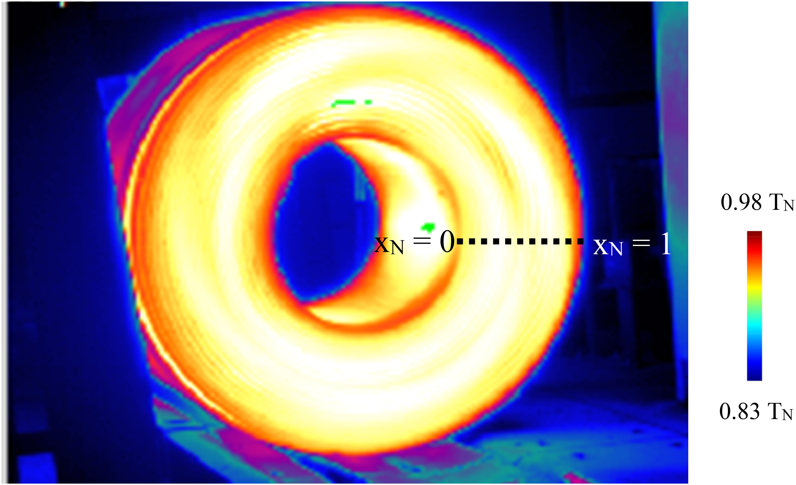
IR camera image taken for coil A at ∼12 min from the start of coiling.

Figure 3.

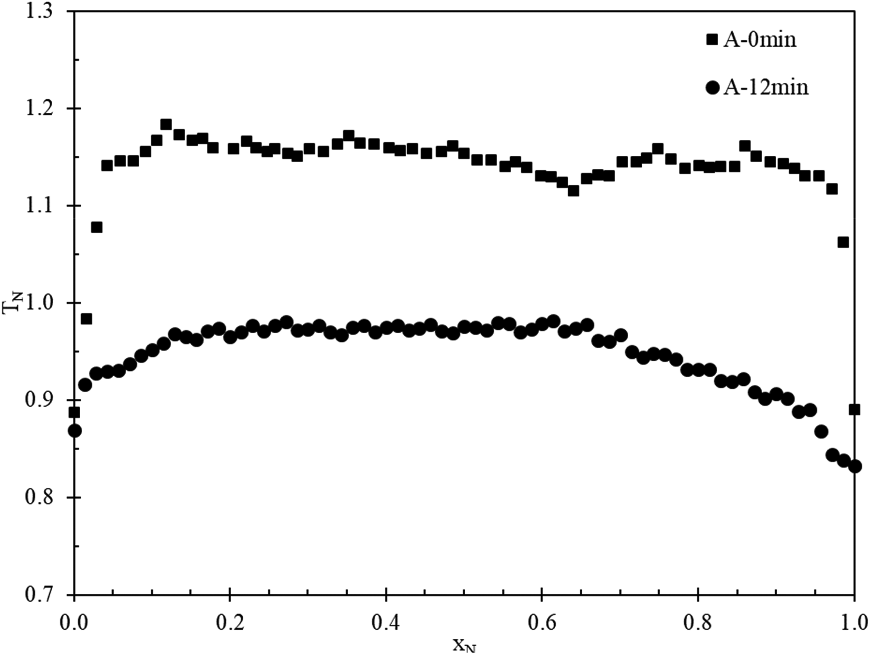
Measured T_N for coil A at 0 min and 12 min taken along the dashed line in Figure 2.

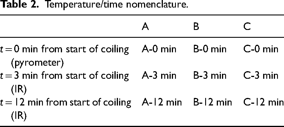
Figure 3 shows the normalised temperature profiles measured by the IR camera for coil A at a position on the coil corresponding to the dashed line shown in Figure 2. The radial position of each temperature measurement along the dashed line is converted to the normalised skelp length. The emissivity used for the temperature measurements of coil A was 0.62 and was determined by correlating specific coil temperatures with the measured skelp pyrometer data. Included in Figure 3 is the normalised temperature measurement of skelp A just before coiling (denoted by A-0 min). The temperature profile of the coil after 12 min from the start of coiling (denoted by A-12 min) is significantly less than the measured skelp temperature profile and is attributed to the extent of cooling that has taken place. Table 2 shows a list of nomenclature used for each coil.

Table 2.

Temperature/time nomenclature.

	A	B	C
t = 0 min from start of coiling (pyrometer)	A-0 min	B-0 min	C-0 min
t = 3 min from start of coiling (IR)	A-3 min	B-3 min	C-3 min
t = 12 min from start of coiling (IR)	A-12 min	B-12 min	C-12 min

Thermal modelling of the coil system

Finite element thermal model development

The full 3D finite element (FE) discretisation of the entire coil system is shown in Figure 4. Both the coil (dark green colour) and the mandrel (light brown colour) are included in the thermal model. The heat transfer conditions include conduction between the mandrel and the inner circumference of the coil (perfect contact is assumed) and both convection and radiation for all other coil surfaces. Perfect contact between the individual layers of steel in the coil was assumed. The temperature across the thickness and width of the skelp was assumed to be constant and equal to the value measured by the pyrometer at the corresponding location. The coils in this work experienced non-uniform cooling for different surfaces. Additionally, the width of the coils, i.e., the length of the cylinder (∼1.2 m) was comparable to the outer radius of the coils (∼1 m). Therefore, a 3D model was deemed necessary.

Figure 4.

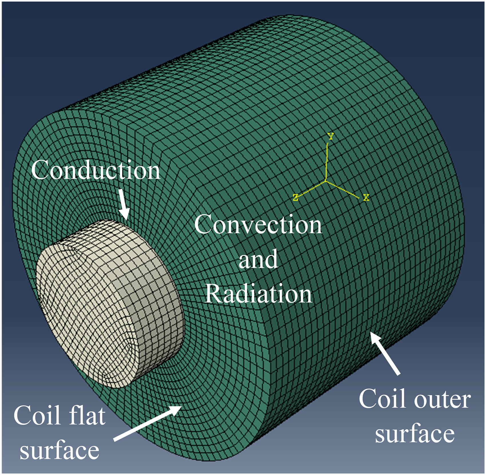
Coil and mandrel finite element mesh and boundary conditions.

The cooling process of a typical coil is as follows. First, the strip is coiled on the mandrel while it is exposed to air. Once the coiling process is complete, the surface of the coil is cooled by external enhanced cooling for a predetermined time period. The enhanced cooling is terminated and the coil is removed from the mandrel and transported to a mill yard for further cooling. For thermal modelling, these cooling process steps can be divided into four stages of coiling denoted by S1, S2, S3 and S4.

S1 – coil cooling is by conduction with the mandrel and convection and radiation from the outer coil surfaces.

S2 – coil cooling is by conduction with the mandrel and enhanced convection from the outer coil surfaces.

S3 – coil cooling is by conduction with the mandrel and convection and radiation from the outer coil surfaces.

S4 – coil cooling is by convection and radiation from all coil surfaces including the inner coil surface (occupied by the mandrel during S1, S2 and S3).

The convection cooling term h₁ (in S1, S3 and S4) is relatively low (25 W/m²K) and is consistent with natural convection (air cooling).¹⁴ The enhanced cooling terms h₂ and h₃ in S2 are 1000 W/m² K and 400 W/m² K, respectively, and correspond to the enhanced cooling applied during S2 and are consistent with forced convection.^15,16

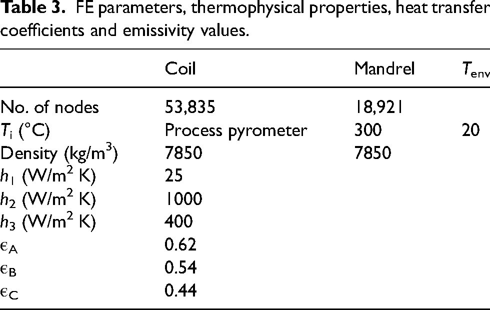
Table 3 details the thermophysical properties of both the mandrel and the coil and summarises the convective heat transfer coefficient and radiation emissivity values used. The heat capacity and thermal conductivity (C_p and k, respectively) were taken to be temperature dependent.⁶ The radiation emissivities (ε_A, ε_B and ε_C) are the calibrated values obtained for coils A, B and C, respectively. The decrease in emissivities (ε_A, ε_B and ε_C) with decreasing T_i is consistent with measured values reported in the literature.^12,13,17,18 The initial coil temperature (T_i) is the measured process pyrometer temperature along the length of the skelp immediately before coiling. The environment temperature (T_env) was taken as 20 °C.

Table 3.

FE parameters, thermophysical properties, heat transfer coefficients and emissivity values.

	Coil	Mandrel	T _env
No. of nodes	53,835	18,921
T_i (°C)	Process pyrometer	300	20
Density (kg/m³)	7850	7850
h₁ (W/m² K)	25
h₂ (W/m² K)	1000
h₃ (W/m² K)	400
ε_A	0.62
ε_B	0.54
ε_C	0.44

A series of model tests were carried out to determine the mesh size and time step required to obtain a stable and converging result. Some of the various test results are shown in the Appendix. It was determined that a mesh size of 0.04 m provided a stable and converging solution.

Initial coil temperature

Figure 5 shows the initial temperature profile for coil A that was used in the model. The measured temperature at the head of the skelp (x_N= 0) is assumed to be the temperature at the inner surface of the coil. The measured temperature at the tail of the skelp (x_N= 1) is assumed to be the temperature at the outer surface of the coil. The temperature variation along the radius of the coil corresponds to the temperature variation along the length of the skelp.

Figure 5.

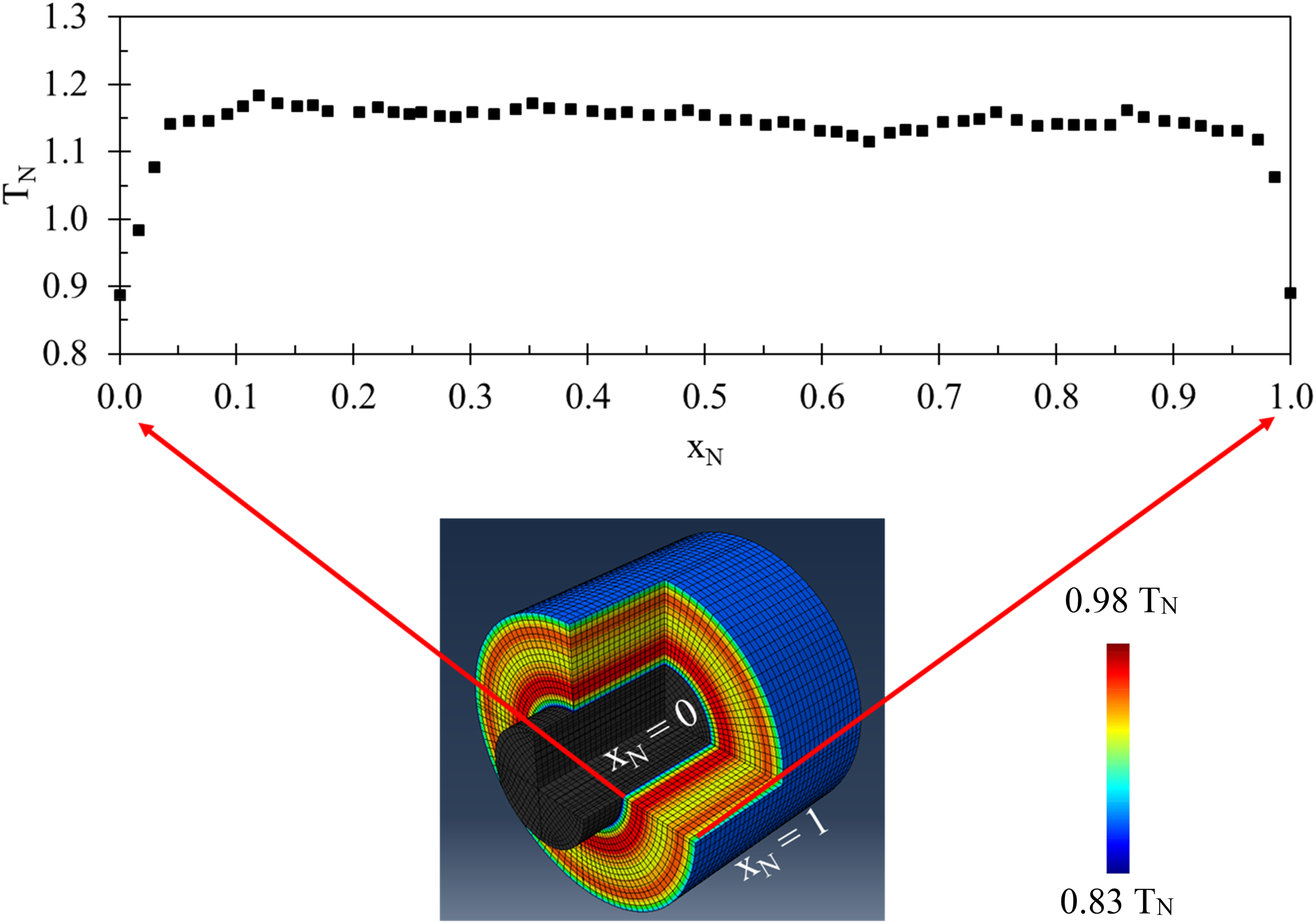
Initial temperature distribution for thermal simulation of coil A.

Results and discussion

IR measurements

Figure 6 shows the measured IR temperature distribution across the flat surface of coil A at ∼3 min from the start of coiling (denoted by A-3 min). The temperatures near the outer surface (x_N= 1) and inner surface (x_N= 0) are lower due to enhanced cooling on the outer surface and conduction cooling with the mandrel at the inner surface, respectively. The local temperature fluctuations (e.g. between points a and b in Figure 6) are attributed to the interfaces between the individual coil layers and are less than 10 °C. The effect of heat transfer between the individual coil layers and its effect on coil cooling was modeled^7,8 for skelp thicknesses between 1.7 mm and 6 mm. The predicted coil temperatures for each skelp thickness were similar (difference of less than 10 °C), indicating that the effect of interfacial layer heat transfer was not significant. For the skelp thicknesses (19 mm and 25 mm) modelled in this work, the effect of interfacial cooling was deemed negligible (as the number of interfacial layers for the 19 mm thick skelp would be 1/3 times the number of layers for 6 mm skelp). In addition, the local temperature oscillations observed in Figure 6 are not present for coiling times greater than 4 min.

Figure 6.

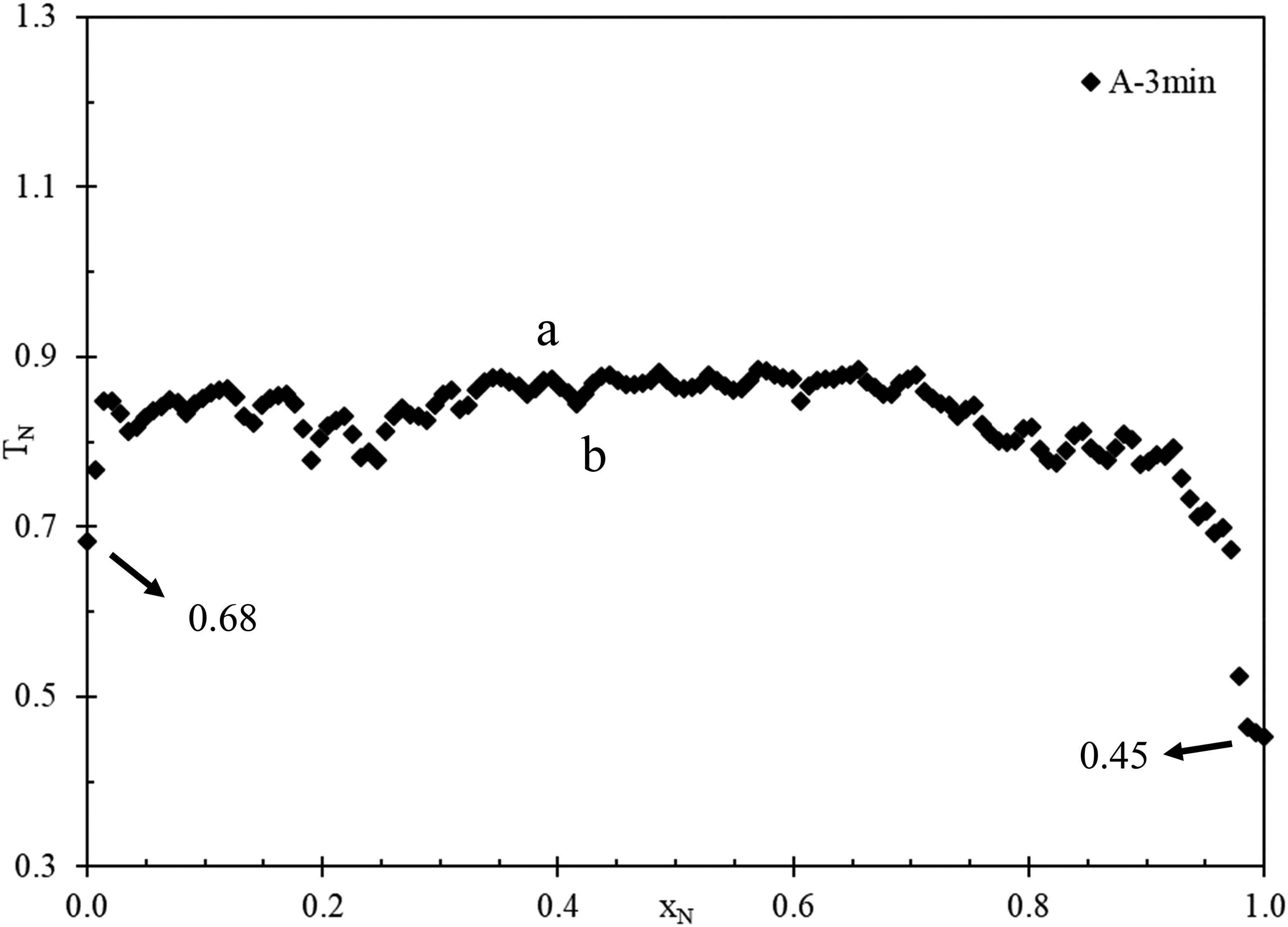
Measured IR temperature distribution across the flat surface for coil A-3 min.

Figure 7 shows the measured IR temperature distribution across the flat surface of coil A at ∼12 min from the start of coiling (denoted by A-12 min). The temperature at all coil positions is relatively uniform (compared with A-3 min) due to the homogenisation of the overall coil temperature. In addition, the temperature at the inner surface of the coil increases from 0.68 T_N (A-3 min) to 0.86 T_N (A-12 min). This change is primarily attributed to the removal of the mandrel from the coil at ∼6 min from the start of coiling. Similarly, the temperature at the outer surface of the coil increases from 0.45 T_N (A-3 min) to 0.83 T_N (A-12 min) as heat from the bulk of the coil is conducted to the outer surface.

Figure 7.

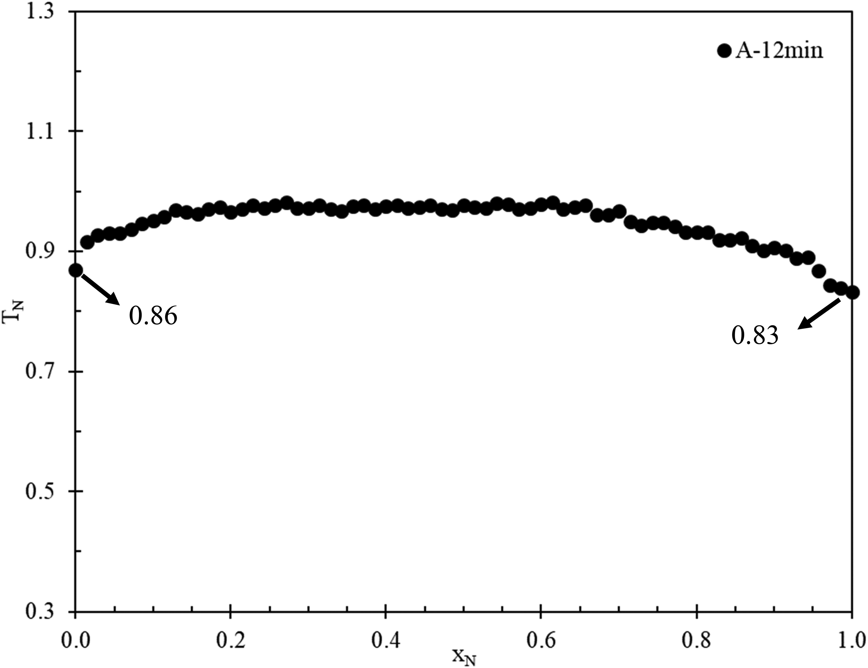
Measured IR temperature distribution across the flat surface for coil A-12 min.

Figure 8 shows the measured IR temperature distribution across the flat surface of all three coils at the start of coiling (denoted by 0 min) and ∼3 min from the start of coiling (denoted by 3 min). The temperature at the start of coiling is highest for coil A followed by coil B and coil C. There is a relatively large difference in temperature (shown by ΔT_BC in Figure 8) between coil B and coil C even though the target CIT for both coils was the same. After ∼3 min, the temperature across the flat surface for all three coils decreases (e.g., for coil A the average temperature decreases from 1.04 T_N to 0.79 T_N). The temperature for coil B remains higher than that for coil C between x_N= 0 and x_N= 0.8, which correlates well with the initial temperature distributions of coils B and C.

Figure 8.

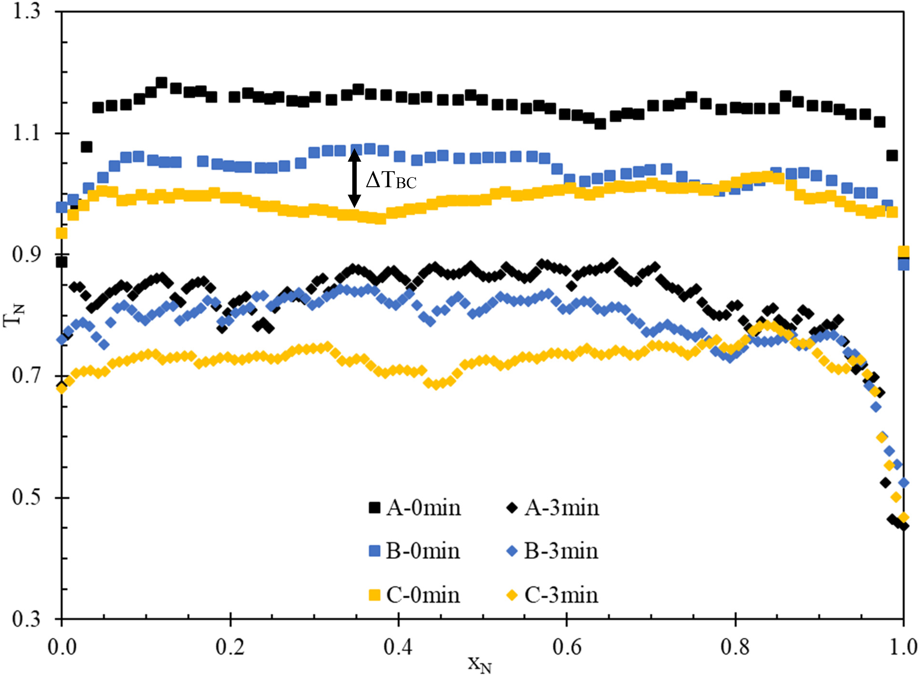
Measured IR temperature across the flat surface of all three coils at the start of coiling (0 min) and ∼3 min from the start of coiling (3 min).

Figure 9 shows the measured IR temperature distribution across the flat surface of all three coils at ∼12 min from the start of coiling (denoted by 12 min). The overall temperature is highest for coil A followed by coil B and then coil C. The temperature difference between coils B and C, from x_N= 0 to x_N= 0.8, becomes lower than that at the beginning of coiling. This is due to temperature homogenisation across the individual coils over time. The relative temperature differences across the flat surface of the three coils correspond well with the initial temperature distribution of the three coils.

Figure 9.

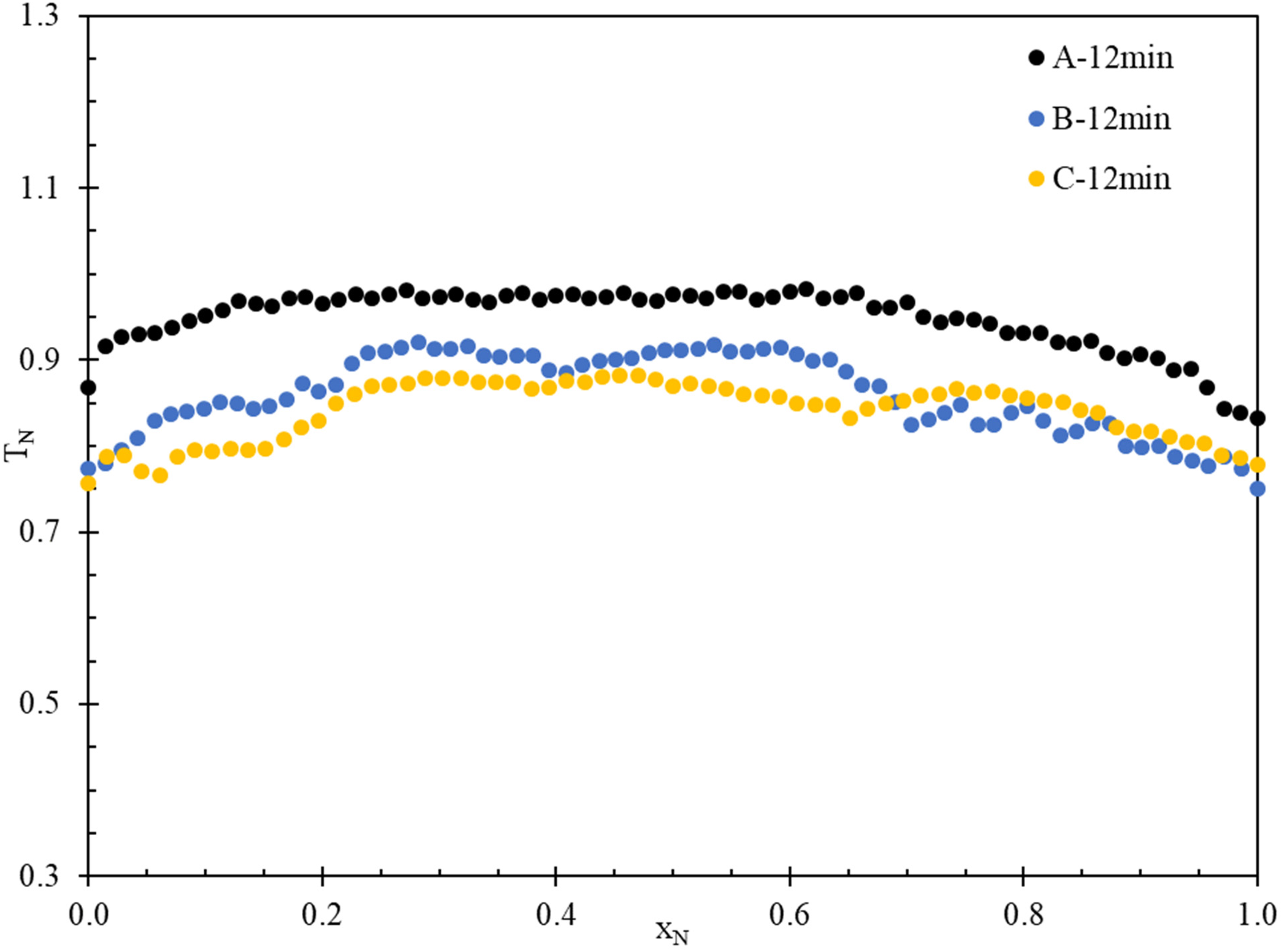
Measured IR temperature distributions across the flat surface for coils A-12 min, B-12 min and C-12 min.

Thermal model validation

Figure 10 compares the measured IR temperature distributions across the flat surface with the predicted values (FE model) for the three coils at 3 min and 12 min from the start of coiling. The local temperature fluctuations (Figure 6) in the experimental profiles are not present in the model as the model does not account for the interface between each coil layer. Overall, the predicted temperatures compare well with the measured temperatures.

Figure 10.

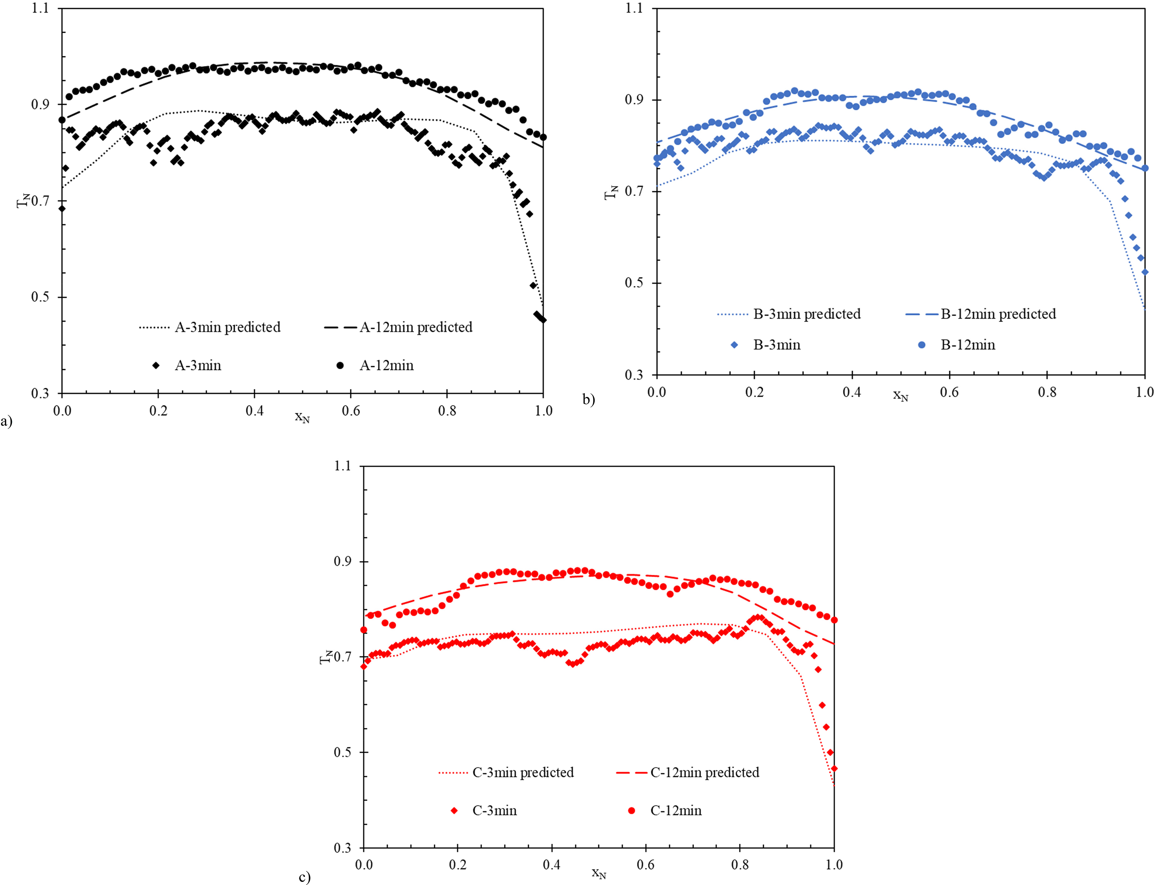
Comparison of the temperature distribution predicted from the FE thermal model and the measured temperature distributions from the IR measurements coil (a) A, (b) B and (c) C at 3 min and 12 min from the start of coiling.

Thermal model predictions of temperature–time profile in the coils

The temperature–time profile was predicted at three (3) selected coil/skelp locations (labelled 1, 2 and 3) and is shown schematically in Figure 11. Location 1 is near the inner surface of the coil which was close to the mandrel, location 2 is at the central radius location of the coil and location 3 is near the outer surface of the coil. All three locations are a quarter length away from the flat surface of the coil, which corresponds to the points being a quarter width away from the edge of the skelp. In addition, locations 1, 2 and 3 are at x_N= 0.05, 0.5 and 0.95, respectively. The corresponding locations on the coil are also shown in Figure 11.

Figure 11.

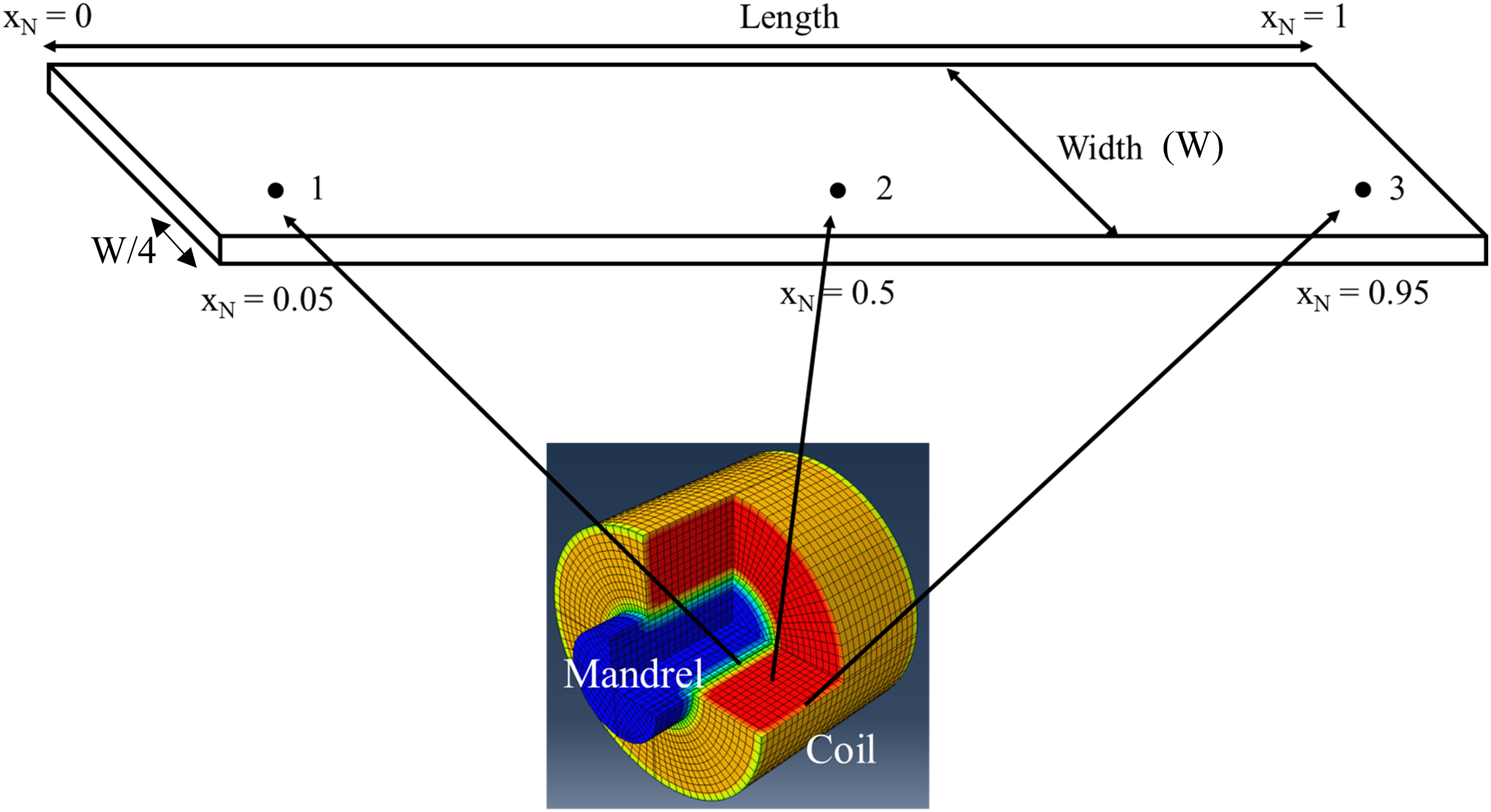
Selected locations for predicted temperature–time profile comparison.

Effect of non-uniform skelp temperature before coiling

The predicted temperatures for locations 1, 2 and 3 for coil A from the start of coiling to 30 min after the start of coiling are shown in Figure 12. Location A-1 (location 1 for coil A) exhibits faster cooling compared with both locations A-2 and A-3 during the initial coiling stage (t < ∼2 min) due to conduction cooling by the mandrel. Following mandrel removal (∼6 min), the temperature at location 1 starts to increase as heat from the bulk of the coil is conducted outwards. Location A-3 shows faster cooling compared with locations A-1 and A-2 for ∼2 to ∼5 min and this is attributed to enhanced applied cooling. After the end of enhanced cooling (∼5 min), the temperature at location 3 begins to increase as heat from the bulk of the coil is conducted outwards. Location A-2 shows a decrease in temperature with the slowest cooling rate. There is a small increase in the temperature at location A-2 during the first 10 min. This is due to local regions of the skelp (corresponding to x_N= 0.4) with higher initial temperature (1.17 T_N at x_N= 0.4 compared with 1.14 T_N at x_N= 0.5). This shows that the initial skelp temperature profile is essential in estimating the temperature–time profiles at different locations within a steel coil.

Figure 12.

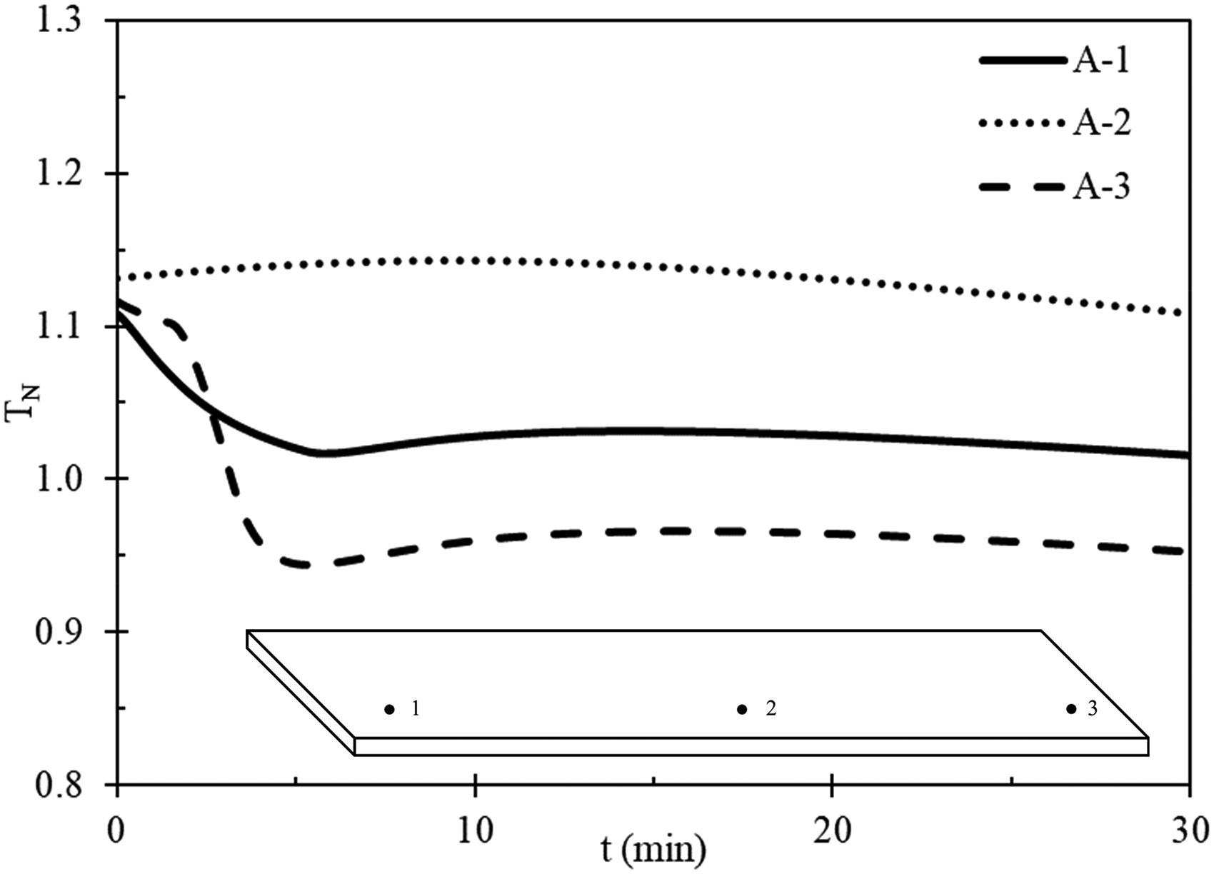
Predicted temperatures at locations 1, 2 and 3 for coil A from coiling start (t = 0) to t = 30 min.

The predicted temperatures for locations 1, 2 and 3 for coil A up to 1200 min are shown in Figure 13. The temperatures at locations 1 and 3 also start to decrease after 30 min. This is because the rate of heat loss from the coil surfaces due to radiation and convection is greater than the rate of heat transfer from the bulk of the coil towards the surface due to conduction. As the coil surface temperature decreases, the rate of heat loss from the coil surfaces due to radiation and convection decreases. At the same time, as the temperature within the coil homogenises, the rate of heat transfer from the bulk of the coil towards the surface also decreases. This results in a decreased cooling rate across the coil over time. After ∼10 h, the rate of heat transfer from the coil surfaces becomes equal to the rate of heat transfer from the bulk of the coil towards the surface. This results in homogenisation of the temperature across the coil (temperature differences at all three locations become less than 10 °C) and in a constant cooling rate for the overall coil.

Figure 13.

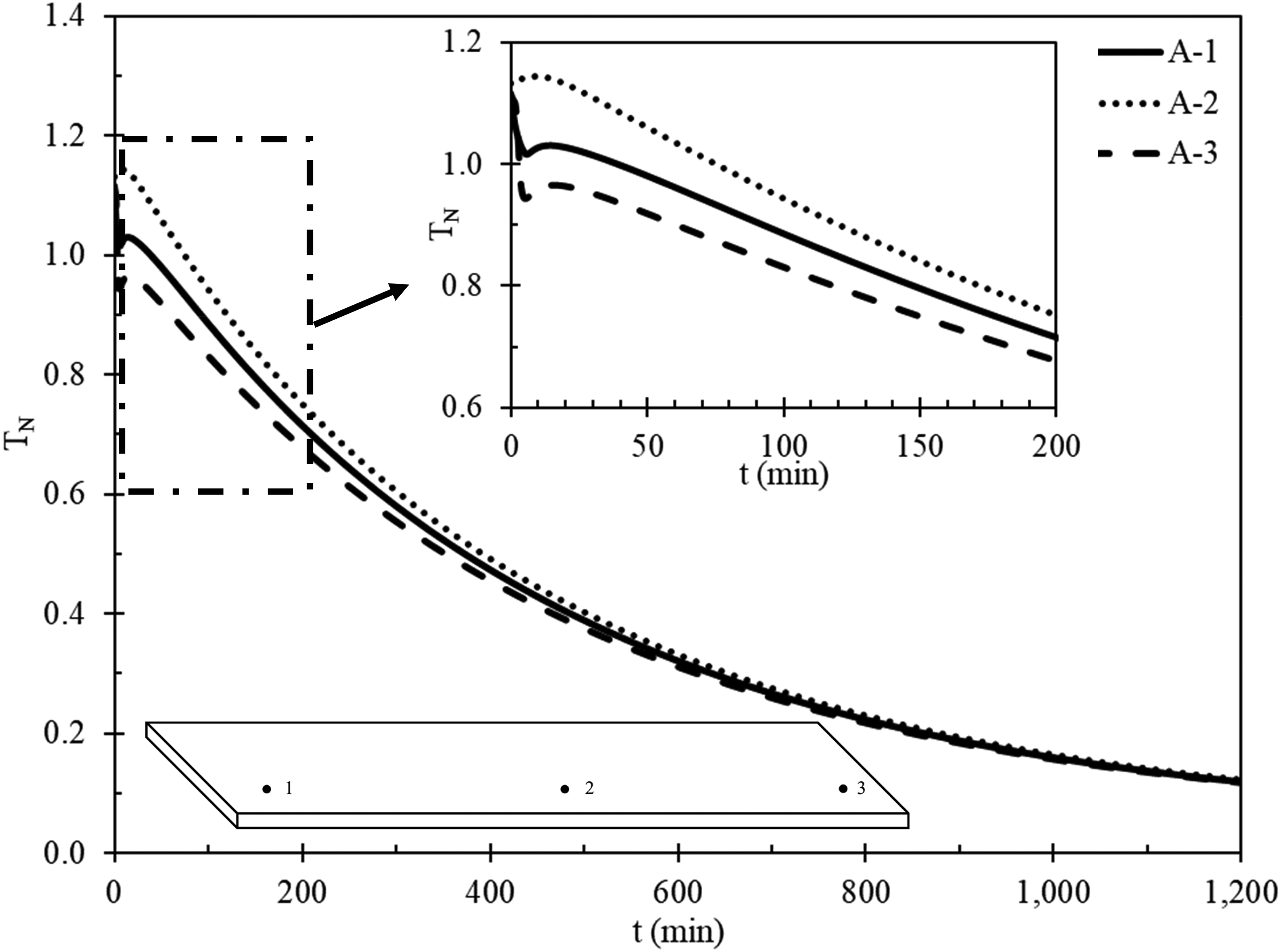
Predicted temperatures at locations 1, 2 and 3 for coil A from coiling start (t = 0) to t = 1200 min.

Effect of initial skelp temperature on coil cooling

The predicted temperatures at location 3 for coils A, B and C up to 30 min from the start of coiling are shown in Figure 14. The predicted temperature at location 3 for coil A is the highest followed by coils B and C. This correlates well with the initial temperature of the coils. Location 3 shows a similar trend in temperature for all coils (faster cooling for ∼2 to ∼5 min due to enhanced applied cooling and an increase in temperature after the end (∼5 min) of enhanced cooling).

Figure 14.

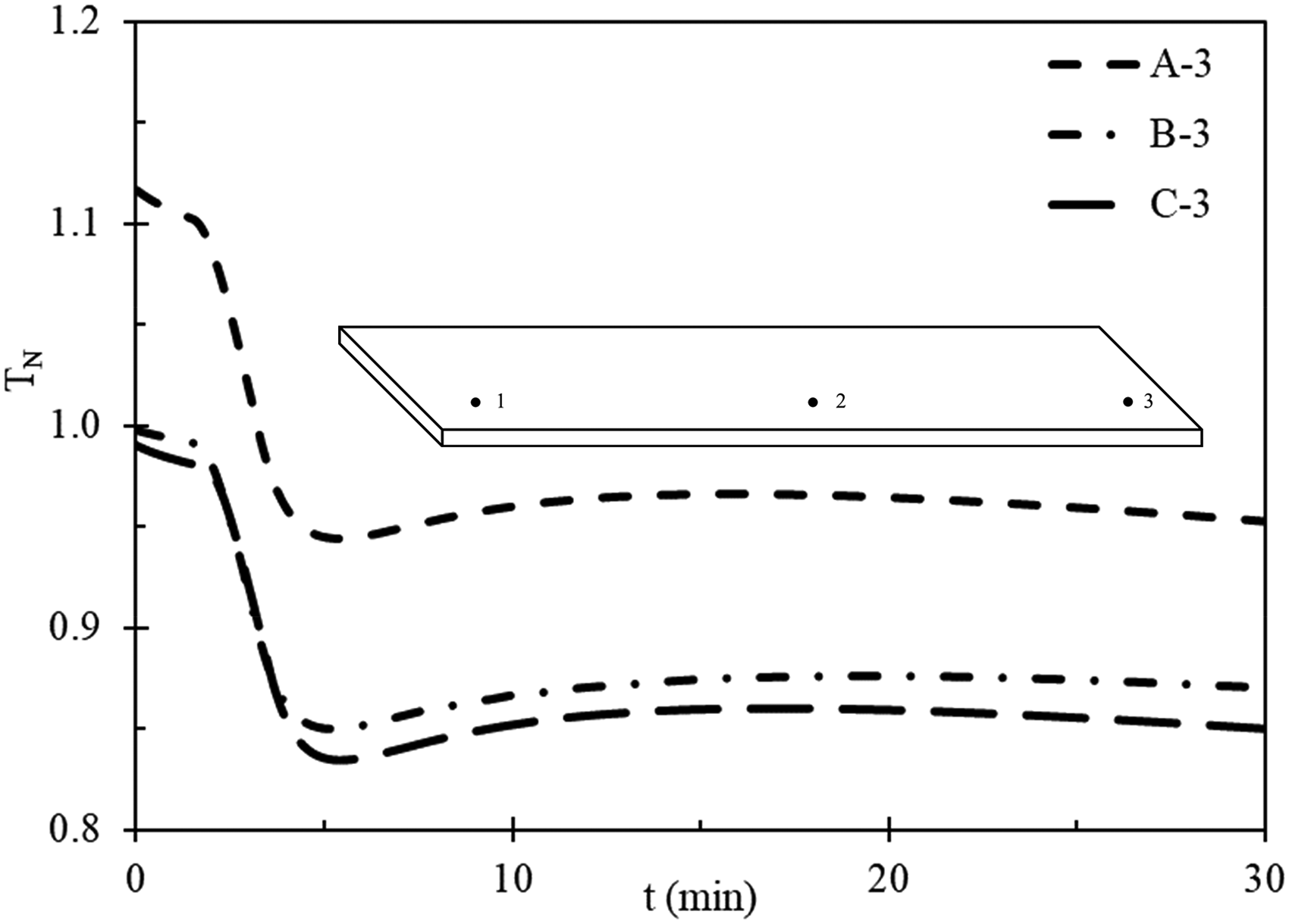
Predicted temperatures at location 3 for coils A, B and C from the start of coiling.

The predicted temperatures at location 3 for coils A, B and C up to 1200 min from the start of coiling are shown in Figure 15. The predicted temperature for all three coils converges (temperature difference for all three coils becomes less than 10 °C) in about 10 h (∼600 min) from the start of coiling. The decrease in temperature is higher for coil A compared with coils B and C. This is attributed to a higher cooling driving force for coil A since coil A had a higher initial temperature. Therefore the effect of initial coiling temperature remains only up to ∼10 h from the start of coiling (Figure 15).

Figure 15.

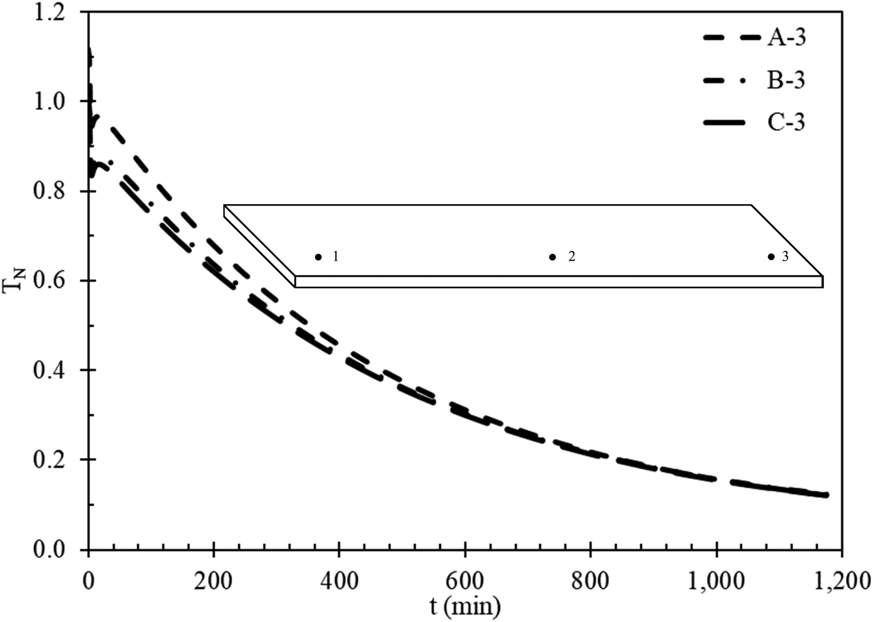
Predicted temperatures at location 3 for coils A, B and C from the start of coiling.

Thermal model application

The thermal model was used to quantify the effect of initial skelp temperature distribution on coil cooling at coil locations 1, 2 and 3 in Figure 11. Figure 16 shows the measured skelp temperature as a function of x_N and the skelp temperature for a hypothetical temperature profile A-II-0 min in which the temperature of both the head and tail ends of the skelp are higher than the average temperature, instead of lower which was the case for the as-measured conditions. The thermal simulations for both A and A-II were run using identical boundary conditions.

Figure 16.

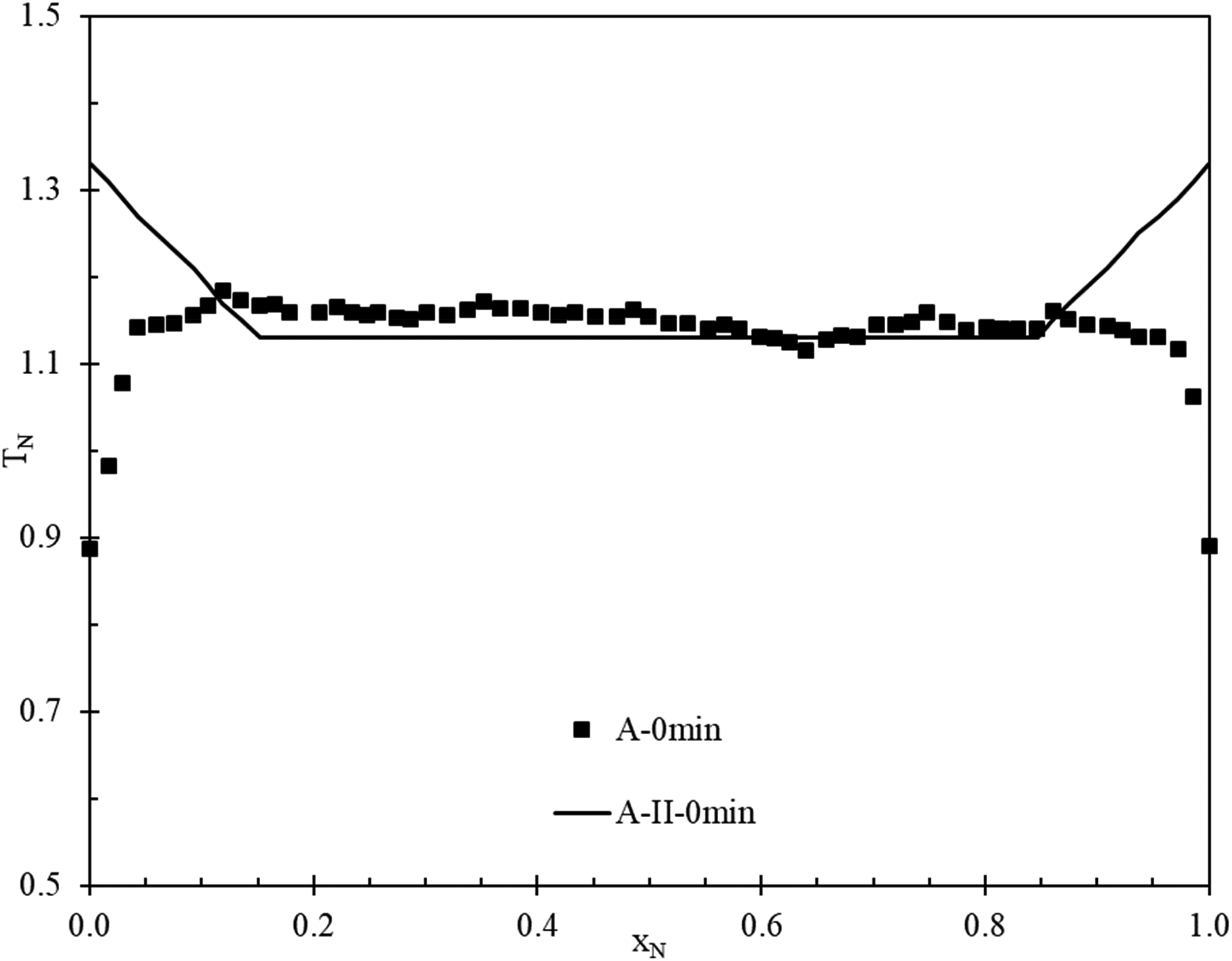
Initial temperature variations for skelp A.

Figure 17 shows the predicted temperature–time profile at skelp locations 1 and 3 for both A and A-II. Due to the higher initial temperature, A-II-1 and A-II-3 show a significantly higher temperature in the coil than A-1 and A-3. This difference becomes less than 10 °C after 60 min from the start of coiling. This simulation scenario shows that the temperature distribution along the length of the skelp can influence the temperature in the early stages of coiling and, potentially, the kinetics of carbide precipitation.

Figure 17.

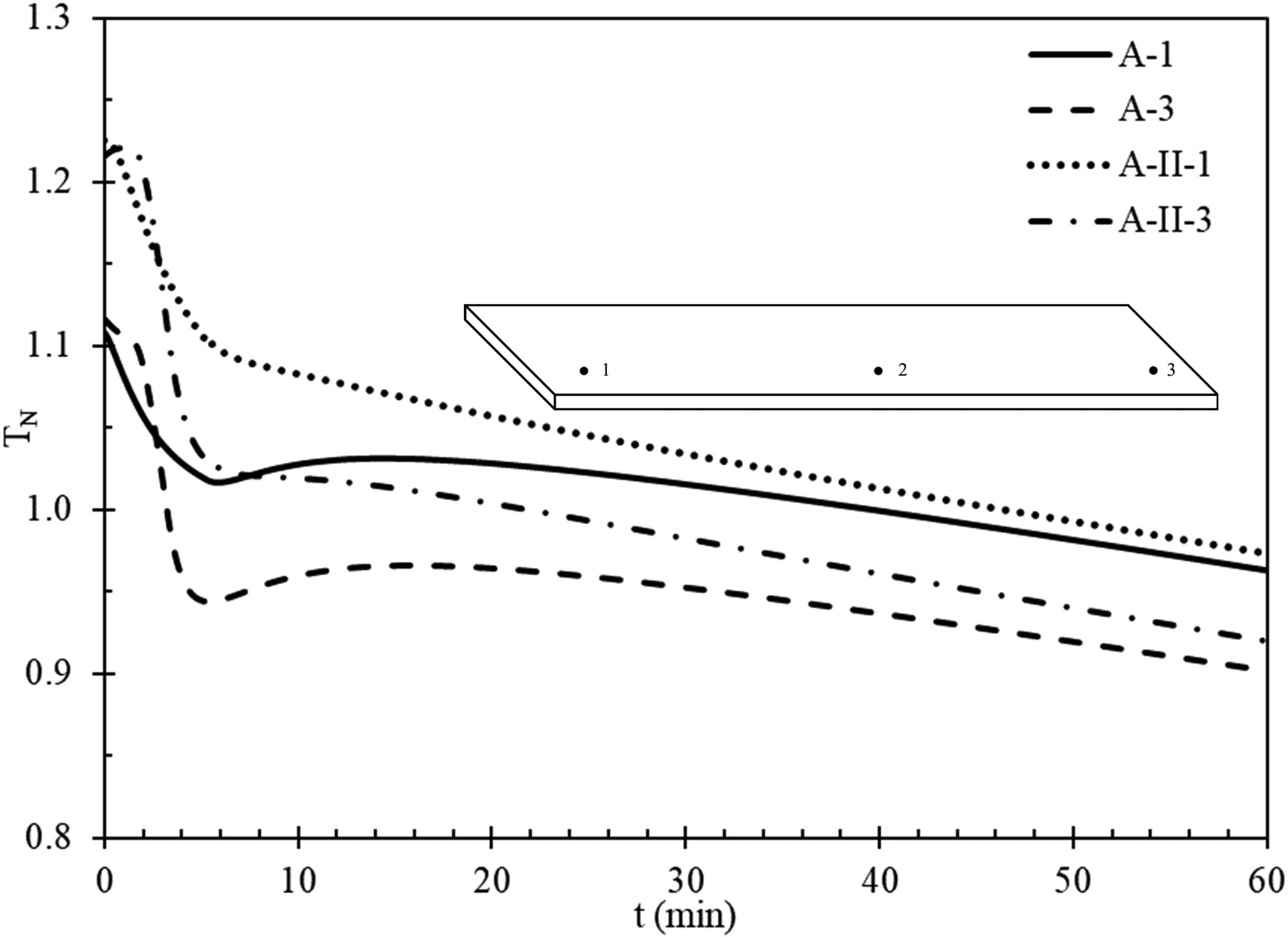
Predicted temperatures at locations 1 and 3 for A and A-II.

Conclusions

In this work, the effect of skelp temperature on coil cooling was studied. Coil cooling was modelled by including the effect of non-uniform skelp temperature prior to coiling. The main conclusions are as follows:

A difference in skelp thickness (19 mm vs. 25 mm) does not affect the cooling of steel coils; however, the skelp temperature distribution (along the length of the skelp) prior to coiling has a significant impact.

The thermal model shows that the near-surface regions of the coils experience faster cooling, with a temperature difference of up to 60 °C compared with the central regions of the coils. This difference can affect the local microstructure and ultimately result in inhomogeneous mechanical properties. The difference in coil temperature (at all points) due to a difference in skelp temperature becomes small (<10 °C) in the coil after ∼10 h.

The difference in cooling experienced by the different regions in a coil can be minimised by controlling the skelp temperature prior to coiling. A higher temperature (∼50 °C) near the head and tail regions of the skelp results in a lower difference (a difference of ∼10 °C instead of ∼50 °C) in cooling experienced by the near-surface regions.

Footnotes

Acknowledgements

The authors would like to acknowledge the Natural Sciences and Engineering Research Council (NSERC) of Canada and Evraz Inc. NA for providing financial support and opportunity for conducting the temperature measurements. Also, we are grateful for Riley Dobrohoczki who aided with the mill measurements.

Declaration of conflicting interests

The authors declared no potential conflicts of interest with respect to the research, authorship and/or publication of this article.

Funding

The authors received no financial support for the research, authorship and/or publication of this article.

ORCID iDs

Rishav Raj

Michael J. Gaudet

Appendix

Figure 18 shows the mesh size convergence test for the thermal model. Global mesh size of 0.04 m was used for the current work.

Sensitivity analysis:

The effect of variation in thermal conductivity and heat capacity values on the predicted temperature profile at location A-1 is shown in Fig. 19. The effect of interfacial layers in the coils is modelled using an equivalent thermal conductivity approach,^8,9,14 which includes the thermal resistance due to gap present in between consecutive coil layers. Karlberg et al.⁹ showed that the interfacial coil layers can reduce the overall steel conductivity by up to 8 W/mK. The sensitivity analysis included here (case k-10) also captures the effect of interfacial layers. A starting time step of 0.01 s was used with a minimum time step value of 0.001 s. The default automatic time step incrementation option available in ABAQUS was employed. A maximum temperature difference limit of 1 °C between two consecutive time steps was used.

References

Sajadi

Ahmadi Brooghani

. Experimental and Numerical Investigation of Through-Thickness Mechanical Properties in Api X65 Line Pipe Steel. Available at SSRN 4158157.

Baker

. Microalloyed steels. Ironmaking Steelmaking 2016; 43: 264–307.

Gao

Leng

, et al. Effects of niobium and heat treatment on microstructure and mechanical properties of low carbon cast steels. Mater. Des. 2016; 105: 114–123.

Challa

VSA

Zhou

Misra

RDK

, et al. The effect of coiling temperature on the microstructure and mechanical properties of a niobium–titanium microalloyed steel processed via thin slab casting. Mater. Sci. Eng. A 2014; 595: 143–153.

Wang

Deng

, et al. The determining role of finish cooling temperature on the microstructural evolution and precipitation behavior in an Nb-V-Ti microalloyed steel in the context of newly developed ultrafast cooling. Metall. Mater. Trans. A 2016; 47: 1929–1938.

Park

Hong

Baik

, et al. Finite element analysis of hot rolled coil cooling. ISIJ Int. 1998; 38: 1262–1269.

Saboonchi

Hassanpour

. Heat transfer analysis of hot-rolled coils in multi-stack storing. J. Mater. Process. Technol. 2007; 182: 101–106.

Karlberg

. Thermo-mechanically coupled isotropic analysis of temperatures and stresses in cooling of coils. ISIJ Int. 2016; 56: 1808–1814.

Karlberg

. Modelling of the temperature distribution of coiled hot strip products. ISIJ Int. 2011; 51: 416–422. Lewis, R. W., Morgan, K., Thomas, H. R., & Seetharamu, K. N. (1996). The finite element method in heat transfer analysis. John Wiley & Sons.

10.

Weisz-Patrault

Legrand

Deka

., et al. (2022, October) Thermo-mechanical Coil Cooling Model to Tackle Shape and Mechanical Properties Issues after Hot Rolling of Steel Sheets. In: 12th international rolling conference.

11.

Ilmola

Pohjonen

Koskenniska

, et al. Coupled heat transfer and phase transformations of dual-phase steel in coil cooling. Mater. Today Commun. 2021; 26: 101973.

12.

Liu

Shi

, et al. Experimental investigation of emissivity of steel. Int. J. Thermophys. 2013; 34: 496–506.

13.

Wen

. Investigation of steel emissivity behaviors: examination of multispectral radiation thermometry (MRT) emissivity models. Int. J. Heat Mass Transfer 2010; 53: 2035–2043.

14.

Saboonchi

Hassanpour

Hajiannezhad

. Estimation of thermal stresses in hot-rolled steel coils during natural air cooling. J. Therm. Stresses 2010; 33: 521–532.

15.

Tian

Zhang

, et al. The effect of laminar cooling heat transfer coefficient on the temperature field of steel plate (Retraction of Vol 48, Pg 1076, 2021). 2024.

16.

Karl

. Integrated Computational Modeling of Run-Out Table Phase Transformations. 2023.

17.

Pelzmann

Dupont

Sauté

, et al. Two-color pyrometry for backface temperature and emissivity measurement of burning materials. Int. J. Therm. Sci. 2023; 184: 107894.

18.

Sadiq

Wong

Tashan

, et al. Determination of steel emissivity for the temperature prediction of structural steel members in fire. J. Mater. Civ. Eng. 2013; 25: 167–173.