
Abstract
The assessment of prognostic markers is key to the improvement of therapeutic strategies for cancer patients. Some promising markers may fail to be applied in clinical practice, or some useless markers may be applied, because of misleading results ensuing from inadequate planning of the study and/or from an oversimplified statistical analysis. This commentary illustrates and discusses the main issues involved in planning an effective clinical study and the subsequent statistical analysis for the prognostic evaluation of a cancer marker. Another aim is to extend the most applied statistical models (ie, those using Kaplan-Meier and Cox) to enable the choice of the best-suited methods for study endpoints. Specifically, for tumor-centered endpoints like tumor recurrence, the issue of competing risks is highlighted. For markers measured on a continuous numerical scale, a loss of relevant prognostic information may occur by setting arbitrary cutoffs; thus, the methods to analyze the original scale are explained. Furthermore, because the P-value is not a sufficient criterion to assess the usefulness of a marker in clinical practice, measures for evaluating the ability of the marker to discriminate between “good” and “bad” prognoses are illustrated. Several tumor markers are considered both in human and veterinary medicine. Given the similarity between markers for human breast cancer and canine mammary cancer, an application of the statistical methods discussed within the article to a public dataset from human breast cancer patients is shown.
Keywords
Research on the clinical characteristics and pathological tumor features of oncology patients is aimed at a better understanding of tumor biology, to advance diagnosis and open new treatment protocols with the final aim to improve prognosis. Although results of current research may seem promising, patient responses to anticancer therapies as well as their life expectancy are still heterogeneous for the same tumor types. Inconsistencies between histopathological features and prognosis have been documented in several canine tumors. This suggested that the classical clinicopathological factors and histopathological criteria are not enough to accurately predict the prognosis and response to therapy of the tumor. 31 Clinical and pathological characteristics are combined to identify patient groups with different disease progression or treatment response or to propose amendments of the World Health Organization (WHO) staging system (see, eg, Liu et al, 29 Bell et al, 5 Winick et al, 49 Horta et al, 23 Im et al 24 ). This is not surprising, as risk groups could be useful to plan first-line treatments (eg, to avoid the potential overtreatment of low-risk patients and/or undertreatment of high-risk patients) or to select patients for clinical trials including novel therapeutic principles and protocols according to their health status and probability of treatment response.
The more information available on each specific tumor entity, the greater the possibility of building more effective patient stratification. The addition of novel histopathologic tumor characteristics to other clinical and pathologic variables has become a frequent approach because it improves the identification and stratification of cancer patients in different risk groups. To show the methodology for assessing novel tumor characteristics, we refer to a broad definition of tumor markers as heterogeneous variables measured either in categorical or continuous scales, which are frequently evaluated for prognostic aims. According to the definition given by the National Cancer Institute, a tumor marker should be anything present in or produced by neoplastic cells or other cells of the body in response to cancer or certain benign (noncancerous) conditions that provide information about cancer, such as how aggressive it is, whether it can be treated with targeted therapy or whether it is responding to treatment. Tumor markers have traditionally been proteins or other substances that are made by both normal and cancer cells but at higher amounts by cancer cells. These can be found in the blood, urine, stool, tumors, or other tissues or bodily fluids of some patients with cancer.
32
Several tumor markers are considered both in human and veterinary medicine. For example, biomarkers in human breast cancer are also detectable in canine mammary tumors. As a consequence, it is recognized that the most studied and reliable biomarkers of canine mammary tumors are the same as human breast cancer 27 ; for example, Ki-67, endothelial growth factor receptor, epidermal growth factor receptor 2 (HER-2), estrogen receptor, progesterone receptor, and cyclooxygenase 2 (COX-2). For these reasons, methodological approaches for evaluating the prognostic and predictive role of human biomarkers are useful also to study animal tumor markers.
Human and veterinary oncological research are ongoing, and the contribution of tumor markers in body fluids and tumor tissues is investigated either to explain a patient’s overall survival regardless of their correlation to therapy (prognostic) or to give information on a therapeutic intervention (predictive). 34 To such ends, longitudinal studies must be conducted. In these studies, the time to occurrence of tumor-related events (eg, local recurrence and distant metastases) and death (together with the cause of death) are recorded for each patient. The prognostic or predictive role of tumor markers is investigated by statistical methods specific for time-dependent events (survival analysis).
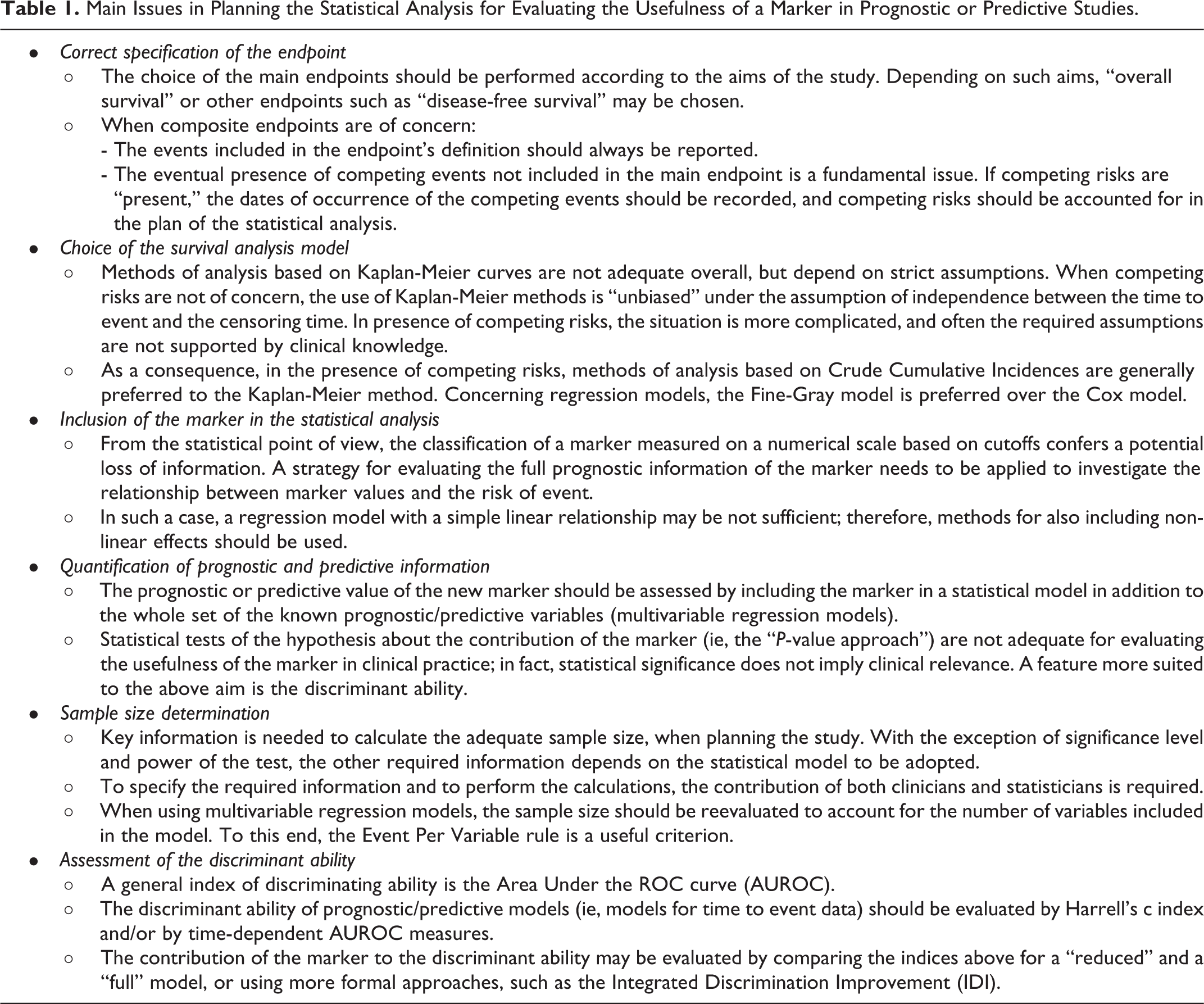
Due to the high number of papers available in the literature about prognostic tumor markers, we can argue that many clinicians and pathologists are currently involved in longitudinal studies aimed at evaluating a marker’s prognostic value. Most study investigators are aware of the importance of the application of adequate statistical approaches to obtain reliable results, but this requires specific statistical know-how, which is not widespread among researchers with clinical and/or biological training. The main aims of this work are to provide a commentary tailored for clinical and biological researchers of the major issues pertinent to the planning of statistical analysis, and to present some adequate statistical methods for the assessment of prognostic and predictive value of markers. A sketch of the topics discussed throughout the article is reported in Table 1. In the presentation of the topics, we avoid the use of mathematical formulas, which could hamper the understanding without adding information directly useful to the readers.
Main Issues in Planning the Statistical Analysis for Evaluating the Usefulness of a Marker in Prognostic or Predictive Studies.
Two features are fundamental to the application of all the statistical methods considered in this work: namely, large sample size and the availability of a marker measured on a continuous scale. As far as we know, a dataset from veterinary studies with these characteristics is not currently available in public repositories. Given the similarity between markers for cancer of the mammary gland in humans and dogs, we used a real-data example in which the statistical methods are applied to a public dataset from women with breast cancer on a large case series. The example shows statistical topics, methodologies, and problems that may be faced also in veterinary longitudinal studies. We are aware that often the sample size reached in veterinary tumor studies is smaller than that provided here. Nonetheless, adequate sample size is required for obtaining reliable results from a comprehensive statistical evaluation of potential prognostic/predictive markers. To this aim, multicenter clinical studies could be considered for obtaining robust and reliable evaluation.
Correct Specification of the Endpoint
In longitudinal studies, the endpoint is the time elapsed from the patient’s entry into the study (eg, the date of starting treatment) to the time of occurrence of the events of interest. Overall survival is considered the most relevant endpoint for the evaluation of “patient-centered” treatment efficacy. 11,48 Its definition is simple and unambiguous, because all causes of death are included in the endpoint. In veterinary studies, death for euthanasia is included together with the other causes of death. It is worth noting that the choice of euthanasia is often related to the worsening of life quality caused by the disease, which leads to the decision of euthanasia. In human studies, euthanasia does not occur and the causes of death are considered together, regardless of whether they are directly or indirectly related to the tumor, or other diseases related to aging.
Alternatively, “tumor-centered” endpoints are frequently chosen as the main endpoint. These endpoints usually include disease-free survival, progression-free survival, and relapse-free survival. They combine groups of events selected among tumor progression, local and distant tumor recurrence, metachronous cancer, severe toxicity, and death, and thus, they are called “composite” endpoints. The respective time of occurrence is the time elapsed from the beginning of follow-up to the occurrence of the first of the events of interest. It is worth noting the lack of general agreement about the definition of composite endpoints reported in the literature. This may impede the cross-comparison of results of different studies; thus, endpoints should be always accurately defined.
It is unlikely that the endpoint of interest may be observed in every patient included in the study. In particular, for patients who are alive without any event recorded before the end of the study or who are lost to follow-up without events, the time of occurrence is considered as “censored” at the date of last clinical information (censoring date). In such cases, the endpoint may occur after the censoring date, but the date of occurrence is unknown (right censoring). A different situation arises when the endpoint includes only a subset of the possible events. For example, death for all causes can be subdivided into distinct endpoints, usually “death related to the disease” and “not related to the disease,” and a single cause may be classified as “related” or “unrelated” depending on the clinicians’ judgment. For study aims, oncologists are mainly interested in death related to disease, but this cannot be observed in every subject: in particular, it cannot be observed if subjects die for causes not related to the disease. This provides an example of “competing risks”: death for other causes “compete” with death related to the tumor. In general, competing risks are said to be present when a patient is at risk of 2 or more events, and the occurrence of one of these events prevents the occurrence of the others. 12 For some tumor-centered endpoints, some events not included in the main endpoint could be competing events. Consider, for example, a main endpoint including only tumor relapse. In this case, the occurrence of death without tumor relapse prevents the observation of the main endpoint; this is another example of competing risks.
It should be stressed that the occurrence of a competing event can be viewed as a peculiar kind of censoring, but the two concepts are distinct. In fact, in the case of censoring, the subject is considered at risk for the event of interest (because it is not known if the event will occur in the following time and, if so, when it will occur), while in the competing risks setting, the event of interest is “prevented” when a competing event occurs.
Choice of the Survival Analysis Model
In longitudinal studies the initial statistical analysis is commonly based on the Kaplan-Meier method. This method provides estimates of the probability to be free of the endpoint of interest at any given follow-up time (survival curve). The comparison of survival curves among distinct groups is performed by the log-rank test. A representation alternative to survival curves is provided by the cumulative incidence, that is, the probability of event occurrence at a time less or equal to any given follow-up time. Estimates of cumulative incidence are easily obtained by calculating, for each time t, one minus the estimate of the survival probability at that time.
The Kaplan-Meier method is based on strict assumptions; thus, its use is not correct for every endpoint. As a consequence, biased results may derive from a wrong modeling strategy. For overall survival, and for relapse-free survival (when the composite endpoint includes all the possible tumor-related events and death), the Kaplan-Meier method is adequate only under the assumption that the time to censoring and the time-to-event are independent. As an example: for overall survival, the above assumption implies that patients alive who are lost to follow-up share the same “future” survival probability with those patients who are still in follow-up. This assumption can be “realistic” for patients who are lost to follow-up for reasons not depending on their health status; conversely, if the reasons are related to health status (a typical example: a patient has severe side effects make it impossible to continue the treatment), then it is unlikely that the survival probability of the censored patient is the same as the survival probability of patients that are still participating in the study.
When competing risks are present, a strategy of analysis sometimes adopted is to consider the time to occurrence of the competing events (eg, death without tumor recurrence) as a censored time, and to estimate the survival curves of the event of interest (eg, recurrence) by the Kaplan-Meier method. This is adequate only under the assumption that the probability of death is independent of the probability of recurrence, which may not always be tenable according to clinical experience. In general, some patients may be lost to follow-up by being free from any event. The assumption that these patients share the same probability of event occurrence with patients who are still in follow-up is still necessary, but the situation is more complex. As an example, suppose that we are interested in “tumor relapse-free survival” where only tumor-related events are of concern (death is not included in the endpoint). Some patients may die for unrelated tumor causes before a tumor relapse is observed. The independence between times to death and time to relapse is doubtful: if the patient was not deceased, could we suppose he/she will have the same “relapse-free probability” as patients with observed relapse?
It must be stressed that in the presence of competing risks, the interpretation of the survival curve is not straightforward. As an example, tumor relapse-free survival (ie, the probability of being free from tumor recurrence) corresponds to the sum of two probabilities: the probability of being alive without tumor recurrence, plus the probability of being deceased without recurrence. For this reason, it is preferable to avoid survival probabilities and instead estimate crude cumulative incidences (ie, the probability of occurrence of an event at any given follow-up time t, that accounts for the presence of competing risks). Comparisons between crude cumulative incidences among groups should be performed by the Gray test. 14
Concerning regression models, the Cox model is the most commonly used to evaluate joint covariate effects on overall survival and relapse-free survival where the composite endpoint includes all kinds of tumor relapses and death. In presence of competing risks, the Fine and Gray model 10 should be used instead of Cox (see, eg, Kim, 28 Satagopan et al, 39 Oyama et al 35 ). Competing risk analysis tools are available in statistical software such as R, STATA, and SAS.
Inclusion of the Marker in the Analysis
Several markers are measured on a qualitative (ordered) scale or a quantitative (numerical) scale. The measurement method and the scale of a marker are decided using criteria established by the lab responsible according to their scientific skill. From the point of view of statisticians, to exploit the maximum potential predictive/prognostic role of the marker, it is preferable to maintain its original scale of measurement. Usually, a first exploratory evaluation is performed by “univariate” analysis. This is simple when the marker is recorded on a qualitative scale with only a few levels: for example, HER2 immunohistochemical expression can be scored on a qualitative scale from 0 to 3+ based on an interpretation of staining intensity, levels 0 and 1+ can be eventually grouped and classified as negative, and 2+ and 3+ can be grouped as positive (see, eg, Campos et al 6 ). In fact in such cases survival or cumulative incidence curves can be traced for each marker level. By the examination of the curves, it is possible to evaluate if some marker levels that show similar prognostic/predictive behavior could be grouped together. However, this approach is not feasible when markers are measured on a quantitative scale with several levels.
A widely used approach is to subdivide the scale so that “high” and “low,” or “high,” “medium,” and “low” risk groups are identified. This can be performed according to criteria defined in previous studies on the same or similar diseases; in absence of any previously established criterion, a specific and precise definition provided by the authors before they can begin data analysis can be used. The advantages of grouping are the ease of interpretation of the results, and the possibility of making more straightforward recommendations on the use of the marker for prognostic/predictive aims. The major disadvantage is the potential lack of prognostic/predictive efficacy.
As an example, estrogen receptor (ER) can be measured in fmol/mg of cytosolic proteins. The complete prognostic information is the ER content in the original measurement scale. If a cutoff is used, for example, 10 fmol/mg, to define ER− and ER+ classes, this implicitly leads to the assumption that every ER value within each of the two classes has the same prognostic role. This impedes evaluating whether ER in the original measurement scale could provide more accurate information about the prognosis.
Moreover, when data-driven rules are used to determine the risk groups, an additional disadvantage is that this generates different choices (cutoffs) in different studies, which makes it difficult to compare the published studies.
To maintain the original measurement scale for a numeric variable with several levels, a regression model is needed. How does it work? Let us consider the most popular model: the Cox model is based on the relationship between the levels of the marker and log(h(t)), that is, the logarithm of the hazard of the event at time t (the hazard is the rate of the event per time unit). The simplest kind of relationship consistent with the model is the “linear” one. Under the linear relationship, log(h(t)) increases for any increase of marker level, and the increase of log(h(t)) corresponding to an increase of x units of the marker is the same for each marker level. For example, suppose a marker M can assume levels from 0 to 10: the linear relationship implies that the ratio between the hazards for levels 4 and 5 is the same as the ratio between the hazards of levels 8 and 9 (Fig. 1). To provide a more clinically meaningful interpretation of the model, it is preferred to express hazard ratios using one marker level as the reference. As an example, Figure 2 shows the relative hazards obtained by setting 0 as reference level. In the figure, the hazard between level 5 of the marker and the hazard of the level 0 of the marker is 2.0, and the hazard between level 10 and the hazard of the level 0 is 4.0.
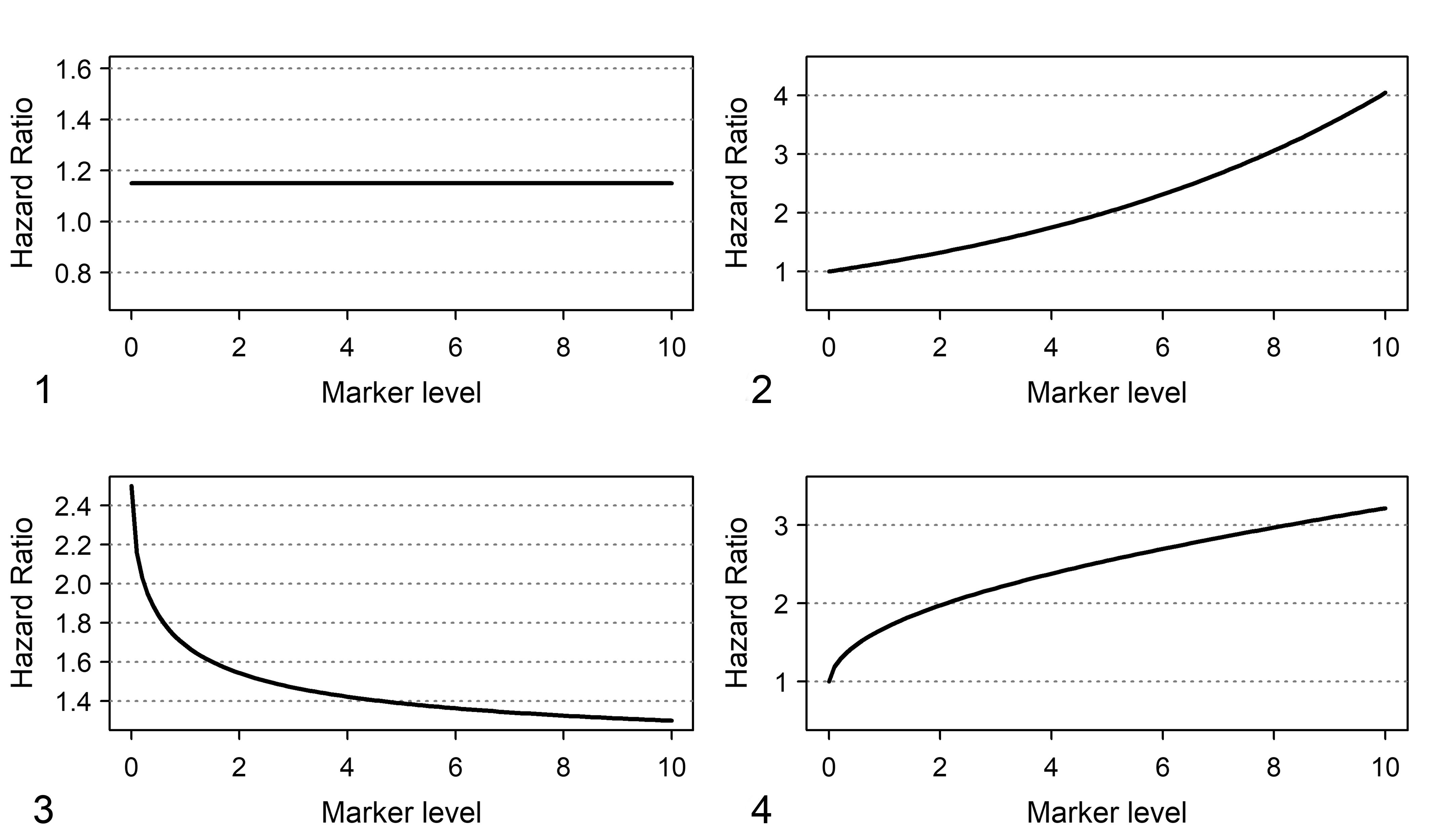
Shapes of hazard ratio functions for a linear and a nonlinear relationship between hazard and marker levels. Marker levels are placed on the X axis.
In this example, the linear relationship is simple and “user friendly”; however, it does not always fit the “real world.” For example, for some markers, a saturation effect is expected: it is expected that the increase of log(h(t)) corresponding to an increase of x units of the marker depends on the marker level, and the higher the marker level the smaller the increase of log(h(t)). An example is provided in Figure 3, where the ratio between the hazards for levels 2 and 1 is 1.7, and the ratio between hazard of levels 6 and 5 is 1.4. Figure 4 shows that a nonlinear relationship implies a distinct pattern of relative hazards that cannot be well fitted by a “linear” model. For example, the ratio between hazards of marker levels 2 and 0 is equal to 2.0, whereas the ratio between hazards of marker levels 6 and 0 is 2.7. Finally, effects more complex than those discussed in this example could occur and may be difficult to interpret.
Since the shape of the relationship between h(t) and marker levels provides insights about the role of the marker on disease progression dynamics, the convenience to categorize marker levels to create risk groups has to be evaluated with care. To provide an alternative to the use of empirical cutoff rules which are not based on the prognostic propensity of the marker (eg, median or other percentiles of the distribution), statistical procedures for “best” cutoff selection have been proposed (see, eg, Faraggi, and Simon, 9 Hilsenbach and Clark, 21 Mazumdar et al 30 ). Nevertheless, methodological papers in cancer journals advised against the “best cutoff” use mainly because of the risk of missing prognostic information or of obtaining unreliable results (see, eg, Altman et al, 2 Altman, 1 Holländer and Schumacher 22 ). In addition, the adoption of user-defined cutoff values was criticized also for methodological statistical papers. 38
Quantification of the Prognostic/Predictive Information Provided by the Marker
The assessment and quantification of the value of the new marker should be performed by adding the marker in a statistical model in which all the variables having a well-known prognostic/predictive role are included. To such an aim, the “P-value” corresponding to the marker is not sufficient. A statistically significant result does not imply a clinically relevant result and vice versa. In fact, it is easy to obtain a statistically significant result for an irrelevant prognostic impact of the marker if a large dataset is analyzed. Conversely, it is not easy to obtain statistically significant results for a clinically relevant prognostic impact of a marker if the sample has a small size. A statistically significant result depends on the power of the statistical test which, in turn, depends not only on the prognostic impact of the marker but also on sample size.
As an example, in the case of marker with a single cutoff, if the Kaplan-Meier survival curves for the two groups are significantly different, it can be interpreted that for each follow-up time, the proportion of surviving patients in one group is different from that of the other group. But this does not imply that each subject of one group has a different survival probability compared with each subject of the other group. For routine clinical practice, it is relevant to evaluate if the marker can discriminate subjects with different outcomes. This approach is applied to individual subjects rather than groups of subjects, and therefore is not assessed by the P-value, but by specific measures of “discriminant ability.” A P-value lower than 0.05 from the statistical test does not imply a satisfactory discriminant ability of the marker.
Sample Size Considerations for Statistical Tests
If statistical significance is considered a relevant criterion for the initial evaluation of the contribution of a marker, the sample size needs to be considered with care. The estimated sample size depends on the level of significance (usually 5%) but also on the power of the test (ie, the probability of obtaining a statistically significant result when the marker is effectively prognostic in the study’s target population). Usually, the power of the test is set to 80% or above.
A key issue is the choice of the minimal amount of prognostic impact considered clinically relevant to be detected by the test. For the sake of simplicity, let us consider the case of a marker classified into two classes (low and high) and prognostic impact evaluated by a univariate Cox model. The hazard ratio is the hazard of the event of interest in patients with high marker levels divided by that in patients with low marker levels. Once the level of significance and the power are defined, the magnitude of the hazard ratio must be set, by choosing the lowest hazard ratio that the study must be able to detect. Different methods are available to compute sample size for the Cox model. Each one requires different information on the incidence of the event at a given follow-up time (ie, the minimum follow-up time to be considered for the evaluation of marker effects, in which the majority of events are expected to be observed), the proportion of subjects within each group, the minimum hazard ratio to be detected, and, eventually, the expected percentage of censoring. According to one of the most cited papers, 41 the requested information is: the proportion of subjects in groups with low and high marker levels, the hazard ratio of the event, the hazard of the event in the group with low marker levels, the censoring rate, and the follow-up time.
For example, the investigator sets the study parameters as follows: a hazard ratio of 2 is chosen, the two groups are balanced (ie, 50% with low marker levels and 50% with high marker levels), the “baseline” hazard in the group with low marker levels is 0.071 (corresponding to a cumulative incidence of event of 1 − exp(−0.071*5) = 0.30 at 5 years of follow-up), the minimum follow-up is 5 years, and for sake of simplicity we assume no censoring. Using the above inputs, the calculation estimates that the total number of expected events at 5 years is 65 (41 and 24 in high and low marker level groups, respectively) and the estimated total sample size is 161 (81 and 80, respectively, for the 2 groups). Under the same scenario, if we set the percentage of censoring at 5 years at 5% (0.05), then the estimated sample size becomes 165. The calculations are shown in detail in Supplemental File S1 and can be reproduced using a freely available calculator (https://sample-size.net/).
It is the responsibility of clinicians to provide a relevant value for the hazard ratio to be detected, the expected proportion of events in the reference group (the group with low marker levels, in our example), and the censoring percentage. It is the responsibility of statisticians to apply correct methods and formulas for sample size calculation. However, when the marker is novel, it might be impossible to provide reliable estimates for the required values.
Furthermore, the novel prognostic marker should be evaluated in multivariable analysis to “adjust” for the well-known prognostic factors. To this aim, the sample size needs to be reevaluated, and “rules of thumb” can be useful. These rules are based on a quantity defined as “event per variable” (EPV) ratio and suggest that the maximum number of variables that can be included in the regression model depends on the number of events observed in the sample. The most frequently used rule is that the EPV ratio is equal to ten. 7,47 Thus, if 50 events are observed, then 5 binary variables can be considered (including the new marker). Even in this case, the number of events plays a key role, and the effective number of patients depends on the probability of events in the study population. For a disease with a “good” prognosis (low event probability), a very high sample size will be required. For example, if the expected probability of the event is 10%, to include 5 binary variables in the regression model, the minimal sample size is 500 patients.
Assessment of the Discriminant Ability
For a marker to be useful in routine clinical practice, the multivariable model (eg, a Cox model) that includes the marker as well as other known prognostic factors should be able to discriminate among patients with different outcomes (eg, patients with shorter or longer overall survival). In general, a measure of discriminant ability is the area under the ROC curve (AUROC). It is customary that, for fixed values of the known clinical/pathological prognostic factors, higher marker values are associated with the worst prognosis. The AUROC represents the probability that, for a random pair of patients, the patient who has the shortest time to event (worst outcome) has also the highest marker level. In the case of optimal discriminant ability, the AUROC is equal to 1. An AUROC equal to 0.5 indicates a lack of discriminant ability (ie, the predictions do not perform better than a coin flip).
An AUROC measure adequate for time-to-event data is the Harrell’s c statistic. 46 Harrell’s c does not refer to predictions made at a specific time, but, instead, it is in a certain sense a measure of the predictive ability for the outcomes that occurred within the whole study duration. When both marker levels and individual outcome status change with follow-up time, it could be worth investigating which minimum follow-up time could useful for outcome prediction. To such an aim, time-dependent AUROC measures can be adopted. 26
Although useful for study aims, these AUROC measures do not address the main question of assessing the additional contribution of the marker. To do this, a naïve method is to estimate the AUROC for the model with all the variables except the marker (reduced model), and to compare this AUROC with that of the model including the marker (full model). The greater the difference between the 2 AUROCs, the greater will be the added discriminant contribution of the marker. A more structured measure is provided by the integrated discrimination improvement (IDI) index. 36 The values of IDI range between 0 (no discrimination improvement) and 1 (maximum discrimination improvement), and an index closer to 1 indicates a higher contribution of the marker to discriminating the outcome.
Application to the Dataset of Node-Positive Human Breast Cancer Patients Treated With Chemotherapy
We used public data made available by the German Breast Cancer Study group 40,42 (ftp//ftp.wiley.com/public/sci_tech_med/survival). These data were recorded in a multicenter randomized trial on lymph-node-positive breast cancer with the primary aim of comparing recurrence-free and overall survival between 3 chemotherapy regimens. The dataset consists of 686 records of patients with complete information about the major prognostic variables. The main aim of the above-referenced paper was to discuss methods for the development of a prognostic model for recurrence-free survival, where the events included in the endpoint were recurrence of disease attributed to any kind of tumor as well as death of the patient.
To apply the statistical methods illustrated in the previous sections, we considered 2 endpoints: (1) time to death for all causes and (2) time to tumor recurrence. Tumor recurrence was defined as a composite event including the first occurrence of either loco-regional or distant recurrence, contralateral tumor, and secondary tumor.
The analysis described in the following sections has been performed only for illustrative purposes, with no intention to provide clinically reliable results. The authors are aware that to perform an exhaustive prognostic/predictive analysis on human breast cancer, a much more complex modeling strategy and the consideration of a larger number of variables are needed. But this is not the aim in the present report, so a restricted set of variables and only one marker were considered. These variables consist in 3 previously known prognostic factors, namely, tumor size, tumor grade, and number of lymph nodes involved; plus the amount of ER content, which represents the prognostic marker to be evaluated by the study. ER content was measured macroscopically by a dextran-coated charcoal method. 43 The marker was recorded on a quantitative numerical scale defined in femtomoles and specifically in fmol/mg of protein. For sake of simplicity, the number of nodes involved was classified in three categories: 1–2, 3–9, ≥10. Tumor size was classified as T1 (≤20 mm), T2 (>20 mm but ≤50 mm), T3 (>50 mm). As patients received chemotherapy but not hormonal therapy, for methodological purposes we have considered the analysis as prognostic rather than as predictive.
Concerning the first endpoint (time to death for all causes), we performed the analysis as follows: a univariate analysis of the marker, initially dichotomized according to the cutoff reported in the original trial paper (20 fmol/mg), then by a procedure for determining a data-driven “best cutoff”, and finally using the marker as a continuous variable. The prognostic impact of the marker was evaluated by “P-value”, Harrell’s c statistic, and time-dependent AUROCs. The multivariable analysis was performed considering a model with all the previously mentioned prognostic factors and the marker. The added contribution to the discriminant ability of the prognostic marker was evaluated by the IDI index.
Concerning the second endpoint (tumor recurrence), to account for the presence of the competing risk effect due to death without local recurrence, crude cumulative incidence estimators and regression models for competing risks were applied, to show the difference from the naïve analysis that ignores competing risks. The evaluation of the discriminant ability was no longer considered because the interpretation of discrimination indices in the context of competing risks analysis is equivalent to the context of multivariable models in absence of competing risks. All analyses were performed with the software R release 3.6.2, 37 with the packages survival, 44 cmprsk, 13 rms, 16 survivalROC, 19 and survIDINRI 15 added. The R code used for performing the analysis is provided as Supplemental File S2.
Analysis of Time to Death (For All Causes)
In this section, we illustrate the strategy of analysis required to assess the impact of ER content on overall survival as an example of a “novel” marker. Standard Cox models and Kaplan-Meier methods can be used in this case, because the possible sources of censoring consist of loss to follow-up and being alive at the end of the follow-up period.
Univariate analysis of ER content and time to death
The Kaplan-Meier survival curves when the 20 fmol/mg cutoff was used (ER− if estrogen content was <20 fmol/mg and ER+ if content was ≥20 fmol/mg) are represented in Figure 5. A marked difference between the 2 groups is shown with a significantly better prognosis for ER+ (log-rank test = 27.3, P < .0001).
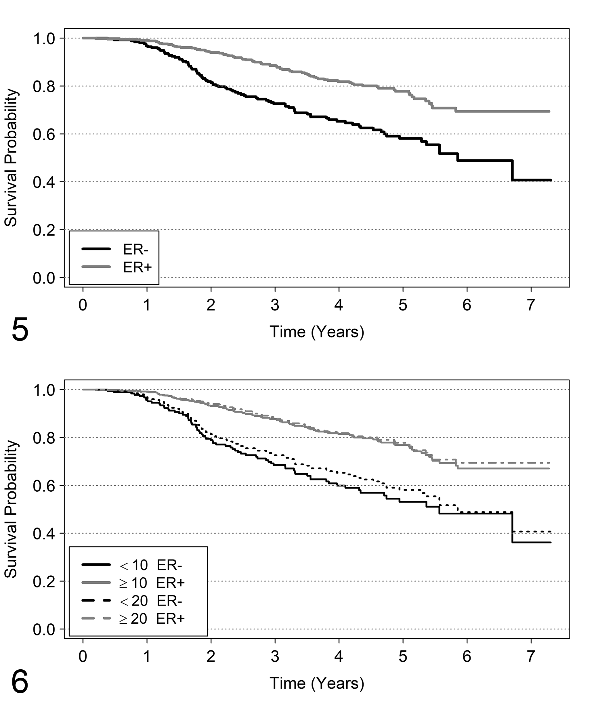
Kaplan-Meier survival curves for estrogen receptor (ER) classes. Figures 5–12 illustrate the analysis provided in the text involving node-positive human breast cancer patients treated with chemotherapy. Survival probability curves estimated by Kaplan-Meier method, according to ER classes. The classes considered are as follows. In Figure 5, ER− if fmol/mg <20, and ER+ if fmol/mg ≥20. Figure 6 shows the comparison of the same curves, in addition to those obtained by the “best cutoff method” (ER− if fmol/mg <10 and ER+ if fmol/mg ≥10).
A cutoff can be found using a data-driven method based the “minimum P-value” rule (defined in literature as “optimal” cutoff; see Hilsenbach and Clark 21 ). In this example, a cutoff sequence starting from 5 to 200 fmol/mg was considered. For each of these cutoffs, a log-rank test for comparing survival curves between subjects with ER below and above the cutoff value was performed. The “optimal” cutoff was identified by ER cutoff for which the minimum P-value was obtained. According to this criterion, the “best” cutoff was 10 fmol/mg (log-rank test = 33.2; P < 0.0001). Although a correction of P-values should be applied to account for the multiplicity of statistical tests, 21 we are not interested to calculate the correct P-values, but only to show how procedures for data-driven selection of cutoff work. Despite the criticism previously illustrated against the categorization of markers measured in continuous scale (see “Inclusion of the Marker in the Analysis”), in this case the results seem to be reproducible, since this cutoff has been previously used (see, eg, Courdi, 8 Nicholson et al, 33 Andersen et al 3 ).
The survival curves obtained by the old and new “best” cutoff are shown in Figure 6. The curves for ER+ patients are superimposable, while there is a difference between the curves of ER− patients classified by the 20 fmol/mg and the 10 fmol/mg cutoffs. In particular, the group of patients with ER <10 fmol/mg show a slightly worse prognosis than the group of patients with ER <20 fmol/mg. To consider ER as a continuous variable, a naïve approach is to fit a Cox model with a linear effect of ER content. The following results were obtained by this approach: hazard ratio = 0.9985, 95% confidence interval (CI) from 0.9972 to 0.9998, P-value = .0281. This result indicates that prognosis improves with the increase of ER fmol concentration. Is this result clinically reasonable? To give an answer, the first step is to examine the distribution of the ER content. The difference between mean and median of ER content (respectively, 96 and 36 fmol/mg) suggests an asymmetrically shaped distribution, which is clear in Figure 7a. The distribution of ER content is heavily asymmetrical and 72% of patients have ER ≤100 fmol/mg. It is likely that a difference of 1 fmol/mg is more clinically relevant when ER has low values than when ER has high values.
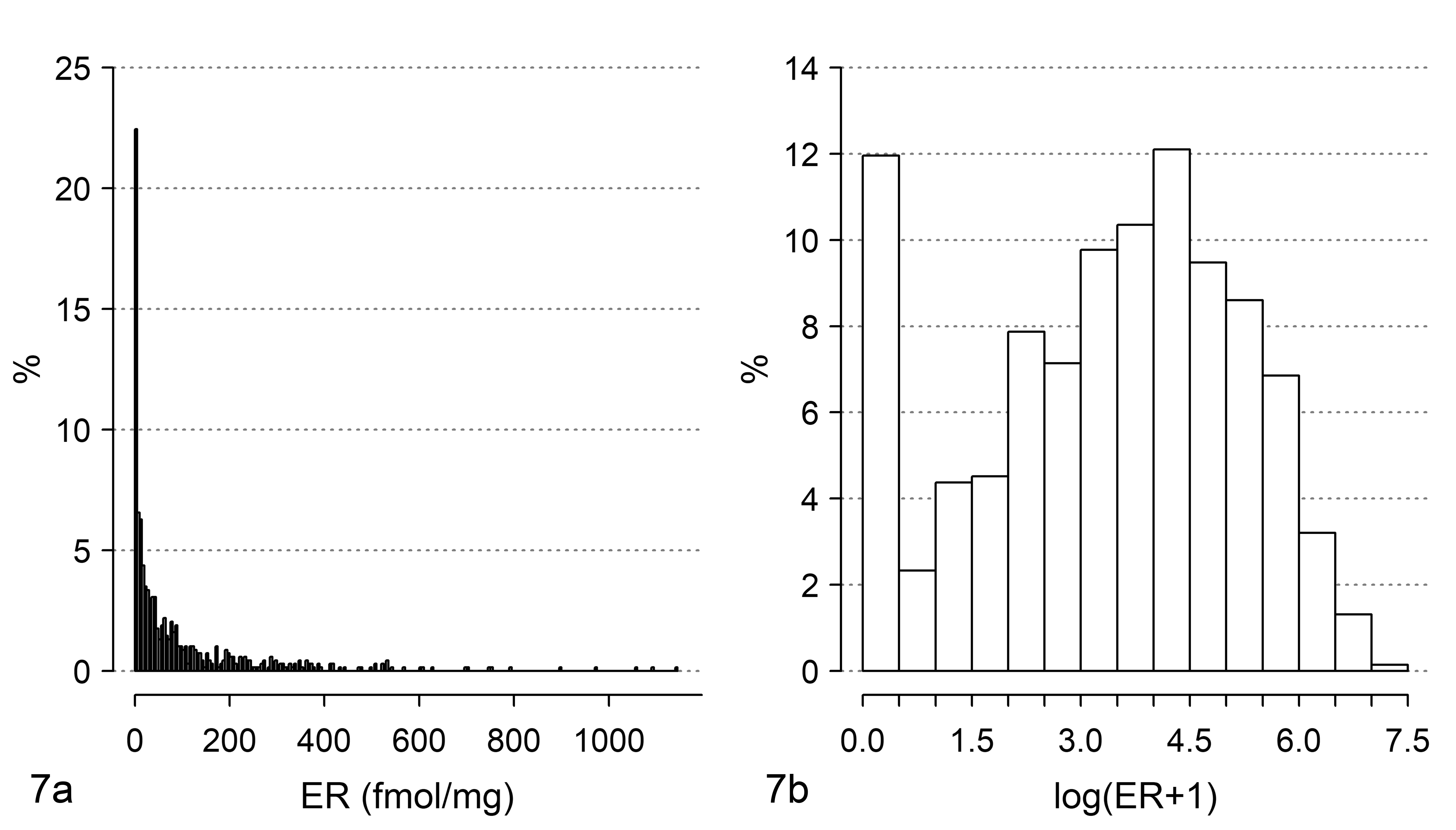
Distribution of estrogen receptor (ER) levels in a sample of tumors from node-positive human breast cancer patients. The same data are shown (a) on the original scale (fmol/mg) and (b) using a log(ER + 1) scale.
In this situation, the application of a data scale transformation should be preferred in order to (1) attribute more weight to small differences in fmol/mg starting from low ER values than to high ER values and (2) reduce the spread of the ER values. A widely diffuse transformation is performed via logarithmic scale. Because the ER content recorded in the dataset is, for some patients, equal to 0 fmol/mg, an empirical solution that can be adopted is log(ER + 1). This scale transformation, which is frequently applied in breast cancer literature (see, eg, Bardou et al, 4 Shek et al 43 ) satisfies both the aforementioned requirements. For requirement (1), as an example the difference of 5 fmol from 5 to 10 in logarithmic scale is Log(10) − Log(5) = 0.693 and from 100 to 105 is Log(105) − Log(100) = 0.049. For the second requirement, see Figure 7b. Furthermore, some authors (eg, Harrell et al 18 ) highlight that in Cox models, often complex prognostic relationships could be satisfactorily approximated using a simple transformation of the explanatory variable, such as the logarithm.
The prognostic relationship is now evaluated by including ER in log scale (LER) into the Cox model (linear relationship). We obtained the following: hazard ratio = 0.81, 95% CI 0.75 to 0.87 (P-value < .0001). These results indicate that for each increase of 1 unit LER, the ratio between hazard of death for LER = x and the hazard of death for LER = x + 1 is estimated to be 0.81 and does not change for each value of LER. Thus, for example, the ratio between the hazard of death for LER = 0.69 (about 1 fmol/mg) and LER = 1.69 (about 4 fmol/mg) is 0.81 and the ratio between the hazard of death for LER = 2.40 (about 10 fmol/mg) and LER = 3.40 (about 29 fmol/mg) is 0.81, and so on. To facilitate the evaluation of model results, it is preferred to represent the estimated hazard ratios in the original measurement scale by considering as reference the lowest ER value. In Figure 8, the shape of the ratio between hazard of death for each ER fmol/mg value and the hazard of death for 0 fmol/mg can be observed. The decrease in hazard ratio is steeper for low ER values than for higher ones. For example, the hazard ratio of death from 0 to 10 fmol/mg is 0.52, from 0 to 20 fmol/mg is 0.45, from 0 to 50 fmol/mg is 0.37 and from 0 to 100 fmol/mg is 0.32.
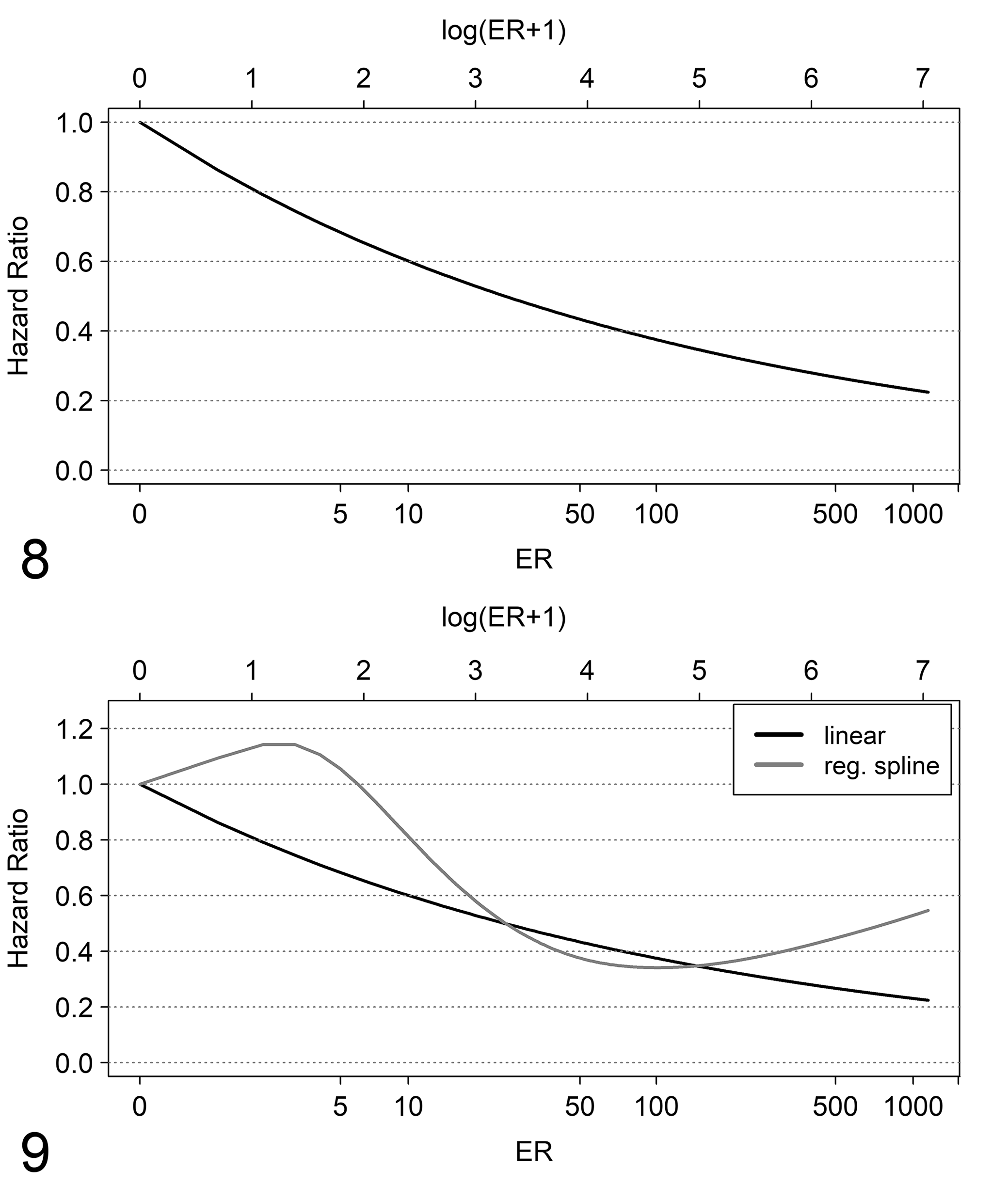
Shape of the hazard ratio of death.
A relevant issue to be discussed is how much a researcher is confident with the linear relationship. When the linear relationship seems to be too “restrictive,” the possible existence of a more flexible relationship needs to be investigated, for example, by including into the Cox model power functions of LER, such as polynomials or fractional polynomials 40 or spline functions. 17,20 As a matter of fact, after including cubic spline functions, a more complex functional relationship than a linear one was found. The comparison of model predictions with spline (restricted cubic spline with 4 knots 17 ) and model predictions with a linear relationship is shown in Figure 9. There may be noted a slight increase of the hazard ratio from 0 to 2 fmol/mg and after 200 fmol/mg for the model with spline function, whereas for the model with a linear relationship the hazard ratio always decreases with the increasing of fmol/mg. To compare the 2 models mentioned above, we used the likelihood ratio test, with null hypothesis that the contribution of the nonlinear terms is null. Results are the following: χ2 = 7.2958 with 2 degrees of freedom, and P-value = .02605; therefore, the second model seems to be better. However, a statistically significant test cannot be used as the only criterion to choose which model better represents the prognostic behavior; thus, the more complex model can be preferred over the simplest one only if the shape of the hazard shown in Figure 9 has a credible clinical/biological explanation.
If the aim is to predict the outcome, the discriminant ability of the two models (AUROC) should be considered. First, the measure by Harrell’s c statistic for the AUROC on the whole follow-up is equal to 0.634 for the model with linear relationship and to 0.633 for the model with spline functions. The 2 models provide very similar discriminant ability (ie, about 63% of patients who have longer survival times have higher ER values than patients who have shorter survival times). Thus, according to this perspective it seems useless to choose the more complex model. More detailed information can be obtained by dynamic ROC curves which provide cumulative AUROCs for prespecified follow-up times. This allows investigation of the possible time in which to assess the patients for the better model discriminant ability. The dynamic ROC curves for the linear and spline Cox regression models are reported in Figure 10. Subdividing the follow-up time into 180-day intervals, the highest AUROC value is 0.72 at 180 days for the model with spline function, and is 0.70 at 360 days for the model with a linear relationship. These results may suggest that ER content shows a better discriminant ability at short follow-up times. After 900 days, the discriminant ability of the model with spline function is slightly better than that of the model with a linear relationship. The highest discriminant ability of ER when considered as dichotomous (cutoff: 20 fmol) is at 360 days, with AUROC = 0.65. This value is lower than the AUROC obtained when ER is considered in a continuous scale (LER).
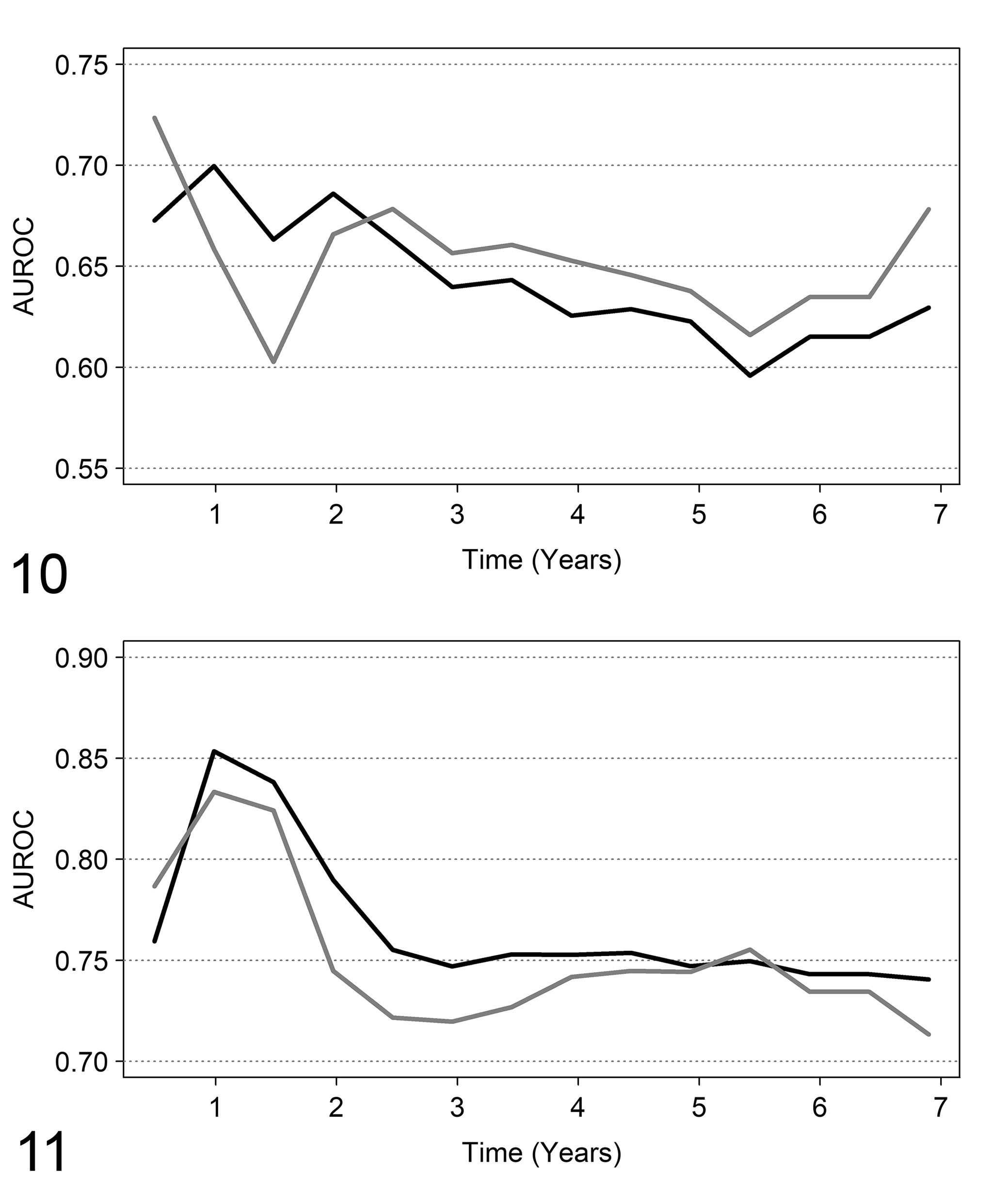
Discriminant ability by dynamic ROC curves. On the X axis, the follow-up time. On the Y axis, the area under the ROC curve (AUROC) estimated by dynamic ROC curve methods.
Multivariable analysis of ER content and time to death
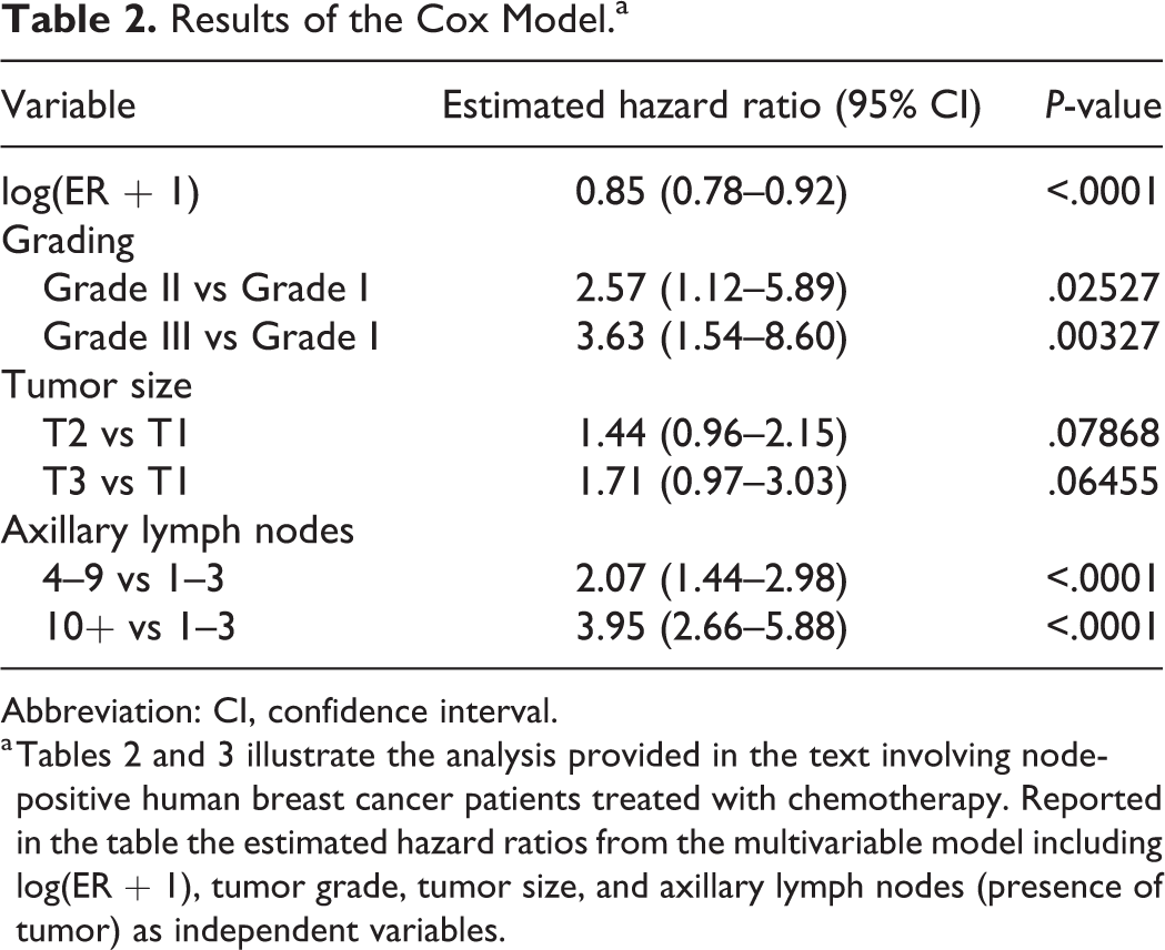
The first model to be considered includes tumor size, tumor grade, number of axillary lymph nodes with detected tumor, and LER (ie, log(ER + 1)). The LER scale was considered for the same reasons discussed in the previous section. The results are reported in Table 2. When the joint prognostic effect of the variables is considered, the statistically significant prognostic factors are ER content, tumor grade, and number of affected axillary lymph nodes, but not tumor size. The three pathological variables are categorical (each one having three classes) and have to be included in the Cox model as “dummy variables”; typically, such variables assume only the values 0 and 1. For a categorical variable with three classes, two dummy variables are needed. One of the classes is chosen as the reference and the Cox model estimates the ratio between the hazard of death of each of the two remaining categories and the hazard of death of the reference one. For example, the chosen reference category for tumor grade is grade I; thus, the hazard of death for patients with grade II is 2.57 times the hazard of death for patients with grade I, and the hazard of death for patients with grade III is 3.63 times the hazard of death for grade I patients. The corresponding P-values (Table 2) test the null hypothesis that the hazard ratio is equal to 1, that is, no difference between the hazard of death for Grading II (or III) and grading I. Both hazard ratios are significantly different from 1. This is in agreement with a significant prognostic effect. Similar results are shown for involvement of axillary lymph nodes but not for tumor size.
Results of the Cox Model.a
Abbreviation: CI, confidence interval.
a Tables 2 and 3 illustrate the analysis provided in the text involving node-positive human breast cancer patients treated with chemotherapy. Reported in the table the estimated hazard ratios from the multivariable model including log(ER + 1), tumor grade, tumor size, and axillary lymph nodes (presence of tumor) as independent variables.
Together with the P-values, 95% confidence intervals provide relevant information about the values of the hazard ratio that we would find if the whole population of patients was examined. For example, if the whole population of node-positive breast cancer patients receiving the same chemotherapy were examined and patients with Grade III tumors were compared with patients with Grade I tumors, the hazard ratio of death is expected (with a probability of 0.95) to lie between 1.54 and 8.60.
In the previous analysis, LER was included as linear effect. Is there evidence in multivariable analysis for a more complex relationship? The inclusion of splines does not suggest any improvement over the previous model. We performed a likelihood ratio test for comparing a model with a spline function with 4 knots and the model with only the linear relationship of LER, the result was the following: χ2 = 3.4669 with 2 degrees of freedom, and P-value = 0.1767. This can be interpreted as follows: after the adjustment for the other known prognostic factor, the complex relationship is no longer statistically significant. This is one motivation for evaluating the marker by multivariable analysis, together with the other prognostic factors that are likely associated with the marker itself.
Concerning the discriminant ability, the Harrell’s c statistic was equal to 0.73 for the multivariable model. For marker evaluation, the main question is: does ER content improve the discriminant ability when added to the other variables? Harrell’s c statistic for the model with all the prognostic variables except ER is 0.71. Thus, it seems that the contribution of ER content to the discriminant ability of the three prognostic factors is limited. Because in univariate analysis (previous section), ER showed a better discriminant ability at early follow-up times, this evaluation was performed also in the multivariable analysis. Again, the highest discriminant ability was found at early follow-up times: 360 days (Fig. 11), and the model with ER slightly outperforms the model without the variable (AUROC = 0.85 vs AUROC = 0.83).
The improvement in discriminant ability obtained by including ER content (in logarithmic scale) in the model can be evaluated by the integrated discriminant index (IDI), which at 360 days is 0.0026. This value is close to zero indicating a low discriminating improvement. From the hypothesis test for evaluating the marker’s contribution (null hypothesis: IDI = 0), the P-value was 0.359; thus, there is no evidence of a discriminant improvement in prognosis given by ER (in this type of chemotherapy-treated patients) when grade, tumor size, and number of axillary lymph nodes are jointly considered along with the marker. When ER is considered as dichotomous (cutoff 20 fmol/mg) the highest discriminant ability is again at 360 days and AUC is 0.84, slightly lower than AUROC for the model with ER on continuous logarithmic scale.
Analysis of Impact of ER on Tumor Recurrence
In this section, we assess the impact of ER on tumor recurrence. As discussed in the first part of the commentary, this endpoint requires methods for analysis of competing risks: death without relapse is a competing event that would prevent observation of the event of interest.
Univariate analysis of ER and tumor recurrence
In the current example, among 171 patients who were dead, 21 had not experienced tumor recurrence. The probability of concern is the cumulative probability of tumor recurrence as the first event, that is, the crude cumulative incidence. The estimates of the crude cumulative incidences are shown in Figure 12; in the figure we reported also the naïve estimates obtained by the Kaplan-Meier method. First, let us consider ER as a categorical variable by setting the cutoff to 20 fmol/mg. In Figure 12, the patterns of the cumulative incidence obtained by the two methods are similar and slight differences are evident only at follow-up times greater than 1500 days. This result is expected in this case, because of the low number of patients who died without tumor recurrence. In other situations, where a higher number of competing events is observed, more substantial differences between the two estimates are expected. Furthermore, the two estimates are nevertheless interchangeable. The naïve Kaplan-Meier estimate is a biased estimate of the probability of recurrence given the “removal” of death without recurrence, that is, the cumulative probability of recurrence if this could be observed for all patients. On the contrary, the crude cumulative incidence estimator is the unbiased estimate of the cumulative probability of recurrence observed as the first event.
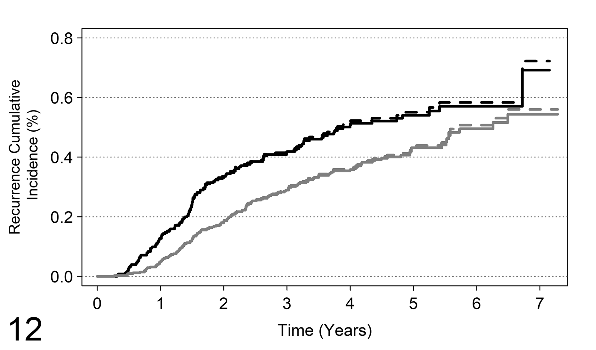
Analysis of competing risks for tumor recurrence, where the competing event is death as the first occurred event. The figure reports the cumulative incidence curves of tumor recurrence for ER (ER− if fmol <20 and ER+ if fmol ≥20). Solid lines: crude cumulative estimates; dashed lines: naïve Kaplan-Meier estimates. Black lines: ER−; gray lines: ER+.
Concerning the comparison between crude cumulative incidences of recurrence for patients with ER− and ER+ status, a significant difference was found (Gray test = 12.97, P-value = 0.0003); thus, a higher incidence of recurrence is expected in ER− patients.
To find the data-driven “optimal” cutoff, ER was dichotomized by a cutoff sequence starting from 5 to 200 fmol and the cutoff corresponding to a minimum P-value was chosen. According to this criterion, the “best” cutoff was 9 fmol/mg (P-value of Gray test <.0001).
Multivariable analysis of ER and tumor recurrence
The analysis was performed by estimation of 2 models: the Fine and Gray regression model for competing risks and, for comparison purposes, the Cox model for recurrence times, in which times to death without tumor recurrence are censored. The results are reported in Table 3. Despite the slight differences among hazard ratios (again, this result was expected because of the low number of deaths without recurrence) the interpretation of the results of the two models is different. Both models account for the presence of competing risks but from a different perspective. For the Fine and Gray regression model, if the (subdistribution) hazard ratio is significantly different from 1, then the crude cumulative incidences (eg, between Grade III and Grade I; see Table 3) are different. This relationship cannot be extended to the Cox model, because the hazard ratio from the Cox model (which is a ratio between cause-specific hazards) does not have a direct relationship with crude cumulative incidences.
Results of Multivariable Analysis.a
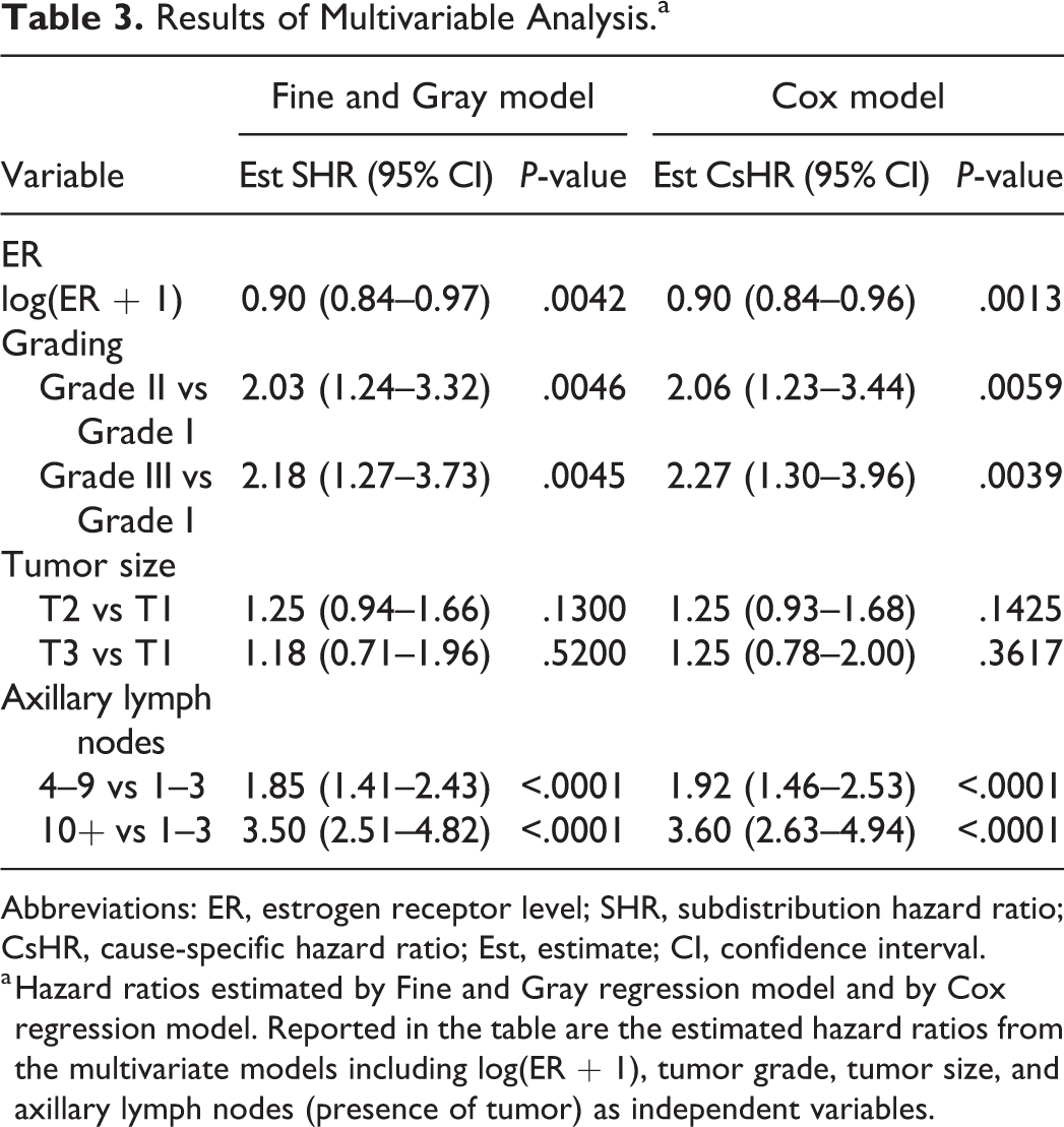
Abbreviations: ER, estrogen receptor level; SHR, subdistribution hazard ratio; CsHR, cause-specific hazard ratio; Est, estimate; CI, confidence interval.
a Hazard ratios estimated by Fine and Gray regression model and by Cox regression model. Reported in the table are the estimated hazard ratios from the multivariate models including log(ER + 1), tumor grade, tumor size, and axillary lymph nodes (presence of tumor) as independent variables.
From the estimates of hazard ratios, a significant impact of estrogen receptor levels (included in log scale) emerged, with an estimated hazard ratio of 0.90 (95% CI 0.84–0.97). This result suggests that the hazard of tumor recurrence decreases with increased levels of ER, and consequently the crude incidence of recurrence is lower in subjects with higher ER levels.
Discussion
This commentary illustrates, by using data from a cancer trial on humans, some of the most appropriate statistical approaches to analyze the prognostic significance of novel tumor markers that could be applied also to a novel histopathological variable measured on continuous scale, or to any new prognostic variable.
The necessity to plan in advance a statistical approach tailored to the clinical study was stressed and insights were provided on study planning, to recognize the existing link between study aims, statistical models, and adequate sample size. According to this, before starting the study on a new prognostic variable, oncologists and clinicians in general should consider the correct specification of the endpoint, the best-suited survival model for the endpoint, the measurement scale of the new prognostic variable, and the statistical methods aimed at quantifying the prognostic/predictive information provided by the variable in terms of statistical significance and/or in terms of discriminant ability.
From our professional experience, most of the problems that are spotted by a statistician when consulted after the end of a study are the following:
– lack of representativeness of the sample with respect to a wider population of subjects sharing the same lesions, due to an inadequate sampling plan;
– data retrieved from medical records (retrospective studies) with insufficient quality of data to satisfy the aims of the study;
– inadequately small sample size for the aim of investigating the prognostic value of the variables under examination;
– an empirical choice of cutoffs for numerical markers without investigation of the marker on the original measurement scale;
– inadequate statistical methods of analysis that strongly reduce the reliability of results;
– a blind interpretation of P-values that makes statistical significance prevail over the most important clinical relevance;
– lack of evaluation of the discriminant ability when the statistical model is used as an aid to clinical decision making.
The evaluation of prognostic/predictive tumor markers or histopathological variables is challenging and should aim toward a personalized medicine framework, intended to improve clinical decision making. Because of the potentially relevant role of a marker, the statistical analysis should yield reliable results. For this purpose, the endpoint has to be clearly defined and its choice depends on the study aim; according to the aim, an endpoint can be “patient oriented” or “tumor oriented.” The most used patient-oriented endpoints are the patient’s overall survival or quality of life. Tumor-oriented endpoints generally relate to the response of the tumor to therapeutic strategies, and different tumor-oriented endpoints include local relapse, distant metastases, or contralateral tumors. Since each one of the above-mentioned endpoints provides different information on the disease course, it is usual and highly recommended to plan the study by considering both patient-oriented and tumor-oriented endpoints. The latter are only a subset of the events which can be observed and should be planned to consider the presence of competing risks.
When the goal is to evaluate the prognostic/predictive role of a marker or histopathological variable, a multivariable analysis is the adequate strategy. The analysis should include all of the previously well-known clinical and pathological variables (prognostic or predictive), in order to quantify the added contribution provided by the new variable and to allow clinicians to decide whether to include the new marker (or histopathological variable) in their routine practice based on the costs and benefits. Statistical significance from a single study is not a sufficient basis for making clinical decisions, and the discriminant ability should also be provided. Where possible, meta-analyses should be considered to take into account the results of different studies. However, the majority of meta-analyses include only a measure of covariate effect, such as the hazard ratio. This is not a measure of discriminant ability; therefore, meta-analysis using the discriminant ability should be preferred. An example is provided by Van den Boorn et al. 45
When statistical significance is of concern, the required sample size should be defined according to a minimal clinically relevant prognostic effect size. However, the sample size (number of events and of patients) could be large if a small effect size is to be detected. Furthermore, when a multivariable analysis is planned, the required sample size could be even larger: in fact, the more variables that need to be included, the larger should be the sample size. Methodological papers showed that at least 10 events for each variable should be considered to obtain reliable model results. 7,44 As a consequence, when a low number of events are expected to occur for the disease of interest (eg, low incidence of tumor recurrence or deaths) the adequate sample size may need to be very large and, thus, difficult to reach by a single research center.
A topic that has not been discussed in this commentary concerns the procedures that are aimed to achieve a generalizable result, such as, for example, the building of prognostic scores using model results. To achieve this goal, model selection should be based on validation procedures both internal (eg, cross-validation) and external to calibrate the score. This is of uttermost importance but it was not possible to discuss this topic here.
The authors believe that the role of each study is to contribute to improving the scientific background, and to this aim, a study should be correctly conducted not only including the experimental components (clinical, biological, pathological) but also with the application of the best-suited and appropriate statistical analysis. The role of the variables on the disease course is often complex, but it seems that most researchers fail to realize that unreliable results could be obtained by the application of a too simplified statistical approach, adopted by honest researchers who are not sufficiently experienced in statistical method selection. On the other hand, statisticians who are not experienced in medicine could apply complex statistical methods that are inadequate to the study aims. In conclusion, the best strategy to obtain sound and reliable results is to work in close collaboration, with each discipline providing the study with its expertise, and learning how to communicate effectively to explain technical issues by using terms and practical examples that can be understood by each member of the team. We hope that this commentary and the included examples will facilitate communication and the cooperation among biostatisticians, oncologists, and pathologists.
Supplemental Material
Supplemental Material, sj-pdf-1-vet-10.1177_03009858211014174 - Kaplan-Meier Curves, Cox Model, and P-Values Are Not Enough for the Prognostic Evaluation of Tumor Markers: Statistical Suggestions for a More Comprehensive Approach
Supplemental Material, sj-pdf-1-vet-10.1177_03009858211014174 for Kaplan-Meier Curves, Cox Model, and P-Values Are Not Enough for the Prognostic Evaluation of Tumor Markers: Statistical Suggestions for a More Comprehensive Approach by Patrizia Boracchi, Paola Roccabianca, Giancarlo Avallone and Giuseppe Marano in Veterinary Pathology
Footnotes
Declaration of Conflicting Interests
The author(s) declared no potential conflicts of interest with respect to the research, authorship, and/or publication of this article.
Funding
The author(s) received no financial support for the research, authorship, and/or publication of this article.
Supplemental material for this article is available online.
References
Supplementary Material
Please find the following supplemental material available below.
For Open Access articles published under a Creative Commons License, all supplemental material carries the same license as the article it is associated with.
For non-Open Access articles published, all supplemental material carries a non-exclusive license, and permission requests for re-use of supplemental material or any part of supplemental material shall be sent directly to the copyright owner as specified in the copyright notice associated with the article.