
Abstract
High-throughput, genome-wide transcriptome analysis is now commonly used in all fields of life science research and is on the cusp of medical and veterinary diagnostic application. Transcriptomic methods such as microarrays and next-generation sequencing generate enormous amounts of data. The pathogenetic expertise acquired from understanding of general pathology provides veterinary pathologists with a profound background, which is essential in translating transcriptomic data into meaningful biological knowledge, thereby leading to a better understanding of underlying disease mechanisms. The scientific literature concerning high-throughput data-mining techniques usually addresses mathematicians or computer scientists as the target audience. In contrast, the present review provides the reader with a clear and systematic basis from a veterinary pathologist’s perspective. Therefore, the aims are (1) to introduce the reader to the necessary methodological background; (2) to introduce the sequential steps commonly performed in a microarray analysis including quality control, annotation, normalization, selection of differentially expressed genes, clustering, gene ontology and pathway analysis, analysis of manually selected genes, and biomarker discovery; and (3) to provide references to publically available and user-friendly software suites. In summary, the data analysis methods presented within this review will enable veterinary pathologists to analyze high-throughput transcriptome data obtained from their own experiments, supplemental data that accompany scientific publications, or public repositories in order to obtain a more in-depth insight into underlying disease mechanisms.
Keywords
Life science research, including molecular mechanisms of pathological processes, has been massively influenced during the past decade by the advent of microarray-based gene expression techniques, also referred to as transcriptomics. 132 The transcriptome represents the set of all ribonucleic acid (RNA) molecules, including messenger RNA (mRNA), ribosomal RNA (rRNA), transfer RNA (tRNA), and other noncoding RNA transcribed in a cell or tissue at a certain time point. The interpretation of common gene expression experiments at the level of the RNA transcripts is based on the assumption of a positive correlation of the amount of mRNA and protein, as inferred from the central dogma of molecular biology, 29,119 no matter if either microarray systems or alternative methods such as next-generation sequencing systems, reverse transcription quantitative polymerase chain reaction (RT-qPCR), or northern blots are used. However, the relationship of mRNA to protein and phenotype is not a simple linear function but underlies a complex regulatory network and is influenced by various posttranscriptional and posttranslational processing and modification processes. 31 A prominent example is tumor protein 53. The encoded protein possesses manifold important regulatory functions during cell cycle, apoptosis, and tumorigenesis. The activity is mainly controlled through posttranscriptional and posttranslational modification, and at least 12 different isoforms with diverse function are known. Thus, direct transfer from mRNA level to protein level is not applicable. 82,180 In general, posttranscriptional regulatory processes, the different half-lives of proteins, but also technical shortcomings are reported to be responsible for a poor correlation between mRNA and protein levels. 55 Literature reports concerning the relationship of mRNA and protein content are quite variable and find correlation coefficients in the range from 0.36 to 0.76. 56,95,99 Notably, stochastic effects and intrinsic noise preclude detection of the inherent relationship in experiments dealing with low absolute molecule numbers such as single cell analysis, whereas the correlation is rather strong employing larger populations of cells or tissues and large-scale methods such as transcriptomics and proteomics. 119 A study reports that 67% of the variance in protein amount can be explained by the variance in mRNA amount and further subdivides the explained variance into effects of the coding sequence (31%), absolute mRNA amount (27%), structure of the 3′ untranslated region (8%), and structure of the 5′ untranslated region (1%). 162 Even if no direct linear correlation between the protein to gene level exists, mRNA-based gene expression methods such as microarrays enable researchers to unravel physiological or pathological processes currently active within a cell or tissue.
Microarray technology matured in the 1990s and has revolutionized modern human and veterinary pathology research. 120 The goals of microarray studies in veterinary medicine are to identify diagnostic markers, therapeutic targets, or important factors for understanding the biology of the disease. 64 Nonetheless, histologic evaluation of formalin-fixed, paraffin embedded tissue (FFPE) samples doubtlessly remains the diagnostic standard in anatomic pathology. Thus, for an envisioned microarray experiment with a veterinary pathology background, it is highly recommended to simultaneously collect FFPE material to morphologically validate the results gained by microarray analysis. Moreover, histologic quality assurance, classification, and sample selection are key to a successful microarray experiment, since a heterogeneous histologic presentation of tissue samples will certainly be mirrored by more heterogeneous molecular differences. 64
Enormous efforts have been undertaken to standardize the presentation and exchange of microarray data. In fact, good scientific practice requires deposition of raw and processed data in accordance to minimum information about microarray experiment standards defined by Brazma et al. in public archives. 10,18 Consequently, a vast amount of microarray gene expression data sets are available through public repositories such as Gene Expression Omnibus (GEO) by the National Center for Biotechnology Information (NCBI) 10 and ArrayExpress by the European Bioinformatics Institute, 133 offering an easily accessible opportunity for reanalysis and combination of these previously published data. Supplemental Table S1 comprises a selection of freely accessible transcriptome data sets deposited within the ArrayExpress database, which are of special relevance for veterinary pathology. However, to explore the extraordinary potential of these data, a basic knowledge of possible methods and applications is crucial. The present review thus aims to provide the reader with a clear and systematic basis from the point of view of a veterinary pathologist.
Various freely available software tools for microarray analysis have been developed under the Bioconductor project in the R statistical computing project and programming language environment, requiring basic programming skills. 48 However, profound knowledge in large-scale biomathematics and computational analytics is not a main constituent of the specialization of a veterinary pathologist. Hence, this review especially focuses on data analysis techniques available for users without programming skills and describes appropriate methods for specific research purposes from a pathologist’s point of view. A main goal is to assist the reader in the transformation of the huge amount of information, obtained by a single experiment, into biological knowledge and to point out important challenges and pitfalls by presenting representative data that illustrate common problems in data analysis. Important to emphasize, all algorithms beyond low-level analysis discussed in this review are applicable universally to all data sets regardless of the platform used.
Moreover, as the next-generation sequencing platform RNAseq is considered to continuously replace microarray technology, this review additionally dedicates a section to the introduction of this emerging technology. Although this technology will with further maturation potentially replace microarray analyses, it should be emphasized that microarray analysis still represents the most validated, sensitive, reliable, and robust method with matured, user-friendly, and partly freely available processing and analysis software.
Experimental Design and Microarray Hybridization
Experimental Design
Careful planning of the experimental design of a microarray experiment represents the most crucial step in identifying true and biologically relevant differences in the output data. No statistical algorithm is able to rectify shortcomings in the experimental setup. Therefore, it is extremely important to carefully choose a design that is able to control systemic factors and that is minimally influenced by external sources. 1,173 Text Box 1 summarizes important considerations for an expedient experimental design.
Important Considerations for an Expedient Experimental Design for Microarray-Based Gene Expression Analysis
Definition of study objectives
Specification of experimental condition
Selection of a measurement platform Study objectives (gene expression, microRNA, splicing variants) Species availability Representation of genes of interest on the array
Measures for reduction of technical and biological variability Definition of biological sampling design Determination of biological and technical replicates
Determination of hybridization design
Microarray experiments produce data on the expression level of thousands of genes. The downside, however, is that the data may be noisy and therefore not as sensitive as other methods, especially for genes with low transcription levels, such as transcription factors. 36,151 Thus, the first question a researcher should ask is whether microarray technique is indeed appropriate for achieving the research objective. Microarray experiments generate relative gene expression data. 24 In case absolute quantitative data and a defined threshold are needed to make the research statement, RT-qPCR 157 or digital PCR 67 using a quantitative standard for calibration is the more appropriate method of choice. 67,157
Selection of the Microarray Platform
One first decision is whether to use a 1-color approach, in which a single sample is hybridized to 1 array, or a 2-color approach, in which 2 samples, labeled with different fluorophores, are competitively hybridized to 1 array. 114 Traditionally, 2-color arrays have been used to reduce the technical bias introduced during microarray production. The increased accuracy and sensitivity of current microarrays relegated the use of 2-color arrays out of the focus to a small percentage. However, the comparison between the 2 approaches shows equivalent performance and high concordance. 9
Although the production of “in house” printed microarrays is an application-oriented customizable method, commercial microarrays ensure consistent high quality and comparability within the experiment and between different experiments and allow easy access to the technology due to standardized work flows. 59 The available platforms differ in probe design, production method, labeling, and hybridization protocols, and exhaustive comparisons between different platforms have been performed in various studies. 9,23,97,175
The main differences between the platforms reside in the probe length and probe deposition technology. In situ photolithography technique directly synthesizes oligonucleotides, usually 25 nucleotides in length, on a glass slide (eg, Affymetrix, Santa Clara, CA, USA). Inkjet printing processes attach oligonucleotides with a length of about 60 nucleotides on a glass slide (eg, Agilent, Santa Clara, CA, USA), and in bead microarray systems, oligonucleotides with a length of about 50 nucleotides are bound to magnetic beads and assembled randomly across the array (eg, Illumina, San Diego, CA, USA). The different length of the oligonucleotides attached to the solid surface results in different hybridization properties. 59 The longer nucleotides are more tolerant to sequence mismatches and have a higher sensitivity but reduced specificity. Generally, 1 probe is able to represent a transcript or gene. 59 If shorter oligonucleotide sequences are used, multiple probes generally represent 1 transcript; this has a positive effect on the signal/noise ratio and broadens the dynamic range of transcript detection. Despite the technical differences, all platforms show comparable low variance between technical replicates and a high overlap in differentially expressed genes (DEGs). 36,92,173 Thus, the choice of the technology is predominantly based on the species availability, study objectives, costs, and personal preferences. Gene expression microarrays for a broad range of vertebrate and nonvertebrate species are commercially available (Supplemental Table S2).
Determination of the Number of Biological Replicates
Biological variability represents the greatest source of variation in microarray experiments, and therefore, the decision to determine the number of biological replicates is one of the most difficult decisions of any experimental design to achieve adequate power and validity for statistical tests. 1 The number of biological replicates to detect meaningful expression changes with the desired statistical power, and an acceptable type I error is dependent on the magnitude of the expected effect and the variability within the population. 69,92,113,115,173 The necessary parameters should be estimated from real data, ideally from a pilot study, and the sufficient sample size thereafter should be calculated using a power analysis adjusted for microarray analysis (http://sph.umd.edu/department/epib/sample-size-and-power-calculations-microarray-studies). 115
A more empirical approach is provided by studies examining the effect of different numbers of biological replications in a variety of available real data sets to detect a level of replication that ensures high confidence and stability of the results. 115 For most studies, a good power and stability could be obtained with fewer than 15 replicates—often fewer than 10. However, fewer than 5 replicates nearly always resulted in poor power and low stability. 69,113 Other studies reported that at least 8 replicates are needed to detect a significant change in expression values (in this study 3-fold) with a power of 0.8. 1 In this regard, it should be considered that companion or farm animals not kept under experimental conditions exhibit a considerably larger biological variability than laboratory animals or cell cultures. 1 Therefore, more replicates might be needed for studies carried out in any outbred population. 24 However, in practice, the number of replicates will often be determined by the availability of samples (eg, from rare disease entities) and the budget. In this regard, pooling of samples is an important subject. Pooling was introduced to reduce costs and to increase the amount of RNA in microarray experiments. Undoubtedly, pooling of samples reduces the variation of individual samples; however, multiple individual sources provide additional information on the variation between the samples, and additional statistical measures can be applied. 76 Pooled samples express average values that do not necessarily mirror the real situation. High signals add more noise than low signals, and therefore, outliers cannot sufficiently be detected. Accordingly, pooling results in irreversible loss of information. 1 It reduces the effects of biological variation, but it does not reduce the biological variation itself. 78 Nonetheless, pooling may be necessary because of limited quantities of RNA.
Specific Considerations for 2-Color Microarray Experiments
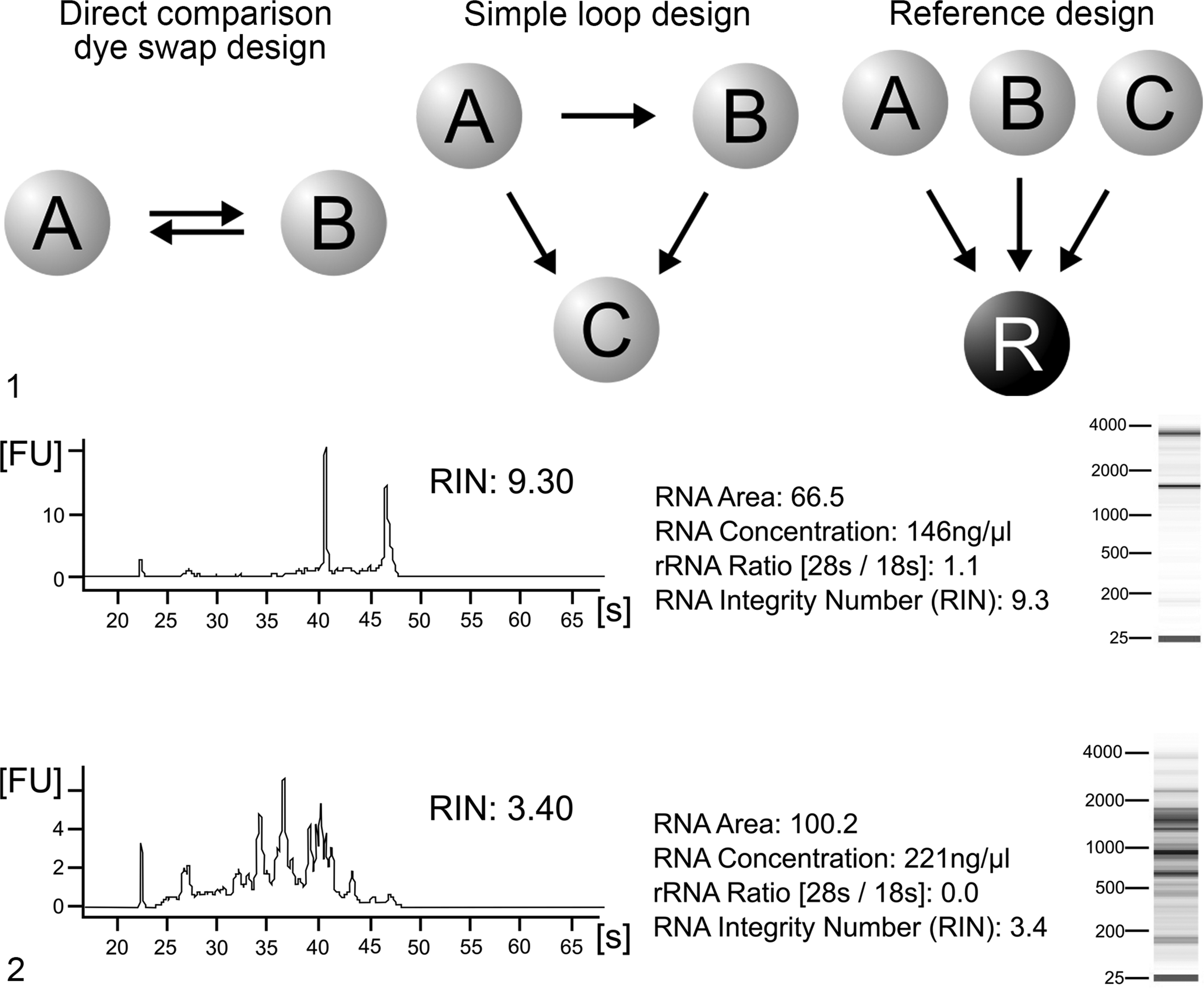
After the number of biological replicates has been determined, the hybridization design for 1-color arrays is straightforward. If a 2-color strategy is chosen, additional considerations on sample combination and dye swap designs should be taken into account (Fig. 1). 78,174 A direct comparison design, in which 2 samples are competitively hybridized on 1 microarray, enables the comparison within the slide and represents a simple and effective design when working with 2 conditions (Fig. 1). For more-factorial analyses, different loop designs were developed (Fig. 1). 34 Particularly important in this regard is that specific statistical methods have to be applied when using complex designs. Therefore, it is always recommended to plan the statistical analysis together with the hybridization design. Reference designs hybridize a common reference with the respective sample on every microarray. These designs are easily extendable and are simpler to analyze than complex loop designs (Fig. 1). 78,174 Dye swap replications are considered to reduce the bias introduced by a higher binding efficiency of certain genes to a specific dye. Their necessity, however, is controversially discussed. 102,150
RNA Isolation and Quality Control
The key to a successful microarray experiment is by far the quality of the initial samples. RNA is a considerably unstable molecule and has a very short half-life, generally of about 30 minutes. 102,150 This is particularly true for tissues with a high concentration of endogenous RNAases such as pancreas, gall bladder, and skin. 102 According to the literature, immediate freezing of small tissue samples (0.1 cm3) in liquid nitrogen gives the best results for subsequent RNA extraction. 102 A feasible alternative is the preservation of tissue with RNA-stabilizing solutions (eg, RNAlater, Qiagen, Hilden, Germany). 169 An additional advantage of an RNA-stabilizing solution treatment is the maintenance of good quality even after repeated freeze-thaw cycles. 137 Since ongoing tissue degradation is detectable in specimens stored at –20°C, most authors recommend storage at –80°C. 137 Others encountered a decreased RNA integrity after a 5-year storage interval and even favor temperatures below –137°C. 102,150 RNA yield and integrity are highly dependent on the composition of the tissue. In general, tissues with a high content of connective tissue not only undergo faster degradation but also result in lower RNA yield. 43,164 Comparing human tissue obtained during autopsy, tissues such as skin or heart showed substantially lower RNA yield than liver, kidney, or lymph node. 164 A prolonged postmortem interval before tissue processing is a particular problem when using tissue from routine necropsy cases in veterinary pathology. Both RNA quality and quantity decrease with increased postmortem interval; however, good-quality specimens can be extracted after a prolonged postmortem interval. 62
Information on RNA extraction methods is summarized in various excellent reviews. 44,102,150 Several studies have also reported novel techniques to extract RNA from formalin-fixed tissue. 28,117 However, formalin fixation causes serious mRNA degradation and a subsequent loss of sensitivity and accuracy. 102 The assessment of RNA quality can be performed by spectrophotometry, fluorimetry, or PCR. 43 Classical denaturating agarose gel electrophoresis assays can be used as well as lab-on-chip technologies (Fig. 2). However, different analyzers have become standard for quality assessment, since they dramatically decrease the amount of RNA needed for the evaluation to the submicrogram scale. Spectrophotometrically, the quality and purity of RNA can be verified on the basis of the ratio of the optical density at a wavelength of 260 nm compared with 240 nm, 280 nm, and 320 nm, respectively. 43 An optical 260/280 ratio greater than 1.8 is usually considered to indicate good quality. 43 Total RNA quality is assessed electrophoretically on the basis of 28S/18 S ratio. Because degradation shifts the ratio toward smaller fragments, a decreased ratio is indicative of degradation. An electropherogram of good RNA quality shows 2 clear peaks for 28 S and 18 s ribosomal subunits (Fig. 2). A 28S/18 S ratio of 1.8 to 2.2 is regarded as perfect quality, but in practice, especially in clinical samples, these values are hard to obtain. 164
RNA Amplification, Labeling, Hybridization and Microarray Washing, Staining, and Scanning
The amount of total RNA necessary for a single labeling reaction is generally about 10 to 40 μg. 116 However, different methods were introduced to amplify small quantities of RNA to study the transcriptome with very limited amounts of input RNA, for instance, derived from biopsies, fine-needle aspirations, or laser capture microdissection. However, it should be emphasized that all amplification procedures introduce a certain bias, as RNA products may be over- or underrepresented in the amplified RNA. 37 For a detailed overview of RNA amplification methods and commercially available amplification kits, see Peano et al. 116 After the RNA samples pass the initial quality control, the labeling process is initiated. However, different labeling protocols have been optimized for specific samples and technologies. Therefore, it is recommended to consult the technical documentation of the respective microarray supplier. Finally, no matter which protocol has been used, the labeled cRNA is hybridized to the microarray. The hybridization is followed by a series of washing and staining steps and subsequently the chip is scanned. 1
Low-Level Analysis
Quality Control of Microarray Data
Data quality assessment is a compelling step to retrieve valuable information from the enormous amount of data generated. The inclusion of arrays with insufficient quality leads to difficulties in the subsequent analysis and introduces a high error rate. 35,60 Thus, any array that does not meet the quality standards should be discarded. 60 In general, quality control measures have to be evaluated on a case-by-case basis and may be more stringent in homogeneous cell-line experiments than in heterogeneous animal experiments. 36,60 The quality of a microarray experiment is evaluated on array level and experiment level. The image obtained from fluorescent scanning is typically processed using a platform-specific software for image processing and intensity extraction. Although this step is an automated process for most commercial platforms image visualization and manual control of grid alignment, control spots and spike in controls is absolutely recommended for the quality assurance on the array level. Quality assessment on the experimental level is used to identify outliers or batch effects within the data set. Supplemental Table S3 summarizes freely available tools for quality control. All quality assessment software tools provide different exploratory graphics or quantitative indices, which facilitate the detection of individual arrays that differ from the other arrays in the experiment (Supplemental Figs. S1–S6). All of these measures are based on the assumption that most genes are unchanged. Accordingly, the scale and the course of the plots should be comparable between the arrays. 60 The effect of low-level analysis can be studied by comparing the results before and after low-level analysis. Small divergences are usually sufficiently compensated by low-level analysis. If low-level analysis cannot remove discrepancies, it is recommended to discard the respective outliers from the analysis. 60 As a general rule, it is recommended to perform the analysis with and without the suspicious sample and compare the results if one array looks suspicious in terms of its quality. Often, it is possible to evaluate the impact of the outlier based on these results. 60
Low-Level Analysis
The aim of the low-level analysis is to improve the comparability of the individual arrays in a microarray experiment by reducing unspecific noise or low-quality measurements to allow the direct comparison of individual transcripts on the different arrays. Raw fluorescent intensity signals are affected by a number of nonbiological sources of variation. 85,143 Artifacts, experimental bias, or random fluctuation can be significantly larger than the biological signals of interest themselves. 85,143 Accordingly, the data have to pass through numerous steps of computational preprocessing, called low-level analysis, to infer meaningful biological data from the measured raw intensity signals. 85
Here, it should be pointed out that the literature causes significant confusion by an ambiguity in the terminology of the low-level analysis step. The terms low-level analysis, preprocessing, and normalization are often used synonymously for the process of calculating comparable expression values out of raw intensity values. In general, preprocessing is a universal term referring to all data-processing and -transformation methods preceding the receipt of expression values. The term thus also includes low-level analysis. The computation of a comparative expression values for every transcript from raw intensity values is defined as “low-level analysis” and, depending on the technology involves different steps, including normalization across an individual microarray (background correction) or across multiple microarrays (normalization). 14,36,143 The term normalization itself, however, should exclusively be used for the reduction of nonbiological chip-specific variation across all microarray chips in an experiment. 36
Commercial microarray suppliers provide their own proprietary low-level analysis algorithms. However, researchers introduced various alternative algorithms to improve the output of this analysis step for special data structures. Unfortunately, a definition of a gold standard for this step is not possible; the most appropriate method depends on various factors, including the biological problem, the nature of the data, and the microarray platform used. 14 Numerous studies have compared different low-level analysis algorithms. 15,105,177 Freely available software applications for this step are listed in Supplemental Table S3.
Following low-level analysis, it is recommended to transform the data from linear scale to a logarithmic scale. Traditionally, a log2-transformation is used. Log-transformation generates an almost normal distribution and facilitates the interpretation of the intensity values by eliminating misleading disproportion between 2 relative changes. 47,143 However, it should be noted that log-transformation has its limitations in the representation of low expression values. 47
Annotation of Microarray Data
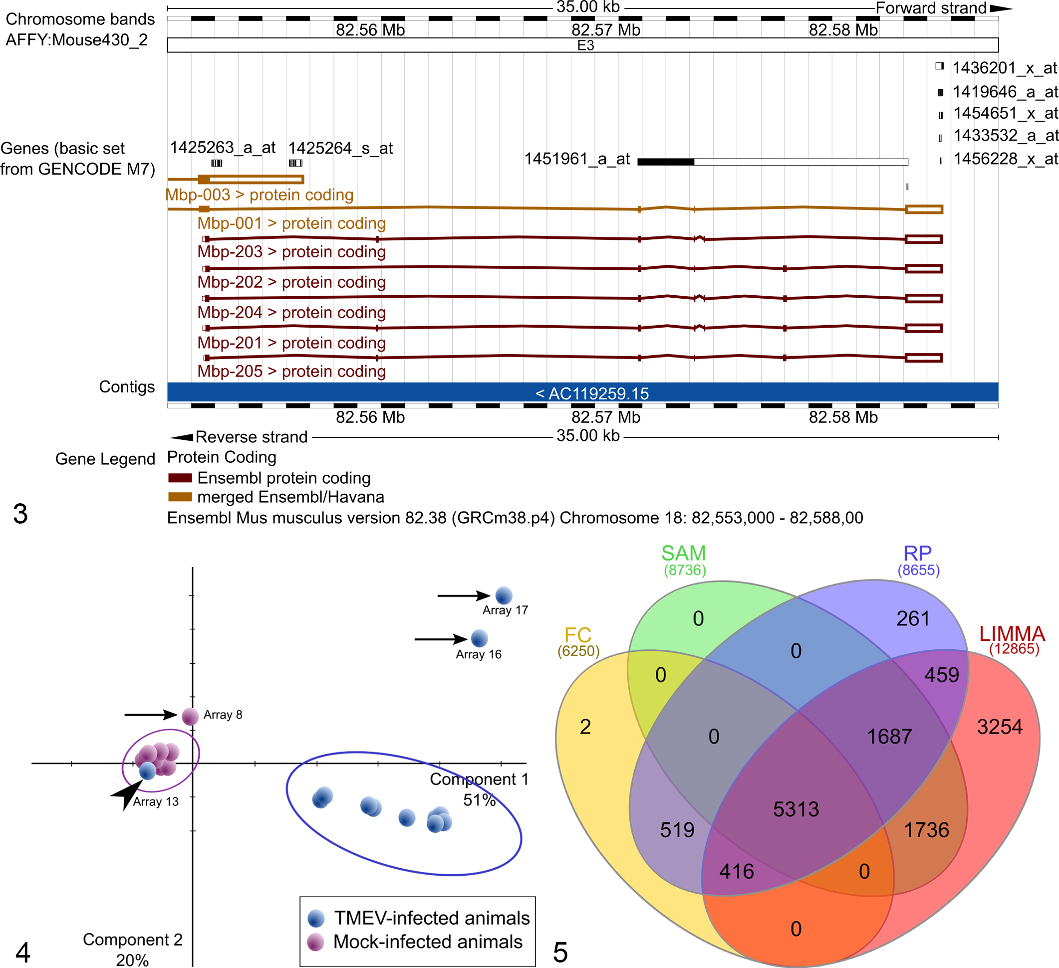
Despite the fact that mRNA is detected in microarray experiments, the results of a microarray study are generally reported on the gene level. 176 Annotation files with different identifiers can be downloaded from the microarray’s supplier webpages and are updated regularly. Since the sequence databases are developing very quickly, it is always recommended to work with the most recent annotation. 98 Therefore, it is good scientific practice to report the database version used in presentations and manuscripts. 104 The transformation from probe level to gene level may not imply a great effort, if each gene is represented by 1 probe. However, if working with oligonucleotide microarrays, in which a single gene is represented by multiple short oligonucleotide sequences (eg, Affymetrix), the transformation may become challenging, especially if multiple probe sets represent 1 gene and show conflicting expression measurements. 40,70 This may be a result of cross-hybridization or different splice variants of a specific gene. 40,70 The position of the target regions of the various probes for each gene can be retrieved and compared using the Ensembl genome browser, as exemplified using the Myelin basic protein (Mbp) gene locus in Fig. 3 and Supplemental Table S4. 22,159 The exact position of the target regions of each of the probe sets is probably the best way to select the single best-performing probe set per gene. For technical reasons, it is typical for 3′IVT microarrays that the probes are concentrated at the 3′ end of the mRNAs and commonly do not cover all possible splice variants. Therefore, if detailed splice variant–specific information is necessary for the scientific hypothesis, whole transcriptome or exon-tiling microarrays or specifically designed RT-qPCRs are the method of choice. 161 There is still great ambiguity about how to collapse the data of multiple probes to one gene. 40 In general, an interpretation of data at the probe level is favored. If a transfer from probe level to gene level is indispensable, robust and feasible strategies to collapse probe data to gene-level data include the selection of the single “best performing” probe based on maximum fold change, 158 minimum P or q values, 106 or choosing the probe with the highest average expression as a representative for a gene. 106 The utilization of a simple average of the expression values from multiple probes for a gene is not advisable. 40 Nonetheless, when working with different analysis suites, a serious problem concerning microarray data annotation is the name-space mapping. Since many analysis solutions use different input identifiers, a conversion from one source to another is frequently required. For this purpose, converters are implemented in most analysis suites. In addition, the conversion of gene identifier and orthologous genes can be done by various web-based applications, examples are http://biodbnet.abcc.ncifcrf.gov/db/dbOrtho.php 108 and http://biit.cs.ut.ee/gprofiler/page.cgi?welcome. 129
Principle Components Analysis
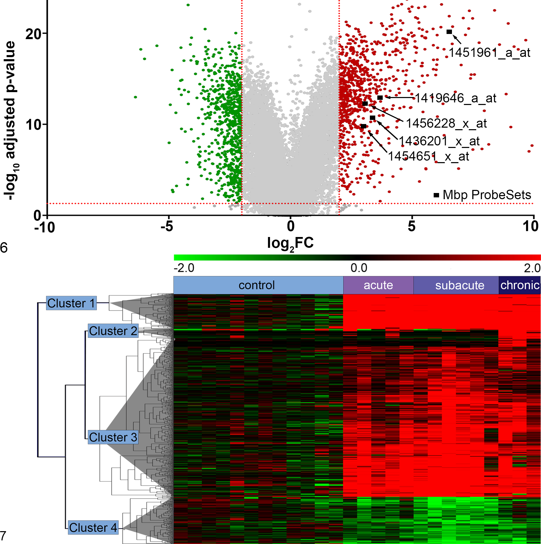
Principle component analysis (Fig. 4) is used for exploratory data evaluation to visualize differences between certain experimental conditions, detect biological outliers, and distinguish specific subgroups in data sets. 2,131 In microarray experiments, each gene and each sample represents 1 dimension in the data set. Thus, it is impossible to visualize the relationship between the expression values of all thousands of genes measured in multiple samples. Several data decomposition/reduction techniques have been introduced for this purpose and here, principle component analysis (PCA) is the most commonly used method. PCA reduces the dimension of the data by constructing a new coordinate system. The principle components of the reduced 2- or 3-dimensional data space are the eigenvectors of a covariance matrix of the data. 2,131 With this reduction, a more convenient view of the data with a focus on the key variables is generated. Thus, the analysis is valuable in obtaining a first visual characterization of the data and helps to discriminate between groups by showing whether and to which degree a separation between groups into subclouds can be found, but also typical response curves or periodic behavior over time among the first principal components may be detected. 128 A vivid example for a possible application of this method from a veterinary pathologist’s point of view is a recent study on canine cutaneous mast cell tumors (ArrayExpress accession number E-GEOD50433; Supplemental Table S1). Using PCA, the authors were able to clearly illustrate expressional differences between mast cell tumors with aggressive and nonaggressive biological behavior. 49
For a review on feature extraction methods, including PCA and available software applications, see Kossenkov et al, 83 Tan et al, 149 and Supplemental Table S3.
Top-Down Analysis of Gene Expression
Following a first visual assessment, the gene expression data are subsequently analyzed using statistical methods. A helpful web page to find freely available programs for the intended analysis is http://omictools.com/.
Selection of Differentially Expressed Genes
The selection of DEGs is a basic technique for comparing expression profiles between different conditions. One main application of microarray analysis is a comparative analysis of gene expression profiles between 2 or more different conditions or phenotypes, the classical class comparison experiment. 89 To understand the biological effects, researchers try to detect which genes are up-regulated (increased in expression) or down-regulated (decreased in expression) in a certain physiological or pathological condition as compared with a reference (control or baseline) condition. 89
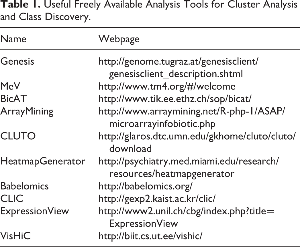
The main problem in the identification of DEGs is to distinguish between true, biologically relevant DEGs and genes that are affected by noise. 36,97 Various different methods to detect DEGs have been introduced and can generally be divided into fold-change methods and statistical testing methods (Fig. 5). Empirical evidence advocates for a combination of a fold-change ranking with a nonstringent, adjusted P value cutoff, as the method of choice to generate highly reproducible lists of DEGs (Fig. 6). 97,138 The fold-change enhances the reproducibility of the data, and the adjusted P value balances sensitivity and specificity and minimizes the impact of different normalization algorithms. 97,138
Fold Change
The simplest method to detect DEGs is to calculate a fold change between 2 conditions. A randomly chosen cutoff value defines a gene as differentially expressed. Cutoff values between 2- and 3-fold are commonly used. 36,143 The main disadvantage of the fold-change method is that because of the randomly chosen threshold, sensitivity and specificity cannot be controlled or quantified. 25,36 Furthermore, the choice of a specific threshold has a high influence on the biological results. 112 Thus, although frequently used in the beginning of microarray technology, the selection of genes based exclusively on fold-change criteria is obsolete. 7,97,36,71,110,125,138
Statistical Testing
When performing statistical tests on microarray data, the user is confronted with the problem that generally thousands of hypotheses are tested simultaneously with a comparably low number of replicates. To extract biological meaningful information from microarray experiments, tailored statistical methods are needed. The statistical algorithms are especially designed to operate large data volumes from high-throughput experiments. In multiple studies, these algorithms were shown to outperform the unstable algorithm of a traditional t test and should therefore be preferred to conventional statistical tests. 36,156
Significance analysis of microarray (SAM) is a popular algorithm introduced by Tusher et al. 156 Two and multiple classes, as well as time series, can be analyzed. 109 However, SAM is reported to perform poorly on noisy data sets. In data with small sample sizes, it is comparable with classical fold-change methods and therefore not recommended for data with these characteristics. 71 SAM is available at http://statweb.stanford.edu/∼tibs/SAM/. A moderate t statistic, called linear model for microarray data (LIMMA), is especially powerful for experiments with a small sample size. 109,141 The LIMMA method is implemented in multiple microarray-analysis applications such as Babelomics (http://babelomics.org/) 4 and Arryanalysis.org (http://arrayanalysis.org/). 38 Other methods preferable when working with a small sample size are BRB t statistic, available as Microsoft Excel add-ins at http://linus.nci.nih.gov/BRB-ArrayTools.html 139,171 ; Cyber-T, provided as a web-based differential analysis tool for 2- and multiple-condition data at http://cybert.ics.uci.edu/ 74 ; and Ranked Product Method (RP), available at http://strep-microarray.sbs.surrey.ac.uk/RankProducts/. 88 In addition, RP has been shown to be robust with noisy and inhomogeneous data. 19,88 Figure 5 shows a comparison of 4 different methods to test for differential expression in a previously published data set 127 nicely illustrating the different levels of sensitivity of the various methods.
Multiple testing procedures
Regardless of the algorithm chosen, a very important topic in microarray analysis is how to deal with the multiple comparisons problem. The statistical algorithms for microarray data perform thousands of comparisons in parallel. 36 Hence, if a conventional t test with a P value threshold of .05 would be applied, parallel testing of 40 000 genes would falsely detect 2000 genes as being differentially regulated. This means that statistical methods have to be adjusted in a way that the false-positive rate (type I error) remains in a tolerable limit. This is done by calculating an adjusted P value. 36,122,146 Classical approaches like Bonferroni or Šidák correction would induce a huge loss of information by increasing the type II error and thus exhibit a rather low power. 36,146 Therefore, more appropriate algorithms such as the false discovery rate (FDR), initially developed by Benjamini and Hochberg, are used. 11,122 Nowadays, multiple modifications have been made to the FDR algorithm and reliably estimate the error rate. 144,146 One widely used modified false discovery algorithm is called pFDR, which estimates a quality called q-value for a particular gene introduced by Storey and Tibshirani. 144 It is suggested that in doubt, the FDR introduced by Benjamini and Hochberg should be used and the adjusted P values should be reported. 122
Venn Diagram
A simple and effective method to visualize DEGs under different conditions or from different time points is by drawing a Venn diagram. 21 Various freely available programs were engineered for this purpose, including applications with area-proportional Venn diagrams (VennMaster; http://sysbio.uni-ulm.de/?Software:VennMaster 79 ), direct transfer of the overlapping groups to related information (BioVenn; http://www.cmbi.ru.nl/cdd/biovenn/ 68 ), or dividing genes by their expression (VennPlex; http://www.irp.nia.nih.gov/bioinformatics/vennplex.html 21 ). The different intersections can subsequently be used for further analysis. 127
Cluster Analysis
Cluster analysis methods facilitate the discovery of new subgroups in clinically or morphologically defined conditions based on their gene expression. Cluster analysis algorithms are used in class discovery experiments, when there is no presumptive knowledge about the data. 17,33 It is based on the idea that genes interact with each other and build groups according to similar expression profiles. 17,33,36 In general, clustering genes is used to identify groups of co-regulated genes or typical spatial and temporal expression patterns during a specific disease course (Fig. 7). Clustering samples is moreover suitable to identify distinct phenotypes, for instance, different molecular subtypes of tumors with morphologically similar appearance. 45 An example for the implementation of this technique in veterinary medicine is presented in Fig. 7 with a microarray study performed on cerebellar specimens of different disease stages in canine distemper. Hierarchical clustering analysis of differentially expressed probes in canine distemper identified 4 clusters with distinct expression profiles. Employing this method, the identification of a distinct cluster of genes only up-regulated in chronic canine distemper (Fig. 7, cluster 2) led to the hypothesis that locally produced autoantibodies and complement may be involved in the exacerbation of demyelination in the chronic stage of the disease. 160
Clustering methods are referred to as unsupervised machine-learning algorithms, which underlines the principle nature of the analysis, that no predetermined knowledge about the data structure is included. 36 Expression profiles are grouped according to their similarity, where the measure of similarity is called the distance. 36 Multiple ways of calculating the distance exist. Euclidean distance is the most commonly applied distance measure. 36 Important to mention is that some clustering algorithms are not necessarily deterministic, meaning that the same clustering algorithm applied to the same data set may produce slightly different results because of their nondeterministic components. 36 The most widely used methods are hierarchical clustering, k-means, and self-organizing maps. 17,124
Hierarchical clustering was the first clustering algorithm used in microarray technology 39 and is still the most popular clustering algorithm. 33,39 Hierarchical clustering is a deterministic method and can be applied to all data, genes, samples, and time points. Hierarchical clustering produces a cluster tree, also known as dendrogram, ending with a single gene or sample (Fig. 7). It is often intuitively displayed graphically as a heat map (Fig. 7). 39 To divide the data in meaningful clusters, the dendrogram has to be cut at a customized level (Fig. 7).
K-mean clustering is a simple and fast method and therefore the most widely used nondeterministic algorithm. 36 The number of clusters has to be chosen in advance by the user. Determining the number of clusters is a great issue. 181 If several classes (eg, experimental conditions) are used, it is suggested to use the known number of classes. 36,181 If the cluster analysis has an exploratory function, it is recommended to repeat the analysis with different clusters and compare the results or to perform an initial PCA analysis to specify the number of clusters. 124,181 The self-organizing map (SOM) is a nondeterministic neuronal network technique. In contrast to the 2 previously mentioned algorithms, SOM provides information about the relationship of the patterns. 124,181 Depending on the distance metric, SOM is robust to noise and outliers. 77
Nonetheless, essential decisions are the choice of not only a specific clustering algorithm but also whether all genes or a subset of genes should be used and whether to use originally scaled data or log-scaled data. 130 Log scale amplifies noise, especially in genes with low expression values; therefore, if low-abundance genes are included in the analysis, it is recommended that the original scale data are used. 130 Genes with an expression value within the background noise should be discarded. 77 Table 1 provides a list of useful freely available clustering tools.
Useful Freely Available Analysis Tools for Cluster Analysis and Class Discovery.
Functional Annotation and Pathway Analysis
Identifying individual genes that show expression changes between different conditions is an important first step; however, from a pathologist’s point of view, most experiments are performed to transfer the results into mechanistic knowledge, which helps to understand the biological or pathological processes involved. Thus, functional annotation of the DEGs or subsets of genes obtained by cluster analysis or other class discovery algorithms is a crucial step when the analyst wants to gain insight into the pathogenesis of a respective disease. In biology, expression changes do not occur independently from each other as the list of DEGs suggests but are part of complex pathways and networks. One way of understanding these interdependencies is to subcategorize the DEGs on the basis of their a priori known functional relationships.
Gene Ontology
In the beginning of microarray technology, the main problem in the functional annotation step was that different formats and vocabularies were used in the existing databases. 6 Therefore, the uniformly structured, continuously updated, expert-curated Gene Ontology (GO) database was developed (http://geneontology.org/). 6 This ontology provides associations between gene products and GO terms in order to annotate genes based on existing biological knowledge. 6 Three independent biological categories are differentiated: molecular function (MF), biological process (BP), and cellular component (CC).
The GO annotation is structured in a treelike system (Fig. 8). Different sources provide freely accessible GO browsers, in which queries for GO terms and genes are operable. Frequently used examples, among others, are AmiGO 2 (http://amigo.geneontology.org/amigo) 6 from the GO-Consortium and QuickGO (https://www.ebi.ac.uk/QuickGO/) 12 from The European Bioinformatics Institute of the European Molecular Biology Laboratory.
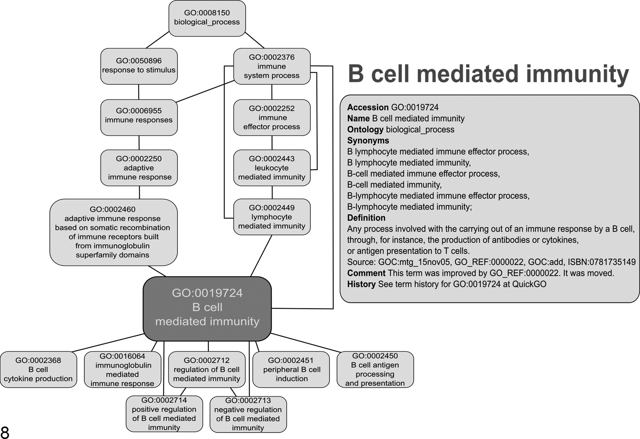
Gene Ontology (GO) term B-cell mediated immunity. The GO structure is exemplified by the GO term GO:0019724 B-cell mediated immunity as represented in AmiGO 2. 26 Shown is the graphical representation of the GO graph containing the input GO term and the term information with accession number, definition, and comments about the term (box).
In addition, the genes associated with GO terms can be used as a gene signature to compare the functional relevance of selected biological processes in the condition of interest based on the frequency of DEGs (Fig. 9). 126 For a review of the GO term database and cross-hybridization techniques for nonmodel organisms as well as potential pitfalls, the reader is referred to Primmer et al. 123
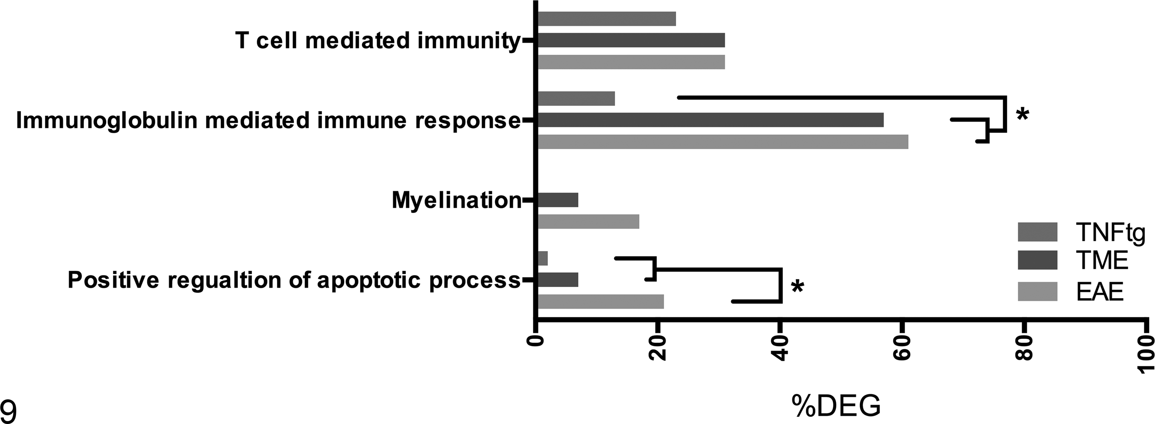
Categorization of data sets using Gene Ontology. The data used here are obtained from a cross-platform, cross-species transcriptomic meta-analysis of multiples sclerosis and its experimental models. 126 The GO terms T-cell mediated immunity, immunoglobulin mediated immune response, myelination, and positive regulation of apoptotic process were selected as gene signatures for specific pathomechanisms using AmiGO. Statistical analysis comparing the percentage of differentially expressed genes within each gene signature across experimental autoimmune encephalomyelitis (EAE), Theiler’s murine encephalomyelitis (TME), and a transgenic tumor necrosis factor–overexpressing mouse model (TNFtg) was performed using Cochrans-Q and post hoc McNemar tests (*P ≤ .05).
Enrichment Analysis
Enrichment analysis is performed to identify the functional associations (eg, specific GO annotations) of a defined list of genes, usually the list of DEGs. 65 The rationale behind enrichment analysis is that if a biological process is abnormal or different between 2 or more conditions, more genes than just by random chance will be associated with this specific process within the list of DEGs. Enrichment analysis is an integral part of almost every transcriptome analysis and provides a valuable general view of processes or functions related to the genes of interest.
A microarray study examining mesenteric lymph nodes in pigs naturally affected by postweaning multisystemic wasting syndrome 41 (ArrayExpress accession number: E-GEOD-19083; Supplemental Table S1), for example, used enrichment analysis to detect overrepresented GO terms in the list of DEGs between infected and nonaffected animals employing Database for Annotation, Visualization and Integrated Discovery (DAVID). A comprehensive list of 95 GO terms was found enriched in the comparison and included terms such as inflammatory response, acute phase response, innate immune response, complement response, cell adhesion, and vesicle trafficking. Subsequent workup led to the conclusive hypothesis that complement receptors as key molecules for the induction of adaptive immunity could be involved in the pathogenesis of postweaning multisystemic wasting syndrome. 41
Different approaches have been developed for gene enrichment analysis purposes.
Overrepresentation analysis algorithms compare the proportion of genes within a preselected list of genes (eg, DEGs), which are associated with a particular functional term (eg, GO term) with the proportion of genes obtained just by random chance. 36,80 Tests implemented in these overrepresentation analyses are chi-square test, Fisher exact test, or a binomial probability and hypergeometric distribution. 36,80 Overrepresentation analysis algorithms are a simple but effective way to gain insight into the biological processes of a simple list of transcripts and to draw conclusions regarding joint functions. However, the tests do not consider expression values associated with the genes and treat all genes equally without considering quantitative differences. 65 Therefore, the quality of the preselected genes highly affects the outcome of the analysis. 65 Furthermore, overrepresentation analysis ignores interdependencies between the different biological processes. 80
Commonly used, freely available and established tools used for such enrichment analyses include DAVID 66 or WebGestalt. 166 However, numerous other tools with similar algorithms have been introduced. 65
Functional Class Scoring Approaches
Functional class scoring approaches overcome some of the limitations of overrepresentation analysis by not requiring preselected gene sets and additionally using the expression values of the genes for the analysis. 80 Thus, they also consider sets of functionally related genes with small but coordinated changes, which would otherwise not pass the preselection thresholds. Most of the applications rank genes in a given functional term according to their expression, which makes the analysis more robust to outliers. Despite these enhancements in comparison to overrepresentation analysis, functional class scoring approaches do not yet take interdependencies of genes and different biological processes into account. 80 A frequently used tool for functional class scoring approaches is Gene Set Enrichment Analysis algorithm, available as a platform-independent execution in the java virtual machine (http://software.broadinstitute.org/gsea/index.jsp), but also implemented in various microarray analysis suites as web tool. 147 Further functional class scoring enrichment tools, among others, are ermineJ 51 or FatiScan implemented in Babelomics. 4,65 For a comprehensive list of pathway tools, please see Khatri et al. 80
Summarized, the results of overrepresentation analysis and functional class scoring algorithms are quite similar, although functional class scoring is thought to create more consistent results than overrepresentation analysis. 65 Overrepresentation analysis is reported to detect commonly known and already anticipated biological processes, whereas functional class scoring algorithms identify substantially more and previously unknown functional relations to biological processes. 126
Pathway Analysis
Pathway analysis aims to detect networks of interdependent or co-regulated genes affected by the different experimental conditions. Biological processes are regulated by a complex system of interactions, and unlike GO, pathway databases try to address this challenge by offering networks of gene or protein interactions or metabolic reactions and signaling pathways. As an example of veterinary interest, O’Donoghue et al 111 (ArrayExpress accession number: E-GEOD-24251; Supplemental Table S1) used this technique in a study on canine osteosarcoma. The authors were not only able to observe differences in dogs responding poorly and dogs responding well to chemotherapy, with respect to pathway modulations for well-known cancer gene signatures such as matrix metalloproteinases, transforming growth factors, wingless-type MMTV integration site family members, and nuclear factor κ–light-chain-enhancer of activated B cells downstream targets, but were also able to demonstrate interaction of affected genes in the hedgehog and parathyroid hormone signaling pathway in bone and cartilage development in their microarray study.
Freely available, commonly used, and most comprehensive pathway databases are KEGG, 73 Reactome pathway knowledgebase, 30 PANTHER pathway, 103 National Cancer Institute-Pathway Interaction Database, 134 and WikiPathways. 118 Most frequently used commercial pathway analysis solutions are Metacore (GeneGO, St Joseph, MO, USA; Fig. 10) and Ingenuity Pathway Analysis (Qiagen, Redwood City, CA, USA). These curated databases are more reliable than protein interaction networks but do not include all known genes or interactions. 107 However, a major problem concerning pathway analysis is that the structure and information content of pathways is nonuniform. 107
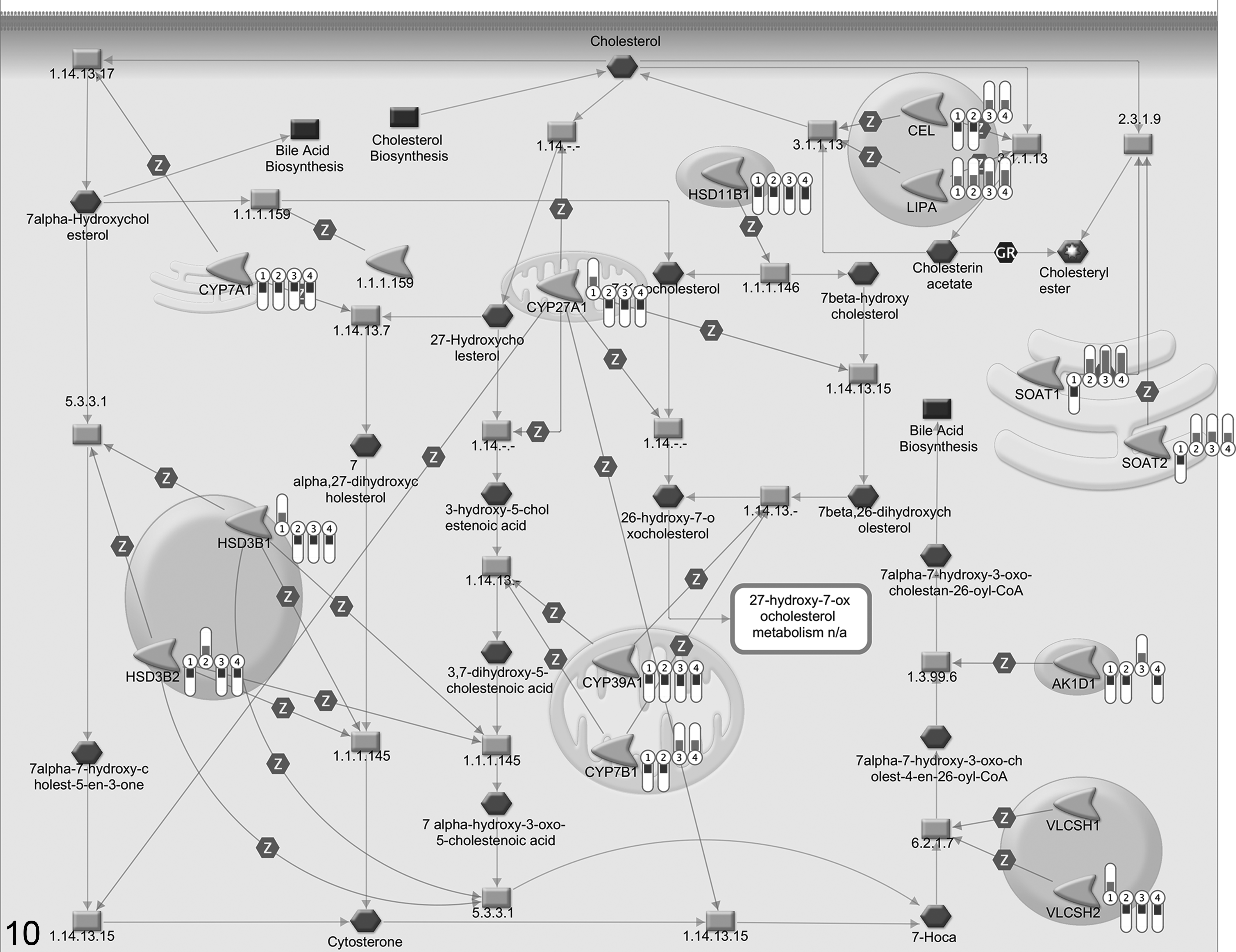
Canonical cholesterol metabolism pathway. Transcriptional changes associated with cholesterol metabolism pathway in a data set from an experiment in Theiler’s murine encephalomyelitis virus (TMEV)–infected mice 159 illustrated in the canonical cholesterol biosynthesis pathway map from Metacore database (GeneGO, St Joseph, MO, USA). The bars labeled from 1 to 4 display the magnitude of the fold changes of significantly differentially regulated genes on 4 different time points. The indicator scale directed downward indicates a down-regulation, and the indicator scale directed upward indicates an up-regulation.
Various tools use pathway databases additionally to GO as a backend database in their enrichment analysis. Examples are Onto-Express, 81 DAVID, 66 WebGestalt, 179 and Fatigo+, 3 among many others. Both overrepresentation analysis and functional class scoring were adjusted for pathway analysis. In these algorithms, the genes in the different pathways or networks are treated as a simple list of genes with the limitations stated above. Pathway topology–based approaches address these problems by using a similar algorithm as functional class scoring approaches but include pathway topology to compute gene-level statistics. 80 The analysis is enhanced by including interaction networks instead of considering pathways as simple collections of genes. 107 For an extensive compilation and explanation of the different algorithms, please see Mitrea et al. 107
Bottom-up Analysis of Gene Expression
Bottom-up analysis is a convenient tool in the hypothesis-driven investigation of a priori defined genes or pathways of interest. It concentrates on predetermined and manually selected single genes or smaller compilations of genes involved in a defined biological process or molecular function. The corresponding gene expression values are conveniently analyzed using conventional statistical tests. Using this approach, the researcher is able to target specific scientific questions based on the involved genes and independently from the global hypothesis-free approach, as presented above.
An example for this approach is represented by a reanalysis of 2 microarray studies on canine mammary tumors (E-GEOD-22516 and E-GEOD-20718) with regard to embryonic stem cell expression. The author hypothesized that common pathways between cancer cells and embryonic stem cells can serve as potential targets for anticancer therapy and as prognostic factors for clinical outcome. 178 The consecutive investigation of literature-based embryonic stem cell gene signatures resulted in the identification of significant differences in the overall survival of dogs with high expression of an MYC-centered gene signature compared with low expression. 178
The hypothesis-driven analysis of the expression data of a priori selected genes systematically differs from the previously described top-down approach of searching the genes and pathways with the highest changes and therefore is named “bottom-up” analysis. Bottom-up analysis of microarray gene expression data starts at the level of normalized gene expression data and generally uses conventional statistical methods and tests. The first step is the selection of interesting candidate genes such as those derived from previous experiments, scientific literature, and pathways. During this step, a frequently encountered pitfall is the numerous synonyms and orthologs of gene names in the different repositories and the literature. Multiple synonyms for the same input gene regularly prevent the second step: the correct assignment of genes of interest to probes. However, multiple software tools such as Ihop (http://www.ihop-net.org/) help to identify the species-specific, official gene name and gene symbol. 42 Once the official gene name is known, the Ensembl genome browser can be configured to display the probes of various commercial microarrays aligned to the genomic DNA and mRNA sequences (http://www.ensembl.org/). 8 Another complementary strategy is the retrieval of associated sequence details from the online resources of the microarray manufacturers followed by manual alignment analysis. However, as stated above, a gene can be represented by multiple probe sets on the microarray. Our example from the mouse Mbp gene shows that there are 8 ProbeSets of the Affymetrix GeneChip Mouse Genome 430 2.0 array targeting the respective genomic region (Supplemental Table S4).
As soon as the probe IDs specific for the gene of interest are known, the associated expression data can be easily retrieved from the preprocessed and normalized gene expression data matrix. Notably, as stated in the introduction, the gene expression data matrixes from thousands of previously performed microarray experiments are commonly stored together with all additional information about the experimental conditions in publically accessible genomic data repositories like ArrayExpress (https://www.ebi.ac.uk/arrayexpress/) or GEO (http://www.ncbi.nlm.nih.gov/geo/). Preprocessed and normalized data are downloadable as .txt files from these repositories and can be processed easily with conventional spreadsheet applications. Further implementations in these repositories such as GEO2 R (http://www.ncbi.nlm.nih.gov/geo/geo2r/) even allow a direct comparison and analysis of differential expression of two or more groups. This enables researchers to extract and analyze the gene expression data concerning their genes of interest from microarray experiments deposited by others.
The next steps after the extraction of the gene expression data are descriptive and inferential data analysis using classical statistical methods similar to the analysis of RT-qPCR or other biological data. 57,58,63,75,86,148 The pitfalls described in the section “Annotation of Microarray Data” for technologies where multiple probes represent a gene are particularly important when using small sets of genes. They highlight the necessity for manual inspection of each probe under investigation and argue against a strategy of automatically calculating the mean of the probes with the same gene identifier.
One major shortcoming of microarray-derived gene expression data is the inherent lack of probe-specific quantitative standardization. This precludes estimation of the absolute amount of mRNA molecules within a specimen as well as determination of the threshold of detection. However, many systems apply spiked-in controls with definitive concentration for assessing the hybridization for different target concentrations. These controls can be used to determine if expression of a target gene is within the range or at the lower or upper border of the assay’s sensitivity, as was applied to the characterization of canine Schwann cells, olfactory ensheathing cells, and Schwann cell–like glia. 158 Many comparisons have revealed a good correlation of microarrays with RT-qPCR, although RT-qPCR clearly has a higher sensitivity, confirming its role as the gold standard for mRNA quantification. 32,58,135,168 Despite the good correlation, a systematic underestimation of high absolute fold changes was observed for microarray data compared with RT-qPCR in multiple studies. 23,32 This compression phenomenon is possibly related to the smaller dynamic range of microarrays as compared with RT-qPCR. 23,32
In conclusion, if publically available microarray data exist from a previously published experiment with a design allowing the actual scientific hypothesis to be addressed, it is worthwhile to manually analyze potential genes of interest in silico. This enables the researcher to obtain reliable results at no cost and no time in the wet lab. As a rule of thumb, when a microarray experiment identifies significant differential expression of a gene of interest, it is considered to be of low priority to confirm the finding by RT-qPCR, whereas confirmatory RT-qPCR may be valuable when the microarray data set identifies no significant difference despite scientifically reasonable suspicion.
Advanced Methods of Microarray Analysis: Biomarker Discovery
Investigations interested in the definition of a molecular pattern, which can be used as an indicator for specific biological processes, and pathological conditions employ biomarker discovery algorithms to find gene signatures, which are able to reliably differentiate between the a priori defined conditions. These class prediction analyses, also referred to as supervised machine learning techniques, are algorithms that, in contrast to the machine-learning techniques used for unsupervised cluster analysis, need additional explanatory metadata (eg, qualitative descriptors such as the assignment to a specific disease or control group or quantitative variables from immunohistochemistry or survival data). The goal of these methods is to extract single or few informative genes, called classifiers, which enable the categorization of further unclassified data. 36 At present, these methods are extensively used in the context of cancer research to extract biomarkers for classification and prognostic evaluation. In veterinary medicine, class prediction tools might be used to discover biomarkers to predict the subtype, stage, prognosis, or appropriate therapeutic options for a disease based on the expression values. 145,152 This technique, for instance, was used to identify transcriptomic biomarkers for the biological behavior of canine mast cell tumors. 50 Employing Prediction Analysis of Microarrays software, available online at http://www-stat.stanford.edu/∼tibs/PAM, the authors were able to detect that malignant transformation was associated with differential expression of 13 genes. According to the authors, multiple genes in this classifier gene list were similarly and repeatedly described in human malignancies as potential biomarkers or therapeutic targets. Subsequent survival analysis showed a significantly increased incidence of mast cell tumor–related mortality for tumors classified as undifferentiated by the algorithm. 50
To implement class prediction techniques in microarray analysis, the data set is classically split into a training and a test set. The training data set with a priori known class affiliation, for example, a specific histologic pattern or clinical outcome, is used to detect general classifiers that are able to differentiate between the groups. These potential biomarkers are subsequently validated on the test set. 36,142 One main issue, as frequently faced when working with microarrays, is the small number of samples per class in comparison with the very large number of features (genes). 142 This generates a problem called “overfitting,” which produces classifiers too specific for a meaningful classification. 5 Thus, a major consideration when using these classification methods is the selection of a relevant subset of genes that are most promising to detect relevant classifiers. Therefore, redundant and noisy features have to be eliminated in the feature selection step. 142 For a robust classification, a sample-to-feature ratio of 5-10 is required, which is rarely achieved in microarray experiments. 142 If the sample size is too small, cross-validation methods can be used. 38,142
The most frequently used classification algorithms for biomarker detection are k-nearest neighbors, 153 classification and regression trees, 16 artificial neuronal networks, 13 and support vector machines. 20,124
RNAseq-Based Gene Expression Analysis
In contrast to hybridization-based microarray methods, RNA sequencing (RNAseq) uses next-generation sequencing (NGS) technologies for transcriptome profiling. Thus, it reveals a complete snapshot of all available transcripts at that precise moment in the cell. NGS allows sequencing of any piece of DNA or cDNA in terms of millions of short reads. It is a powerful tool for quantification of gene expression, detection of splicing variants and single nucleotide variations, and discovery of novel coding and noncoding transcripts or fusion genes. Figure 11 illustrates the difference between the workflow of a microarray experiment and an RNAseq experiment.
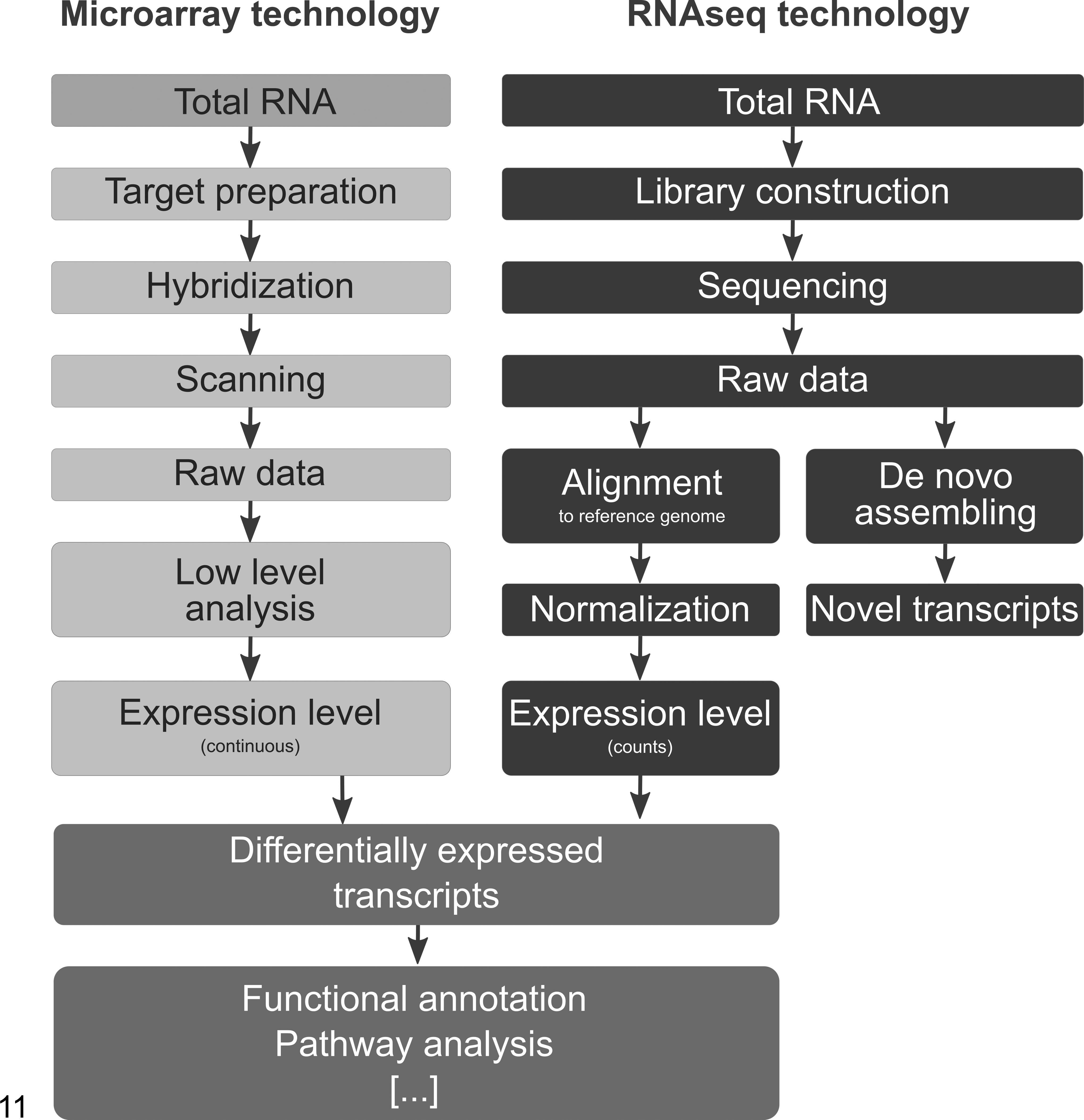
Workflow microarray analysis versus RNA sequencing analysis. The figure illustrates the difference between the workflow of a microarray experiment and an RNAseq experiment.
RNA Sequencing
All currently available sequencing platforms require the generation of a DNA library suitable for high-throughput sequencing. Different protocols have been developed for strand-specific RNAseq library preparation. 96 Each cDNA molecule from the prepared RNAseq library is then sequenced in a high-throughput manner to obtain short sequences from one end (single-end sequencing) or from both ends (pair-end sequencing). Depending on the DNA-sequencing technology used, reads are typically 30 to 400 bp. 170
Various sequencing platforms are available on the market. Each system uses a specific chemistry and sequencing technology and produces reads of variable length with different error rates. A detailed comparison of the different technologies is described elsewhere. 52,91,93,94 All of these platforms generate a variety of file formats that can all be converted to the FASTQ format. The FASTQ format has become a standard interchange file format for NGS data. It combines the sequence and an associated per base quality score. 27
Raw Data Processing
As in microarray analysis, many data analysis methods are available for RNAseq, but no standard protocols are defined. For a review, see Garber et al. 46 Nevertheless, protocols for typical steps have been proposed and are widely used. Several publications from the Food and Drug Administration Sequencing Quality Control project demonstrated a comprehensive assessment of RNAseq accuracy, reproducibility, and information content. 136 Results from this consortium might help to develop a standard for the analysis pipeline.
Frequently, the raw imaging data for each RNAseq cluster are converted directly into a FASTQ file containing sequences and quality scores for each base of one read. The following data analysis workflow comprises 3 main steps: the alignment of these reads to an annotated genome, assembling into transcripts, and quantification of gene expression (Fig. 12).
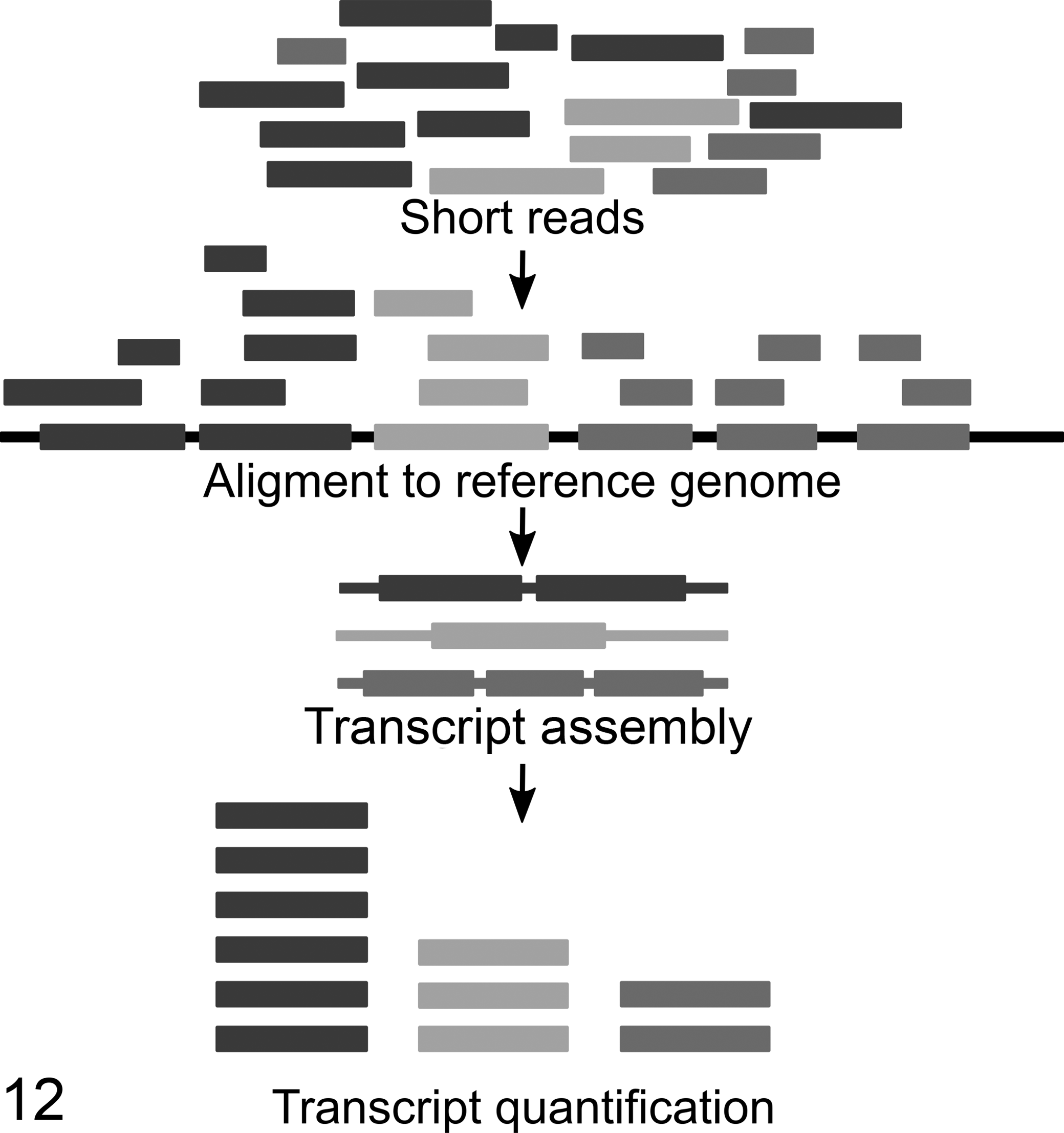
Workflow of RNA sequencing raw data analysis processing. After sequencing, the obtained short reads are aligned to a reference genome and assembled into transcripts. After that, the expression level is quantified by counting the number of reads mapped to a specific region.
For RNAseq and the required transcriptome alignment, a number of splicing-aware mapping tools have been developed. 87 These include Genomic Short-read Nucleotide Alignment Program (GSNAP), 172 MapSplice (http://www.netlab.uky.edu/p/bioinfo/MapSplice), 167 RNA Seq Unified Mapper (RUM; http://cbil.upenn.edu/RUM/), 54 Spliced Transcripts Alignment to a Reference (STAR; https://code.google.com/p/rna-star/), 35 and TopHat (https://ccb.jhu.edu/software/tophat/index.shtml). 154 Each of them has specificities (eg, with respect to speed and performance).
Transcript quantification read sequences are then counted and assembled into full-length transcripts (Fig. 12). For gene expression estimation, read counts must be normalized to correct for systematic variability, such as library fragment size and read depth. Therefore, a widely used algorithm is used: the reads per kilobase of transcripts per million mapped reads (RPKM). It normalizes the read count by both the gene length and the total number of mapped reads. For paired-end reads, the “paired fragments per kilobase of transcript per million mapped reads (FPKM) metric” is used. 87,155 Several publications claim that for the measurement of RNA abundance with RNAseq, a slight modification of the FPKM/RPKM metric would be required as it does not correctly measure the relative molar RNA concentration. 90,163 The metric proposed by Wagner et al 163 is called transcripts per million (TPM). TPM respects the property that there is an average invariance of the number of mapped reads between different sets of transcripts. RPKM or FPKM do not respect this invariance.
Some of the available software tools for transcript assembling and quantification rely on the assembling by comparison to a reference genome, some others also provide a de novo read assembling (eg, Cufflinks, FluxCapacitor, iReckon). Examples for algorithms available for analysis of differential gene expression are Cuffdiff2, DESeq, edger, and BaySeq. 87
Currently, a huge number of open source interfaces were developed to make RNAseq analysis steps accessible to life scientists without deep bioinformatics skills. An overview of these interfaces as well as an evaluation of 6 of the more widely used tools is provided by Poplawski et al. 121
The sequencing depth (number of sequenced reads) between studies varies depending on the scientific question behind the RNAseq experiment. For the detection of rare splice events or new, lowly expressed transcripts (eg, noncoding RNAs), a very deep sequencing (>80 million reads per sample) is required. However, for the expression analysis of abundant transcripts (more than 10 FPKM) across different conditions (eg, time points, chemical treatment), a sequencing depth of 36 million reads per sample may be sufficient. 140
Differences Between Microarray and RNAseq Data
RNAseq data are fundamentally different from microarray data. In the case of microarrays, the scanner returns signal intensities for each probe on the array after hybridization (Fig. 11). In contrast, RNAseq provides the quantification signal in terms of number of reads mapped to a specific region. 100 Recently, it has been shown that RNAseq is more accurate over a larger dynamic range of gene expression than expression microarrays. 101,163 Furthermore, it is clearly superior to microarrays for its ability for de novo discovery of previously unknown sequences and detection of genes with low expression. 53,84,165 An advantage of RNAseq is also its ability to quantify the whole transcriptome, which is not possible with microarray analysis. 72
However, the workflow for biological interpretation of mRNA expression data from RNAseq is very similar to that used for microarray data analysis. Instead of probe identifiers, Ensemble Gene ID or RefSeq are used for the analysis employing the above-described applications (Fig. 11). Therefore, many methods presented in this review can easily be applied in the same way to data obtained by RNAseq.
Conclusion
High-throughput transcriptome analysis methods have conquered various fields of application, including screening for diagnostic and prognostic expression profiles or identifying key genes and pathways correlated with biological processes or diseases. As the tremendous amount of freely accessible data in public repositories shows, the challenge of future research will no longer be the generation of data but rather the analysis and interpretation. Notably, veterinary pathologists do not have to be computer scientists or statisticians to take full advantage of these technologies. Numerous user-friendly applications are available for researchers without programming skills. The increasing utilization of these technologies in veterinary medicine will gradually revolutionize veterinary research and diagnostics and will shift the focus to a global systems biology approach, in which the pathogenetic expertise of veterinary pathologists is highly needed to translate high-throughput transcriptome data into reasonable biological knowledge.
Footnotes
Declaration of Conflicting Interests
The author(s) declared no potential conflicts of interest with respect to the research, authorship, and/or publication of this article.
Funding
The author(s) disclosed receipt of the following financial support for the research, authorship, and/or publication of this article: The research underlying this review was in part supported by Niedersachsen-Research Network on Neuroinfectiology (N-RENNT) of the Ministry of Science and Culture of Lower Saxony, Germany, and by the European Union’s Horizon 2020 research and innovation program under grant No. 643476 (COMPARE).
References
Supplementary Material
Please find the following supplemental material available below.
For Open Access articles published under a Creative Commons License, all supplemental material carries the same license as the article it is associated with.
For non-Open Access articles published, all supplemental material carries a non-exclusive license, and permission requests for re-use of supplemental material or any part of supplemental material shall be sent directly to the copyright owner as specified in the copyright notice associated with the article.