
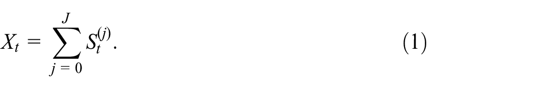
Abstract
Understanding time series signal extraction is vital for federal agencies, especially as data collection accelerates. One natural extension is moving from univariate to multivariate signal extraction, which offers the promise of reducing extraction error by exploiting cross-sectional relationships. However, such an extension ushers in new computational challenges, viz. larger parameter spaces and more complicated objective functions. The Expectation-Maximization (EM) algorithm provides a methodology to implicitly compute (or approximate) maximum likelihood estimates (MLEs). This paper provides methodology for applying the EM algorithm to a class of latent component multivariate time series models that allow for a nuanced specification of the unobserved signal. We derive an explicit formula for the maximization step, which facilitates computation speed while also improving the stability of the algorithm. Numerical studies demonstrate EM’s ability to efficiently compute MLEs in low-dimensional systems, while also providing feasible estimates in moderate-dimensional systems where MLEs are infeasible to compute. Applications to monthly housing starts and daily immigration are provided.
1. Introduction
Multivariate signal extraction can be accomplished through the use of latent component models (McElroy and Trimbur 2015), for which the number of parameters typically increases as a quadratic function of dimension. Heuristically, this is because the linear filtering theory is built upon a knowledge of variance and covariances, that is, for
From the perspective of signal extraction, obtaining parameter Maximum Likelihood Estimates (MLEs) is only a means to the end of constructing a model-based linear filter. Hence, premature terminations of the nonlinear optimization (resulting in saddle-points or local optima) may be adequate for the practitioner objectives. In the case of the Gaussian likelihood, the objective function is optimized by minimizing one-step ahead forecast error, and therefore the filters constructed from such premature terminations may still perform well. Nevertheless, there are some features of the model fitting that are absolutely vital to the performance of signal extraction filtering: (i) the signal-to-noise ratios (snr), which are determined by estimates of variability for different components; (ii) cross-correlations between series, with respect to a particular signal dynamic.
The failure to obtain accurate snr estimates results in either under- or over-smoothing. Under-smoothing refers to an incomplete extraction of the signal that is actually present, and by necessity some of this signal will be leached into other components—this is a critical failure in an application such as seasonal adjustment. Over-smoothing refers to poaching signal content that is spurious, or not really present, essentially from stationary oscillations in other components, thereby destroying structure that may be of interest. For example, seasonal adjustment filters that have a spectral trough that is too wide can potentially alter and disrupt the business cycle component (McElroy 2012). Over- and under-smoothing can also arise in trend extraction, whereby the use of a moving average trend filter that is either too long or too short yields, respectively, an over-smoothed or under-smoothed trend.
A danger of over-stating cross-correlation patterns is that collinear models may be fallaciously adopted (McElroy and Jach 2019), resulting in so-called common components (e.g., common trends, common seasonals, etc.) in the model Zuur et al. (2003). This results in filters that strongly rely upon cross-sectional filtering rather than temporal weighting. When such collinearity patterns are not truly present in the data, dynamics from one series are spuriously imposed upon another. Under-stating the correlations is a less serious offense—if there is no cross-correlation, the problem reduces to univariate filtering, and we suffer efficiency losses, that is, less precise extraction of the signal.
Whereas straight likelihood maximization may avoid the pitfalls of snr and cross-correlation, the computational challenges mentioned above have motivated other approaches, such as the method of moment (MOM) estimators of McElroy (2017). Although these MOM estimators are consistent (McElroy and Roy 2023) and computationally feasible, being given by an analytical formula only involving linear combinations of sample autocovariances, they do suffer from deficiencies. In particular, these estimators can yield covariance matrix estimates that have negative eigenvalues; the closest positive definite approximation, obtained by setting any negative eigenvalues to zero and reconstructing the matrix with the same eigenvectors, yields a singular covariance matrix wherein spurious collinearity has been infused.
Another approach, based on work of Shumway and Stoffer, is to use the Expectation-Maximization (EM) algorithm (Dempster et al. 1977) to implicitly compute MLEs, or perhaps approximate the true MLEs (Shumway and Stoffer 1982). EM proceeds first by the concept of a complete data likelihood, which in this context amounts to considering the data jointly with the signals of interest (see Chapter 8 of Little and Rubin (2019)). Using log Gaussian likelihoods, the conditional expectation operator is applied (the E-step). At this point, we suppose this expectation operator is based upon prior knowledge of the parameters, that is, the values of the parameters obtained from an earlier iteration of the iterative algorithm. However, there are other quantities in the likelihood that depend upon the true, unknown parameters, and at this stage (the M-step) we optimize with respect to these, in the hope that a simple formula will emerge, or at worst that the numerical optimization will be easier than direct likelihood maximization. With these new updated parameters, one computes signal extraction estimates, along with their error covariances, as these are required in the next E-step.
In this article we study a special case of the component models driven by vector white noise considered by McElroy (2017), wherein all the white noise covariance matrices have full rank. We show the M-step yields an explicit formula for the white noise covariance matrices, and this formula can be computed from a knowledge of the extracted signal and the error covariances. This formula is fast to compute (no matrix inversions), and hence the speed of the method depends on our computational facility with signal extraction. In high-dimensional problems, the extraction of a signal takes an amount of time—using State Space (SS) methods, or the recursive approach of Ecce Signum (ES; an R package developed by the US Census Bureau to compute multivariate signal extraction and forecasting results for data with ragged edge missing values; see McElroy and Livsey (2022) and www.github.com/tuckermcelroy/sigex)—roughly comparable to, or a little longer than, a single likelihood evaluation. Whereas our main results (Theorems 2 and 2) can be applied under either an SS or ES paradigm, we have developed our numerical results under the latter computational framework because ES provides the requisite error covariances at all lags using efficient recursive methods described in McElroy (2022). These error covariances are not a standard output of a Kalman filter/smoother algorithm (although the error variances are indeed calculated), and typically require a custom implementation of the SS iterations; for example, Shumway and Stoffer (1982) developed a custom SS routine to generate the lag one error covariances, which was sufficient for their application. In our more general context, such error covariances are potentially needed at all lags. However, the choice of ES by the authors for implementation does not preclude the application of this paper’s EM methods within an SS framework.
When estimating high dimensional multivariate models it is commonplace to employ Newton-Raphson (NR) type optimization routines. These routines are not guaranteed to improve the likelihood for each iteration; decreases to the likelihood in the short-term can be helpful for skipping over local optima. In contrast, successive iterations of the EM algorithm always improve the likelihood and converge to a stationary point (Shumway and Stoffer 1982; Wu 1983). Additionally, there has been considerable development to improve the stability and speed of EM (Jamshidian and Jennrich 1997; Liu et al. 1998). For high-dimensional parameter spaces, the EM method has a speed advantage over NR methods because fewer likelihood evaluations are required, and moreover there is no need to compute numerical derivatives. Furthermore, EM parameter estimates by construction inherit the relevant properties (e.g., estimates of covariance matrices given in Equation (11) below are symmetric and non-negative definite), whereas numerical optimization routines (such as NR) typically require a re-parameterization to enforce these properties. However, the rate of convergence of EM methods near an optimum can be slow; neither NR or EM can avoid the possibility of finding local optima, though the risks can be mitigated by utilizing informative initial conditions—such as MOM or univariate ML (assuming no cross-correlations) parameter estimates.
The rest of the article proceeds as follows: in Section 2 we outline the modeling paradigm and define structural models. The only parameters of these simple models are the covariance matrices of latent processes’ innovations, and our main result in Section 2 provides the M-step for such covariance parameters in a closed form. Then in Section 3 we discuss the algorithmic details, including pseudo-code and convergence criteria specifics. Sections 4 and 5 give numerical studies, as well as applications to monthly housing starts and daily immigration. We conclude with final remarks in Section 6.
2. Methodology
Consider an
A leading example is furnished by
In general, we formulate the signal extraction in terms of difference-stationary processes. Hence we adopt the following assumptions: there exist relatively prime scalar differencing polynomials
It follows that
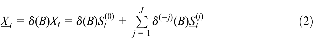
is covariance stationary with mean zero. It is convenient to introduce the notation

These denote stationary components that have been over-differenced.
Our goal is to develop an expression for the Gaussian likelihood in terms of these latent processes, as we endeavor to develop a so-called complete data likelihood. To proceed, we must make some assumptions about these latent processes. We suppose that all the differenced latent processes
where
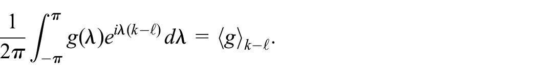
(This defines the notation
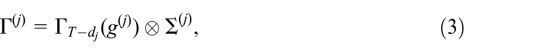
The block Toeplitz covariance matrices for the over-differenced vectors have an expression that is similar to (3): letting

for

where
This assumption generalizes Assumption

(We use lower case for realizations of random vectors.) So up to constants, this is the log of the likelihood of the differenced data, or
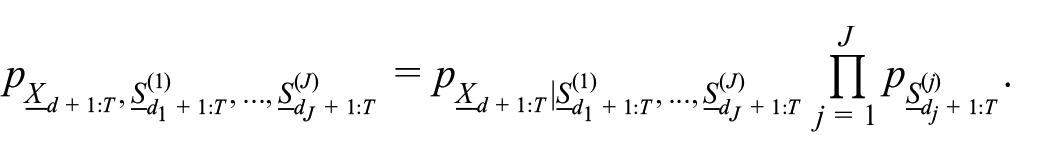
The first pdf, that is, the data conditional on the signals, on the right hand side of the equation is equal to the pdf of the over-differenced irregular evaluated at
noting that
where
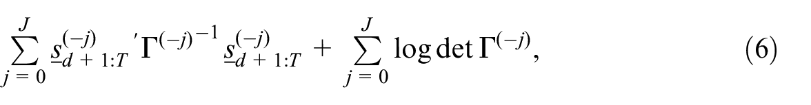
Proof. To the expression in Equation (6) is applied the conditional expectation with respect to the data (for this purpose, we consider random vectors rather than realizations in the above). Under Assumption

which we denote by

applying the conditional expectation operator yields

Next, we apply Equation (8) in the case of each over-differenced signal
Theorem 1 produces the E-step of the EM algorithm, wherein all the signal extraction estimates
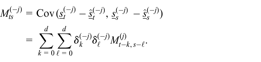
The matrices
for
The M-step estimators of
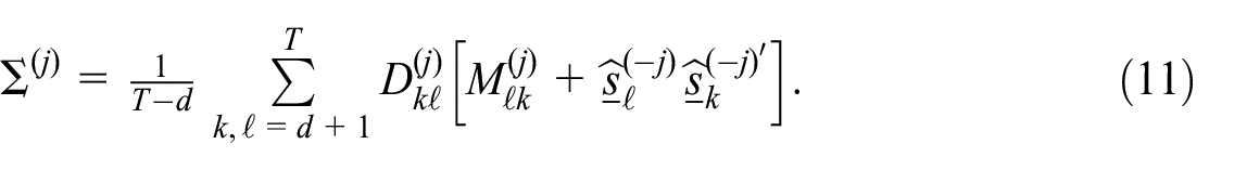
These estimators are symmetric, non-negative definite, and unbiased.
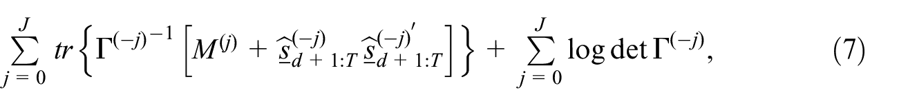
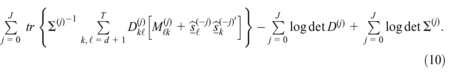
Proof. The expression for the conditional expectation of the complete data divergence Equation (10) follows at once from Equation (7) and Equation (9). In seeking to optimize the expected complete data divergence with respect to one of the matrices
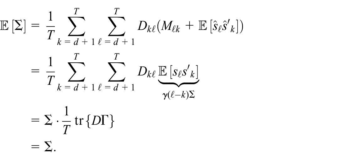
This shows the estimator is unbiased. Next, let
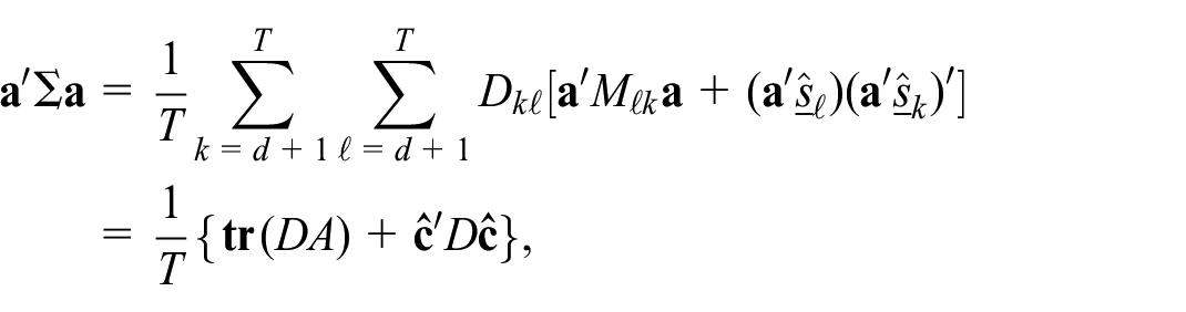
where

is also non-negative definite. Thus
For example, for a lag
With the methodology developed by Theorems 1 and 2, we can construct an EM algorithm for signal extraction—this is discussed in Section 3 below.
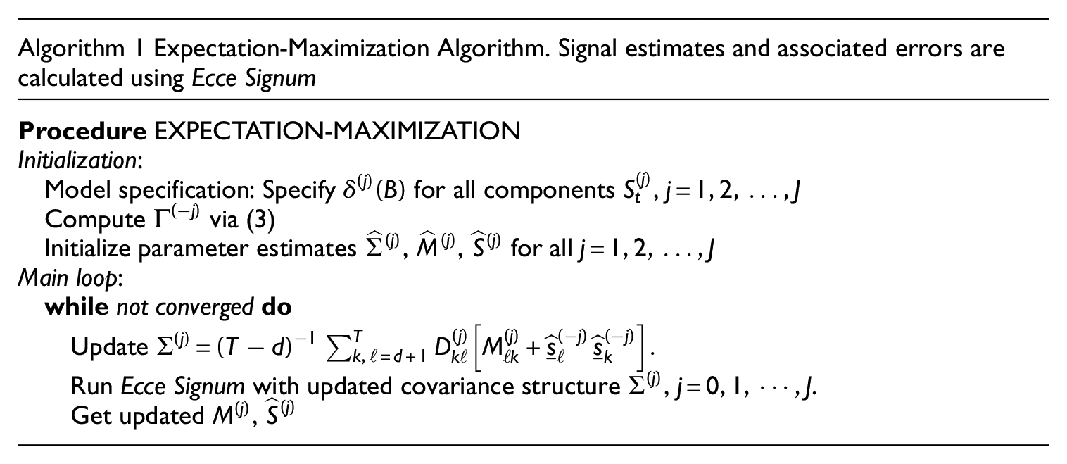
3. Computation
We now discuss the implementation of the EM algorithm, which involves calculation of signal extraction estimates (the E-step) followed by updating the covariance matrix estimates (the M-step) using the formulas in Equation (11). Theorem 2 guarantees that each
If adopting an SS approach to the calculation of these quantities, one could utilize a diffuse smoother with the original data for signal extraction; see Kailath et al. (2000) and Gómez (2016) for details. A so-called “square root” version of likelihood and smoother recursions is available, and has been successful in avoiding numerical difficulties in other settings (Marczak and Gómez 2017). Alternatively, with the ES approach (which we have adopted in our implementation) a faster, approximate approach to the calculation of
A fully specified model will have
Termination of the algorithm occurs at convergence. Numerically, this amounts to deciding on an objective distance between successive parameter estimates. Since we are studying covariance matrices, the choice of matrix norm and termination distance can have an impact on the run time of the procedure. In this article we utilize the absolute distance between successive divergence values as our criterion. At the
The Gaussian divergence
4. Numerical Studies
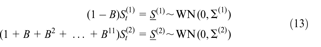
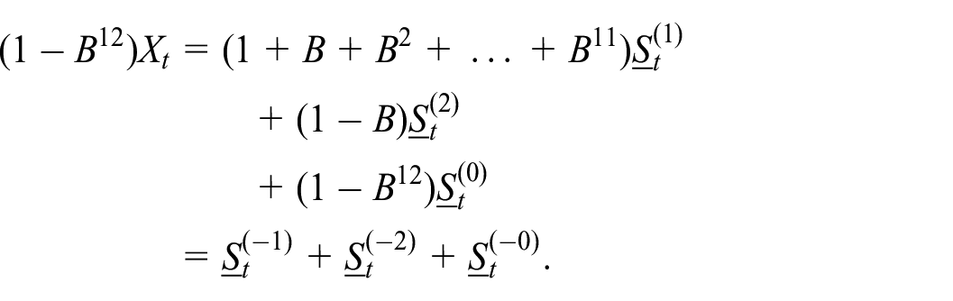
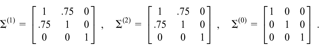
We consider a series with two non-stationary components

where
Here,
We assume the dimension of each component is
A simulated path from this model is displayed in Figure 1. Notice the similar movement in the trend and seasonal pattern for Series 1 and Series 2.
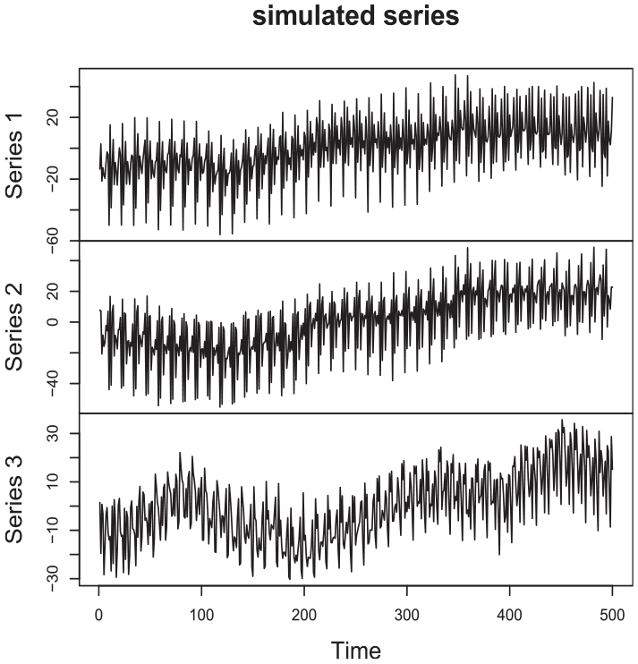
A sample path from a three-dimensional process. The trend and seasonal components of the first two series are positively correlated. The third series is independent of the first two.
The EM algorithm proposed in Section 2 was applied to two hundred realizations of this process. The modest dimension of the process facilitates direct numerical optimization of the likelihood, allowing us to make direct comparisons to the ML results. (Note that for a higher-dimensional processes such comparisons are less feasible, due to computational challenges in obtaining the MLEs.) The Gaussian likelihood of the model given by Equation (12) and Equation (13) is described in McElroy (2017), and is calculated as described in Section 3; hence we are also able to calculate the Gaussian divergence at both the true parameters and the MOM estimators. The value of the Gaussian divergence at the true parameters is used as a basis for comparison, and its value at the MOM estimators is used to understand how far the Gaussian divergence has been reduced by both the ML and EM procedures (since both the ML and EM routines are initialized at the MOM estimates). The results show that both the ML and EM procedures yield significant improvements over the simple MOM estimator. Not only are the EM estimates close to the MLEs in most of the cases, but both also yield values of the likelihood that are in the vicinity of the likelihood evaluated at the true parameters.
Box plots of these four Gaussian divergence values for all replicates are shown in Figure 2. As for the parameter estimates themselves, the results are quite promising. Boxplots of all twenty-seven scalar entries of the three covariance matrices
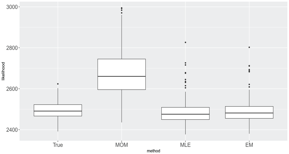
Boxplot of Gaussian divergence values for all two hundred replications of
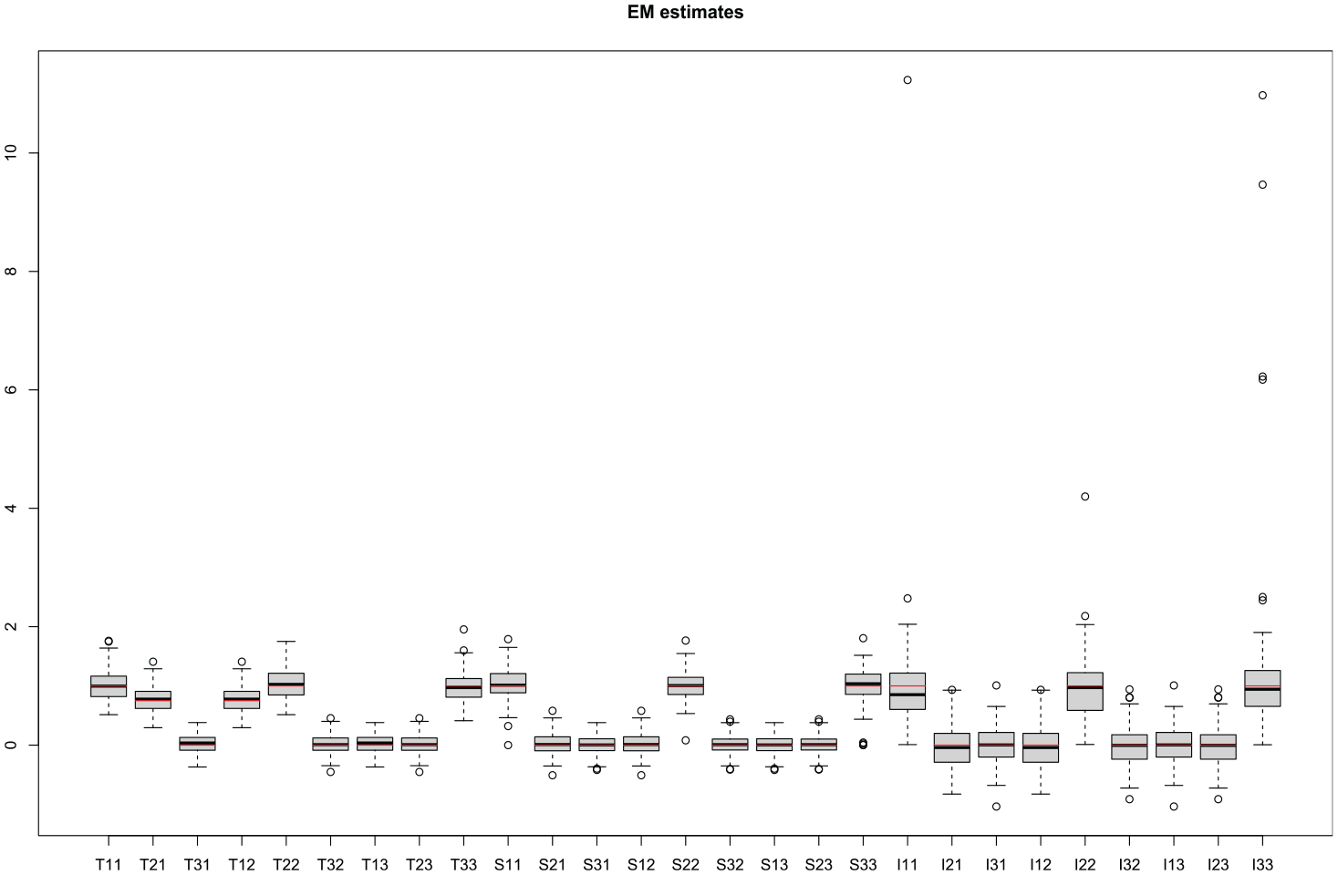
Boxplot of EM estimates for all two hundred replicates and all twenty-seven scalar entries of
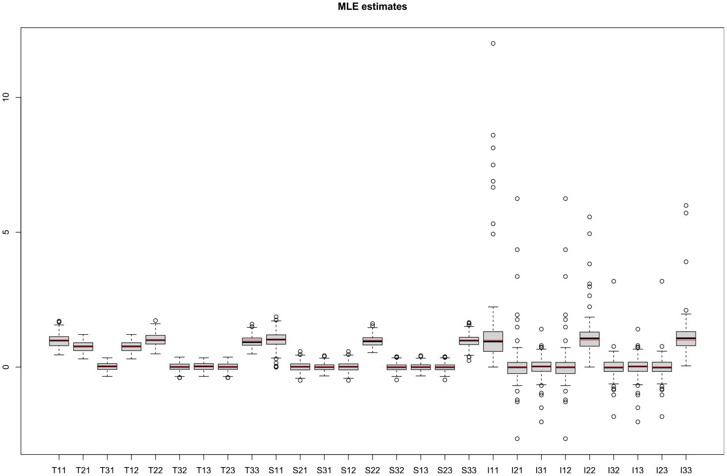
Boxplot of MLEs for all two hundred replicates and all twenty-seven scalar entries of
We also investigated the timing results for ML and EM estimation. Specifically, we simulated data from different sample sizes
5. Application
We investigate two data examples of our methodology. We first consider a four-dimensional monthly housing starts example from the Survey of Construction at the U.S. Census Bureau. Second, we examine a six-dimensional daily immigration series provided by Statistics New Zealand. The housing starts data is of small enough dimension and length that it can be fit via ML, so that we can make a comparison to the parameter estimates of our proposed EM procedure. In contrast, the daily immigration data is only feasibly fitted by EM, being too large to permit calculation of the MLEs. (In McElroy and Livsey (2022) this same immigration series was fit with ML to a reduced data span; this took weeks and multiple restarts of BFGS from new initializations to converge.)
5.1. Housing Starts
The U.S. Census Bureau’s Survey of Construction provides current national and regional statistics on housing starts, completions, and characteristics of single-family housing units and on sale new single-family houses. The four series are from the Survey of Construction of the U.S. Census Bureau, available at https://www.census.gov/construction/nrc/historical_data/index.html. Data was retrieved from this site in June 2021. Information on the the Survey of Construction can been found at https://www.census.gov/construction/soc. Data collected includes start date, completion date, sales date, sales price (single-family houses only), and physical characteristics of each housing unit, such as square footage and number of bedrooms. Each month, housing starts, completions, and sales estimates derived from this survey are adjusted by the total numbers of authorized housing units (obtained from the Building Permits Survey) to develop national and regional estimates. Estimates are adjusted to reflect variations by region and type of construction, and to account for late reports and houses started or sold before a permit has been issued.
Here we focus on single-family housing starts for each of the major four regions in the United States: South, West, Northeast (NE), and Midwest (MW). The housing starts time series for these four regions is plotted in Figure 5. Visually, there is clear monthly seasonality as well as similar trends. Seasonal adjustment for production release of this data is accomplished with a standard univariate
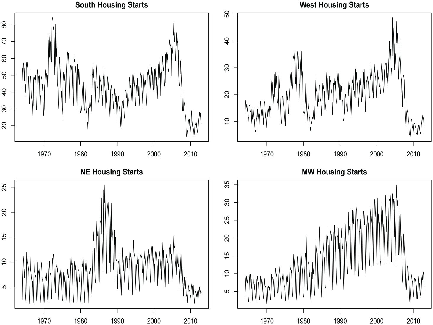
Single family home housing starts broken up by region within the United States. The four regions are the Northeast (NE), South, Midwest (MW), and West. Data comes from the US Census Bureau’s Survey of Construction.
In the multivariate setting we proceed with the same model setup as in Equation (12). Preliminary analysis of the data leads to a trend component requiring a second difference and seasonal sum for the seasonal component. Hence we end up with
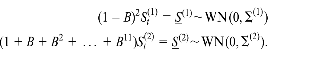
This implies that our full differencing operator is
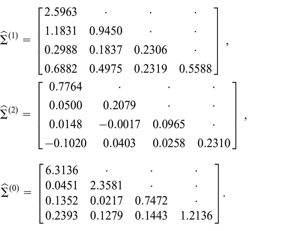
For this model we initialized parameters at default values of
Results from the EM model fit for the South and West are shown in Figure 6. The NE and MW regions have similar plots. It should be noted that the MLEs were obtainable for this series; the dimension of the housing starts data is
Residual diagnostics and properties of the signal extractions are not further investigated here, as the focus of this manuscript is on presenting and implementing Algorithm 1. The code and methodology used in ES provide signal extraction uncertainty; Figure 6 displays the data, trend, and seasonal components.
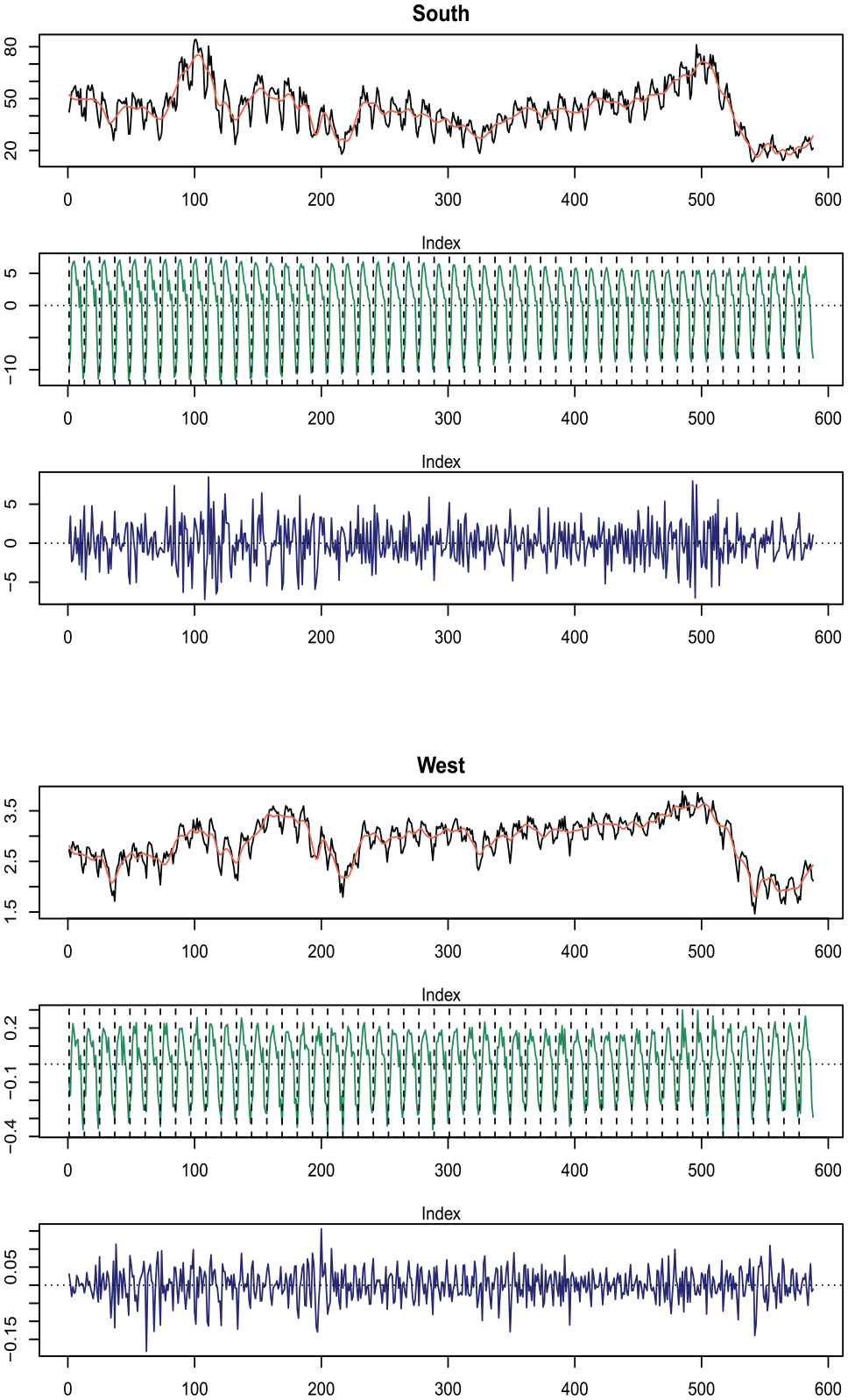
Signal extraction estimates for parameters obtained using EM algorithm. The top three plots are for the South region and the bottom three are for the West region. The original series is in black, trend estimates in red, seasonal component in green, and the irregular in blue.
5.2. Daily Immigration Data
Here we investigate NZ immigration data. The series consists of New Zealand residents arriving in New Zealand after an absence of less than twelve months. These are public use data produced by Stats New Zealand via a customized extract, and correspond to a portion of the “daily border crossings—arrivals” tab (Total) of the Travel category in the Covid-19 portal: https://www.stats.govt.nz/experimental/covid-19-data-portal. The data was downloaded in June 2021. The six-variate series is broken down by the type of person entering or leaving the country. Specifically, the six variables are:
The data is plotted in Figure 7 along with a trend line superimposed. The full dataset consists of 5,114 total observations, beginning on September 1, 1997; additionally, a three-year subspan is plotted in Figure 8 to highlight the within-year seasonal patterns present. A more nuanced model is needed for this daily series beyond those presented for the housing starts data in Subsection 5.1. This is primarily due to the larger number of seasonal patterns present in daily time series, as compared with monthly series. Naturally, the aggregation from daily to monthly will mask many seasonal patterns. For example, the Christmas holiday always occurs in December for a monthly series, so its signal can be directly attributed the the seasonal component in a model of the type in Equation (12). However, Christmas does not always occur on the same day of the week and hence the exact dynamics associated with the holiday season immigration change from year to year (Cleveland and Scott 2007; McElroy et al. 2018; Ollech 2021).
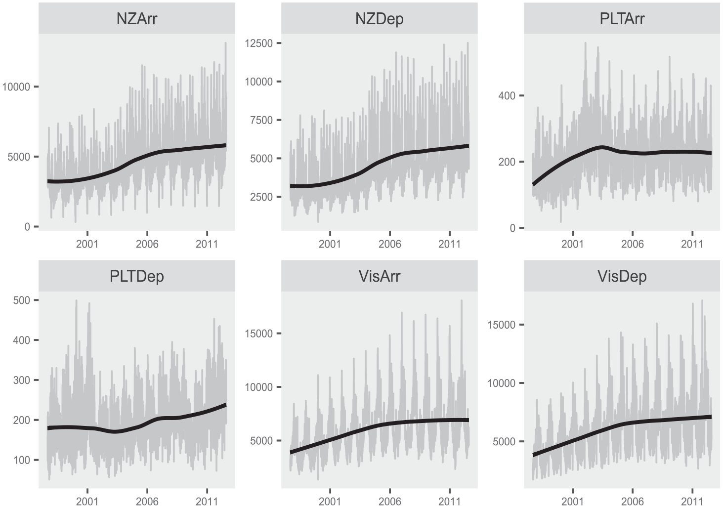
Daily immigration data shown in gray for full span available. The black line is a local polynomial regression fit superimposed to show the long-term trend.
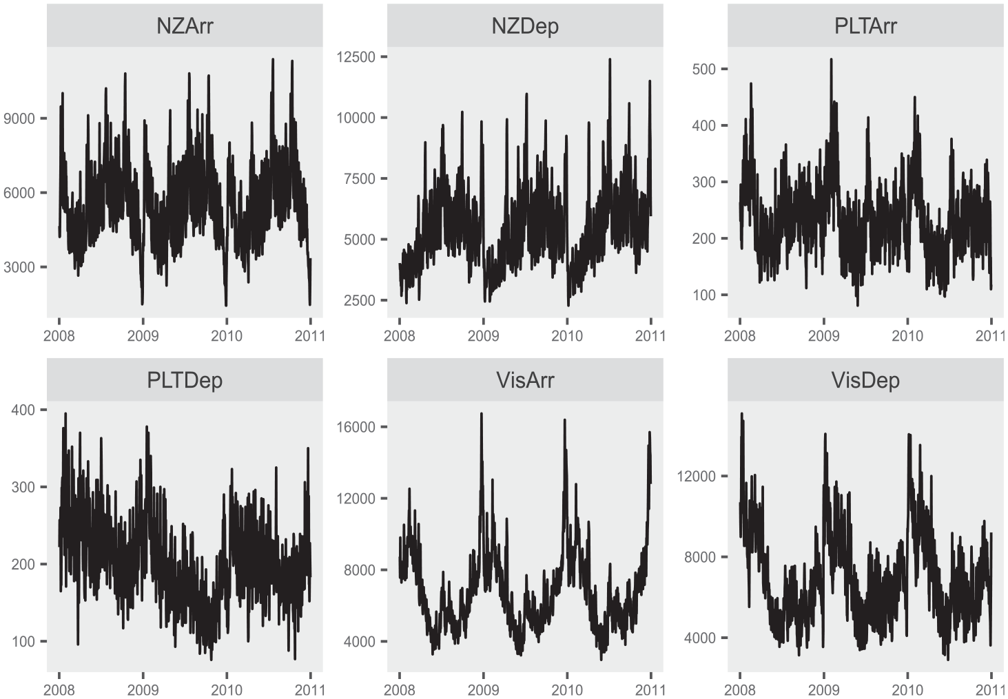
Daily immigration data for 2008 through 2011. The full dataset spans from September 1997 until mid 2011, but the limited window is utilized to better display the daily seasonality.
The spectral densities of the six immigration series are plotted in Figure 9. Peaks in the spectrum give a natural starting point for the identification of models for the components. Vertical lines are shown to indicate frequencies that have historically been shown to impact economic time series. The red vertical lines are at all multiples of weekly frequency. This can be seen as a sinusoidal cycle every 365/7 time points. These peaks correspond to activity due to the day of the week. The green vertical line is the monthly frequency of twelve occurrences per year, and the annual frequency of 1 is given as a blue vertical line. It should be noted here that it is a difficult signal extraction problem to distinguish the trend and the annual component. This is due to the proximity of frequency 1/365 (the annual frequency) to frequency zero (corresponding to the trend).
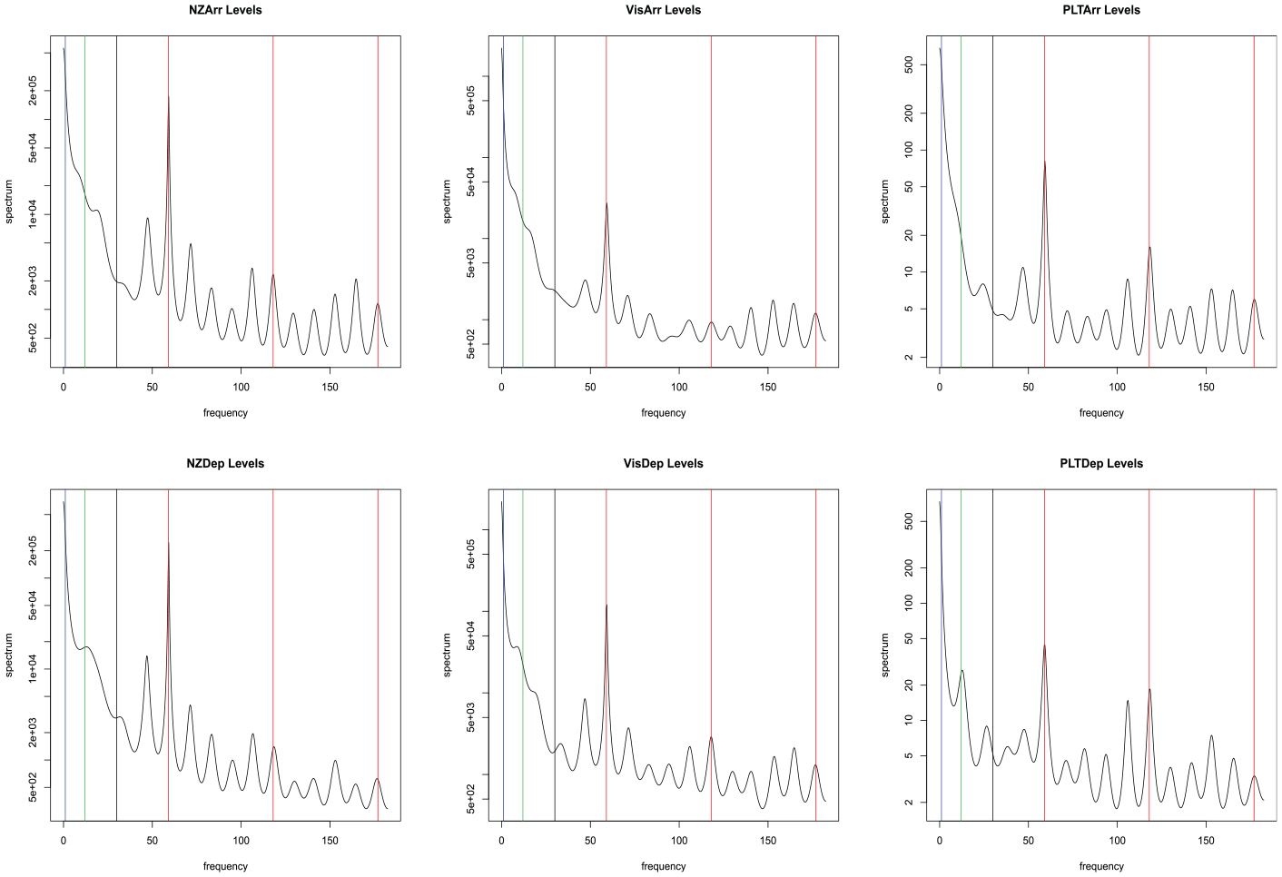
Spectrum for daily immigration data. Vertical lines indicate weekly (red), monthly (green), annual (blue), and trading day (black) effects.
These time series were analyzed in McElroy and Jach (2019), which argued that seasonal differencing, that is, application of the differencing polynomial

where

Each component on the right hand side of Equation (15) is an atomic weekly signal corresponding to one of the three weekly frequencies (

where
Algorithm 1 was run with the specification Equation (14), using the convergence criteria discussed in Section 4 (and used in Subsection 5.1). The moderate dimension and large sample size together result in a long run-times. The ML method has proven to be, at present, infeasible for a model of this complexity, so only MOM and EM are viable. The estimated signals from the fitted model are shown in Figure 10. The y-axis of these figures has been omitted since the extracted components have been offset for visual appearance. We can see the VisDep series has the smallest variance in the irregular component, while the PLTDep has the largest variance in the irregular component. The weekly component broken up into the three atomic weekly components is plotted in Figure 11. Again, the y-axis is omitted since all components are offset to avoid over-plotting.
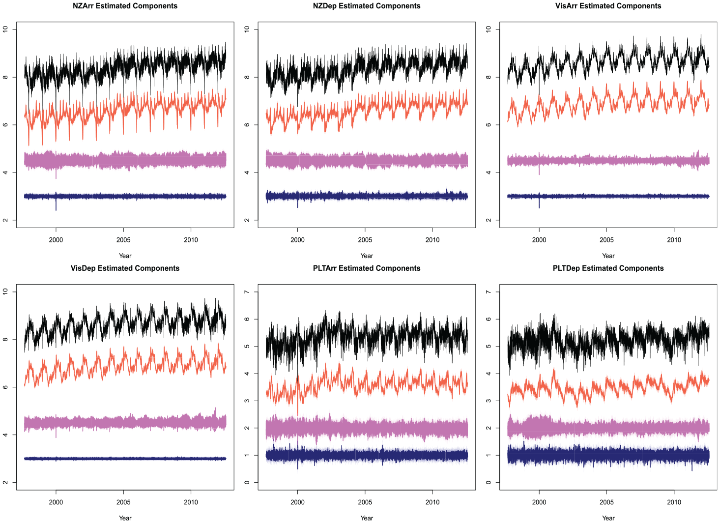
Estimated components for daily immigration data. The original data is in black, estimated trend component in red, weekly seasonal estimate in pink, and irregular in navy.
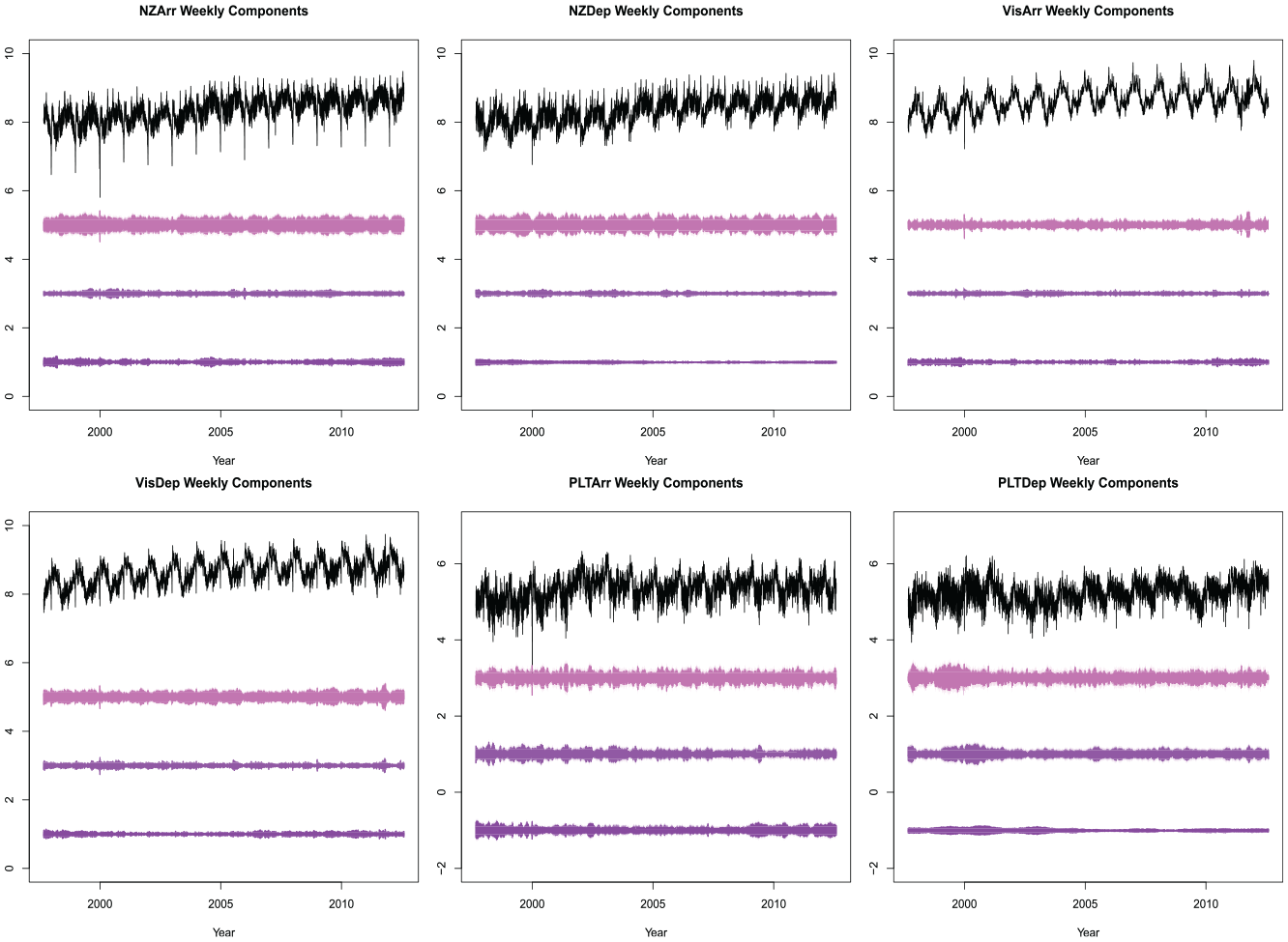
Weekly components for daily immigration data. Top pink line is the estimated once per week effect
6. Conclusion
In this manuscript we provide a new computational technique that expands the practical applicability of difference stationary latent component models. This flexible class of models can be used for a wide range of applications, including multivariate signal extraction. At the present time, estimating parameters with ML estimation has proven numerically infeasible for even moderate-dimensional problems. In this paper we improve upon the available computational methods by deriving an EM algorithm with an explicit formula for the M-step. This derivation allows for the white noise covariance matrix to be computed from a knowledge of the extracted signal and error covariances. Moreover, the formula is fast to compute (no matrix inversions), and hence the speed of the algorithm is only bounded by the numerical efficiency of a particular implementation of signal extraction (e.g., by SS or ES methods). This new methodology renders feasible the fitting of a six-dimensional daily time series, which previously was intractable.
Before this EM method for parameter estimation can be used in the production of official statistics, a number of important issues should be resolved. Firstly, fixed effects such as outliers and moving holiday effects need to be estimated concurrently with the time series model parameters; we suggest an iterative approach (as is used in modeling software such as X-13ARIMA-SEATS), whereby fixed effects are first estimated using regression (e.g., by generalized least squares) and subtracted from the data, followed by the EM iterations, and with this two-step dance repeated unto convergence. These fixed effects could be specified through univariate regressors, which is probably better than a multivariate approach when considering extreme values and holiday/calendrical phenomena. Secondly, the differencing polynomial needs to be identified as a crucial aspect of the time series model specification; this could be pursued in a univariate manner, assuming that the differencing polynomials are scalar, perhaps along the lines of model identification used in X-13ARIMA-SEATS. Thirdly, missing data (with potential ragged edges) should be integrated into the proposed algorithm, although this is already possible in ES; ES; McElroy (2022) discusses how ragged edge missing values can be accommodated in likelihood and signal extraction calculations, and such algorithms have been implemented (McElroy and Livsey 2022). Fourthly, as log transformations are commonly used in the analysis of time series data in official statistics, it is of interest to modify seasonal adjustments restated in the original data scale so as to be compatible with annual averages—this might be done by incorporating the proposed methods with benchmarking techniques.
This paper is focused on computation and applications, but does not delve deeply into the specifics of difference-stationary latent component models. The impact and applicability of such models can be greatly extended with the aid of the results presented in the manuscript. Moreover, our results can facilitate a hybrid estimation procedure, wherein EM is run for a few iterations, followed by a likelihood-based estimation that is initialized at those parameter estimates. Currently the latent component covariance matrices
Footnotes
Funding
The author(s) declared that they received no financial support for the research, authorship, and/or publication of this article.
Disclaimer
This report is released to inform interested parties of research and to encourage discussion. The views expressed on statistical issues are those of the authors and not those of the U.S. Census Bureau.
Received: September 2023
Accepted: June 2024