
Abstract
Errors in household finance survey data collection can lead to inaccuracies in population estimates. Manual case-by-case revision has traditionally been used to identify and edit potential errors and omissions in the data, such as omitted or misreported assets, income, and debts. Selective editing strategies aim at reducing the editing burden by prioritizing cases through a scoring function. However, the application of traditional selective editing strategies to household finance survey data is challenging due to their underlying assumptions. Using data from the Spanish Survey of Household Finances, we develop a machine learning approach to classify data during the editing phase into cases affected by severe errors and omissions. We compare the performance of several supervised classification algorithms and find that a Gradient Boosting Trees classifier outperforms the competitors. We then use the resulting score to prioritize cases and consider data editing efforts into the choice of an optimal classification threshold.
1. Introduction
Under the Total Survey Error Framework, the job of the survey designer is to minimize error throughout the survey lifecycle (Groves 2009). In addition to errors related to representation issues (e.g., sampling and nonresponse errors), measurement errors can also bias estimates of population parameters. The sequential process of detecting and correcting measurement error is often referred to as data editing (De Waal et al. 2011). Typically, statistical agencies and survey practitioners allocate a significant portion of their resources to manually detect these errors. In this context, selective editing emerges as a strategy to limit and prioritize manual editing (De Waal 2013). By implementing an optimized editing strategy statistical offices and researchers can save time and resources (Granquist and Kovar 1997).
A selective editing strategy involves fitting a score function to divide data into two streams: the critical stream (data records to be edited manually or interactively) and the noncritical stream (data records that do not require edits). To fit a score function, the seminal papers of Hidiroglou and Berthelot (1986) and Latouche and Berthelot (1992) propose to first predict an “anticipated value” using auxiliary variables for each unit-variable pair to construct scores. However, such anticipated value models present several challenges. First, they often rely on strong assumptions, such as using values from previous past data as a proxy for the anticipated value. Second, these models have not been tested within household finance surveys or surveys whose main output are highly skewed population distributions or contain a longitudinal component.
In this paper, we present a new selective editing application by using data from the Spanish Survey of Household Finances (EFF by its Spanish acronym) and a machine learning approach. We train a machine learning score function with a rich dataset from the 2017 and 2020 waves of the EFF. We also exploit text data from interviewers’ comments and clarifications introduced during the interview which, to our knowledge, have not been exploited in the literature. Using the estimated score, we separate cases into critical and noncritical stream groups, taking also into account manual editing costs. Finally, we evaluate the prediction power of the model using out-of-sample data not observed during the training phase, that is, the subsequent 2022 EFF wave.
The data editing process in the EFF survey is conducted interactively and presents two main features. First, as stated in Barceló et al. (2020), manual editing spans several months, hence, reducing the time devoted to it may produce economic savings. Automatic data editing methodologies alleviate some of the costs, through the identification of demographic inconsistencies which are easy to program and identify. However, the detection of other type of likely errors such as omissions, implausible values or inconsistencies is much harder to program exhaustively and requires manual editing intervention. This is a challenge for data production because errors may propagate and affect several variables along the interview given the complexity of the questionnaire. Kennickell (2017) documents the reasons why the production of household finance survey data is more challenging compared to, for instance, business surveys. A second feature regarding the interactive nature of the editing process is that households are sometimes recontacted in order to correct for potentially major errors, inconsistencies or omissions in the data, increasing the respondent burden. This may lead to the occurrence of break-off, which can affect data quality and survey inference (Peytchev 2009). Our goal is to prioritize editing by predicting potential recontacts, thereby reducing both the respondent and editing burden. The prediction of such characteristic resembles the recovery of the influential error probability of cases. By estimating the probability of recontact, we can divide cases into the critical and noncritical stream using a calculated optimal threshold. We state the main challenges encountered and compare the methodology against other selective editing methodologies. We also compare our threshold selection methodology and its optimal value against other methods of computing the optimal cutoff for dividing cases into two streams. Finally, we interpret the results of the machine learning model by using SHAP values, a novel framework that disentangles the main drivers of the scoring function.
The paper is organized as follows. In Section 2, we provide a literature review on selective editing methodologies and the usage of machine learning techniques in survey methodology. Section 3 motivates the present case study within the EFF framework. Section 4 describes the data and methodology used to approximate the recontact score function and the threshold selection methodology. In Section 5, we present and discuss the results. We also briefly discuss the main features, caveats, and extrapolations of this methodology in Section 6. Finally, in Section 7 we conclude and comment on future research.
2. Background
Survey data editing is often time-consuming and costly and takes a substantial part of the data production process (De Waal 2013). In household finance surveys, automatic data editing methodologies alleviate some of the costs, such as the identification of demographic inconsistencies which are easy to program and identify. However, the detection of other type of errors, such as omissions, implausible values or inconsistencies, is much harder to program exhaustively. Measurement errors may propagate due to the complexity of the questionnaire and this represents a challenge for the data production process. Errors in highly skewed data have the potential to create serious distortions in the measurement of wealth distribution (Kennickell 2006; Vermeulen 2018). Thus, on top of feasible automatized processes, manual case-by-case revision has been so far applied in the EFF in order to identify and correct potential errors and omissions.
So far, the available selective editing strategies in the literature focus on prioritizing cases based on their influence on some expected result. To measure influence, the survey practitioner must have a sense of the true value to be edited, that is, anticipated value. The anticipated value is used to construct the score that divides the sample into two groups: the critical and the noncritical streams. An anticipated value model can rely on a past value such as one coming from a previous survey edition (Hidiroglou and Berthelot 1986). For example, it may be estimated from the mean or median of the target variable in a homogeneous subgroup of similar units from a previous period (Latouche and Berthelot 1992).
After constructing the score, the survey practitioner should determine the cutoff value to divide data records into the editing group (critical stream) and the non-editing group (noncritical stream). In order to do so, the researcher determines the effect of a range of threshold values on the bias in the estimated parameters of the principal survey population. Survey methodologists have proposed variations to this framework over time (Allard et al. 2001; Arbués et al. 2013; Gismondi 2007; Hedlin 2003; Zhu and Godbout 2011). The literature tested selective editing strategies in establishment, business, and census survey data. However, it is not trivial to define what constitutes an influential error in household finance surveys (Kennickell 2006). In this later context, predicting the probability of occurrence and the possible size of influential errors seems promising.
In this paper, we introduce the application of machine learning models in the selective editing literature. A machine learning algorithm is referred to as supervised when it is trained based on a target value that is known for, at least, some part of the data, which also enhances model evaluation. When a classifier is trained on such a dataset, the aim is also to tune the parameters of the model in order to devise a classification algorithm that would work well in future data. In this setup, there is no prior knowledge on which supervised machine learning model would perform better, thus, one has to compare several classifiers. The set of algorithms includes classical machine learning models such as Logistic Regression with regularization, K-Nearest Neighbors (KNN), Support Vector Machines (SVM), and well-known tree-based algorithms like Random Forests and Gradient Boosting Trees (XGBoost).
Recently, the application of machine learning techniques in survey methods research has become more widespread. There is new research in forecasting panel attrition (Kern et al. 2021), modeling unit non-response (Kern et al. 2019, 2021; Toth and Phipps 2014), identifying errors in textual data (He and Schonlau 2021), classifying coding errors (Schierholz and Schonlau 2020), and imputing data (Dagdoug et al. 2021) have emerged. In general, these techniques are becoming increasingly important in the survey data production process. To our knowledge, we are the first to apply machine learning techniques into the selective editing literature. In this sense, we also contribute to the survey methodology literature by providing an empirical use case where we produce scores that allow for edit prioritization. Our selective editing approach prioritizes cases based on their likelihood of substantial errors and omissions that need to be corrected through the recontact with the respondent, rather than solely with respect to certain expected results from the data. Thus, this paper speaks to the micro-selection approach and, particularly, the prediction model approach. For a comprehensive review of this literature, refer to De Waal et al. (2011) and Granquist and Kovar (1997).
3. Case Study
The EFF is a longitudinal survey conducted by the Banco de España (BdE by its Spanish acronym), which provides detailed information on households’ assets, debt, income, and spending since 2002. The population frame for the EFF sample is the Continuous Population Register, where the units are households as defined by their postal addresses. The survey performs stratified sampling based on information from individual wealth and income tax returns categories held by the Spanish Tax Agency which are oversampled progressively. Most questions in the survey pertain to the household as a whole, except for labor and related income, which are specific to each household member over the age of 16. The majority of information refers to the time of the interview, although details on all pre-tax income sources also refer to the previous calendar year.
Data collection is carried out through personal interviews with households which are conducted by interviewers with specialized training and using computer-assisted personal interviewing (CAPI) methods. In 2020, due to the pandemic context, interviews were conducted by telephone (CATI). The EFF fieldwork typically spans around nine months, starting in October of the corresponding wave year. The final sample usually comprises around 6,300 households, with approximately 50% having participated in previous EFF waves (forming the panel component). Oversampling of wealthy individuals accounts for approximately 12% of the top 1% of the wealth distribution. The average response rate is about 40% for the non-panel component and 75% for the panel component. For a detailed overview of the survey characteristics, including response rates, sample sizes, and other EFF methodological details, please see Barceló et al. (2020) and visit the official website (https://app.bde.es/efs_www/home?lang=ES).
In order to train a supervised machine learning classification model, one needs a target variable that identifies the set of critical cases. In our use case, it is an indicator variable constructed from past waves editing records. Throughout the data production process, which begins immediately after the start of the fieldwork, numerous data quality control and validation tasks are conducted. In addition to many hard and soft checks performed by the CAPI to minimize various types of errors (such as values out of range, implausible values, and inconsistencies), BdE and the fieldwork company (FC) perform extensive manual editing of all completed interviews. Furthermore, interviewers’ work is closely supervised not only in terms of response rates but also in terms of data quality. As part of the data production, the data is edited by means of an iterative process with the FC, as outlined in Figure 1. During the initial stage, the editing team at the FC reviews all completed questionnaires, identifies potential errors, such as implausible values, coding errors, inconsistencies, monetary errors, and omitted information and introduces editions in the production system. Comments and clarifications entered during the interview by interviewers and audio records are useful throughout the process. Given the significant impact that major errors and omissions can have on the final data, the FC categorizes cases affected by severe potential errors which cannot be solved with the available information—distinguishing between priority cases and non-priority cases. Then, the team at BdE conducts a second revision of the priority cases. It’s worth noting that BdE also revises many non-priority interviews from interviewers requiring close monitoring at the beginning of the fieldwork to provide feedback and correct any interviewer protocol or conceptual mistakes, although these do not need to a priority case. In cases where the BdE’s revision of a priority case confirms potential errors or omissions that cannot be solved with the available information, the BdE requests the survey agency to recontact the household to clarify responses and collect important omitted information.
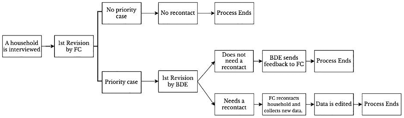
Recontact process in the EFF.
The recontact consists of a phone call to the household respondent to conduct a shorter questionnaire focused on the aspects that need revision or correction. The EFF carefully considers the trade-off between obtaining additional information and potentially bothering households on a case-by-case basis. One of the advantages of recontacting households is the considerable reduction in the overall measurement error of the survey. Additionally, it enhances the representativeness of the sample, as fewer cases/questionnaires need to be discarded. The types of omissions that typically lead to a recontact include unreported labor status, omitted income, real estate assets or debts, incorrect valuation of businesses, and errors in household composition, among others.
Once the editing finishes, the data comes to a imputation process that produces multiple alternative values to correct for item non-responses (Barceló et al. 2020), including missing values generated in the editing phase. Thus, data editing affects imputation results.
4. Data and Methods
In this section, we describe the dependent variable along with the auxiliary dataset employed for training and fitting the models. Then, we explain the methodology used to train the models and the criteria employed to select the best training model. We elucidate the process of selecting an optimal cutoff or threshold value for dividing cases into the critical and noncritical streams. Finally, we discuss the interpretability of our preferred model and evaluate the results using out-of-sample data.
4.1. Data
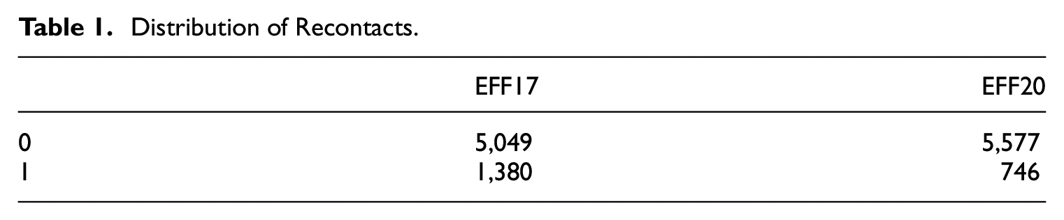
We use raw data and editing files from the EFF 2017 and 2020 waves. As explained in Section 3, we train the models with a dependent dichotomous variable that takes value 1 when a case had substantial potential errors or omissions that implied a recontact, and 0 otherwise. Table 1 presents the distribution of the dependent variable in each wave.
Distribution of Recontacts.
Records from previous waves were executed by different editing teams, thus, the dependent variable is not exempt from measurement error. Classification errors may be a burden to train a model and predict with accuracy. In particular, changes to revision and classification procedures across waves may compromise the usefulness of the dependent variable. However, in Subsection 5.4 we provide a series of performance and validation metrics which support predictability and out-of-sample validity of the model. In addition, there were instances where the editing team did not reach households requiring a recontact or households did not want to answer. Thus, we re-train the model taking into account those instances and show that the predictability of the model is slightly worse. One could think that a model based only on cases where values were corrected during recontact would be more interesting. However, in the EFF, cases where households do not answer the recontact are also edited when they present inconsistencies, while the solution might be assigning missing values to the inconsistent variables. Of course, this might be specific of the EFF where there is imputation of missing data. In addition, it is difficult to disentangle which value change is due to the recontact or the standard revision of a case in a successful recontact. We also study the relationship of prediction errors with ex-post editing information. We deal with these issues in Subsection 5.5.
The explanatory variables are drawn from multiple datasets, primarily questionnaire responses, paradata, and metadata. Table 2 provides a description of each set of inputs and Table A1 in the Appendix contains descriptive statistics for selected variables. Based on the experience from EFF reviewers, household financial characteristics usually offer valuable insights into identifying data problems, for example, households with complex financial structures are more likely to necessitate follow-up contact. In addition, interviewers with less experience and training in conducting complex surveys tend to produce lower-quality interviews. Research by Bristle et al. (2019) indicates that interviewer characteristics, such as education level and experience, may serve as good predictors of panel cooperation. Interviewers may also influence household responses (Durrant et al. 2010; Flores-Macias and Lawson 2008). Furthermore, paradata, such as the time taken to answer a question, may offer insights into data quality (Groves and Heeringa 2006). Our set of predictors encompasses both household and interviewer-generated data and characteristics.
Description of Explanatory Variables.
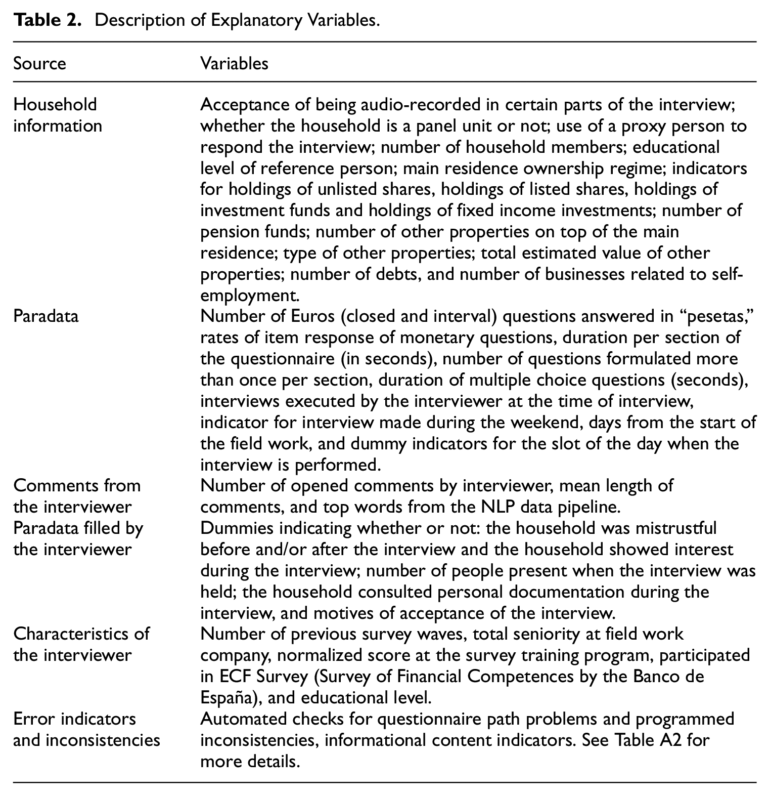
We include household data for questions formulated to every household but also information that the editing team acknowledges was relevant in the manual identification of recontact cases. Additionally, we exploit text data from interviewers’ comments and clarifications introduced during the interview with the CAPI software, a novel source of data that, to our knowledge, has not been exploited in the literature. Such comments are useful in the editing process as they help to decide whether a question has been answered well or there is some error. We parse the comments with pre-trained models from Honnibal et al. (2020), removing stopwords, punctuation signs, alpha numeric characters, and others. Then, we apply Porter (2001) stemming and produce word counts under a bag-of-words approach. Finally, we select those words that are more present in each class (top twenty words with highest relative importance within that class). After running several experiments, we found that the extra complexity of other models based on TF-IDF counts (Sammut and Webb 2010), did not improve the out-of-sample performance of the model. We also generate other set of predictors from the text as described in Table 2. Lastly, we incorporate a set of automated indicators for errors and inconsistencies that have been used automatically identify some errors in the data, see Table A2 of the Appendix for details. We also apply mean centering to the variables that change levels across waves, these are, the obtained interviewer evaluation score during the interviewers training and duration of questions in seconds. The reason for the latter is that the EFF2020 was performed using a CATI collection mode due to the pandemic. Overall, our set of predictors consists of approximately 275 variables.
4.2. Training and Evaluation
We compare a set of classical machine learning models, Logistic Regression with regularization, K-Nearest Neighbors (KNN), Support Vector Machines (SVM), and the well-known tree-based algorithms—Random Forests and Gradient Boosting Trees (XGBoost). The algorithmic capability increases in the aforementioned list, from simple linear models to non-linear and flexible algorithms that exhibit improved performance in higher dimensional settings. The use of bootstrap aggregation techniques with decision trees, also known as random forests, has recently gained popularity in the survey research community (see Buskirk (2018) for more details). Although neural networks may be a viable option, the literature suggests that boosting and bagging techniques outperform neural net algorithms in applications using structured data (Borisov et al. 2024).
In order to overcome the relatively small sample size of a test set, we design a three-step process of training and evaluation to compare the models. To reduce the potential bias introduced by seed initialization in splitting the training and test sets, we perform the following three steps on ten different seeds and average the results:
We proportionally randomly split the dataset into 70% train and 30% test sets by keeping the share of critical cases of the full sample in every partition.
We fit the model with a five-fold stratified cross-validation strategy for hyperparameter tuning in the training data. The cross-validation aims to minimize the log-loss function or negative log-likelihood for binary data:

where p is the probability of being the critical class, y is observed target variable, and log is the logarithmic expression.
3. We evaluate the performance of the model by computing evaluation metrics in the test data.
In the process of training a machine learning algorithm, it’s necessary to split the dataset to evaluate the classifier’s performance (Step 1). Step 2 involves fitting a given classifier to the data. To accomplish this, a cross-validation strategy is used to optimize the classifier’s configuration by tuning its hyperparameters. We employed a grid search optimization algorithm for the first three classifiers (i.e., the Logistic Regression Classifier, SVMs, and K-NN), and a random search algorithm with a maximum of 2,500 iterations for the Random Forest and Gradient Boosting Classifier. The tree-based algorithms explore spaces that generate at least 15,000 hyperparameter combinations. Therefore, randomly exploring a fifth of these possibilities seems more than sufficient to avoid falling into a suboptimal local space. In Table A3 we provide details about the hyperparameter strategies, along with their hyperparameter space and search methods. We explored a wide range of hyperparameters, and after numerous experiments, we determined that the hyperparameters listed in Table A3 were suitable representations of both suboptimal and optimal spaces for each model. It has been established that in a high-dimensional hyperparameter space, random search is a better approach than a grid search (Bergstra and Bengio 2012).
In Step 3, we assess the performance of the classifiers using two evaluation metrics averaged across the ten random seeds. The Receiver Operating Characteristic Area Under the Curve (ROC AUC) serves to evaluate the performance of binary classification models. It measures the model’s ability to distinguish between positive and negative classes by plotting the true positive (TP) rate against the false positive (FP) rate at different classification thresholds and computing the area under the resulting curve. The score ranges from 1, indicating perfect classification, to 0, with a score of 0.5 indicating that the model is no better than random classification. The ROC AUC score is insensitive to imbalanced datasets, which is the case for this application. Thus, we also use a second metric, the area under the curve (AUC) of the precision-recall curve. The precision-recall curve plots the proportion of true positive classifications among all positive classifications (precision) against the proportion of true positive classifications among all actual positives (recall). Again, the AUC of the precision-recall curve ranges from 0 to 1, with a higher value indicating better performance. The precision-recall curve focuses on the positive class and is more informative in cases where recall is more important than precision. This is the case in our application, as the increase in false negative cases can lead to higher measurement error in the final data, while the increase in false positive cases increases the revision time.
A comparison of the present use case against other selective editing use cases is worth noting. Our goal is to classify cases into recontact or not, that is, to predict a binary variable. This is distinct from other scoring models based on anticipated values that often predict a continuous variable. Additionally, the output of our use case produces a global score for each case. While in the selective editing literature, scores are often computed variable-by-variable and then aggregated at a global level for the whole survey sample (Lawrence and McKenzie 2000).
We also provide an out-of-sample evaluation of each model using data from wave 2022. This allows us to compare the predictions of the best trained model with the most recent manual classification made by the editing team. For that matter, the final score (or predicted probability of a household to be recontacted) is the median across the ten fitted classifiers scores, as if one were inferring within a production environment. The reason to use the median in this context is twofold. First, it is better to provide a single metric to the editing team as opposed to scores for every seed in order to generate an efficient process of prioritization. Second, the median is robust to outliers coming from potential data drifts in new data, that is, changes in the data generation process from unseen and incoming new questionnaires.
Finally, the computation of the models was implemented in Python (version 3.9) and the main machine learning packages utilized were scikit-learn (Pedregosa et al. 2011) for all algorithms, training, and validation; and xgboost (Chen and Guestrin 2016) for the extreme gradient boosting algorithm. The Python codes for the computation of the results are available through the Github repository https://github.com/nicoforteza/eff_score.
4.3. Optimal Threshold
Once we choose the best-fitted classifier, we have to select the optimal threshold that classifies cases into the critical and noncritical streams. Given the data imbalance, a 50% threshold would not make sense since the predicted probability distribution is left-skewed. On the other hand, there is a trade-off: increasing the threshold results in a lower false positive (FP) rate but an increasing false negative (FN) rate. False positives make the review team allocate additional time and resources to revise a case that does not contain substantial errors or inconsistencies. False negatives imply there would be left cases with substantial errors or omissions. Let precision be the proportion of true positive classifications among all positive classifications and let recall be the proportion of true positive classifications among all actual positives. In our setup, maximizing recall is relatively more important than maximizing precision, that is, maximizing the detection of positives while loosing precision at some degree due to increasing false positives. Thus, our approach let the researcher choose the importance of recall relative to precision rather than an arbitrary threshold or cut-off. The performance metric we use is the F β score of precision and recall,
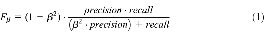
where β is the importance of recall with respect to precision. The maximization of such evaluation metric provides an optimal threshold.
5. Results
This section presents the resulting performance metrics of the different classification models that are used in order to select the best classifier. For the best model, we present optimal thresholds as a function of the value β chosen by the researcher or statistician. We interpret the results of the model by showing the most important variables and how they relate to the prediction outcomes. In addition, we validate the predictability of the model in new out-of-sample data. Finally, we provide additional robustness analysis.
5.1. Best Model
As shown in Figure 2, the KNN classifier and SVM classifier are the worst performers among the competing algorithms, with XGBoost, random forest, and logistic classifier with Lasso regularization being the best performers, both in terms of AUC-ROC and PR-AUC scores. This result supports the use of ensemble and tree-based algorithms in tabular data, in line with Kern et al. (2019). XGBoost, with its boosting feature, outperforms all other algorithms. The fact that the metrics for PR-AUC are generally lower than those for AUC-ROC means that the algorithm’s ability to detect positives (questionnaires masking multiple omissions, errors, etc.) is lower than its ability to differentiate between the two classes.
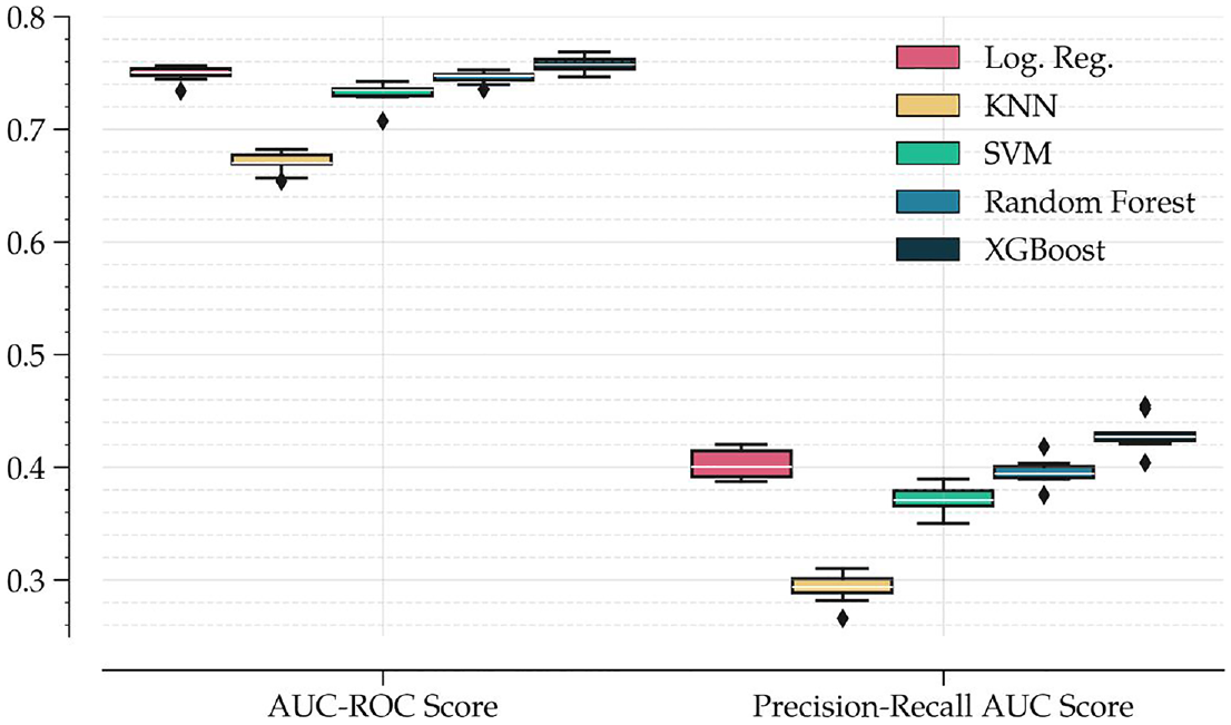
Classifiers performance metrics.
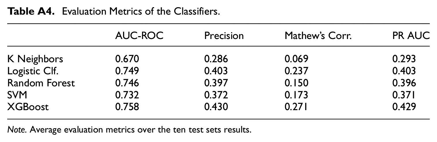
Table A4 of the Appendix presents average evaluation metrics across the ten seeds. In general, achieving high levels across performance metrics is challenging. The fact that the ROC curve presents a level of 0.75 already implies that the model’s prediction is 50% better than that of a fully random model or, alternatively, that it is 25% lower than a perfect fit model. The closest reference in the literature to which we may compare our results is Kern et al. (2021); however, this application faces a different classification task and dataset. In our use case, the data generation process depends on the extensive depth of the logical tree of the questionnaire. This implies significant heterogeneity and variability in the data, what is a challenge for any model to be able to generalize across multiple test sets. In our data, no two cases are the same in the entire sample. In fact, the number of variables collected throughout the survey amounts to more than 7,500, exceeding the number of observations. Additionally, interviewers and data editors introduce further heterogeneity in the data generation process which we analyze in Subsection 5.5.2.
5.2. Optimal Threshold
Table 3 presents, for different values of βs, the resulting precision, recall and F β values. For a full simulated grid of βs and corresponding F β values, please see Figure B1. Note that a higher value of F β score does not necessarily imply a better performance of the model, the relative importance assigned to occurrence of false negatives matters for a conclusion, that is, cases that conceal important errors or omissions that the model fails to detect. For instance, in a setup where optimizing recall is more important than optimizing precision, β equal to 1.5, the resulting optimal threshold is estimated to be approximately 0.14. This implies that the team would assign cases with a score above 0.14 to the critical stream, which amounts to 40.1% of the sample.
Optimal Thresholds for a Set βs.
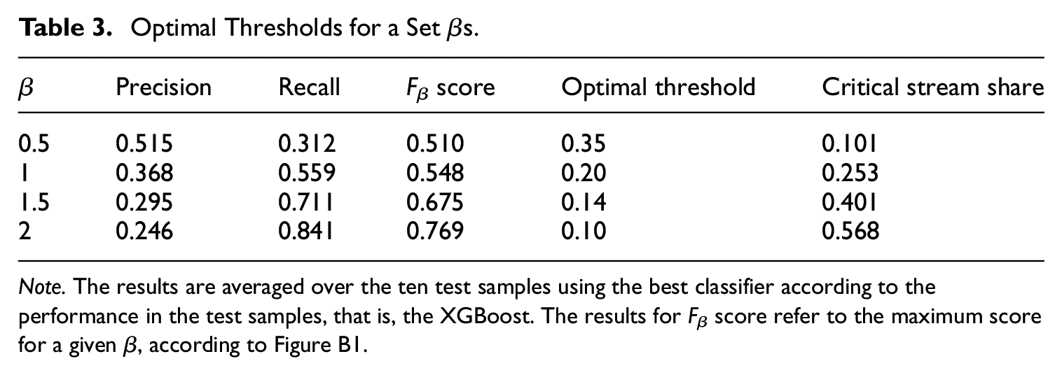
Note. The results are averaged over the ten test samples using the best classifier according to the performance in the test samples, that is, the XGBoost. The results for F β score refer to the maximum score for a given β, according to Figure B1.
By looking at Figure 3, one can observe the main implications of choosing different thresholds. The higher the score, the more precise the model is, that is, a higher share of true positives for each bin. This means that sorting the completed interviews according to the score yields a list of cases by their likelihood of recontact, with a decreasing chance of entailing important errors as the score decreases. Furthermore, as one reduces the threshold, the number of false negatives increases, while increasing the threshold may end up in under-editing, where population parameters could be contaminated due to insufficient resources allocated to editing efforts. The score is a tool for the editing team in order to prioritize editing. In the previous example, for a threshold of 0.14, according to Figure 3 the editing team would revise a total of 3,826 cases: 1,688 would be true negatives, 521 true positives, 1,502 false positives, and 115 false negatives. The associated recall and precision for the seed used in Figure 3 are 0.82 and 0.26, respectively.
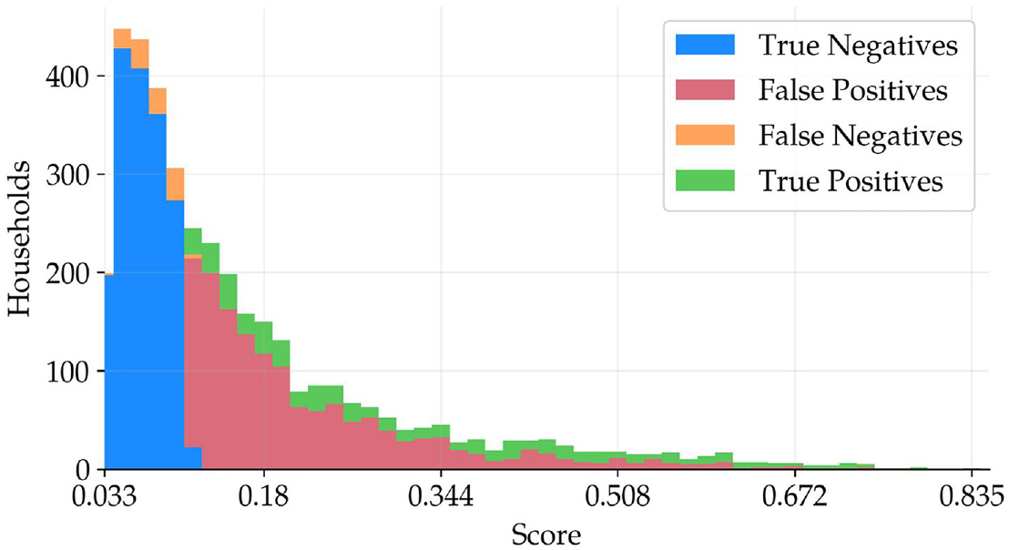
Distribution of a cross-tabulation of predictions against true values.
5.3. Interpretability
One of the main drawbacks of using ensemble and tree-based algorithms is their complex interpretability. According to Miller (2019), interpretability of a machine learning model refers to the degree to which a human can understand the cause of a decision made by the model. To interpret what factors or variables drive the score, we use the SHAP (SHapley Additive exPlanations) framework developed by Lundberg and Lee (2017). The SHAP value measures the impact of a variable on the model’s prediction. The machine learning model’s prediction can be represented as the sum of its computed SHAP values, plus a fixed base value.
Figure 4a shows the most influential variables in the classification model according to the mean absolute value of their SHAP values. The most important variable is “days from start of the fieldwork.” The second most important variable is an indicator for errors in the employment situation of any member in the household. However, these results do not inform about the direction of the relationship between the variables and the outcome, for example, are early interviews in the fieldwork more or less prone to recontact? Figure 4b is a beeswarm plot of the SHAP values for the top eleventh variables according to their mean absolute SHAP values as in Figure 4a. For each variable, it shows the distribution of estimated SHAP values, each dot is a SHAP value which is mapped to the associated variable’s value; the lighter the dot, the higher the variable value as indicated by the right-hand-side axis. A large and positive SHAP value indicates that the predicted probability of the critical class increases. For example, the top row displays the impact of the variable “Days from the start of fieldwork.” A darker color indicate lower values of the variable which, in this case, means interviews made earlier in the field work; yellow and light green state for higher values which mean interviews made later in the field work. Thus, interviews made earlier in the field work tend to have a positive impact in the probability of being of the recontact class. Interviewers are more prone to making mistakes at the beginning of the fieldwork, and the data editors tend to find more cases that require a recontact during this time. The dispersion among SHAP values means that the impact of the covariates’ value on predicting the critical class is heterogeneous. For instance, for the binary variable “employment situation error,” the impact of positive values is different for each household and this is because it depends on the interaction with other variables. The number of questions about financial assets and businesses, which is larger if the household hold more of such assets, is the third most important variable, which implies that the higher the financial and businesses complexity, the greater the probability of being recontacted. This is also the case for the duration of the set of questions on businesses and financial assets, which confirms that wealth complexity positively relates to the probability of being the critical class. The larger the number of completed interviews made by an interviewer at the time of an interview, the lower the probability of being the critical class. The interviewer experience and training score are also very important variables which are negatively related to the probability of being the critical class. The results align well with informal reviewer team expertise on the manual classification of cases into the critical class. In addition, an additional output that the application may provide is a report about SHAP values on a case-by-case bases. This report may guide the revision process for the critical set, potentially further improving the efficiency of the revision exercise. However, it is up to the reviewer team to evaluate whether this kind of guidance improves or worsens efficiency.
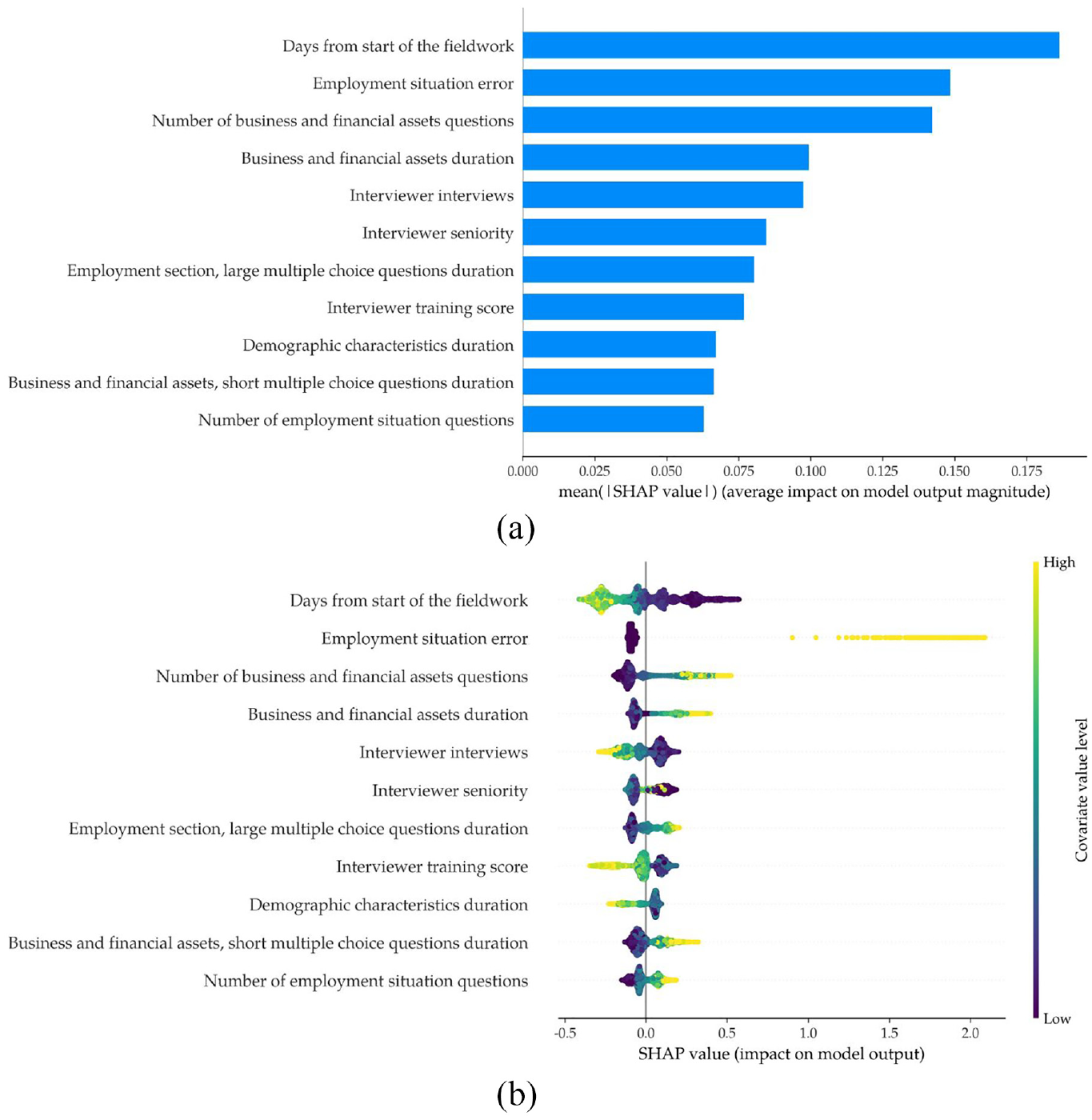
SHAP values for top variables: (a) highest SHAP values and (b) beeswarm plot of SHAP values.
5.4. Validation with EFF2022 Field Data
We also validate the model in out-of-sample data from EFF2022, that is, this data was not used either for training or testing the model. The sample size is 6,338 observations. Table 4 presents performance metrics for the three main ML classifiers which are the result of comparing the predictions of each model to the actual manual classification made in EFF2022. The results indicate that the model generalizes well based on the observed out-of-sample metrics. The ROC AUC score of 0.73 indicates that the fitted classifier does not overfit and can consistently make predictions on new generated data (out-of-sample).The PR AUC is lower in the validation exercise than in the baseline, however, the reader should note that this metric is sensitive to data imbalances. In particular, in the validation exercise the recontact rate is 10% while in the baseline is 16.5%. The relative increase in false positives in the EFF2022 predictions affects precision which, together with the fact that there is a lower rate of recontacts, decreases PR AUC. In contrast, the ROC AUC accounts for the rate of false positives and false negatives equally, the ROC AUC remains almost unchanged, which suggests the model maintains its discriminative power across thresholds. It is important to note that there may be changes to the questionnaire, editing techniques and guidelines in new waves. The editing team also varies in terms of composition and experience, potentially affecting the manual case-by-case classification of cases into recontacts. Thus, differences between in-sample and out-of-sample evaluation metrics can be expected. Nonetheless, the results indicate that the prediction tool is reliable across waves.
Evaluation Over EFF2022.
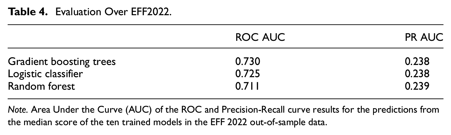
Note. Area Under the Curve (AUC) of the ROC and Precision-Recall curve results for the predictions from the median score of the ten trained models in the EFF 2022 out-of-sample data.
5.5. Additional Robustness
To address potential concerns regarding the relevance of the outcome, we present an analysis based on an alternative outcome variable, which incorporates ex-post information on the success or failure of a recontact. Additionally, we explore the unexplained variance of the model.
5.5.1. Successful Recontacts
Recontacts can fail if the household respondent does not want to answer any more questions or if households do not pick the phone. The purpose of this exercise is to demonstrate the validity and robustness of the classification model when using only cases that were effectively recontacted. It also may be the case that a researcher is only interested in applying the classifier to those kind of cases. Thus, we construct an alternative indicator for realized or successful recontacts, which we use as dependent variable. A share of 89% of recontacts were successful between 2017 and 2020. We retrain the classification model and evaluate the steps, as outlined in Subsection 4.1, using this alternative target variable. Table 5 reports average performance metrics in the test samples of three different algorithms trained with data of successful recontacts. The performance is worse than that of the baseline classifier; the PR AUC and ROC AUC of XGBoost are 0.39 and 0.75, respectively, while that of the baseline model were 0.42 and 0.76. On top of the better performance of the baseline classifier, an agile implementation of the score increases the likelihood of a successful recontact, hence it makes more sense to implement a model for all kind of recontacts.
Performance Metrics for Classification of Successful Recontacts.
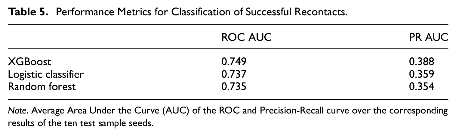
Note. Average Area Under the Curve (AUC) of the ROC and Precision-Recall curve over the corresponding results of the ten test sample seeds.
5.5.2. Error Analysis
While we include hundreds of explanatory variables in the prediction model, there are still prediction errors. In this section, we analyze in which degree factors that cannot be used for prediction, but are available at the end of collecting and editing the data of each wave, relate to the propensity of being the critical class or not. To do so, we regress the log-loss prediction errors for the entire training sample on interviewer, regional, reviewer or/and wave dummies, depending on the specification.
In Table 6, we present how adjusted R2 varies under different specifications. Interviewer effects explain 4.5% of the variation in log-loss errors while reviewer effects explain 15.7% of it. Wave effects do not play a role once taking into account interviewer and reviewer effects. An interpretation of the results is that the classification model is not capable of achieving better performance because there are interviewer and reviewer effects that explain part of recontact classification, for example, the reviewer team while doing the manual classification into the critical class in past data introduced reviewer effects and there are interviewer effects on top of all interviewer controls used included in the model. However, these factors are unobservable and cannot be used for prediction. Manual classification tasks usually carry human bias. A machine learning model which could incorporate reviewer and interviewer effects would enhance performance metrics and reduce prediction errors. However, this is out of the scope of this paper.
Error Decomposition of the Predictions.
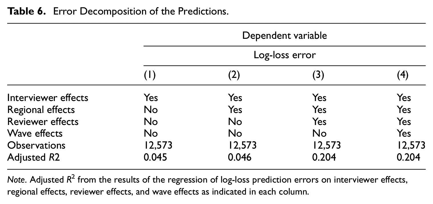
Note. Adjusted R2 from the results of the regression of log-loss prediction errors on interviewer effects, regional effects, reviewer effects, and wave effects as indicated in each column.
6. Discussion
There are several differences between our use case and other score function approaches. Firstly, our method relies on a more flexible approach, as we do not impose any restrictions on the score function for dividing cases into critical and noncritical streams. In addition, anticipated value models seem not suitable for household finance data with a panel component because the financial situation of households (and their composition) varies over time. In the absence of an anticipated value, one cannot disentangle the score into risk and influence factors. Our threshold selection emphasizes resource allocation for interactive editing rather than the impact of editing a subset of records on survey population estimates.
Overall, our proposed methods can be adopted in other financial household surveys which can profit from revision flags indicating problematic cases and a sufficiently large sample. However, incorporating human knowledge within a machine learning training procedure is crucial to obtain interpretable and desired results.
The EFF is currently under pilot implementation of the score function estimated in this paper. There are some challenges in order to do this. First, input and output data files have to be harmonized in order to design an automatization procedure to track cases across the field work stage. Second, it requires the coordination between the FC and the editing team at BdE to efficiently exploit the score together with other revision tools. Finally, it also requires the development of user-friendly documentation and visualization tools in order to describe and report the score, how to use it properly and interpret associated data, as SHAP values.
A main drawback for future practitioners willing to implement this procedure is the lack of an analysis accounting for the impact of selective editing on population parameters. To make an evaluation of the effects of editing, it would be necessary to impute missing values in alternative versions of the data, and potentially even having to reweight the cases in some instances. This analysis is out of the scope of this paper. However, there are simulation studies that measure the extent of the impact of a particular threshold selection methodology on population estimates, or that compute an optimal threshold value as described in Hidiroglou and Berthelot (1986). Data editing alters the set of information used in imputing missing value, however, Kennickell (2015) performed an exercise using the Survey of Consumer Finances (SCF), the results support a selective approach to editing and indicate that any resulting contamination of imputation is relatively minor.
7. Conclusion
We develop a novel application of machine learning in survey methodology that applies to the editing process of the EFF. We look for the best predictive model for detecting cases with substantial errors and omissions in raw data from questionnaires. By leveraging on revision data from previous waves, we train the models and show that tree-based ensemble models outperform other models in predicting substantial errors in the data. The resulting score function assigns a probability of being the critical class to each questionnaire given a large set of covariates. We show that the predictions align well with manual classification in different test sets. As part of our application, we also provide a tool to determine the optimal probability threshold to classify cases into the critical class taking into account the relative importance of recall versus precision for the predictions, that is, the share of false negatives relative to false positives that the statistical office or survey responsibles tolerate.
This application may provide an efficiency improvement for the survey and help reallocating resources. For example, the free-up of resources may help understanding other sources of error and feeding back to future questionnaire revisions and interviewer training. Our application may be useful for survey practitioners, in particular, with surveys that can exploit information from previous revision and editing processes. The approach is especially useful in cases where there is limited funding preventing massive manual revision.
Our paper opens several venues for future research. First, the use of audio features collected during the survey could enrich the auxiliary dataset, as these features have demonstrated usefulness in survey methodology and in manual revision. Second, quantifying the impact of the score on the final data would be enlightening, this is not a trivial exercise as discussed in this paper. Finally, it would be interesting to explore the usefulness of on-the-fly training of the models during the fieldwork, as it may enhance performance by incorporating more data.
Footnotes
Appendix A
Evaluation Metrics of the Classifiers.
| AUC-ROC | Precision | Mathew’s Corr. | PR AUC | |
|---|---|---|---|---|
| K Neighbors | 0.670 | 0.286 | 0.069 | 0.293 |
| Logistic Clf. | 0.749 | 0.403 | 0.237 | 0.403 |
| Random Forest | 0.746 | 0.397 | 0.150 | 0.396 |
| SVM | 0.732 | 0.372 | 0.173 | 0.371 |
| XGBoost | 0.758 | 0.430 | 0.271 | 0.429 |
Note. Average evaluation metrics over the ten test sets results.
Appendix B
Acknowledgements
We thank the incredible help of Paloma Urcelay and Younes Aberkan El Hajui, as well as the numerous helpful comments and suggestions made by Cristina Barceló, Olympia Bover, Laura Crespo, Carlos Gento, Ernesto Villanueva, and Arthur B. Kennickell as well as for the work of the Spanish Survey of Household Finance team, the one producing the data we use. We also thank seminar participants at the 2021 Big Data & Data Science online conference by the Centro de Estudios Monetarios Latinoamericanos (CEMLA), Banco de España, the 2023 Symposium of Data Science and Statistics by the American Statistical Association at St. Louis (Missouri), the 2023 FCSM Research and Policy Conference and Federal Reserve Bank for their invaluable comments.
Authors’ Note
The views expressed in this paper are our own and do not necessarily reflect the views of the Banco de España or the European System of Central Banks.
Funding
The author(s) received no financial support for the research, authorship, and/or publication of this article.
Received: March 2024
Accepted: November 2024