
Abstract
Published survey data often are delivered as estimates computed over an epoch of time. Customers may desire to obtain survey estimates corresponding to epochs, or time points, that differ from the published estimates. This “change of support” problem can be addressed through the use of continuous-time models of the underlying population process, while taking into account the sampling error that survey data is subject to. The application of a Continuous AutoRegressive Moving Average (CARMA) model is investigated as a tool to provide change of support applications, thereby allowing interpolation for published survey estimates. A simulation study provides comparisons of competing estimation methods, and a synthetically constructed data set is developed in order to elucidate real data applications. The proposed method can be successful for change of support problems, despite modeling challenges with the CARMA framework.
1. Introduction
Published survey data typically correspond to regions and time periods (or epochs) that a statistical office deems sufficient to guard against disclosure, while also providing sufficient quality for policy inferences (Janicki et al. 2022). For example, the American Community Survey (ACS) publishes data for geographies larger than 65,000 persons for one-year epochs; however, for sparsely populated regions and smaller geographies such as Census tracts, only the longer epochs of five-years are available (United States Census Bureau 2014). Demand from governmental stakeholders as well as the general public for population features measured at increasingly granular points in time and space continues to grow. In addition, users of survey data may require customized data publications for non-standard regions or epochs. For example, the Veterans Affairs (VA) utilizes the ACS data for its internal calculations, but requires epochs corresponding to September 30 of each given year (McElroy et al. 2019).
Whereas direct calculation of custom epoch estimates from ACS micro-data is possible, such estimates might fail to meet publication standards on estimation quality and data privacy; moreover, additional resources are required to compute such custom tabulations. The goal of this paper is to develop methodology for custom epoch estimates computed from publicly available data via continuous-time models; these models are straightforward to fit and apply, thereby keeping the resource burden low. Whereas McElroy, Pang, and Sheldon 2019 (henceforth MPS) addressed this problem of custom epoch estimation using the same strategy of continuous-time modeling, in this paper we utilize a richer class of continuous-time stochastic processes toward the end of improving the accuracy of interpolations required for customized estimation. In the same spirit as MPS, we isolate the temporal aspect of the problem—essentially ignoring the spatial features of ACS estimates—on the grounds of model simplicity, leaving spatio-temporal interpolation for future work.
The problem of custom epoch estimation can be framed as a “change of support” problem, as it is described in the spatial-temporal literature (Bradley et al. 2015, 2016). In our paper the change of support problem is approached with continuous-time modeling tools, offering an extension of MPS that generalizes the Fay-Herriot model (henceforth FH; see Fay and Herriot 1979; Rao and Molina 2015). Whereas the methodology of MPS involves an interpolation constraint that removed the impact of sampling error variability on interpolated values, in this paper this restriction is relaxed. Another contrast is that the underlying model of MPS was a Brownian Motion with linear drift, which enforces a simple trend structure on the data; however, a more flexible model class is given by the CARMA (Continuous AutoRegressive Moving Average) processes (with regression effects), which allows for more nuanced dynamics (such as business cycles and seasonality). In FH there is no temporal structure assumed; although there are extensions of FH to discrete time series structure, to our knowledge the only continuous-time analogue of the FH model is the Brownian Motion model of MPS, which reduces (as does our work) to the FH model when the continuous-time process is white noise.
CARMA processes are the stationary solutions to a linear stochastic differential equation; see Doob (1944), Jones (1981), Bergstrom (1983), and Brockwell (1995). The covariance structure for the stationary CARMA class is given by Brockwell (2000), with generalizations in Brockwell (2001, 2004, 2009), and Brockwell and Marquardt (2005). Chambers and Thornton (2012) shows that CARMA under regular sampling can be represented by discrete ARMA (AutoRegressive Moving Average) models, and Thornton and Chambers (2017) works with a mixture of stock and flow series and their discrete ARMA representations in the multivariate setting; see McElroy and Politis (2019) for background on ARMA processes and characteristic polynomials. These known covariance results are applied to obtain interpolation (or kriging) formulae used to generate this paper’s custom epoch flow estimates. However, our implementation of the CARMA model is restricted to first and second order Continuous AutoRegressions (CAR), as the parameterization of higher order CAR (and CARMA) remains a challenging problem.
The methodology of this paper treats the change of support problem for data observed over epochs, or subsets of time, expressed as averages of the population variable over the epoch; whereas in a spatial context such averages are referred to as “areal data,” in the econometric time series literature they are referred to as “flow data,” or “flows” for short; see Chambers and McGarry (2002) and Harvey and Trimbur (2003) for terminology and definitions. Whereas the flow structure involves an average, and therefore may not be appropriate for some variables, this is a common device for describing areal data (Bradley et al. 2017), and this formulation is adopted into our temporal framework. We remark that the continuous-time formulation allows us to interpolate to arbitrary time points; a discrete-time approach, in contrast, does not permit this fuller flexibility. Finally, the role of sampling error is vital, as the increased uncertainty associated with narrower epochs is important to communicate to users.
The rest of this paper is organized as follows: Section 2 discusses the framework of surveys collected over time. Hierarchical modeling and small domain techniques are also reviewed. The main innovation of the paper is the application of CARMA processes to a small domain setting (and how custom epoch inferences can be obtained); this is described in Section 3. Section 4 summarizes a series of simulation studies that address practical inference issues that arise from CARMA models, and Section 5 provides a specific application upon a non-public monthly test data set of the ACS. Section 6 provides conclusions. Supplemental S-1 contains technical results on covariance forms of points and epochs for Brownian motion and for CARMA models, Supplemental S-2 provides further detail on simulations studying a comparison of estimators, and Supplemental S-3 contains plots of a synthetic data simulation. All references originating from the supplemental data file are denoted by S-#.
2. Survey Framework and Small Domain Review
The modeling of survey data (i.e., characterizing the sampling distribution of estimates) in official statistics is a common practice within the small area literature. The term “small area” refers to a region (temporal or spatial) or categorization whose extent is so small that it contains few sampling units; hence, estimates constructed from such small areas (also called “small domains”) have high variability. Typically, the distribution of the survey statistic is modeled with a normal distribution, expressing the observed statistic as a true unknown mean plus a latent error, whose variance is obtained from the survey estimate of the statistic’s variance (or some other data-derived proxy). In the small area (or small domain) literature, small areas correspond to geographical regions; the most common model in this context is the FH model (Fay and Herriot 1979).
Supposing that

Note that the mean value is Y
i
, and σ
i
2 is the sampling variance. The survey variance estimator

Here τ2 > 0 is the variance of the regression errors, and

Assuming the parameters are known, we can use Bayes Theorem to obtain the conditional distribution for the estimand:

The unknowns
In the case that the domains are epochs, we can view the Y i as a time series, and some authors have developed time series models that generalize Equation (2); see Bell and Hillmer (1987) and Bell and Hillmer (1990). Tiller (1992) expresses this basic formulation in the state space framework. Similarly, Rao and Yu (1994) provides an extension of small area models to time series data, formulating a model that includes a temporal component while allowing for cross-sectional modeling. Ghosh et al. (1996) provides a Bayesian structural time series model with small area regression covariates. Pfefferman and Tiller (2006) and Pfefferman et al. (2014) provide state space models for small area estimation while involving benchmarking. Further citations and details can be found in Rao and Molina (2015). However, we emphasize that this literature (including the spatio-temporal work of Bradley et al. (2015)) is focused entirely upon discrete time series frameworks, which do not easily allow interpolation nor allow for varying epoch sizes; the integration of continuous-time processes into a survey framework has received little attention so far.
A few papers examine the uncertainty of the sampling variance’s sample-based estimator. You and Chapman (2006) applies a Bayesian small area model, approaching the sampling variance as if the sample variance estimator’s sampling distribution follows a
3. Custom Epoch Estimation
This section first describes the mathematical framework for temporal change of support, and secondly specializes to a discussion of CARMA processes, which is the main innovation of the paper. The third and fourth subsections further specialize to CAR processes of order 1 and 2, which are the only cases that are implemented so far.
3.1. Change of Support Problems for Continuous Time Processes
Cross-sectional surveys (such as the ACS) can represent either single time points (i.e., point domains) or time periods (i.e., epochs). Whereas classical sampling mechanisms (Lohr 2010) do not consider the flow of time, here a discussion of surveys collected over time is provided so that population estimands and their corresponding sample estimates are clearly delineated.
The ACS is a cross-sectional survey conducted by using a rolling monthly panel, and is produced on an annual basis. This survey produces one-year and five-year estimation products for various geographies (see United States Census Bureau 2023b). Single year ACS estimates represent larger geographies, whereas the five-year ACS estimates represent both these larger geographies as well as smaller geographies. Both products are assumed to represent their related epoch. The ACS is not the only survey that is assumed to represent an epoch; some governmental surveys report activity over an entire month (e.g., the Current Population Survey (United States Census Bureau 2022)), whereas many polls represent weeks or a few days (e.g., Gallup Research (Jones 2020)). In all of these cases there is a common need to express population parameters as an average over an epoch.
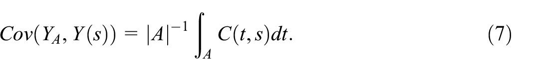
Surveys collected over time yield flow estimands computed over epochs that are dictated by the survey construction. A user may instead require an estimate for a different epoch than those being published; this is known as the “change of support” problem (Cressie 1993), and is similar to interpolation, where a continuous time model is needed to describe the data process at times that are not directly observed. As in the previous section, Y denotes a quantity of interest for the population, and this is viewed as a function of time t, denoted as

where |A| denotes the Lebesgue measure of A. (Most epochs of interest are intervals.)
The treatment of stock and flow is unified by recognizing that

where
Whereas the above expressions hold for a generic square integrable continuous time process, it is useful to assume that the population process
Two more practical modifications are made to the Gaussian process. First, note that

where row-vector
Applying the discussion in Section 2, the sampling distribution of the survey-based statistical estimates

where
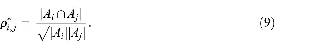
Such a formula for the correlation amounts to an unverifiable assumption to those external to the U.S. Census Bureau, and is indeed restrictive (as it presumes a lack of bunching in the data collection), but is arguably the simplest formulation in this context (it is also adopted in MPS; future research could investigate whether such an assumption is empirically sound). It follows that the covariance matrix of the sampling errors is defined by
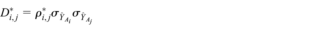
for

where
From the assumptions on the process
The covariance matrix of
for any t. In particular,

which will be used to estimate model parameters, and is the composition of survey error and continuous-time process error.
This treatment generalizes the FH model when epochs are disjoint and have equal length, that is,
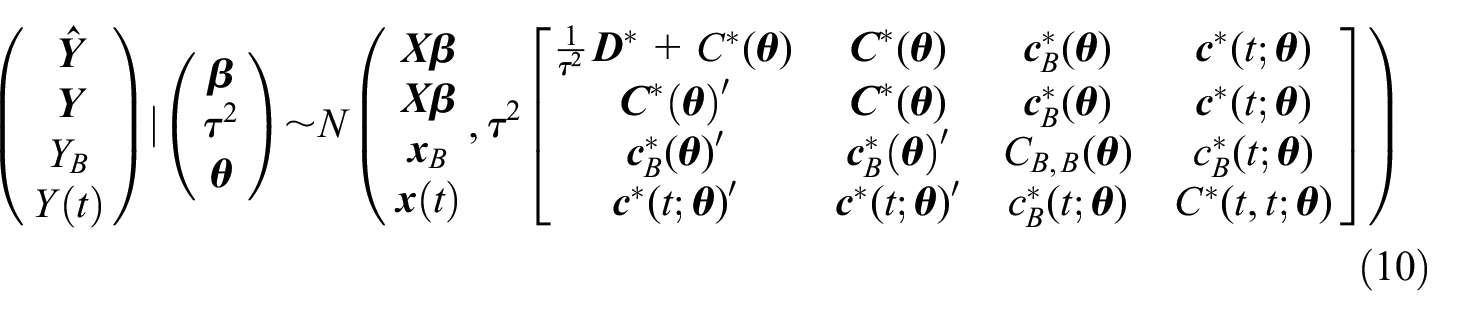
The problem of custom epoch estimation is to obtain the distribution of
Where

and


and

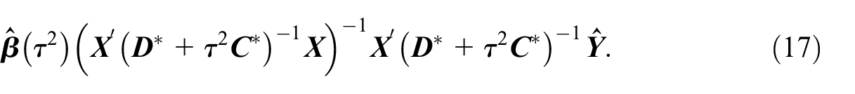
The estimation of the model form using Equation (11) and its likelihood, denoted
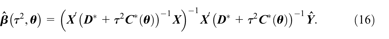
Plugging Equation (16) into the log likelihood, the desired solution is obtained by optimizing the result with respect to
3.2. Brownian Motion and CARMA as the Population Process
In the previous subsection
The use of continuous-time processes has a long history, especially in the domain of financial mathematics (Steele 2012 as an example). MPS proposed Brownian Motion to model the population process, addressing the problem of estimating
Further, τ2 can be obtained by optimizing a criterion discussed in MPS. A constraint on the interpolation estimator was also employed in MPS, but here it is preferred to instead use Equations (12) and (13).
For a standard Brownian Motion model,
The covariance structure of a mean zero stationary Gaussian process can be summarized through the spectral density
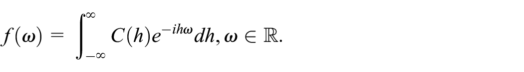
Here
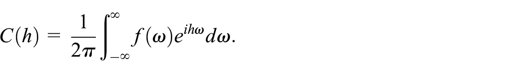
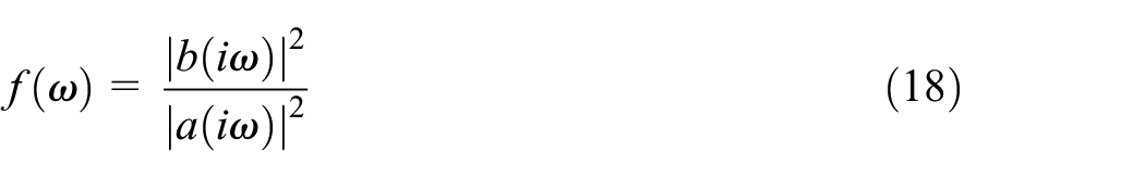
Hence, we can specify a zero-mean stationary Gaussian process by proposing an integrable non-negative function f for the spectral density; the CARMA class amounts to taking
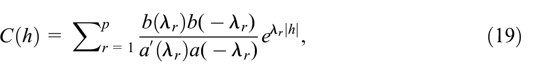
Specifically (following Brockwell (2000)), a zero-mean Gaussian process
for

(which is called the characteristic polynomial), and

where it is assumed that
where
It should be noted that there is no natural order to the roots of the polynomial
A similar issue afflicts discrete-time ARMA processes, where the stability constraint is concerned with whether the polynomial roots are outside the unit circle. Although in this discrete-time case the parameterization issue has been solved, it appears to be an open problem for CARMA; for this reason, we focus on CAR(1) and CAR(2) processes in our implementation. We remark that there are many connections between discrete-time ARMA and CARMA processes: Chan and Tong (1987), He and Wang (1989), and Brockwell and Brockwell (1999) establish that some ARMA models can be embedded into the CARMA framework. Conversely, regularly sampled CARMA processes become discrete-time ARMA processes, although this mapping is not surjective; see Chambers and Thornton (2012) for more details.
3.3. Special Cases of CARMA(1,0) and CARMA(2,0)
Here we develop the cases p = 1, 2 with q = 0 in greater detail. Beginning with p = 1 and q = 0, the single root λ must be real and negative, and the autocovariance function has formula

Hence,
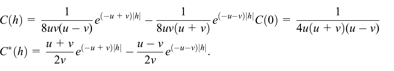
In the case of a CARMA(2,0) process, the roots λ1 and λ2 are either both real (and negative) or are complex conjugates (with negative real part). Conveniently, λ1, λ2 have negative real part if and only if a1, a2 > 0, which means that the space of positive coefficient quadratics has a simple parameterization, and the roots can be computed from the quadratic formula. (Such a property does not hold for higher degree polynomials.) Equivalently, the real roots can be written as −u ± v (0 < v < u) and complex conjugate roots as −u ± vi, where u,v∈ R+. (For repeated roots, we must allow v = 0.) The autocovariance and autocorrelation function in the case of two distinct real roots −u ± v is given by
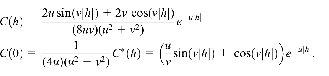
In the case of complex conjugate roots −u ± vi the autocovariances and autocorrelations are given by
For the double root solution of −u, an extension of (19)—see McElroy (2013) and Brockwell (2000), for example—yields

which is also the limit as
To illustrate the flexibility of the CARMA class we provide two graphical examples. First, we plot (see Figure 1) a stationary GP (this is the Gaussian kernel process described in Subsection 4.3 below) together with a CAR(1) process (dashed line), which tracks the simulation quite well; for purposes of illustration, we chose the parameters so as to facilitate a visual correspondence, and used the same random seeds. Also plotted is a simulated Brownian Motion (dotted line), whose trajectory reflects linearly growing variability. Clearly, Brownian Motion is not appropriate for the modeling of stationary data; in contrast, data with trend growth can possibly be modeled with a Brownian Motion, or by a CARMA model with linear trend regressor.
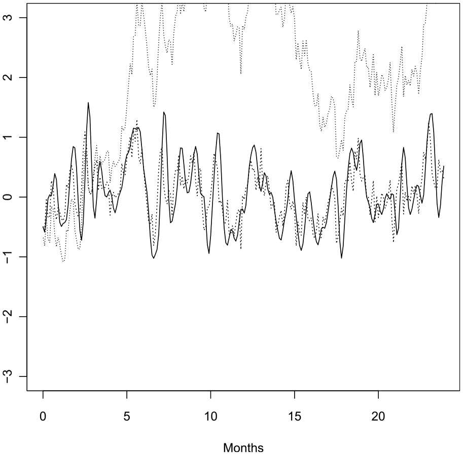
Simulation of a stationary process (solid line), a CAR(1) process (dashed line), and a Brownian Motion (dotted line). The basic time unit is a month, with ten observation times per month.
A second graphical example is displayed in Figure 2. The solid line is the same Gaussian kernel process added to a sinusoidal signal with a period of twelve months (or 120 observation times); the dash-dotted line is a CAR(2) process with complex conjugate roots
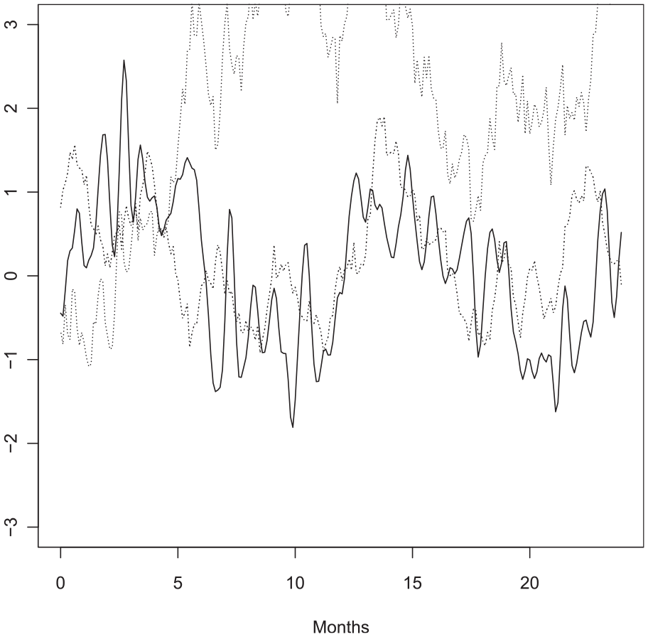
Simulation of a sinusoidal process (solid line), a CAR(2) process (dashed-dotted line), and a Brownian Motion (dotted line). The basic time unit is a month, with ten observation times per month.
3.4. Custom Epoch Inference Under the CARMA Model
Higher order CARMA models are capable of capturing much of the autocorrelation structure of an arbitrary stationary process, since the CARMA spectral density is a rational function of squared frequency—this is analogous to the ability of discrete ARMA models to describe a large class of stationary processes. The roots of the autoregressive characteristic polynomial can be associated with particular autocorrelation dynamics (or equivalently, peaks in the spectral density). Due to the challenges of parameterization we restrict ourselves to the p = 2, q = 0 setting for the remainder of this paper (note that the CAR(1) is a sub-model of the CAR(2)); although this may not be a sufficiently rich class of models to adequately capture all the features of the population process, we are able to obtain improvements over other methods (such as Brownian Motion) while maintaining simplicity of formulation and estimation. The implementation of higher order CARMA will require additional research into a flexible parameterization of the characteristic polynomial
To perform inferences for custom epochs using the CAR(2) model for the population process, the modeler must provide the data vector
Estimate an initial value of
Estimate initial CAR(2) parameters by computing
With
Optimization for obtaining τ0 was carried out via the Brent optimization method (Brent 1973). Optimizations for
The initializations delineated above are chosen due to the sensitivity of the likelihood to inputs. Because our methodology is designed to accommodate data with diverse epoch lengths, method of moments initializations (which rely upon regularly-sampled flow data) are unlikely to yield good results. Furthermore, this situation is exacerbated by the presence of unequal survey variance errors.
In order to estimate the parameters
hence if only one root equals
After the estimation procedures, the parameter estimates are inserted into Equations (12) and (14). Of specific interest toward estimation and model evaluation within this paper is the prediction of
4. Simulation Study
4.1. Simulation Setup
We assess through simulations the effectiveness of the CARMA process for modeling flow-observed survey estimates, and make comparisons with related models, viz. comparisons are made against a model based upon a mid-point observed CARMA with the same sampling error; against the Brownian Motion model of MPS both with strict restriction (as applied in MPS) and without; and against FH using flow CARMA as the true covariance function in Subsection 4.2, and using a Gaussian kernel covariance function as the true covariance function in Subsection 4.3. Although FH was not designed for temporal data, and can be expected to perform poorly, we include it as a baseline of comparison. While the methods (as well as the computer code) allow for overlapping epochs, the simulations focus upon non-overlapping scenarios—this mimics the intended ACS application. The restriction to non-overlapping flows implies that
Four configurations of parameters for the study are presented here. Four monthly flow epoch estimators and four continuous-time estimators are studied.
For each simulation three time series are generated, corresponding to ten years of monthly data (the units for the continuous-time process are months) for
This last series is meant to evaluate the continuous-time estimate.
–There are
–Each simulation involves the regressors
–There are three levels of survey error:
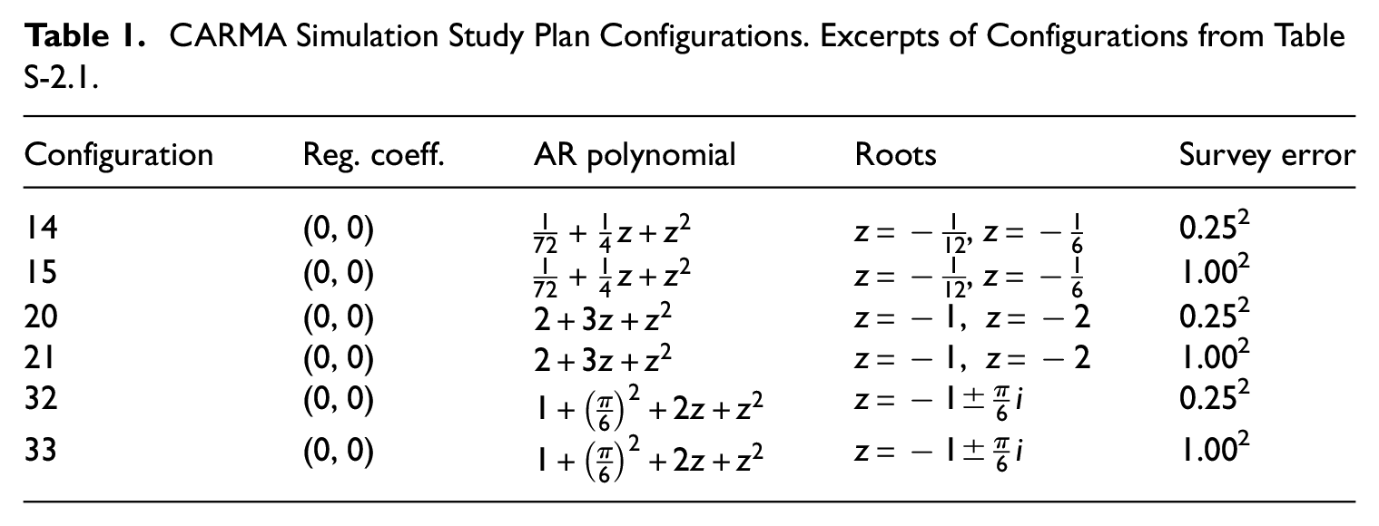
–There are six configurations of the CARMA characteristic polynomial: two representing a CAR(1) process and four representing CAR(2) processes. The latter case breaks into two cases of complex conjugate roots and two cases of a pair of real roots. Each pair of cases mentioned divides into two scenarios, namely a slowly decaying autocovariance function and a rapidly decaying autocovariance function. See Table S-2.1 for the complete configuration, and Table 1 for the shortened version.
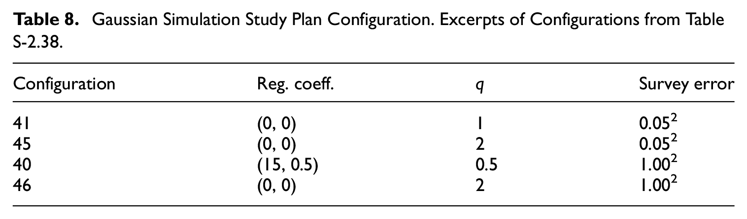
–There are three configurations of the Gaussian kernel scale parameter q, viz. q = 0.5, q = 1, and q = 2. See Table S-2.38 for the complete configuration, and Table 8 for the shortened version. Four models are used to estimate the small domains (via Equation (12) in the first three cases).
–M1 uses the flow-sampled CARMA process with survey error model.
–M2 uses the stock form of the CARMA process with survey error model, such that each survey estimate is assumed to have occurred at the center of the flow interval.
–M3 uses the flow-sampled Brownian Motion with survey error model.
–M4 uses the FH model. Four models are used to estimate the point domains (via Equation (14)).
–M1 uses the flow-sampled CARMA process with survey error.
–M2 uses the stock-sampled CARMA process with survey error model, such that each survey estimate is assumed to have occurred at the center of the flow interval.
–M3a uses the flow-sampled Brownian Motion with survey error model.
–M3b uses the flow-sampled Brownian Motion with survey error model, but also constrains each flow estimate to the exact value observed.
CARMA Simulation Study Plan Configurations. Excerpts of Configurations from Table S-2.1.
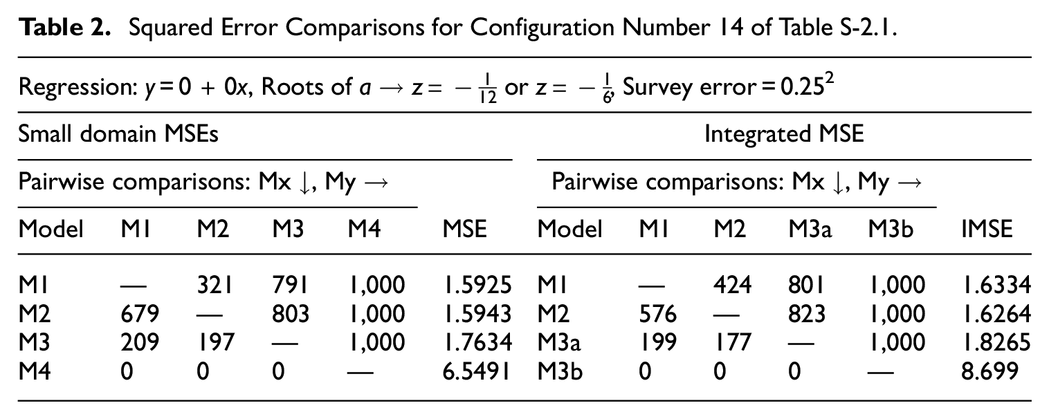
Small domain estimates are jointly compared by computing the sums of squares
4.2. Study: CARMA as Data Generating Process
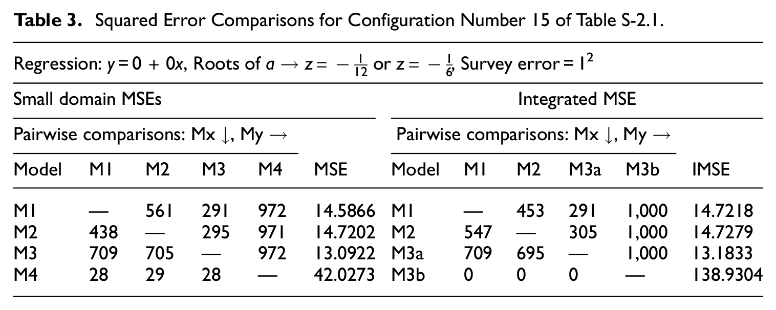
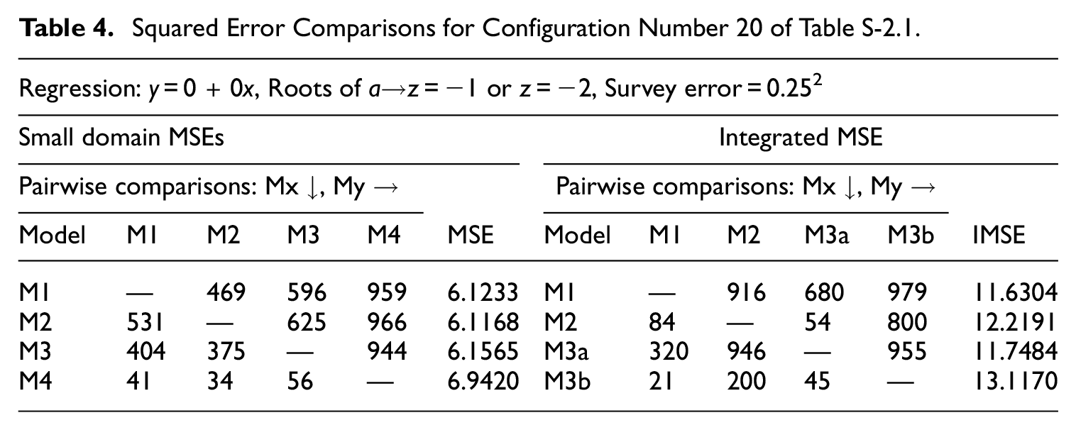
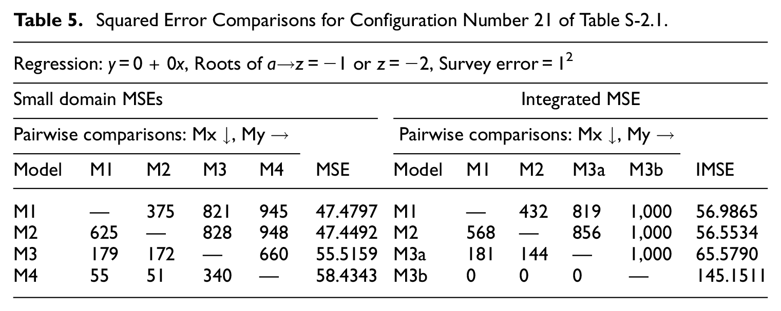
This section examines the performance of the models when the true data process is CARMA. A short list of the parameter configurations is given in Table 1. These excerpts, as given in Tables 2-7, focus upon the pair
Squared Error Comparisons for Configuration Number 14 of Table S-2.1.
Squared Error Comparisons for Configuration Number 15 of Table S-2.1.
Squared Error Comparisons for Configuration Number 20 of Table S-2.1.
Squared Error Comparisons for Configuration Number 21 of Table S-2.1.
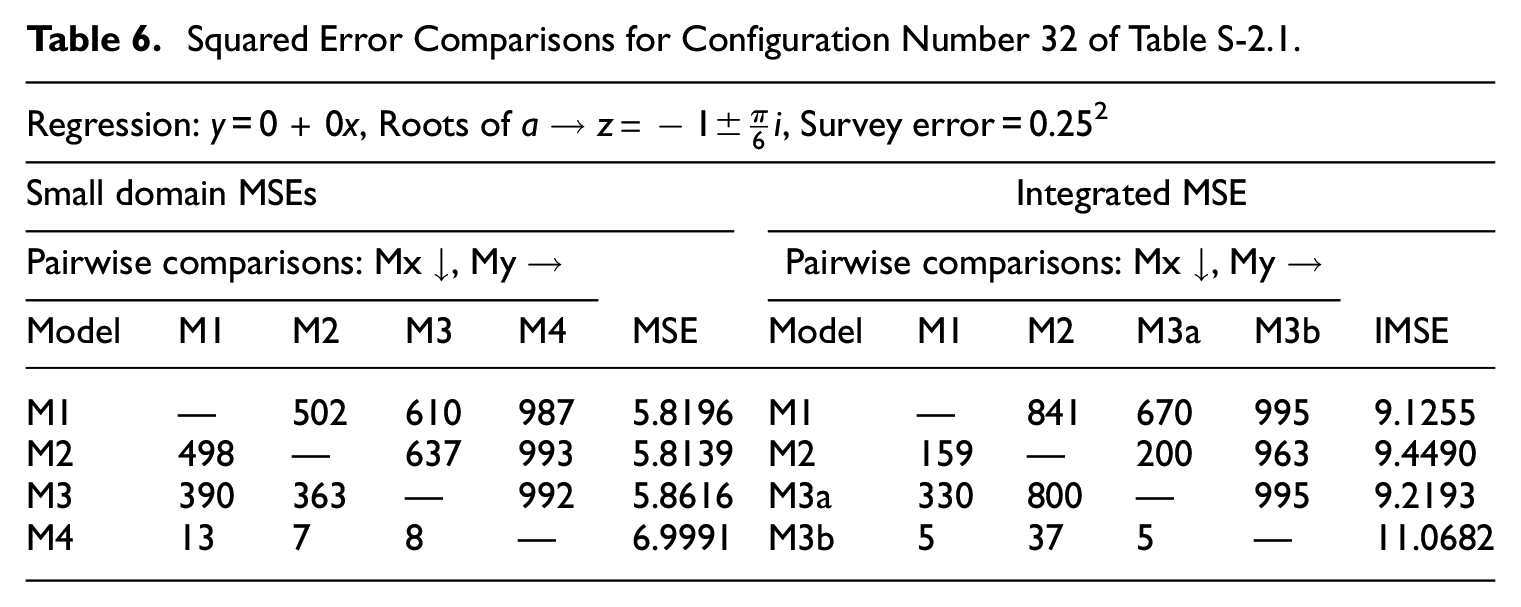
Squared Error Comparisons for Configuration Number 32 of Table S-2.1.
Squared Error Comparisons for Configuration Number 33 of Table S-2.1.
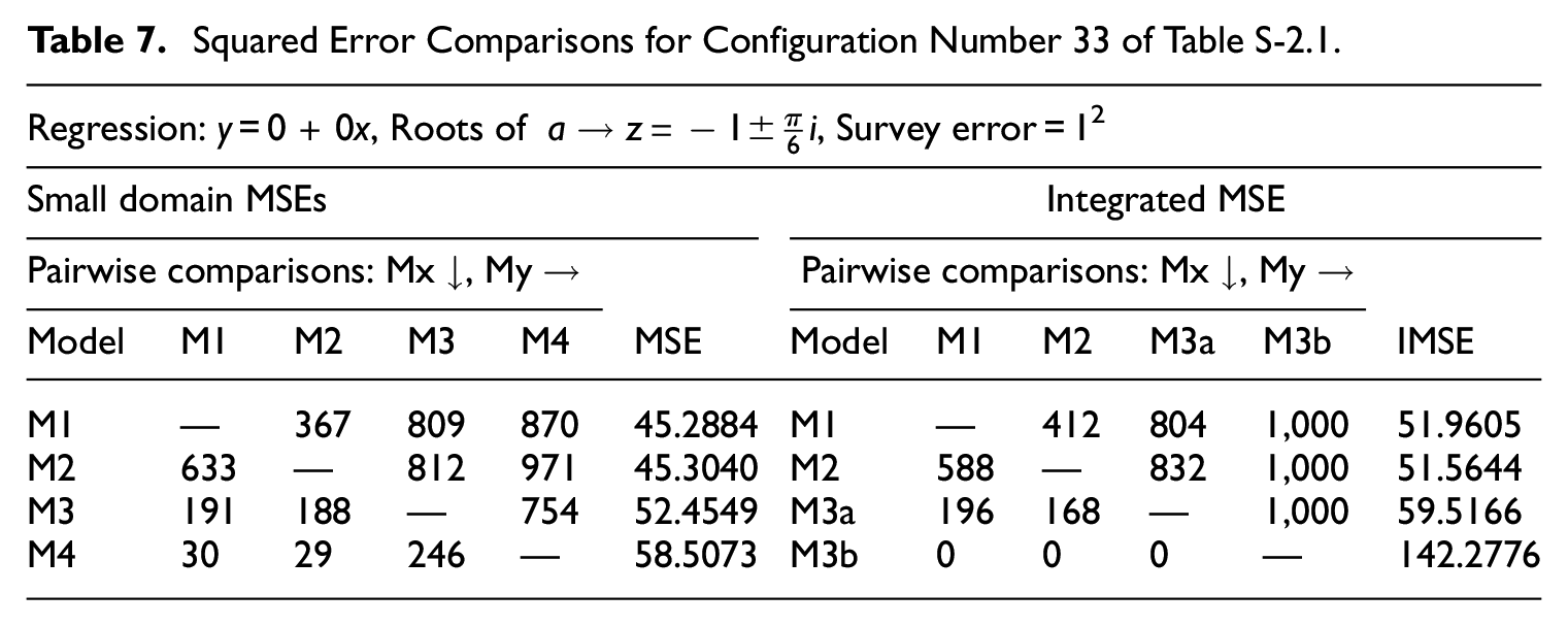
The main lesson of the simulation study is that the M1 (flow) and M2 (stock) models perform similarly in terms of monthly squared errors, and in some cases the stock model performs better upon flow-generated data. However, there are differences between M1 and M2 when comparing integrals of square errors when
4.3. Study: Gaussian Kernel as Data Generating Process
The Gaussian kernel process (see Supplement S-1.3 for the full definition) has covariance function
The Gaussian kernel process has strictly positive autocorrelations that decay more rapidly than the exponential rate of CARMA processes. Hence, Gaussian kernel and CARMA are distinct classes except in the trivial case that both correspond to a white noise (the limiting case of q tending to infinity); in particular, a CARMA model is always mis-specified for a Gaussian kernel process with q < ∞.
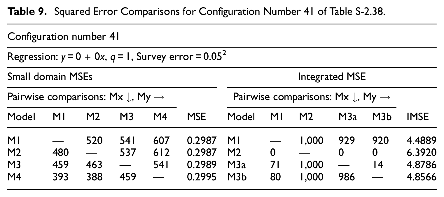
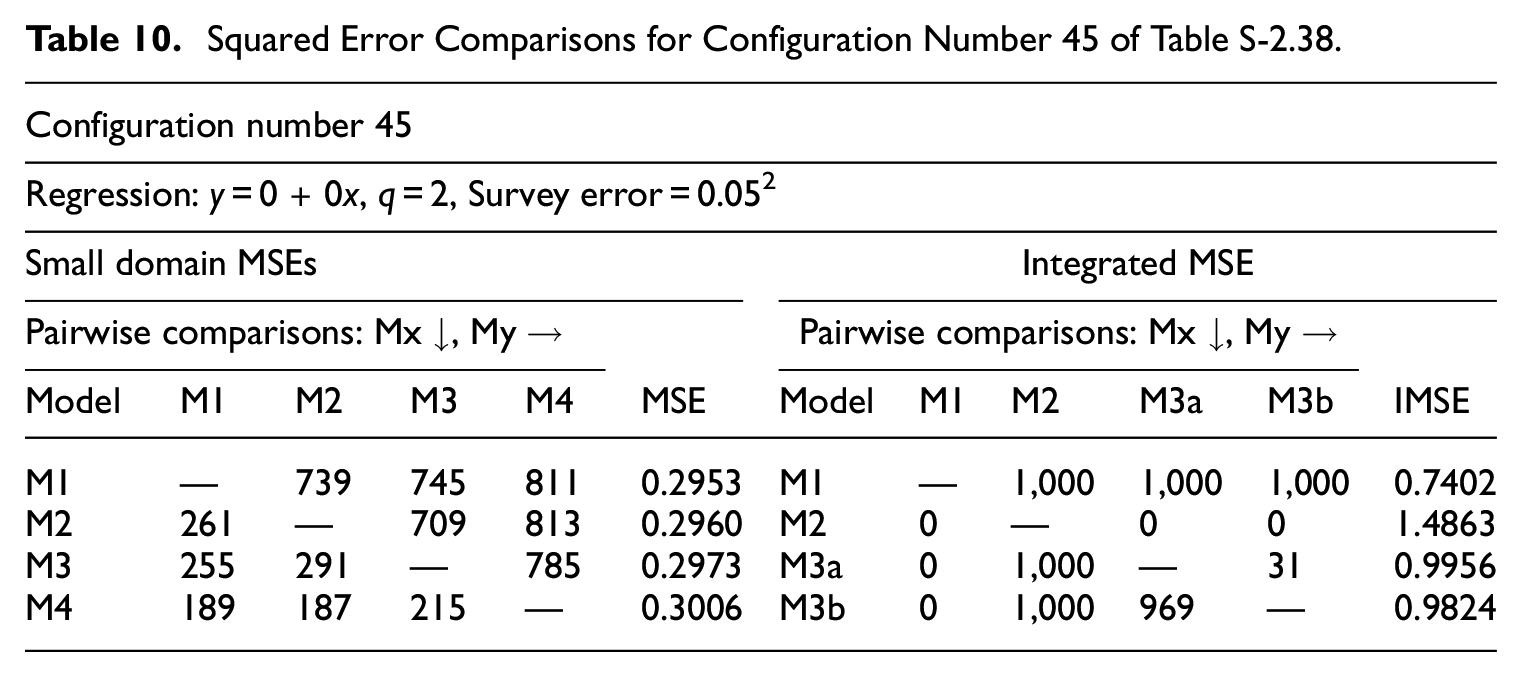
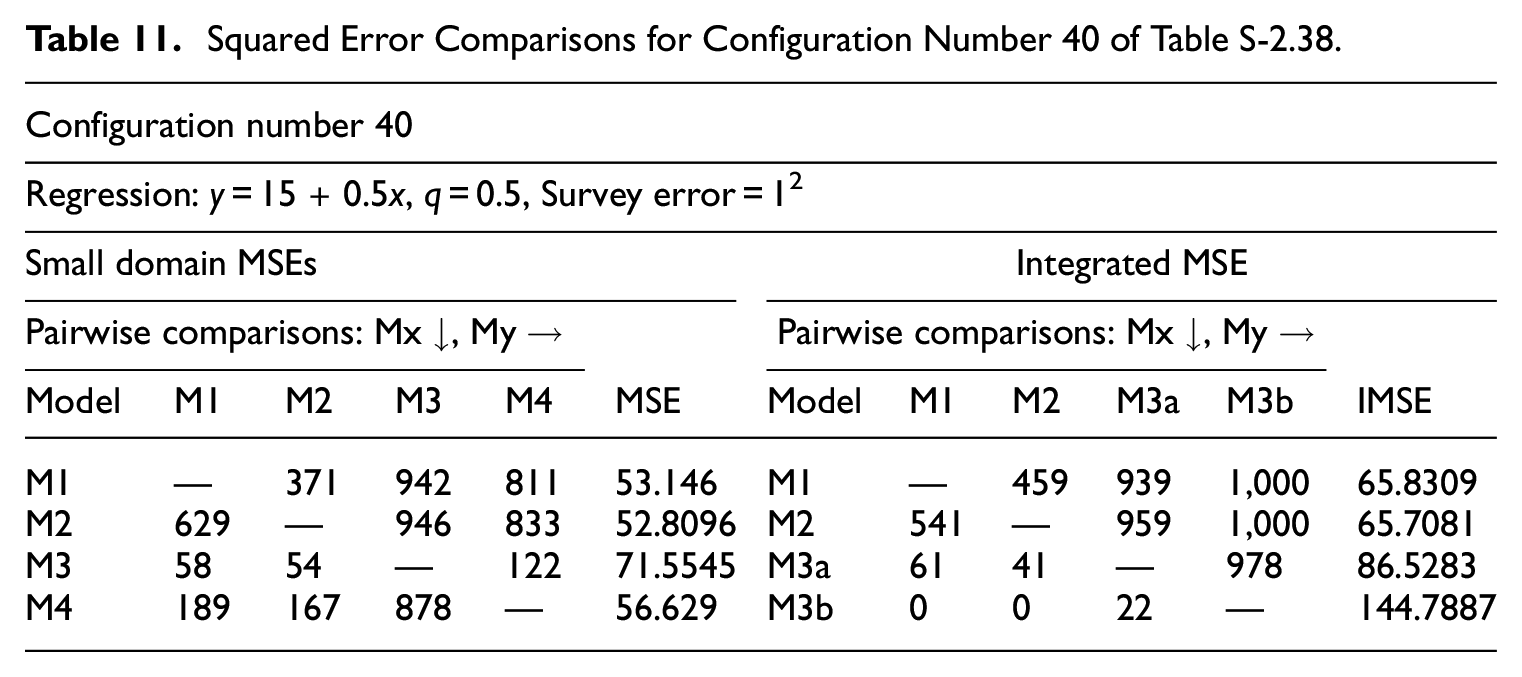
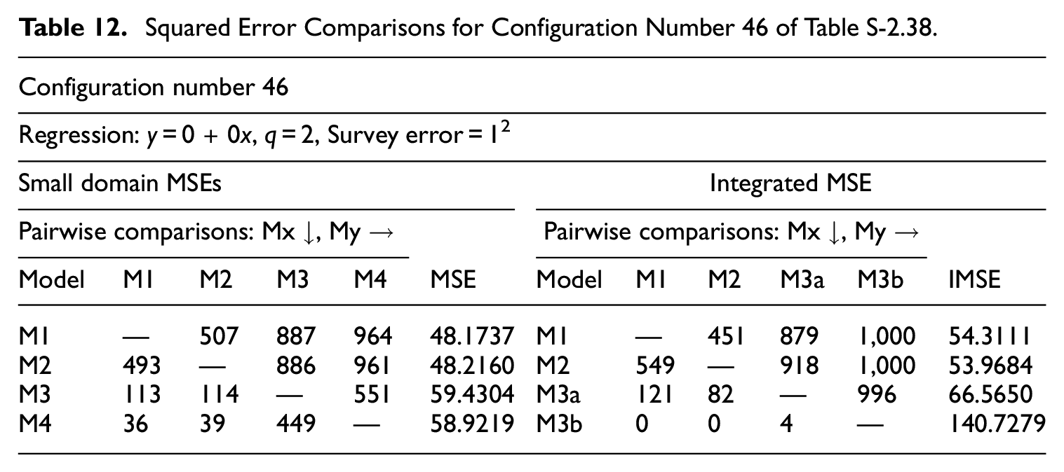
A short list of the parameter configurations is given in Table 8. A main feature, as demonstrated by Tables 9 and 10, is that M1 gives smaller small domain MSEs for some of the configurations when the survey error is small relative to model error; however, the results are inconclusive when comparing to M2. For cases where survey error and model error are at parity, M2 can exhibit smaller small domain MSEs than M1; moreover, M2 appears to have better integrated MSEs. Examples of this can be seen in Tables 11 and 12. Across all simulations, excepting where M2 has difficulties with extrapolation, the CARMA models perform better than the Brownian Motion (M3, M3a, M3b) and FH (M4) models.
Gaussian Simulation Study Plan Configuration. Excerpts of Configurations from Table S-2.38.
Squared Error Comparisons for Configuration Number 41 of Table S-2.38.
Squared Error Comparisons for Configuration Number 45 of Table S-2.38.
Squared Error Comparisons for Configuration Number 40 of Table S-2.38.
Squared Error Comparisons for Configuration Number 46 of Table S-2.38.
5. Application to ACS Data: Monthly Test Data
The ACS collects many requested and legally mandated questions from the American people, and is published annually at many levels of geographic aggregation. The survey produces one-year (single year) estimates for large geographies and five-year average estimates for smaller geographies. The survey is conducted on a monthly basis with multiple modes of response, along with follow-up for item non-response conducted annually for each calendar year the data is collected. The ACS weighting is calibrated such that totals computed across important demographic categories (such as Age-group, Sex, Race, and Hispanic origin) are enforced to equal independently constructed annual “Population Estimates,” with the matching performed using either the data-collection year for one-year ACS estimates or all years for the five-year estimate.
The purpose of this section is to exhibit properties of the model’s monthly and yearly estimates on a real data exercise consisting of monthly ACS data. Due to the difficulty of making such data public, the choice was made to create synthetic datasets in place of monthly ACS data. The method of constructing synthetic datasets is provided below, and then applied under different CARMA covariance parameter configurations. These datasets are then estimated under the model to demonstrate monthly and yearly shrinkage in variance.
5.1. Experiment on Missing Data Dealing with a Real Case
Monthly ACS estimates constitute a case of interest for the application of custom epoch estimation, as monthly estimates give a smaller temporal granularity than yearly estimates (which were explored in MPS). To explore the possibility of such a data product, the U.S. Census Bureau created an experimental dataset consisting of the observed household units for forty-nine states (omitting Alaska), along with the various survey weights for computing monthly estimates, as well as the survey responses. The steps taken to create this dataset are described in Albright and Asiala (2016) (additional discussion of sub-annual ACS estimates can be found in King (2010)). U.S. Census Bureau staff studied this dataset and determined that such monthly estimation methods would not meet the various quality standards for production (however, this dataset was made available for further time series research); in this paper we construct a synthetic monthly ACS dataset from published annual data.
One particular item of interest within the dataset is the question of the number of U.S. military veterans. The goal of MPS was to provide a method of sub-annual inference for U.S. military veterans using public ACS one-year, three-year, and/or five-year data for a specific date within the calendar year. This goal was addressed through modeling of the autocovariance structure of the time series data, thereby allowing for a change of domain. The present paper’s utilization of CARMA processes shares a similar goal to that of MPS, which was to estimate the number of U.S. military veterans. Here we examine a synthetic monthly dataset instead, whose longer time series sample length makes feasible our continuous-time modeling.
Although our primary interest is in assessing how the flow-sampled CARMA model performs in estimating monthly values, a secondary goal is to infer missing values in the dataset. On October 2013, due to lapse of appropriations the ACS was unable to be collected, and so this value is missing; we are interested in estimating this missing monthly flow as well. (Although the collection and processing of the survey was also disrupted for September and November of 2013, for simplicity it is assumed that the ACS was conducted without disruption from January 2005 to December 2015, excepting only October 2013.)
A drawback of using the monthly test dataset described in Albright and Asiala (2016) is that it is unavailable for public viewing, and hence any derived statistics cannot be readily published. Instead, similar datasets are constructed from annual public data available through the U.S. Census Bureau’s Application Programming Interface (API; United States Census Bureau 2023a). In terms of the variable of interest, we focus upon the population of veterans of at least twenty-five years of age, which is obtainable with margin of error from the API. (The U.S. Census Bureau no longer provides Veteran population ACS estimates to the public for specific ACS years.)
It is acknowledged that such a synthetic dataset will not exactly represent all the facets of a real monthly dataset, and therefore this data scenario is a simplification of reality. The constructed datasets explore different parametric values of the CARMA model in order to explore what may happen with real data.
There are two other differences in scope between the synthetic and real datasets: the former does not include Alaska, since the synthetic dataset was created for investigative purposes, and the different sampling rules in Alaska cause additional complication; secondly, the synthetic dataset does not include group quarters. The synthesis will implicitly include both populations, as it is derived from the entire national population.
5.2. Generating a Synthetic Dataset from ACS Public Data
The task is to generate a monthly (synthetic) dataset from ACS public data; however, a few more annotations are necessary before proceeding. The yearly dataset with estimates and 90% confidence intervals is displayed in Figure 3. A box is used to emphasize that this estimate is a flow, corresponding to an epoch; the horizontal extent of the box corresponds to the epoch (time interval), whereas the vertical extent of the box corresponds to the confidence interval. Note that there is a visible shift downward in the yearly data values as time progresses. The cause of this level-shift is known, owing mainly to a change in the survey measurement instrument—the question regarding veteran status changed in 2013. A level-shift regressor is used in the modeling of the trend. All further analysis is on a timeline shifted to initial time t = 0, and re-scaled so that the scale represents a single month.
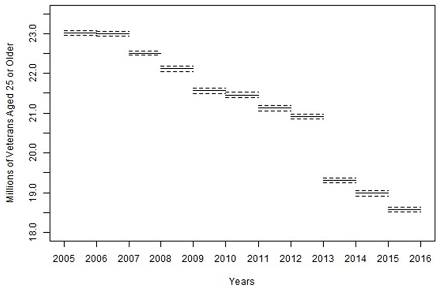
Plot of the one-year ACS estimates with 90% confidence margins of error for veterans aged twenty-five or older from 2005 to 2015.
A synthetic dataset D′ is constructed so that there are monthly estimates and related variances for those estimates, for each month from January 2005 to December 2015. The process of data construction starts with obtaining yearly sampling variances from public data; using that yearly public data with the base model Equation (11) to formulate parameter inputs for the monthly model (which are formed by assuming different values of CARMA parameters
There are three notations for time: t measures time continuously (in units of months), whereas m is a discrete index for the month, and j indexes the year. That is, let t = 0 correspond to the beginning of January 2005 and t = 132 correspond to the end of December 2015. Further, months are individually indexed
Construction of
Once yearly variances are obtained, synthetic model parameter values for
The next step is to generate monthly variances, followed by monthly observations. The monthly variances are defined by
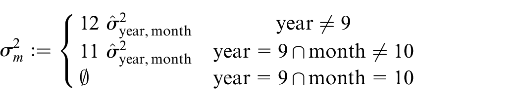
for years indexed as year =
Having created the synthetic model parameters based on yearly data and a choice of θ, and generated sampling variances for each month, the remaining task is to draw the synthetic monthly dataset from the public set. To do this, a conditional model for 132 monthly data points,
5.3. Applications of the Model to Veteran Status from Synthetic Data
The purpose of this subsection is to examine the capability of a CAR(2) model for generating custom monthly flow estimates. In particular, we are interested in whether the custom epoch variances (either Equation (13) for monthly epochs or Equation (15) for point domains) are less than the monthly sampling error variances, which would indicate a gain from using CARMA modeling. To examine this the synthetic data was run under six configurations of two root solutions. The first three configurations involve two real roots of a such that the roots of a are the pairs (−1/12, −1/6), (−1/4, −1/2), and (−2, −4). The second three configurations involve two imaginary roots of a such that the roots of a are pairs (−1/6 ± iπ/6), (−1/2 ± iπ/6), and (−2 ± iπ/6). Supplement S-3 contains a fuller discussion of these plots, but the analysis for the cases of (−1/12, −1/6), (−1/4, −1/2), (−1/6 ± iπ/6), and (−1/2 ± iπ/6) are similar to each other and to the analysis for the cases where (−2, −4) and (−2 ± iπ/6). As such, the cases for roots of a are (−1/12, −1/6) and (−2, −4) are given as examples.
Figures 4 and 5 relate in the left plot the decrease in variance from the monthly synthetic sampling variance to the FH model variance in the cross-marked figures and the CARMA model variance in the circle-marked figures. The right plot of those same figures relates the yearly increase/decrease of the CARMA model compared to the input ACS annual sampling variance. The takeaway from Figure 4, corresponding to a case with a slowly decaying covariance function, is that the FH and CARMA models both provide improvements in the monthly synthetic data scenario, with the CARMA model providing a substantial amount of decrease. The annual decrease also exists but it is not as strong as the monthly decrease. For Figure 5, a case with a quickly decaying covariance function, the monthly decreases of FH and CARMA models exist but are not nearly as strong. The annual decreases attributable to the CARMA model does exist for most years, excepting 2013, where there is an increase at the missing month.
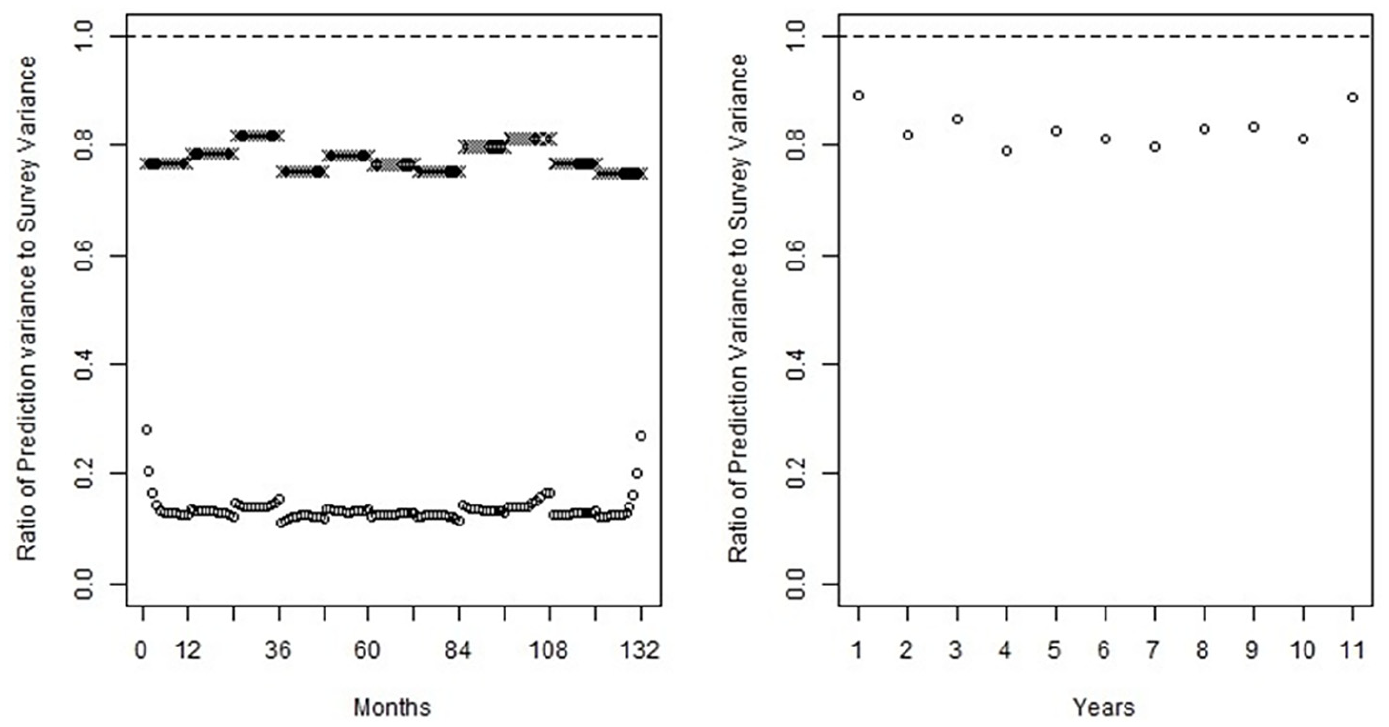
Plot of the ratio of model monthly prediction variances to ACS monthly generated sampling variances in circles, and the ratio of fraction of variance decrease that would be expected from a FH model in hashes (left), and the ratio of model yearly prediction variances to ACS yearly sampling variances (right), in the case where a(z) has roots at z = −1/6 and z = −1/12.
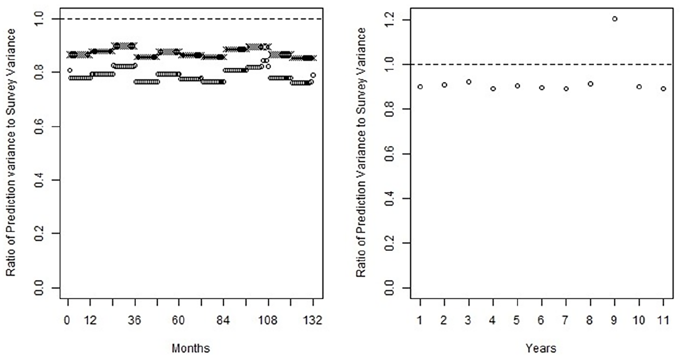
Plot of the ratio of model monthly prediction variances to ACS monthly generated sampling variances in circles, and the ratio of fraction of variance decrease that would be expected from a FH model in hashes (left), and the ratio of model yearly prediction variances to ACS yearly sampling variances (right), in the case where a(z) has roots at z = −4 and z = −2.
Supplement S-3 contains the remaining figures, as well as plots relating the estimator and confidence interval for the estimator with the synthetic sampling distribution data expressed as a 90% confidence interval for each scenario. Subsection S-3.3 provides the inputs from the ACS API, as well as the synthetic data that was generated.
6. Conclusions
This paper studies the problem of customizing flow estimates for survey data, and applies change of support ideas to a time series context, utilizing a continuous-time model for the underlying population process. In particular, we propose using the CARMA class of processes since these have established properties (known formulas for autocovariances, etc.), and outline the general methodology for their application. We focus more specifically on the CAR(1) and CAR(2) processes, noting that some open problems remain on effectively parameterizing higher order CARMA models; the proposed CARMA models can account for some of the temporal dependence in the population process, and the CAR(2) can even accommodate cyclic behavior. Even these fairly simplistic models provide some improvement—based on simulation studies—over more restrictive models, such as that of MPS or FH. Specifically, continuous-time processes appear to have some efficacy for modeling datasets for which a stationarity assumption is tenable; their use appears to outperform the simpler Brownian Motion model, except for cases with more slowly decaying autocovariances, when model and survey error are comparably large.
A remaining research challenge lies in the difficulty of estimating CARMA model parameters. Although the Gaussian likelihood surface is non-convex (such as is commonly the case in discrete time series modeling), the main difficulty is in the parameterization of the space of stable characteristic polynomials. Although it is possible to parameterize the stable polynomials for CAR(1) and CAR(2) processes (the latter case being one of the novel contributions of this paper), for higher order models such a parameterization remains elusive. Given that the present investigation implies that there is utility in using CARMA models for change of support problems, it would be useful to study alternative parameterizations, or perhaps an alternative class of continuous-time models that are more easily parameterized. We remark that the presence of survey error compounds the estimation task.
As for the utility of stock-estimation versus flow-estimation on data simulated from a survey error flow CARMA process, it appears neither method is universally superior in terms of MSE over small domains; however, in terms of the integrated MSE of the prediction function, the flow-based estimation method tends to perform better—since it appears to suffer less from extrapolation challenges at the epoch boundaries. However, when sampling error and model error are comparably large, the stock model appears to have a better MSE for many (but not all) such cases. As a result, this study cannot establish that flow-estimation is better than stock-estimation on flow-observed data drawn from the CARMA class of processes.
This investigation suggests several avenues for further research. First, how to broaden the class of continuous-time models; for CARMA to be implemented, stable parameterization of the higher order models is necessary. Alternatively, other types of models (e.g., marked point processes) for flow-observed data could be proposed instead. Second, alternative methods for fitting (such as a method-of-moments or Bayesian approaches) should be studied, along with corresponding techniques for model selection and fitting. Third, parameter estimation uncertainty should be incorporated into the variance formulas for the custom epoch estimates, and this could be pursued through either a Bayesian apparatus or a parametric bootstrap. We leave these matters for future work.
Supplemental Material
sj-docx-1-jof-10.1177_0282423X241286236 – Supplemental material for Modeling Survey Time Series Data with Flow-Observed CARMA Processes
Supplemental material, sj-docx-1-jof-10.1177_0282423X241286236 for Modeling Survey Time Series Data with Flow-Observed CARMA Processes by Patrick M. Joyce and Tucker S. McElroy in Journal of Official Statistics
Footnotes
Funding
The author(s) received no financial support for the research, authorship, and/or publication of this article.
Disclaimer
This report is released to inform interested parties of research and to encourage discussion. The views expressed on statistical issues are those of the authors and not those of the U.S. Census Bureau.
Supplemental Material
Supplemental material for this article is available online.
Received: September 2023
Accepted: August 2024
References
Supplementary Material
Please find the following supplemental material available below.
For Open Access articles published under a Creative Commons License, all supplemental material carries the same license as the article it is associated with.
For non-Open Access articles published, all supplemental material carries a non-exclusive license, and permission requests for re-use of supplemental material or any part of supplemental material shall be sent directly to the copyright owner as specified in the copyright notice associated with the article.