
Abstract
Small area estimation models are critical for dissemination and understanding of important population characteristics within sub-domains that often have limited sample size. The classic Fay-Herriot model is perhaps the most widely used approach to generate such estimates. However, a limiting assumption of this approach is that the latent true population quantity has a linear relationship with the given covariates. Through the use of random weight neural networks, we develop a Bayesian hierarchical extension of this framework that allows for estimation of nonlinear relationships between the true population quantity and the covariates. We illustrate our approach through an empirical simulation study as well as an analysis of median household income for census tracts in the state of California.
1. Introduction
Large surveys conducted by federal agencies provide a rich set of information about the underlying population from which the sample was taken. Classical design-based estimation methods are often used for population level analysis with such surveys, however, when considering various sub-domains within a population (e.g., county, census tract, etc.), sample sizes are often quite small, leading to unreliable direct estimates.
Small area estimation models overcome the issue of small sample sizes by “borrowing strength” from other sub-domains in the population. For example, the Small Area Income and Poverty Estimates (SAIPE) program and the Small Area Health Insurance Estimates (SAIHE) program are two important use cases for small area estimation models (Bauder et al. 2018; Bell et al. 2016). These models can be conducted either at the area level, or the unit level, however, unit-level models require access to individual microdata which may be confidential (see Parker et al. (2023a, 2023b) for an overview of unit-level modeling approaches). In contrast to this, area-level models are typically feasible for any analyst, as they only require access to the design-based direct estimates, along with their associated uncertainty. These estimates are often disseminated to the public by various federal statistical agencies. Due to small sample sizes, these direct estimates often have substantial uncertainty, and area-level models reduce the uncertainty by smoothing in some fashion, typically through the use of covariates and/or dependence structure.
The popular Fay-Herriot model (Fay and Herriot 1979) is perhaps the most widely used method for constructing small area estimates. The model assumes that the observed direct estimates are equal to the true but unknown population quantity plus a sample-induced noise term. The true quantity is further modeled as a linear combination of some area-level covariates as well as an independent and identically distributed area-level random effect.
There have been numerous extensions to the Fay-Herriot model that relax the various assumptions. These range from spatial and/or temporal dependence among the random effects (Chandra et al. 2015; Chung and Datta 2020; Marhuenda et al. 2013), to modeling of the sample-induced noise term (Parker et al. 2023; Sugasawa et al. 2017; You and Chapman 2006), to incorporating multivariate structure (Porter et al. 2015), among others. One area that has not seen much attention in the literature is relaxation of the linearity assumption, although Giusti et al. (2012) do consider a semi-parametric approach through the use of penalized splines.
In this work we relax the linearity assumption within the Fay-Herriot model, in order to consider general nonlinear relationships between the population quantities of interest and the covariates. Specifically, we model the unknown population quantity as a nonlinear function of input covariates as well as an area-level random effect. The nonlinear function is estimated using a feed-forward neural network where the hidden layer weights are randomly generated and fixed before model fitting. This allows for flexible estimation of the nonlinear mean function at very little computational cost. Importantly, we show that the nonlinear model has the potential for superior prediction and uncertainty quantification compared to the linear alternative. Beyond neural networks, there are a number of popular nonlinear regression techniques, including random forests (Breiman 2001) and gradient boosting (Friedman 2001), among others. However, it is not immediately clear how to embed these approaches into a hierarchical model, such as the Fay-Herriot model, with appropriate uncertainty quantification. Alternatively, Gaussian Process regression is a powerful nonparametric regression tool (Rasmussen and Williams 2006) that naturally fits into a hierarchical framework. Yet, these approaches do not scale well as the number of observations becomes large. In addition, specification of a valid and efficient covariance function can become difficult as the number of covariates grows. Our use of a random weight neural network both fits nicely into the Fay-Herriot model, and scales easily with the number of data points, as demonstrated in the analysis presented in Section 4.
The remainder of this work is outlined as follows. In Section 2 we provide necessary background information and introduce our proposed methodology. Section 3 provides an empirical simulation study using data from the American Community Survey (ACS). In Section 4 we utilize our proposed approach to generate tract level estimates of median household income for the state of California. Finally, we provide discussion and concluding remarks in Section 5.
2. Methodology
Before introducing methodology for small area estimation, we briefly establish some notation. We let
2.1. Basic Fay-Herriot Model
The standard Fay-Herriot model (Fay and Herriot 1979) is written hierarchically as
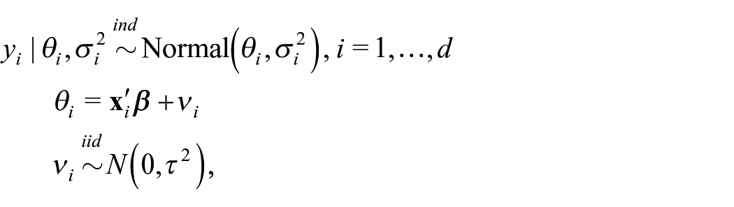
where
2.2. Feed-Forward Neural Networks
Our goal is to replace the linear function assumed by the Fay-Herriot model with a nonlinear function. In other words, rather than assuming
A single layer feed-forward neural network can be written as
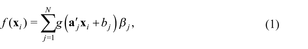
where
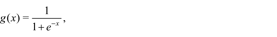
or the ReLU function,

Finally, the parameters
Ordinarily to fit such a model, a loss function would be chosen relating the input data to the response data, and stochastic gradient descent would be used to estimate the entire set of weights (parameters),
The random weight feed-forward neural network may be considered part of the broader class of reservoir computing, where weights are randomly generated rather than estimated. For example, random projection techniques are often used for dimension reduction (Bingham and Mannila 2001) and echo state networks are popular in the context of sequential data (Prokhorov 2005). Still, these random weight methodologies are most often used outside of a statistical context through optimization of a loss function rather than through the use of a likelihood. However, recently the echo state network has been incorporated into a statistical framework under both classical (McDermott and Wikle 2017) and Bayesian (McDermott and Wikle 2019) approaches. Furthermore (Parker and Holan 2023) utilize the random weight feed-forward neural network for unit-level modeling of survey data under informative sampling.
2.3. Nonlinear Fay-Herriot Model
Through the use of a random weight feed-forward neural network, we construct a nonlinear Fay-Herriot model (NFH). We construct the NFH as a Bayesian hierarchical model, allowing for uncertainty quantification as well as regularization of the output layer weights. More specifically, the NFH is written as
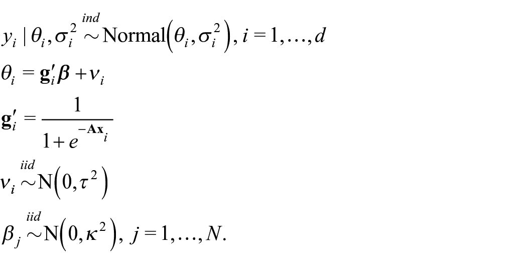
The NFH model requires specification of prior distributions for
The model is completed by placing a prior distribution over the parameters
The Bayesian hierarchical model that makes up the NFH is conditionally conjugate. This allows for the posterior distribution of the NFH model to efficiently be sampled using Gibbs sampling. That is, one can iteratively sample from the following full-conditional distributions:
1.
Here,
2.
3.
Here,
4.
One of the primary advantages of the random weight neural network here is the ability to link the neural network to a likelihood. This is straightforward due to the fact that the hidden layer is completely predetermined before model fitting is done. Thus, linking the neural network to the likelihood is akin to inclusion of extra predictors in the model, where the predictors are the randomly generated outputs of the hidden layer. Furthermore, conditional on the known hidden layer, the model is linear, allowing for a straightforward procedure to sample from the posterior distribution, similar to the linear Fay-Herriot model. Thus, one attains the benefit of a complex nonlinear model with little to no additional computational constraint.
Finally, unlike most machine learning approaches, the random weight neural network used here requires little tuning. Because the hidden layer weights are randomly generated, they do not require tuning parameters related to regularization. We do encourage regularization on the output layer weights, however in our case, this is done naturally through the Bayesian model fitting procedure, again without tuning. Lastly, because we do not use stochastic gradient descent, which is typically required for neural networks, we avoid the need to tune parameters related to optimization. The primary tuning choice to be made with the NFH model is the number of hidden nodes,
3. Empirical Simulation Study
In order to evaluate the utility of the NFH, we construct a simulation study. Rather than simulating data from a parametric model, which could unnecessarily favor one approach, we build our simulation around an existing dataset. Specifically, we obtain the five-year period estimates of median household income at the census tract level for the state of California and treat these estimates as the true population quantity of interest. Doing so preserves existing structure in the underlying data and potential covariates of interest. From there, we generate noise around the “true” values according to the reported sampling errors associated with the original estimates. This results in simulated data with similar structure and sampling error variance as the original dataset. The simulated noisy data can be considered as direct estimates that may be used in a Fay-Herriot or NFH model, and the sampling error variances are still known. Note that the California census tracts result in the number of areas
The primary consideration when fitting the NFH is the choice of how many hidden nodes to include. In order to assess the impact of this choice, we fit variations of the NFH considering
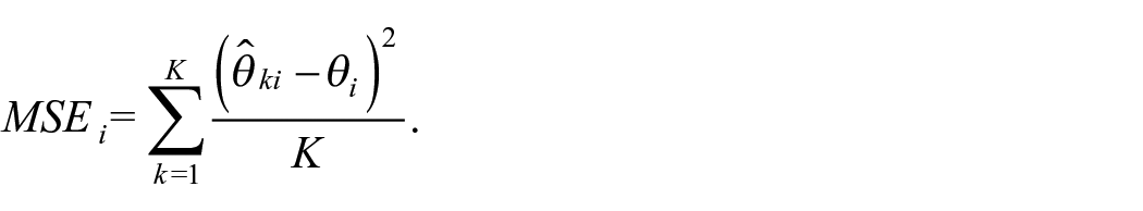
Here,
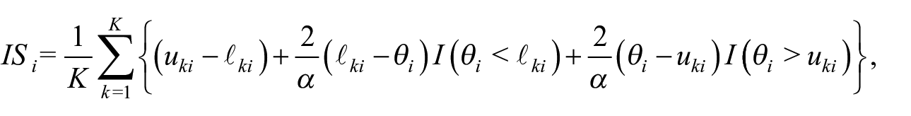
where
Mean Squared Error (MSE), Absolute Bias, Coverage Rate, and Interval Score for the Empirical Simulation Using Tract Level Data from the American Community Survey Five-Year Period Estimates. MSE is Presented Relative to the Direct Estimator. The 25th and 75th Percentiles Are Also Given in Parentheses
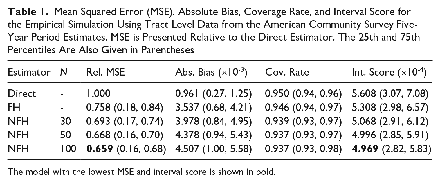
The model with the lowest MSE and interval score is shown in bold.
The direct estimator exhibits roughly zero bias and perfect coverage by design. However, the bias was more or less negligible in all cases given the scale of the data (median household incomes are in the tens of thousands). Interestingly, there is a slight increase in bias as the number of hidden nodes increases for the NFH model. This was investigated by looking at the bias of the fixed effects component only (i.e., not including the random effects) and the opposite pattern was found. In other words, the bias of the fixed effects only component decreases as the number of hidden nodes increases. This leads us to believe that the slight increase in overall bias is due to a slight departure from normality for the random effects as the fixed effects component becomes more complex. If one were strictly interested in decreasing the bias, it might be worth considering more complex models for the random effects. However, in our case, the goal is to reduce the MSE of the point estimates, which is achieved, so we do not pursue more complex random effects models. Unsurprisingly, all model-based approaches outperformed the direct estimator both in terms of MSE as well as interval score. The primary goal of small area estimation is to reduce the uncertainty around the direct estimates, so this result is to be expected. Beyond that, the NFH was able to outperform the standard Fay-Herriot model in all three cases. This indicates that relaxation of the linearity assumption is leading to superior point and uncertainty estimates. As expected, the NFH performs better when a larger number of hidden nodes is selected, although this appears to have diminishing returns, as the gains are minimal between fifty and one hundred nodes. This provides indication that there would be little value to increasing the number of nodes beyond one hundred for this example. Finally, although the NFH has slightly worse interval coverage rate compared to the FH, it results in substantially narrower intervals, leading to an overall preferable interval estimate in terms of the interval score.
Figure 1 examines the MSE for individual tracts, comparing the NFH to FH estimates. Note that the left subplot zooms into a smaller region that contains the majority of the data points for clarity (there are roughly 9,000 total points). The line indicates one-to-one correspondence in MSE, and points falling below the line indicate a reduction in MSE through the use of the NFH when compared to the standard FH. We can see that the majority of points fall below the line, and thus experience reduced MSE through the use of the proposed model. For reference, roughly four out of five tracts exhibited lower MSE from the NFH than the FH. Thus, although the proposed approach did not outperform the FH uniformly, the vast majority of tracts saw an improvement, and there was a substantial improvement on average.
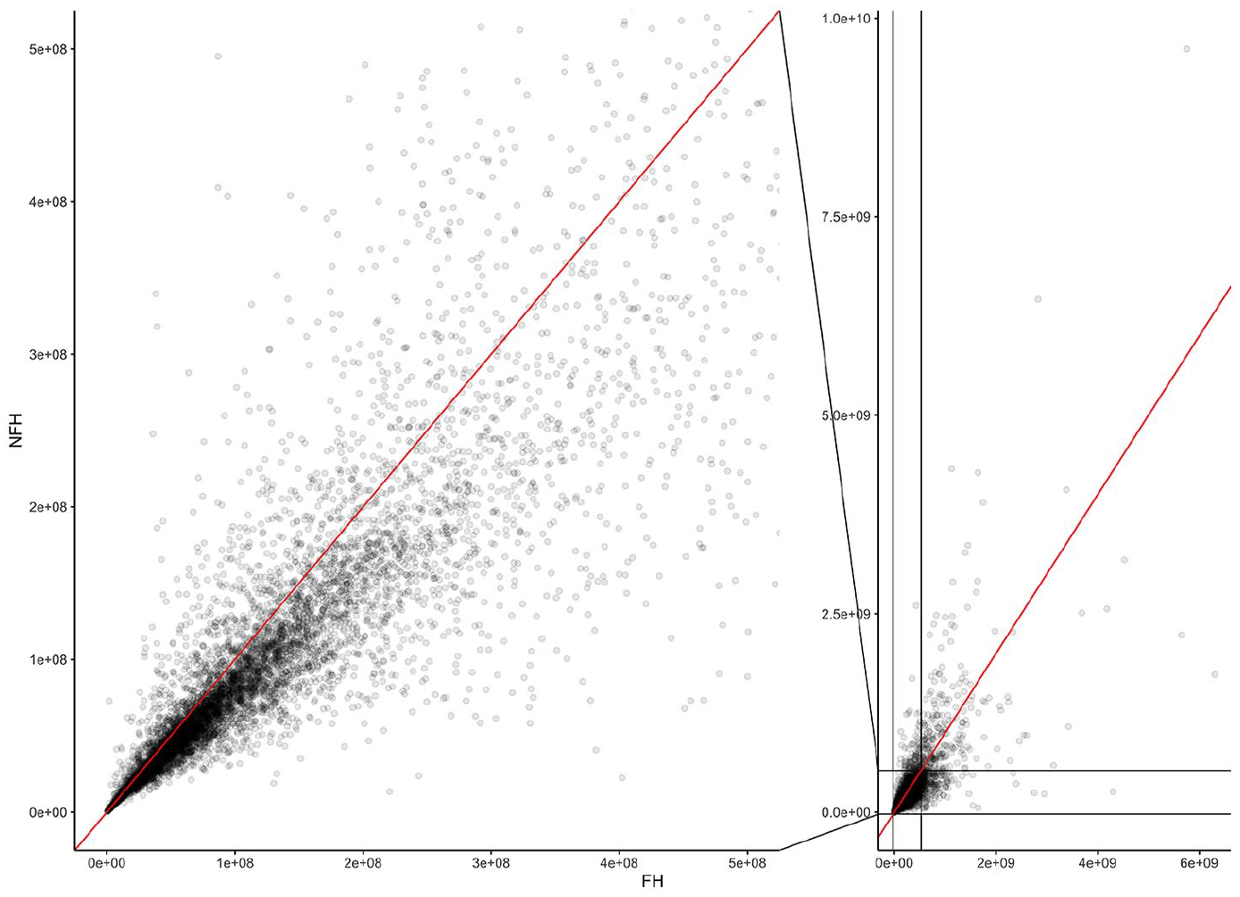
Scatterplot of tract-level MSE of the NFH model versus the FH model for the empirical simulation using tract level data from the American Community Survey five-year period estimates. The left subplot zooms into the region with most of the points.
4. California Median Household Income Estimation
Estimation of household income for various geographic areas is an important use case for small area estimation. For example, both poverty and income county level estimates are produced by the Small Area Income and Poverty Estimates program (SAIPE) (Bell et al. 2016). In fact, these estimates are utilized for administration of various federal programs as well as for local allocation of federal funds (https://www.census.gov/programs-surveys/saipe/about.html).
Using the NFH, we construct estimates of median household income by census tract for the state of California. We use the direct estimates of median household income for the 2021 five-year period based on the American Community Survey as our response, as well as the same covariates outlined in Section 3. California contains 9,129 census tracts, although only 8,927 of these have direct estimates available. Tracts without direct estimates could be due to privacy concerns in the case of extremely small sample size, or due to unpopulated areas, such as industrial land. The direct estimates range from USD8,667 to USD249,901 with a mean of USD90,177 and the sampling standard errors range from about USD63 to USD83,000 with a mean of about USD12,000. Figure 2 shows an exploratory plot of the California median income data. Specifically, we show scatterplots of log median income direct estimates against four different covariates. This exploratory analysis gives early indication that some degree of nonlinearity exists in the relationship between log median income and the covariates. Note that the plots presented only show pairwise relationships between the response of interest and a single covariate, however interactions may exist between the covariates that add another degree of nonlinearity.
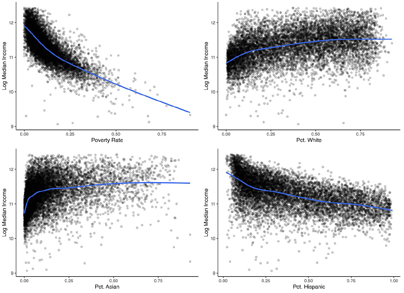
Pairwise scatterplots of log median income versus four covariates for the census tracts in the state of California.
We fit the standard FH model as well as the NFH model using
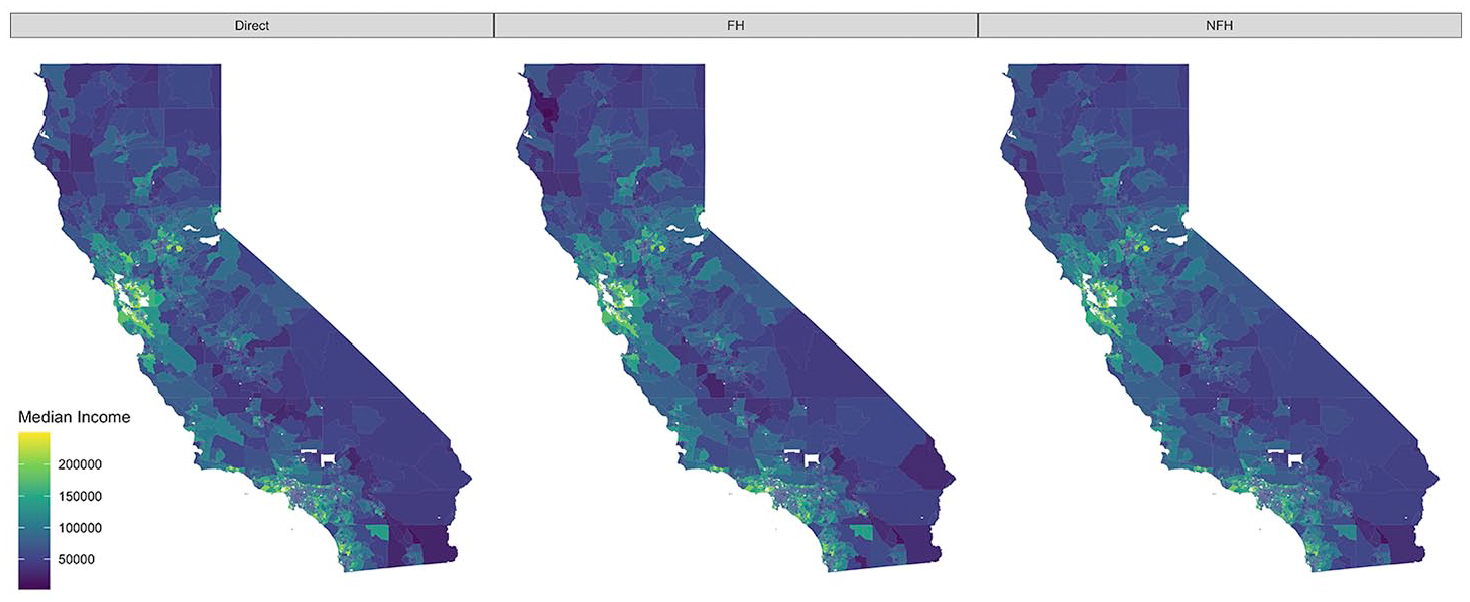
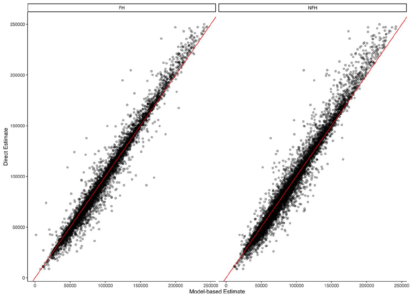
Point estimates of household median income for California census tracts using 2021 American Community Survey five-year period data. Results include direct estimates, Fay-Herriot (FH) estimates, and nonlinear Fay-Herriot (NFH) estimates.
Scatterplots of direct estimates of household median income for California census tracts using 2021 American Community Survey five-year period data versus Fay-Herriot (FH) estimates, and nonlinear Fay-Herriot (NFH) estimates.
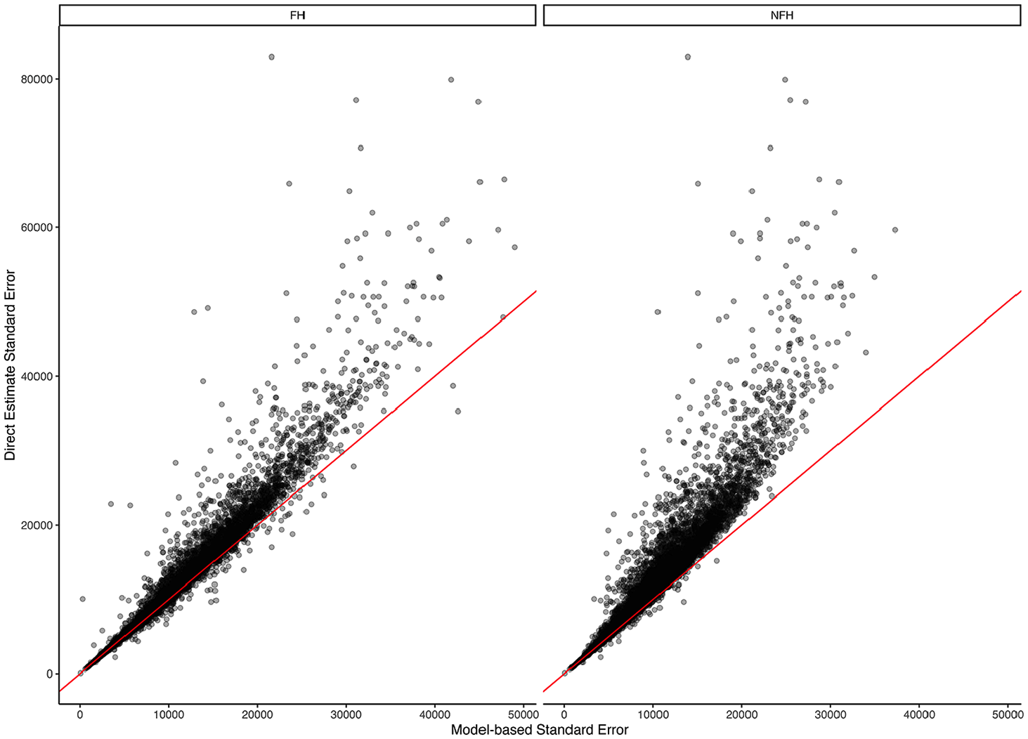
Similarly, Figure 5 shows the standard errors for each of the three estimators. As expected, the largest standard errors are associated with the direct estimators, especially in less populated tracts. Both model-based estimators are able to reduce the standard errors substantially in many cases, however the NFH results in the most reduction, yielding lower standard errors than that of the FH. Finally, Figure 6 shows scatterplots of the direct estimate standard errors versus the two model-based standard errors. Note that points falling above the diagonal line corresponse to a reduction in standard error through the model. As expected, most tracts saw a reduction in standard error when using a model-based approach. This is the primary advantage of SAE models. However, the NFH model results in a greater number of tracts that experience a reduction, and generally larger reductions when compared to the standard FH model.
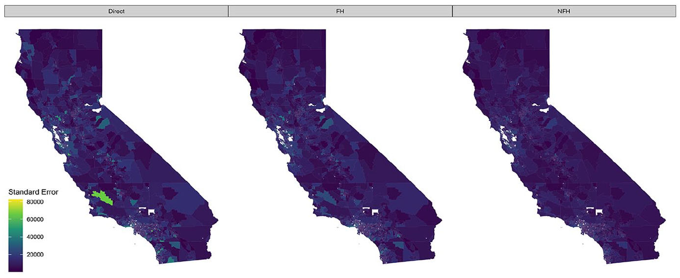
Standard errors of household median income for California census tracts using 2021 American Community Survey five-year period data. Results include direct estimates, Fay-Herriot (FH) estimates, and nonlinear Fay-Herriot (NFH) estimates.
Scatterplots of direct estimate standard errors of household median income for California census tracts using 2021 American Community Survey five-year period data versus Fay-Herriot (FH) standard errors, and nonlinear Fay-Herriot (NFH) standard errors.
One interesting point concerns the variance of the random effects,
Both models were run using a standard 2.3 GHz 8-Core Intel Core i9 processor. The total computation time of the FH was around 17.5 seconds while the total computation time of the NFH was around 76.5 seconds. Thus, although the NFH model took longer in terms of total clock time, both models were extremely quick to run and pose minimal computational burden to the analyst. For reference, the total computation time for the NFH model when using only thirty hidden nodes was roughly thirty-two seconds. Thus, in extremely high-dimensional cases where computation could become a bottle-neck, one may consider using fewer hidden nodes in order to attain computation time on the order of the standard FH model, while still seeing potential gains in precision attributable to the nonlinear model. In total, there is a large potential advantage to the use of the NFH in terms of constructing precise and accurate small area estimates, with little to no trade-off in terms of computational resources that are required.
5. Discussion
Small area estimation is an important problem that offers tremendous value to federal statistical agencies. Area-level models in particular have become widely used, with a great deal of research taking place on how to incorporate various dependence structures into the model. However, the research on nonlinear modeling of covariates for these area-level models has been quite limited. We contribute to the literature by building a nonlinear Fay-Herriot model. Our approach uses random weight neural networks to flexibly model the mean function. A key point is that due to the nature of the hidden layer weights being random, estimation only takes place for the output layer weights, which is straightforward and computationally efficient.
We assess our proposed approach through an empirical simulation study that builds on data from the American Community Survey. We were able to show that the use of the nonlinear Fay-Herriot model has the potential to generate estimates with substantially lower MSE as well as more desirable interval estimates with reduced uncertainty. Finally, we use the NFH model to generate estimates of median household income at the census tract level for the state of California. The R code used to run both the simulation study and the data analysis can be found at https://github.com/paparker/NFH. Importantly, the estimates generated by the NFH approach yielded lower standard errors compared to both the direct estimates as well as the standard linear Fay-Herriot model.
Still, there are some unanswered questions that leave opportunity for future work. First, the NFH proposed herein did not explore spatial or other dependence structure among the random effects. In some cases, different spatial patterns have been observed for different subgroups within the population (Janicki et al. 2022). For such situations, an extension of the NFH that considers nonlinear spatial dependence with covariate interactions could be valuable. One challenge when considering spatial dependence will be the scalability as the number of areas in the model becomes large. Another aspect worth considering is measurement error within the covariates. For example, when covariates are themselves estimated from a survey, there is opportunity to improve the model through acknowledgment of the measurement error process. Although these topics are beyond the scope of the current work, they present interesting future directions.
Finally, the results presented here were based on a relatively small number of covariates. In situations where the number of covariates is large, the number of of potential interactions grows quickly. We suspect that in such situations the linearity assumption becomes quite limiting, and thus we may expect even greater accuracy and precision gains through the use of the proposed nonlinear model.
Footnotes
Acknowledgements
We thank the associate editor and anonymous referees for valuable comments that have helped improve this paper.
Funding
The author disclosed receipt of the following financial support for the research, authorship, and/or publication of this article: This research was partially supported by the U.S. National Science Foundation (NSF) under NSF Grant NCSE-2215169. This article is released to inform interested parties of ongoing research and to encourage discussion. The views expressed on statistical issues are those of the author and not those of the NSF.
Received: September 2023
Accepted: March 2024