Sage Journals: Discover world-class research

Abstract

In this article we consider the price and quantity indices introduced in the nineties by the Italian statistician Marco Martini (1944–2002). It turns out that Fisher indices can be considered as members of the infinite set of Martini indices. In particular attention is paid to the question to what extent these indices exhibit Consistency-in-Aggregation. This throws new light on the behavior of Fisher indices.

Keywords

price index quantity index Martini Fisher Consistency-in-Aggregation

1. Introduction

The first purpose of this theoretical article is to introduce the price and quantity indices named after Marco Martini (1944–2002), an Italian statistician working as full professor at the Università degli Studi di Milano and later at the Università degli Studi di Milano-Bicocca. Biographical details are provided in Martini (2003). His main work in index number theory is contained in the book “I Numeri Indice in un Approccio Assiomatico” (Martini 1992a), of which an English summary appeared in the Journal of the Italian Statistical Society (continued as Statistical Methods & Applications; Martini 1992b). Martini was also a teacher in the former Eurostat-sponsored institute Training of European Statisticians. An Italian version of his lecture notes appeared, the second edition posthumously, under the title “Numeri Indice per il Confronto nel Tempo e nello Spazio” (Martini 2001–2003).

In the course of his work on axiomatic index number theory, Martini defined an infinite set of price and quantity indices with nice properties. It turns out that these indices provide excellent material for illuminating the difference between several concepts of Consistency-in-Aggregation (CIA). This constitutes the second purpose of this article.

The article unfolds as follows. Section 2 discusses definitions and main properties of the Martini indices. Specific among these indices is the pair satisfying the Factor Reversal Test. This pair is shown to be identical to the Fisher indices. Section 3 discusses the various types of CIA proposed in the literature and shows which type is satisfied by the Martini indices. Section 4 discusses two complications with two-stage Martini indices. Section 5 concludes.

2. Definitions

The set of Martini price and quantity indices is a subset of the set of geo-logarithmic price and quantity indices, as introduced by Martini (1992a, 1992b). Though the path followed by Martini in the development of these indices was a bit different, for the definition of Martini indices it is convenient to start with the more familiar Sato-Vartia (SV) indices. The notation continues that of Balk (2008); that is, we consider an aggregate consisting of $N$ commodities over two time periods, with prices $p_{n}^{t}$ and quantities $x_{n}^{t} (n = 1, . . ., N; t = 0, 1)$ ; $p^{t}$ and $x^{t}$ denote vectors of prices and quantities, respectively; and a dot denotes their inner product. Prices and quantities are assumed to be positive.

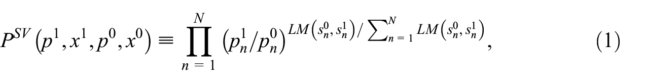
The Sato-Vartia (SV) indices are geometric means of price or quantity relatives. These relatives are weighed with logarithmic mean value shares, normalized to ensure that these add up to 1. Thus, the Sato-Vartia price index is defined as

P^{SV} (p^{1}, x^{1}, p^{0}, x^{0}) \equiv Π_{n = 1}^{N} {(p_{n}^{1} / p_{n}^{0})}^{LM (s_{n}^{0}, s_{n}^{1}) / \sum_{n = 1}^{N} LM (s_{n}^{0}, s_{n}^{1})},

(1)

where $LM (.)$ denotes the logarithmic mean and elementary value shares are defined as $s_{n}^{t} \equiv p_{n}^{t} x_{n}^{t} / p^{t} \cdot x^{t} (n = 1, . . ., N; t = 0, 1)$ . The Sato-Vartia quantity index is defined as $Q^{SV} (p^{1}, x^{1}, p^{0}, x^{0}) \equiv P^{SV} (x^{1}, p^{1}, x^{0}, p^{0})$ ; that is, price and quantity indices have the same mathematical form whereby prices and quantities are interchanged. It is straightforward to check that $P^{SV} (p^{1}, x^{1}, p^{0}, x^{0}) \times Q^{SV} (p^{1}, x^{1}, p^{0}, x^{0}) = p^{1} \cdot x^{1} / p^{0} \cdot x^{0}$ ; that is, the SV indices satisfy the Factor Reversal Test. Further properties of the SV indices are discussed in Balk (2008, 85–6). Recall that for any two positive real numbers $a$ and $b$ their logarithmic mean is defined by $LM (a, b) \equiv (a - b) / \ln (a / b)$ when $a \neq b$ , and $LM (a, a) \equiv a$ . By the logarithmic mean any difference can be transformed into a ratio and vice versa. The logarithmic mean has all the properties of a mean, and lies between the geometric mean and the arithmetic mean. See Balk (2008, 134–6) for details.

Consider now the SV price index. Replace the comparison period quantity vector $x^{1}$ by the vector ${(x^{1})}^{α} ☆ {(x^{0})}^{1 - α}$ and the base period quantity vector $x^{0}$ by the vector ${(x^{1})}^{β} ☆ {(x^{0})}^{1 - β}$ , where ${(x^{t})}^{ℓ}$ denotes the vector of ${(x_{n}^{t})}^{ℓ} (n = 1, . . ., N; t = 0, 1; ℓ = α, 1 - α, β, 1 - β)$ , $☆ denotes$ the elementwise vector product, and the real numbers $α, β \in [0, 1]$ . Thus each element of $x^{t} (t = 0, 1)$ is replaced by a convex combination of period 0 and period 1 quantities. Then $P^{SV} (p^{1}, {(x^{1})}^{α} ☆ {(x^{0})}^{1 - α}, p^{0}, {(x^{1})}^{β} ☆ {(x^{0})}^{1 - β})$ as function of $p^{1}, x^{1}, p^{0}, x^{0}$ defines a geo-logarithmic price index. The axiomatic properties of the infinite set of geo-logarithmic price indices were studied by Fattore (2010a, 2010b). Notice that choosing $α = 1$ and $β = 0$ leads back to the SV index. 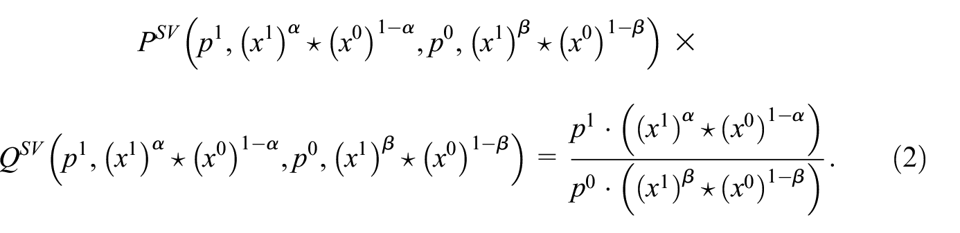For completeness’ sake it is mentioned that Białek (2019) considered the larger set of indices defined as $[P^{SV} (p^{1}, {(x^{1})}^{α} ☆ {(x^{0})}^{1 - α}, p^{0}, {(x^{1})}^{β} ☆ {(x^{0})}^{1 - β} {)]}^{γ} [P^{SV} (p^{1}, {(x^{1})}^{1 - α} ☆ {(x^{0})}^{α}, p^{0}, {(x^{1})}^{1 - β} ☆ {(x^{0})}^{β} {)]}^{1 - γ}$ with $γ \in [0, 1]$ .

As the SV indices satisfy the Factor Reversal Test, the following relation holds:

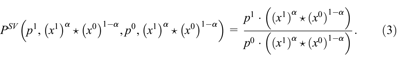
\begin{matrix} P^{SV} (p^{1}, {(x^{1})}^{α} ☆ {(x^{0})}^{1 - α}, p^{0}, {(x^{1})}^{β} ☆ {(x^{0})}^{1 - β}) \times \\ Q^{SV} (p^{1}, {(x^{1})}^{α} ☆ {(x^{0})}^{1 - α}, p^{0}, {(x^{1})}^{β} ☆ {(x^{0})}^{1 - β}) = \frac{p^{1} \cdot ({(x^{1})}^{α} ☆ {(x^{0})}^{1 - α})}{p^{0} \cdot ({(x^{1})}^{β} ☆ {(x^{0})}^{1 - β})} . \end{matrix}

(2)

Let $α = β$ . As the SV quantity index satisfies the Identity Axiom, Equation (2) reduces to

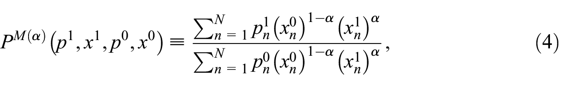
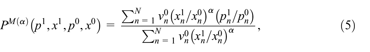
P^{SV} (p^{1}, {(x^{1})}^{α} ☆ {(x^{0})}^{1 - α}, p^{0}, {(x^{1})}^{α} ☆ {(x^{0})}^{1 - α}) = \frac{p^{1} \cdot ({(x^{1})}^{α} ☆ {(x^{0})}^{1 - α})}{p^{0} \cdot ({(x^{1})}^{α} ☆ {(x^{0})}^{1 - α})} .

(3)

The right-hand side of Equation (3) defines the infinite set of Martini price indices. Using more conventional notation, the definition of the Martini (1992a, 1992b) price indices reads

P^{M (α)} (p^{1}, x^{1}, p^{0}, x^{0}) \equiv \frac{\sum_{n = 1}^{N} p_{n}^{1} {(x_{n}^{0})}^{1 - α} {(x_{n}^{1})}^{α}}{\sum_{n = 1}^{N} p_{n}^{0} {(x_{n}^{0})}^{1 - α} {(x_{n}^{1})}^{α}},

(4)

for real numbers $α \in [0, 1]$ . Notice that any Martini price index can be considered as a Lowe price index, comparing prices of period 1 to those of period 0 by weighing them with quantities that are convex combinations of period 0 and period 1 quantities. Recall that the generic formula of a Lowe price index is $p^{1} \cdot x / p^{0} \cdot x$ , where $x$ is some vector of quantities.

An alternative way of writing Equation (4) is as weighted arithmetic mean of price relatives,

P^{M (α)} (p^{1}, x^{1}, p^{0}, x^{0}) = \frac{\sum_{n = 1}^{N} v_{n}^{0} {(x_{n}^{1} / x_{n}^{0})}^{α} (p_{n}^{1} / p_{n}^{0})}{\sum_{n = 1}^{N} v_{n}^{0} {(x_{n}^{1} / x_{n}^{0})}^{α}},

(5)

where elementary values are defined as $v_{n}^{t} \equiv p_{n}^{t} x_{n}^{t} (n = 1, . . ., N; t = 0, 1)$ . The weights of the price relatives are elementary values of the base period 0 which are updated by quantity relatives to the power $α$ . The Martini price index with $α = 0$ reduces to the Laspeyres price index, with $α = 1$ to the Paasche price index, and with $α = 1 / 2$ to the Walsh-1 price index.

The Martini quantity indices are defined as $Q^{M (α)} (p^{1}, x^{1}, p^{0}, x^{0}) \equiv P^{M (α)} (x^{1}, p^{1}, x^{0}, p^{0})$ , for real numbers $α \in [0, 1]$ . These indices compare quantities of period 1 to those of period 0 by weighing them with prices that are convex combinations of period 0 and period 1 prices. They can alternatively be written as weighted arithmetic means of quantity relatives, weights being now elementary values of the base period 0 which are updated with price relatives to the power $α$ . The Martini quantity index with $α = 0$ reduces to the Laspeyres quantity index, with $α = 1$ to the Paasche quantity index, and with $α = 1 / 2$ to the Walsh-1 quantity index.

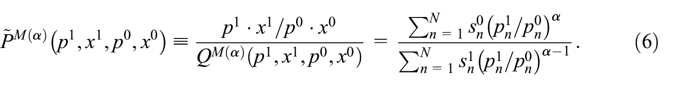
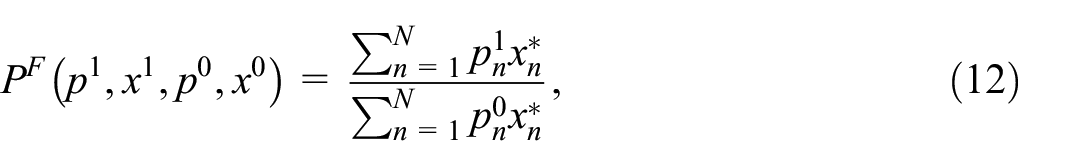
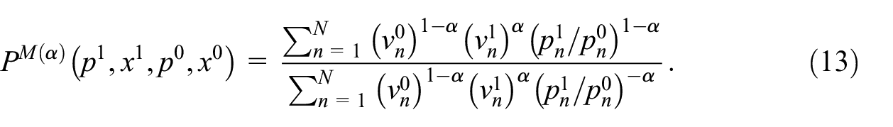
The generic formula of the Martini implicit price index, defined as value ratio divided by quantity index, reads

{\tilde{P}}^{M (α)} (p^{1}, x^{1}, p^{0}, x^{0}) \equiv \frac{p^{1} \cdot x^{1} / p^{0} \cdot x^{0}}{Q^{M (α)} (p^{1}, x^{1}, p^{0}, x^{0})} = \frac{\sum_{n = 1}^{N} s_{n}^{0} {(p_{n}^{1} / p_{n}^{0})}^{α}}{\sum_{n = 1}^{N} s_{n}^{1} {(p_{n}^{1} / p_{n}^{0})}^{α - 1}} .

(6)

The Martini implicit quantity index has the same functional form, with price relatives replaced by quantity relatives.

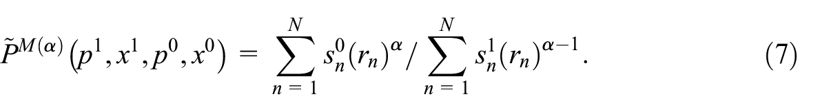
The Martini price and quantity indices, as well as the implicit indices, satisfy the basic axioms concerning Monotonicity, Linear Homogeneity, Identity, Homogeneity of Degree 0, and Dimensional Invariance. Fattore (2010a, Proposition 6; 2010b, Proposition 5) showed that in certain situations the implicit indices may violate monotonicity. Such situations are, however, rather unlikely to occur. Consider, for instance, the implicit price index. Letting $r_{n} \equiv p_{n}^{1} / p_{n}^{0} (n = 1, . . ., N)$ , Equation (6) can be written as

{\tilde{P}}^{M (α)} (p^{1}, x^{1}, p^{0}, x^{0}) = \sum_{n = 1}^{N} s_{n}^{0} {(r_{n})}^{α} / \sum_{n = 1}^{N} s_{n}^{1} {(r_{n})}^{α - 1} .

(7)

It is reassuring to notice that if $s_{n}^{0} = s_{n}^{1} (n = 1, . . ., N)$ then $\partial {\tilde{P}}^{M (α)} (p^{1}, x^{1}, p^{0}, x^{0}) / \partial r_{n} > 0$ if $α \in [0, 1]$ .

The indices do neither satisfy the Circularity (Transitivity) Test, nor the Time Reversal Test (except if $α = 1 / 2$ ). Though $P^{M (α)} (.)$ and $Q^{M (α)} (.)$ have the same functional form, the Factor Reversal Test is in general not satisfied. All these axioms and tests were formally defined and discussed in Balk (2008).

Interestingly, there exists a unique $α^{*}$ such that the Factor Reversal Test is satisfied; that is,

P^{M (α^{*})} (p^{1}, x^{1}, p^{0}, x^{0}) \times Q^{M (α^{*})} (p^{1}, x^{1}, p^{0}, x^{0}) = p^{1} \cdot x^{1} / p^{0} \cdot x^{0} .

(8)

This can be seen as follows. By substituting Equation (6), for general $α$ the Factor Reversal Test can be rewritten as

P^{M (α)} (p^{1}, x^{1}, p^{0}, x^{0}) = {\tilde{P}}^{M (α)} (p^{1}, x^{1}, p^{0}, x^{0}) .

(9)

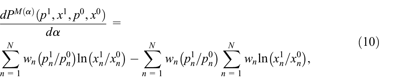
If $α$ goes from 0 to 1 then the left-hand side ascends/descends monotonously from Laspeyres to Paasche whereas the right-hand side descends/ascends monotonously from Paasche to Laspeyres (Martini 1992a, Theorem 4.2.3). The simple proof of the monotonicity in $α$ of the left-hand side runs as follows, restated in our notation. It is straightforward to show that

\begin{matrix} \frac{d P^{M (α)} (p^{1}, x^{1}, p^{0}, x^{0})}{d α} = \\ \sum_{n = 1}^{N} w_{n} (p_{n}^{1} / p_{n}^{0}) \ln (x_{n}^{1} / x_{n}^{0}) - \sum_{n = 1}^{N} w_{n} (p_{n}^{1} / p_{n}^{0}) \sum_{n = 1}^{N} w_{n} \ln (x_{n}^{1} / x_{n}^{0}), \end{matrix}

(10)

where $w_{n} \equiv v_{n}^{0} {(x_{n}^{1} / x_{n}^{0})}^{α} / \sum_{n = 1}^{N} v_{n}^{0} {(x_{n}^{1} / x_{n}^{0})}^{α} (n = 1, . . ., N)$ . This is a weighted covariance of price relatives $p_{n}^{1} / p_{n}^{0}$ and quantity percentage changes $\ln (x_{n}^{1} / x_{n}^{0})$ , the sign of which is independent of the value of $α$ . For the right-hand side of Equation (9) we must consider $d Q^{M (α)} (.) / d α$ , for which a similar covariance results. Thus, there must exist a unique $α^{*}$ for which both sides of Equation (9) are equal.

The pair of indices $(P^{M (α^{*})} (.), Q^{M (α^{*})} (.))$ will be called Martini ideal indices. Notice that, though an explicit form cannot be provided, $α^{*}$ is a function of the data set $(p^{1}, x^{1}, p^{0}, x^{0})$ . Without the bond between parameter $α$ and dataset on which the indices are compiled the Factor Reversal relation is unlikely to hold. Equation (8) implies that $P^{M (α^{*})} (.)$ can be considered as a generalized unit value index; see von Auer (2014) for the definition of such an index.

Quite surprisingly, and unnoticed in the literature, the same argument leads to the conclusion that there exists a unique $α^{* *}$ such that

P^{M (α^{* *})} (p^{1}, x^{1}, p^{0}, x^{0}) = P^{F} (p^{1}, x^{1}, p^{0}, x^{0}),

(11)

where $P^{F} (.)$ denotes the Fisher price index. As the Fisher index is the simple geometric mean of Laspeyres and Paasche indices and, if $α$ goes from 0 to 1 then the Martini index $P^{M (α)} (.)$ moves monotonously from Laspeyres to Paasche or vice versa, there must exist a unique $α^{* *}$ such that Equation (11) holds. Since the Fisher indices satisfy the Factor Reversal Test, the final conclusion must be that $α^{*} = α^{* *}$ ; that is, Martini ideal indices are identical to Fisher indices.

A useful corollary to this conclusion is that the Fisher indices can be expressed as Martini (or Lowe) indices; for example,

P^{F} (p^{1}, x^{1}, p^{0}, x^{0}) = \frac{\sum_{n = 1}^{N} p_{n}^{1} x_{n}^{*}}{\sum_{n = 1}^{N} p_{n}^{0} x_{n}^{*}},

(12)

where $x_{n}^{*} \equiv {(x_{n}^{0})}^{1 - α^{*}} {(x_{n}^{1})}^{α^{*}} (n = 1, . . ., N)$ . As the quantity vector $x^{*}$ depends, via $α^{*}$ , on $p^{0}, x^{0}, p^{1}, x^{1}$ , this result does not contradict Proposition 1 of Yu (2023). We will come back to this result in the concluding section.

3. Consistency-in-Aggregation

To start with, it is useful to realize that any index satisfying invariance to the units of measurement of the elementary commodities (aka the Dimensional Invariance axioms) can be written as a function of elementary price relatives $p_{n}^{1} / p_{n}^{0}$ or quantity relatives $x_{n}^{1} / x_{n}^{0}$ and elementary values $v_{n}^{0}$ and $v_{n}^{1} (n = 1, . . ., N)$ . For example, Equation (5) can be written as

P^{M (α)} (p^{1}, x^{1}, p^{0}, x^{0}) = \frac{\sum_{n = 1}^{N} {(v_{n}^{0})}^{1 - α} {(v_{n}^{1})}^{α} {(p_{n}^{1} / p_{n}^{0})}^{1 - α}}{\sum_{n = 1}^{N} {(v_{n}^{0})}^{1 - α} {(v_{n}^{1})}^{α} {(p_{n}^{1} / p_{n}^{0})}^{- α}} .

(13)

Let us call the aggregate of commodities $1, . . ., N A$ , and let $A$ be partitioned arbitrarily into $K$ subaggregates $A_{k}$ ,

A = \cup_{k = 1}^{K} A_{k}, A_{k} \cap A_{l} = Ø (k \neq l) .

(14)

Each subaggregate consists of a certain number of commodities. Let $N_{k} \geq 1$ denote the number of commodities contained in $A_{k} (k = 1, . . ., K)$ . Obviously $N = \sum_{k = 1}^{K} N_{k}$ . Let $(p_{k}^{1}, x_{k}^{1}, p_{k}^{0}, x_{k}^{0})$ be the subvector of $(p^{1}, x^{1}, p^{0}, x^{0})$ corresponding to the subaggregate $A_{k}$ . Recall that $v_{n}^{t} \equiv p_{n}^{t} x_{n}^{t}$ is the value of commodity $n$ at period $t$ . Then $V_{k}^{t} \equiv \sum_{n \in A_{k}} v_{n}^{t} (k = 1, . . ., K)$ is the value of subaggregate $A_{k}$ at period $t$ , and $V^{t} \equiv \sum_{n \in A} v_{n}^{t} = \sum_{k = 1}^{K} V_{k}^{t}$ is the value of aggregate $A$ at period $t$ .

There is quite some literature on the concept of CIA, summarized by Balk (2008, Subsections 3.7 and 3.10.3) and Von Auer and Wengenroth (2021). The basic requirements are the following two:

(i)the index number for the aggregate $A$ , which is defined as the outcome of a single-stage index, can also be computed in two stages, namely by first computing the index numbers for the subaggregates $A_{k} (k = 1, . . ., K)$ and from these the index number for the aggregate;

(ii)the indices used in the single-stage computation and those used in the first-stage computation have the same functional form (except for the dimension of the variables).

Many indices satisfy these two requirements, as shown in the classification provided by Von Auer and Wengenroth (2021). The next requirement, however, severely limits the number of indices exhibiting CIA:

(iii) the formula used in the second-stage computation has the same functional form (except possibly for the dimension of the variables) as the indices used in the single stage and the index used in the first stage after the following transformation has been applied: commodity price or quantity relatives are replaced by subaggregate indices and commodity values are replaced by subaggregate values.

Balk (2008, 109) formalized the joint requirements (i) to (iii) as tests for price indices and quantity indices. The Appendix contains the details.

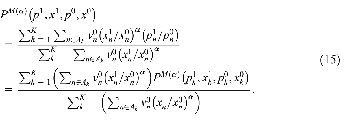
Let us now look at a Martini price index for the aggregate $A$ . With obvious modifications the same story of course holds for a quantity index. By expanding Equation (5) and applying the price index definition at subaggregate level, we obtain

\begin{matrix} P^{M (α)} (p^{1}, x^{1}, p^{0}, x^{0}) \\ = \frac{\sum_{k = 1}^{K} \sum_{n \in A_{k}} v_{n}^{0} {(x_{n}^{1} / x_{n}^{0})}^{α} (p_{n}^{1} / p_{n}^{0})}{\sum_{k = 1}^{K} \sum_{n \in A_{k}} v_{n}^{0} {(x_{n}^{1} / x_{n}^{0})}^{α}} \\ = \frac{\sum_{k = 1}^{K} (\sum_{n \in A_{k}} v_{n}^{0} {(x_{n}^{1} / x_{n}^{0})}^{α}) P^{M (α)} (p_{k}^{1}, x_{k}^{1}, p_{k}^{0}, x_{k}^{0})}{\sum_{k = 1}^{K} (\sum_{n \in A_{k}} v_{n}^{0} {(x_{n}^{1} / x_{n}^{0})}^{α})} . \end{matrix}

(15)

It is immediately clear that the requirements (i) and (ii) are satisfied. Put otherwise, a Martini price index is, using the terminology of Von Auer and Wengenroth (2021), CIA with respect to the secondary attribute $z_{n} \equiv v_{n}^{0} {(x_{n}^{1} / x_{n}^{0})}^{α} (n = 1, . . ., N)$ . Martini (1992a, 35; 2001–2003, 103) would call this associativity. The important characteristic is that the outcome of the formula on the last line of Equation (15) does not depend on the particular partition of the aggregate $A$ that has been chosen.

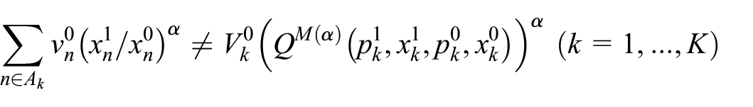
Requirement (iii), however, will in general be violated, because

\sum_{n \in A_{k}} v_{n}^{0} {(x_{n}^{1} / x_{n}^{0})}^{α} \neq V_{k}^{0} {(Q^{M (α)} (p_{k}^{1}, x_{k}^{1}, p_{k}^{0}, x_{k}^{0}))}^{α} (k = 1, . . ., K)

for $α \neq 0, 1$ . Thus, although a Martini price index for the aggregate is a weighted mean of Martini price indices for the subaggregates, it is not a Martini price index of Martini price indices. Put otherwise, the aggregate index number cannot be calculated from the subaggregate index numbers by weighing with functions of subaggregate values $V_{k}^{0}$ and quantity index numbers $Q^{M (α)} (p_{k}^{1}, x_{k}^{1}, p_{k}^{0}, x_{k}^{0})$ . Again in the words of Von Auer and Wengenroth (2021), the relationship $z_{n} = v_{n}^{0} {(x_{n}^{1} / x_{n}^{0})}^{α}$ does not carry over from the commodity level to the (sub-)aggregate level.

This implies a disadvantage in statistical practice. Consider a statistical agency where various departments are engaged in compiling, calculating, or estimating, subaggregate price and quantity index numbers, $P^{M (α)} (p_{k}^{1}, x_{k}^{1}, p_{k}^{0}, x_{k}^{0})$ and $Q^{M (α)} (p_{k}^{1}, x_{k}^{1}, p_{k}^{0}, x_{k}^{0}) (k = 1, . . ., K)$ from elementary commodity data. And let there be some department, for instance the National Accounts department, the task of which it is to put the various pieces together with help of subaggregate value data. Then the overall price index resulting from this process does not coincide with any price index hypothetically computed directly from the elementary data unless this department has access to all the sums of secondary attributes corresponding to the subaggregates, $\sum_{n \in A_{k}} z_{n} (k = 1, . . ., K)$ . For this, however, the elementary commodity values and quantity relatives are still indispensable. Even in the “big data” era it is unthinkable that every department has access to all the millions of microdata underlying, say, GDP. And what to think of academic researchers?

The conclusion is that though a Martini index is CIA (with respect to a certain secondary attribute) in the sense of Von Auer and Wengenroth (2021), it violates the stronger form of CIA. Notice that the index does satisfy the Equality Test, which says that if all the subaggregate index numbers are equal, $P^{M (α)} (p_{k}^{1}, x_{k}^{1}, p_{k}^{0}, x_{k}^{0}) = λ (k = 1, . . ., K)$ , then the index number for the aggregate is also equal to $λ$ .

4. Some Implications for Applied Work

If one wants to employ a Martini price or quantity index in applied work there appear to be at least two complications. The first is that violation of CIA in the sense of (i) to (iii) implies that the overall two-stage price index number depends on the particular partition of the aggregate $A$ that was chosen. This can be seen as follows.

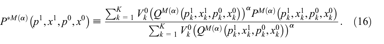
Given all the individual price and quantity data, the single-stage Martini price index for the aggregate $A$ is given by Equation (5). For the partition specified in Equation (14) the two-stage Martini index, that is, the Martini index of Martini indices, is defined as

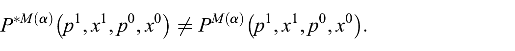
P^{* M (α)} (p^{1}, x^{1}, p^{0}, x^{0}) \equiv \frac{\sum_{k = 1}^{K} V_{k}^{0} {(Q^{M (α)} (p_{k}^{1}, x_{k}^{1}, p_{k}^{0}, x_{k}^{0}))}^{α} P^{M (α)} (p_{k}^{1}, x_{k}^{1}, p_{k}^{0}, x_{k}^{0})}{\sum_{k = 1}^{K} V_{k}^{0} {(Q^{M (α)} (p_{k}^{1}, x_{k}^{1}, p_{k}^{0}, x_{k}^{0}))}^{α}} .

(16)

As a Martini index does not exhibit CIA in the sense of (i) to (iii), this will generally give a different outcome; that is,

P^{* M (α)} (p^{1}, x^{1}, p^{0}, x^{0}) \neq P^{M (α)} (p^{1}, x^{1}, p^{0}, x^{0}) .

It is now important to realize that the outcome of the two-stage index depends on the particular partition of the aggregate $A$ that has been chosen. The effect of this was demonstrated empirically in the article by Zavanella and Pirotta (2021). Though their research was concerned with quantity indices its conclusion applies mutatis mutandis to price indices.

The elementary data used by Zavanella and Pirotta (2021) were quantity index numbers and values of capital and labor input for seventeen industrial sectors in Italy over the period 1995 to 2014. The objective was to compile annual (chained) quantity index numbers for aggregate industrial input. The first partition concerned the seventeen sectors (their Table 2), the second partition concerned the two input categories (their Table 3). Biancamaria Zavanella advised me that the column “Martini aggregated” in Table 2 is incorrect. The other columns, Table 3, and the figures are correct. It is interesting to compare $Q^{M (α)} (.)$ and $Q^{* M (α)} (.)$ for the two different partitions of the overall aggregate. The authors repeated the same exercise with Törnqvist quantity indices, and concluded that the performance (in terms of the difference between the two-stage index numbers of the two partitions) of the Martini indices was better.

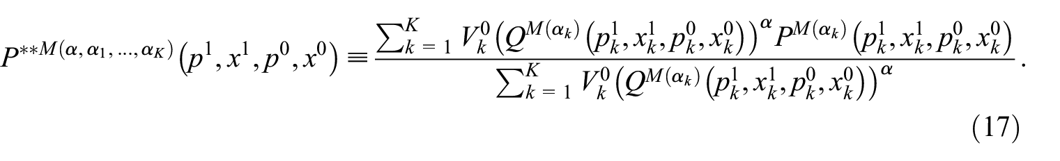
The second complication has to do with the choice of the parameter $α$ . In Zavanella and Pirotta’s exercise the value of $α$ for each pair of adjacent years has been chosen such that $P^{M (α)} (p^{1}, x^{1}, p^{0}, x^{0})$ is ideal. But then the first-stage subaggregate indices $P^{M (α)} (p_{k}^{1}, x_{k}^{1}, p_{k}^{0}, x_{k}^{0})$ , as well as the second-stage index will generally not be ideal.

On the other hand, at subaggregate level one can opt for ideal Martini indices $P^{M (α_{k})} (p_{k}^{1}, x_{k}^{1}, p_{k}^{0}, x_{k}^{0})$ and then compute, for a certain value of the parameter $α$ , as two-stage index

P^{* * M (α, α_{1}, \dots, α_{K})} (p^{1}, x^{1}, p^{0}, x^{0}) \equiv \frac{\sum_{k = 1}^{K} V_{k}^{0} {(Q^{M (α_{k})} (p_{k}^{1}, x_{k}^{1}, p_{k}^{0}, x_{k}^{0}))}^{α} P^{M (α_{k})} (p_{k}^{1}, x_{k}^{1}, p_{k}^{0}, x_{k}^{0})}{\sum_{k = 1}^{K} V_{k}^{0} {(Q^{M (α_{k})} (p_{k}^{1}, x_{k}^{1}, p_{k}^{0}, x_{k}^{0}))}^{α}} .

(17)

But even if $α$ was selected such that also the second-stage index is ideal, the outcomes of $P^{* * M (α, α_{1}, . . ., α_{K})} (.)$ , $P^{* M (α)} (.)$ , and $P^{M (α)} (.)$ will in general be different.

5. Conclusion

Martini indices with $α \neq 0, 1$ have not been employed by statistical agencies. I believe that the only exception is Statistics Sweden in their Consumer Price Index. The article by Zavanella and Pirotta (2021) is, as far as I know, the first application on actual data. The requirement to have data from two periods makes it hard to compile the indices in real time. Two other disadvantages are:

The fact that a particular choice must be made for the parameter $α$ . The three most natural choices (0, 1/2, 1) bring us back to the well-known indices of Laspeyres, Walsh, and Paasche. Choosing $α$ such that the index and its co-factor satisfy the Factor Reversal Test returns the Fisher index.

A Martini index with $α \neq 0, 1$ does not satisfy CIA in the sense of (i) to (iii). Recall that requirement (iii) is important for statistical practice as well as applications. Violation of the strong form of CIA implies that, as illustrated in the previous section, outcomes not only depend on a particular choice of $α$ but also on the compilation strategy. Whether the differences between various outcomes are deemed large or small depends of course on the particular application.

From a theoretical perspective, however, the Martini indices appear to be interesting constructs. It has been shown that Fisher indices can be considered as members of the infinite set of Martini indices. This fact can then be used to throw additional light on the behavior of the widely used Fisher indices with respect to CIA. Though not CIA in the sense of (i) to (iii), the Fisher price index, for instance, is CIA with respect to the single secondary attribute $v_{n}^{0} {(x_{n}^{1} / x_{n}^{0})}^{α^{* *}} (n = 1, . . ., N)$ , where $α^{* *}$ is the solution of Equation (11). Calculation of a two-stage Fisher index then implies that one has to deal with $K$ distinct $α$ ’s for the subaggregates plus one $α$ for combining the subaggregate indices to obtain the aggregate index. The extent to which all these $α$ ’s are different can be considered as a measure for Fisher’s performance with respect to CIA.

Footnotes

Appendix

As addition is the simplest form of aggregation we start by considering the aggregate value difference. Suppose this difference can be decomposed into two parts by means of functions $P (.)$ and $Q (.)$ ,

(A1)

V^{1} - V^{0} = p^{1} \cdot x^{1} - p^{0} \cdot x^{0} = P (p^{1}, x^{1}, p^{0}, x^{0}) + Q (p^{1}, x^{1}, p^{0}, x^{0}) .

The first function, $P (.)$ , is supposed to measure the part of the value difference that is due to differing prices and the second function, $Q (.)$ , the part of the value difference that is due to differing quantities. It is supposed that these two functions, called indicators, satisfy the following basic requirements:

The last axiom has an important consequence. Let $Λ$ be the diagonal matrix with elements $1 / p_{n}^{0} (n = 1, . . ., N)$ . Then

(A2)

P (p^{1}, x^{1}, p^{0}, x^{0}) = P (p^{1} / p^{0}, p^{0} ☆ x^{1}, 1_{N}, v^{0})

in which $p^{1} / p^{0}$ denotes the vector of price relatives $p_{n}^{1} / p_{n}^{0}$ , $p^{0} ☆ x^{1}$ denotes the vector of $p_{n}^{0} x_{n}^{1}$ , $1_{N}$ denotes the vector consisting of $N$ ones, and $v^{0}$ denotes the vector of $v_{n}^{0} \equiv p_{n}^{0} x_{n}^{0} (n = 1, . . ., N)$ . As $p_{n}^{0} x_{n}^{1} = p_{n}^{1} x_{n}^{1} / (p_{n}^{1} / p_{n}^{0}) = v_{n}^{1} / (p_{n}^{1} / p_{n}^{0}) (n = 1, . . ., N)$ it is clear that any $P (.)$ can be written as a function $ψ (.)$ of only $3 N$ variables, namely price relatives $p_{n}^{1} / p_{n}^{0}$ , comparison period values $v_{n}^{1}$ , and base period values $v_{n}^{0} (n = 1, . . ., N)$ . Reversely, any such function $ψ (.)$ is invariant to changes of the units of measurement.

Similarly, any function $Q (.)$ that is invariant to changes of the units of measurement can be written as a function $ζ (.)$ of only $3 N$ variables, namely quantity relatives $x_{n}^{1} / x_{n}^{0}$ , comparison period values $v_{n}^{1}$ , and base period values $v_{n}^{0} (n = 1, . . ., N)$ ; and, reversely, any such function is invariant to changes of the units of measurement.

Return to Equation (A1). Since values are additive and the decomposition holds for any $N$ ,

(A3)

V^{1} - V^{0} = \sum_{n = 1}^{N} (v_{n}^{1} - v_{n}^{0}) = \sum_{n = 1}^{N} (P (p_{n}^{1}, x_{n}^{1}, p_{n}^{0}, x_{n}^{0}) + Q (p_{n}^{1}, x_{n}^{1}, p_{n}^{0}, x_{n}^{0}))

A most natural pair of assumptions is then that

(A4)

\begin{matrix} P (p^{1}, x^{1}, p^{0}, x^{0}) = \sum_{n = 1}^{N} P (p_{n}^{1}, x_{n}^{1}, p_{n}^{0}, x_{n}^{0}) \end{matrix}

(A5)

Q (p^{1}, x^{1}, p^{0}, x^{0}) = \sum_{n = 1}^{N} Q (p_{n}^{1}, x_{n}^{1}, p_{n}^{0}, x_{n}^{0}) .

Invariance to the units of measurement implies that these assumptions can be rewritten as

(A6)

P (p^{1}, x^{1}, p^{0}, x^{0}) = \sum_{n = 1}^{N} ψ (p_{n}^{1} / p_{n}^{0}, v_{n}^{0}, v_{n}^{1})

(A7)

Q (p^{1}, x^{1}, p^{0}, x^{0}) = \sum_{n = 1}^{N} ζ (x_{n}^{1} / x_{n}^{0}, v_{n}^{0}, v_{n}^{1}) .

Now, let $P (p^{1} / p^{0}, v^{0}, v^{1})$ be the solution $P$ of the equation

(A8)

ψ (P, V^{0}, V^{1}) = \sum_{n = 1}^{N} ψ (p_{n}^{1} / p_{n}^{0}, v_{n}^{0}, v_{n}^{1}) .

Similarly, let $Q (p^{1} / p^{0}, v^{0}, v^{1})$ be the solution $Q$ of the equation

(A9)

ζ (Q, V^{0}, V^{1}) = \sum_{n = 1}^{N} ζ (x_{n}^{1} / x_{n}^{0}, v_{n}^{0}, v_{n}^{1}) .

Both equations represent the basic intuition that price index $P$ and quantity index $Q$ act at the level of the aggregate $A$ as price relatives and quantity relatives, respectively, do at the level of the individual commodities. It is straightforward to check that $P$ and $Q$ are consistent-in-aggregation in the sense of requirements (i) to (iii). For instance, a look at

(A10)

ψ (P, V^{0}, V^{1}) = \sum_{k = 1}^{K} \sum_{n \in A_{k}} ψ (p_{n}^{1} / p_{n}^{0}, v_{n}^{0}, v_{n}^{1})

(A11)

= \sum_{k = 1}^{K} ψ (P_{k}, V_{k}^{0}, V_{k}^{1}),

where $P_{k}$ is the solution of $ψ (P_{k}, V_{k}^{0}, V_{k}^{1}) = \sum_{n \in A_{k}} ψ (p_{n}^{1} / p_{n}^{0}, v_{n}^{0}, v_{n}^{1}) (k = 1, . . ., K)$ , suffices to see this. The above is based on some results acquired by Pursiainen (2005, Chapter 6).

Acknowledgements

The author thanks Biancamaria Zavanella for helpful translations of Italian texts and extensive comments on previous versions of this article. Thanks are also due to Ludwig von Auer and three unknown reviewers.

Authors’ Note

A previous version of this article has been presented at the 8th Annual Conference of the Society for Economic Measurement, Milano-Bicocca, 29 June to 1 July 2023.

Funding

The author received no financial support for the research, authorship, and/or publication of this article.

ORCID iD

Bert M. Balk

Received: January 2024

Accepted: August 2024

References

Balk

B. M.

2008. Price and Quantity Index Numbers: Models for Measuring Aggregate Change and Difference. New York, NY: Cambridge University Press.

Białek

2019. “Remarks on Geo-Logarithmic Price Indices.” Journal of Official Statistics 35: 287–317. DOI: https://doi.org/10.2478/jos-2019-0014.

Fattore

2010a. “Axiomatic Properties of Geo-Logarithmic Price Indices.” Journal of Econometrics 156: 344–53. DOI: https://doi.org/10.1016/j.jeconom.2009.11.004.

Fattore

2010b. “Jointly Consistent Price and Quantity Comparisons and the Geo-Logarithmic Family of Price Indexes.” In Price Indexes in Time and Space: Methods and Practice, Contributions to Statistics, edited by Biggeri

Ferrari

, 207–222. Heidelberg: Physica-Verlag, Springer.

Martini

1992a. I Numeri Indice in un Approccio Assiomatico. Milano: Giuffrè Editore.

Martini

1992b. “A General Function of Axiomatic Index Numbers.” Journal of the Italian Statistical Society 1: 359–76. DOI: https://doi.org/10.1007/BF02589086.

Martini

2001–2003. Numeri Indice per il Confronto nel Tempo e nello Spazio. Milano: CUSL.

Martini

2003. Scritti Scelti di Marco Martini. Milano: Giuffrè Editore.

Pursiainen

2005. “Consistent Aggregation Methods and Index Number Theory.” PhD thesis, Research Report No. 106, Department of Economics, University of Helsinki, Helsinki.

10.

von Auer

2014. “The Generalized Unit Value Index Family.” The Review of Income and Wealth 60: 843–61. DOI: https://doi.org/10.1111/roiw.12042.

11.

von Auer

Wengenroth

2021. “Consistent Aggregation with Superlative and Other Price Indices.” Journal of the Royal Statistical Society Series A: Statistics in Society 184: 589–615. DOI: https://doi.org/10.1111/rssa.12633.

12.

2023. “Comparing the Edgeworth–Marshall Index and the Fisher Index for the System of National Accounts.” SN Business & Economics 3: 32. DOI: https://doi.org/10.1007/s43546-022-00413-0.

13.

Zavanella

Pirotta

2021. “Martini’s Index and Total Factor Productivity Calculation.” In Data Science and Social Research II, Studies in Classification, Data Analysis, and Knowledge Organization, edited by Mariani

Zenga

, 379–92. Cham: Springer Nature Switzerland.

Martini Indices,Fisher Indices,and Consistency-in-Aggregation

Abstract

Keywords

1. Introduction

2. Definitions

3. Consistency-in-Aggregation

4. Some Implications for Applied Work

5. Conclusion

Footnotes

Appendix

Acknowledgements

Authors’ Note

Funding

ORCID iD

References