
Abstract
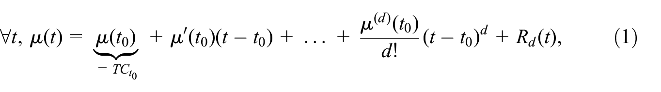
This paper examines and compares real-time estimates of the trend-cycle component using moving averages constructed with local polynomial regression. It enables the reproduction of Henderson’s symmetric and Musgrave’s asymmetric filters used in the X-13ARIMA-SEATS seasonal adjustment algorithm. This paper proposes two extensions of local polynomial filters for real-time trend-cycle estimates: first including a timeliness criterion to minimize the phase shift; second with procedure for parametrizing asymmetric filters locally while they are generally parametrized globally, which can be suboptimal around turning points. An empirical comparison, based on simulated and real data, shows that modeling polynomial trends that are too complex introduces more revisions without reducing the phase shift, and that local parametrization reduces the delay in detecting turning points and reduces revisions. The results are reproducible and all the methods can be easily applied using the R package
1. Introduction
Analysis of the economic cycle, and in particular the early detection of turning points, is a major topic in the analysis of economic outlook. To achieve this, economic indicators are generally seasonally adjusted. However, in order to improve their interpretability, it may be necessary to perform additional smoothing to reduce noise, thereby to analyze the trend-cycle component. By construction, trend-cycle extraction methods are closely related to seasonal adjustment methods, since they are generally applied to seasonally adjusted series.
A moving average, or linear filter, is a statistical method that consists of applying a rolling weighted mean to a times series: for each date
In the last decades, numerous authors proposed methods for the construction of alternative moving averages to derive trend-cycle estimates. In particular, Wildi and McElroy (2019) put forth a model-based approach based on the mean squared error decomposition, while Proietti and Luati (2008), Dagum and Bianconcini (2008), and Grun-Rehomme et al. (2018) proposed non-parametric methods based, respectively, on local polynomial regression, Reproducing Kernel Hilbert Space (RKHS) theory, and minimizing of a weighted sum of moving average quality criteria. All of the aforementioned approaches encompass both Henderson’s symmetric filter and Musgrave’s asymmetric filters. More recently, Quartier-la-Tente (2024) conducted a comparative analysis of these methods by describing a general unifying framework to derive moving averages; Dagum and Bianconcini (2023) provided statistical tests to assess the main properties of the filters defined in terms of revisions and the detection of turning points.
The aim of this study is to propose two extensions to the Proietti and Luati (2008) class of filters in order to take account of two drawbacks of those methods: firstly adding, in the optimization process, a timeliness criterion to directly control the phase shift (i.e., the delay in detecting turning points); secondly calibrating asymmetric filters locally, while they are generally calibrated globally using assumptions that may be wrong locally. Those extensions are implemented in the statistical software R (R Core Team 2022) through the
In Section 2, we describe the general properties of moving averages and the associated quality criteria. This allows us to understand the foundations behind the construction of moving averages from local polynomial regressions, as well as those behind the two extensions proposed in this article (section 3). In Section 4, all these methods are compared empirically on simulated and real series.
2. Local Trend-Cycle Models and Moving Averages
The basic assumption used in time series decomposition methods is that the input observed time series,

where
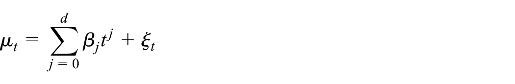
with
Numerous papers describe the definition and the properties of moving averages and linear filters; see for example Ladiray (2018). In this Section we summarize some of the main results to understand the next sections.
Let
When
2.1. Gain and Phase Shift Functions
To interpret the notions of gain and phase shift, it is useful to illustrate the effects of moving averages on harmonic series
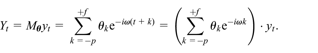
The function

where
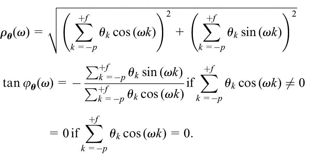
The phase shift is sometimes represented as
To sum up, applying a moving average to a harmonic times series
by multiplying it by an amplitude coefficient
by “shifting” it in time by
Fourier decomposition allows us to analyze any time series as a sum of harmonic series, and each component (trend, cycle, seasonal, irregular) is associated with a set of frequencies. With
Figure 1 shows the gain and phase shift function for the asymmetric Musgrave filter (see Section 3.2) often used for real-time trend-cycle estimation (i.e., when no point in the future is known). The gain function is greater than 1 on the frequencies associated with the trend-cycle
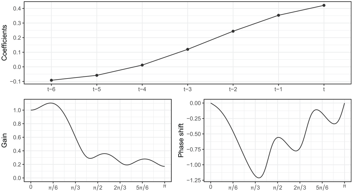
Coefficients, gain, and phase shift function for the Musgrave filter used in X-11 in real-time (last estimate) for monthly series when the bandwidth is 6.
Observed in Figure 1 that for monthly times series, twelve-month cycles (associated to the frequency
2.2. Desirable Properties of a Moving Average
To decompose a time series into a seasonal component, a trend-cycle and the irregular, the X-11 decomposition algorithm (used in X-13ARIMA-SEATS) uses a succession of moving averages, all with specific constraints.
In this paper, we assume that our initial series

The aim will be to build moving averages that best preserve the trend-cycle
Trend-cycles are generally modeled by local polynomial trends (see Section 3) and, in order to best preserve the trend-cycles, we thus design moving averages that preserve the polynomial trends. A moving average
For a moving average
If
2.3. Real-Time Estimation and Asymmetric Moving Average
For symmetric filters, the phase shift function is equal to 0 (modulo
Several approaches can be used for real-time estimation:
Use asymmetric moving averages to take account of the lack of available data;
Apply symmetric filters to an extended forecast series (which is equivalent to using asymmetric moving averages, since forecasts are linear combinations of the past). This method seems to date back to De Forest (1877), which also suggests modeling a polynomial trend of degree 3 or less at the end of the period. A similar approach is used in the X-13ARIMA-SEATS seasonal adjustment method: the series is extended by one year (by default) with an ARIMA model to minimize the revisions associated to asymmetric filters. Since the final filter used for the seasonal adjustment extraction is much longer than one year (in most of the cases, for monthly series, the bandwidth is 78), the input series is just partially extended (and asymmetric filters are still used) to prevent instability over long periods (e.g., outliers or model shifts).
Conversely, the implicit forecasts of an asymmetric moving average can be deduced from a reference symmetric moving average. This allows us to judge the quality of real-time estimates of the trend-cycle and to anticipate future revisions when forecasts are far from expected evolutions.
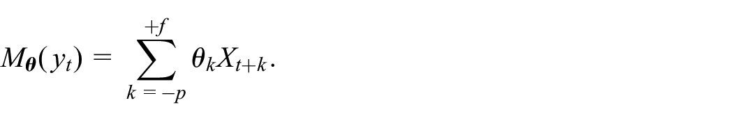
Let us denote
For any integer
In matrix form, this is equivalent to solving:
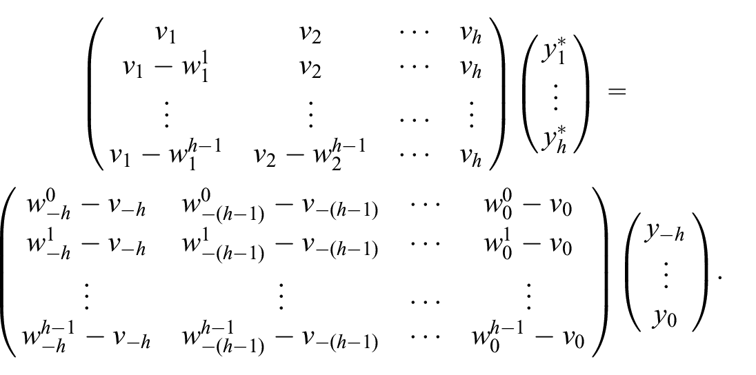
This is implemented in the
As highlighted by Wildi and Schips (2004), extending the series through forecasting with an ARIMA model is equivalent to calculating asymmetric filters whose coefficients are optimized in relation to the one-step ahead forecast. In other words, the aim is to minimize the revisions between the first and last estimates (with the symmetric filter). However, the phase shift induced by the asymmetric filters is not controlled: we might prefer to have faster detection of turning points and a larger revision rather than just minimizing the revisions between the first and last estimates. Furthermore, since the coefficients of the symmetric filter (and therefore the weight associated with distant forecasts) decrease slowly, we should also be interested in the performance of multi-step ahead forecasting. This is why it may be necessary to define alternative criteria for judging the quality of asymmetric moving averages.
3. Non-Parametric Regression and Local Polynomial Regression
Many trend-cycle extraction methods are based on non-parametric regressions, which are particularly flexible because they do not assume any predetermined dependency in the predictors. In practice, local regressions can be used. More specifically, consider a set of points
where
Various estimation methods can be used to derive symmetric and asymmetric moving averages. For example, Gray and Thomson (1996) propose a complete statistical framework that makes it possible, in particular, to model the error in approximating the trend by local polynomials. However, as the specification of this error is generally complex, simpler models may be preferred, such as that of Proietti and Luati (2008). Dagum and Bianconcini (2008) propose a similar modeling of the trend-cycle but using the theory of Hilbert spaces with reproducing kernels for estimation, which has the particular advantage of facilitating the calculation of different moving averages at different time frequencies. See Quartier-la-Tente (2024) for a more detailed comparison of the different recent methods for trend-cycle extraction included in the
In this paper we will focus on Proietti and Luati (2008) approach. Subsection 3.1 and Section 3.2 describes their approach to build symmetric moving averages (used for the final estimates of the trend-cycle component) and asymmetric moving averages (used for real-time estimates). This paper proposed two extensions of their approach to build asymmetric moving averages: a first one adding a criteria to control the phase shift (Subsection 3.4), not used in the simulation (Section 4) but which could be used in future studied; a second one using a local parametrization of a parameter usually parametrized globally (Subsection 3.3), which is used in the simulation.
3.1. Symmetric Moving Averages and Local Polynomial Regression
Using Proietti and Luati’s (2008) framework, we assume that our time series

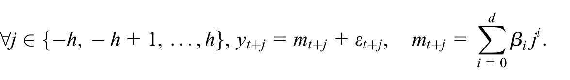
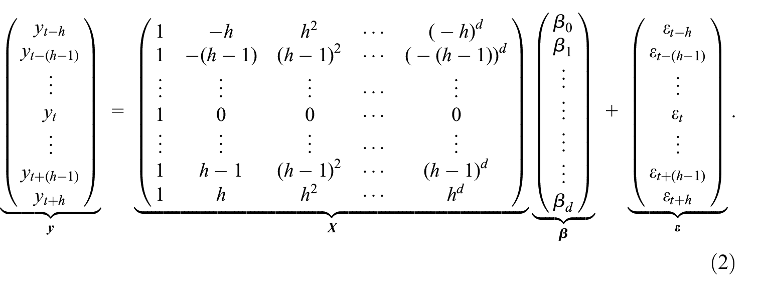
where
The problem of trend extraction is equivalent to estimating
In matrix notation:
Since
where
To conclude, the estimate of the trend
Hence, the filter
Regarding parameter selection, the general consensus is that the choice between different kernels is not crucial. See, for example, Cleveland and Loader (1996) or Loader (1999). The only desired constraints on the kernel are that it assigns greater weight to the central estimation
the degree of the polynomial, denoted by
the number of neighbors
In this paper we will use the Henderson kernel:
However, several other kernels are available in
3.2. Asymmetric Moving Averages and Local Polynomial Regression
As mentioned in Subsection 2.3, for real-time estimation, several approaches can be used:
Apply symmetric filters to the series extended by forecasting
Build an asymmetric filter by local polynomial approximation on the available observations (
Build asymmetric filters that minimize the mean squared error of revision under polynomial trend reproduction constraints.
Proietti and Luati (2008) show that the first two approaches are equivalent when forecasts are made by polynomial extrapolation of degree
To solve the problem of the variance of real-time filter estimates, Proietti and Luati (2008) propose a general method for constructing asymmetric filters that allows a bias-variance trade-off. This is a generalization of Musgrave’s (1964) asymmetric filters (used in the X-11 seasonal adjustment algorithm).
Rewriting Equation (2):
where
where
where
When
When
If the ratio is large
If the ratio is small
Otherwise (most of the cases) a 13-term filter is used and the ratio
When
Linear-Constant (LC):
Quadratic-Linear (QL):
Cubic-Quadratic (CQ):
Supplemental Material shows the coefficients, gain, and phase shift functions of the four asymmetric filters.
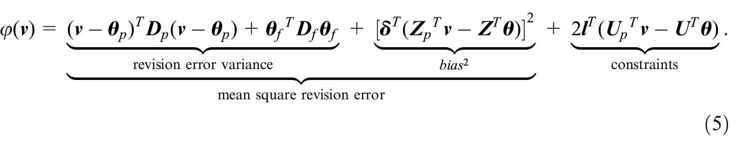
3.3. Extension with the Timeliness Criterion
One drawback of the approach of Proietti and Luati (2008) is the lack of control over the phase shift. However, it is possible to improve the modeling by incorporating in Equation (5) the timeliness criterion defined by Grun-Rehomme et al. (2018). This was proposed by Jean Palate, then coded in Java and integrated into
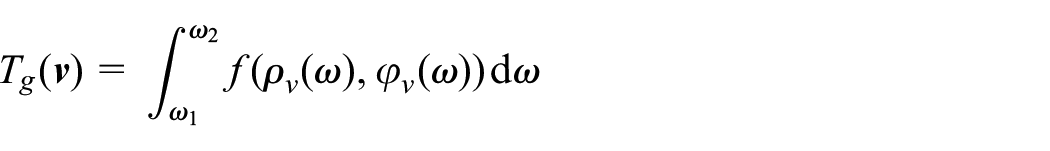
To measure the phase shift between the input series and the filtered one, Grun-Rehomme et al. (2018) introduces a criterion,
As mentioned in Section 2, in the case of trend-cycle extraction we can set

with
Using the same notation as in Subsection 3.2,

Furthermore, the objective function
with
Adding the timeliness criterion:

where
With
One drawback is that
3.4. Local Parametrization of Asymmetric Filters
Asymmetric filters are usually parametrized globally:
This is what is proposed in this article, with a local parametrization of the asymmetric filters by estimating
The variance
Since the symmetric filter is used, only
This is implemented in the function
The parameter
To avoid unrealistic estimates of
For the construction of moving averages, the trend can be modeled as being locally of degree 2 or 3 (this has no impact on the final estimate of concavity). In this paper, we have chosen to model a trend of degree 2: this slightly reduces the phase shift (see Supplemental Material) but slightly increases the revisions linked to the first estimate of the trend-cycle. Figure 2 shows the moving averages used.
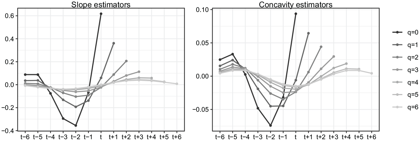
Moving averages used for real-time estimation of slope and concavity.
To distinguish the gain from the local parametrization of the noise associated to the real-time estimates of the slope and concavity, in the empirical applications of Section 4 we also compares the results to the final local parametrization obtained by estimating
Figure 3a: using a symmetric filter to estimate
Figure 3b: using the asymmetric filter which need two points in the future to estimate
The turning points are clearly detected by the local estimators (slope tends toward 0) when
Comparison of the estimates of
There is no function in
4. Comparison of Different Methods
The different methods are compared on simulated and real data. For all series, a symmetric 13-term filter is used: we then assume than the bandwidth is fixed, as in the seasonal adjustment method X-11. A nearest neighbor bandwidth is also tested (13-term asymmetric filters: real-time filter uses observations between
4.1. Simulated Series
4.1.1. Methodology
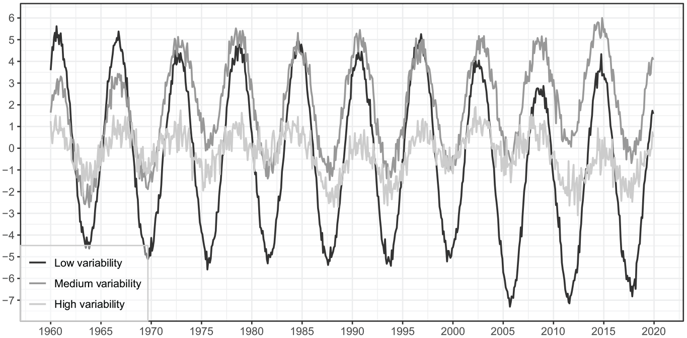
Following a methodology close to that of Darne and Dagum (2009), nine monthly series are simulated between January 1960 and December 2020 with different levels of variability. Each simulated series
the cycle
the trend
and the irregular
For the different simulations, we vary the parameters
High signal-to-noise ratio (i.e., low I-C ratio and low variability):
Medium signal-to-noise ratio (i.e., medium I-C ratio and medium variability):
Low signal-to-noise ratio (i.e., high I-C ratio and high variability):
For each series and each date, the trend-cycle is estimated using the different methods presented in this paper Three quality criteria are computed:
The phase shift in the detection of turning points. In this paper, we focus on turning points associated to business cycle: it is defined as the succession of phases of economic recession and expansion, delimited by peaks (highest level of activity) and troughs (lowest level of activity), see for example Ferrara (2009) for a description of the different economic cycles. In this paper, following Zellner et al. (1991), we used an accepted definition for turning-points:
An upturn occurs when the economy moves from a phase of recession to a phase of expansion. This is the case at date
A downturn occurs when the economy moves from a phase of expansion to a phase of recession. This is the case at date
Let’s denote
Simulated series with low (
In this paper we use a slightly modified criterion: the phase shift is defined as the number of months needed to detect the right turning point without any future revision. Thus, in the case of a downturn, the phase shift is two if
2. The average of the relative deviations between to the last estimate (comparison of the
3. The average of the relative deviations between two consecutive estimates (the
The simulated series are of length sixty years, which is often not realistic for economic time series. However, since all the methods are local, the results are not affected by the length of the series. The length of the series would only have an impact for the identification and the estimation of the ARIMA model. In this case, since the same data generating process is used during the sixty years, it could be relevant to identify the ARIMA model using all the data. Even if it would improve the results in term of phase shift (see Supplemental Material) we prefer to only use the last twelve years to identify and estimate the ARIMA model, to be closer to what would have been done with a real-time series.
4.2. Comparison
Figure 5 represents box plots of the phase shift: the box represents the interquartile range, the central horizontal line represents the median, the dots represents the outliers and the whisker represents the range of the data (if no outlier). For simulated series with medium variability (when a symmetric filter of length 13 is relevant), with the linear constant (LC) method, 50% of the turning point are detected with a phase shift of at most five months whereas when the LC filter is parametrized locally, 50% of the turning point are detected with a phase shift of at most four months. For the direct asymmetric filter (DAF), 25% of the turning are detected with a phase shift of at least seven months (compares to five for the LC method).
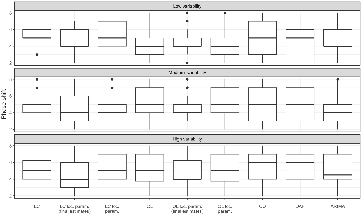
Distribution of phase shift on simulated series.
Excluding for the moment the local parametrizations of the polynomial filters, the linear-constant polynomial filter (LC) seems to give the best results in terms of delay in the detection of turning points. Performance is relatively close to that obtained by extending the series using an ARIMA model. However, when variability is low, the LC filter seems to give poorer results and the quadratic-linear polynomial filter (QL) seems to give the best results.
For series with moderate variability, local parametrization of the LC and QL filters reduces the phase shift. For series with high variability, the phase shift is only reduced by using the final
Observe Table 1 the average of the relative deviations with medium variability. The estimates for
Average of the Relative Deviations of the Revisions for the Different Filters on Simulated Series with Medium Variability.
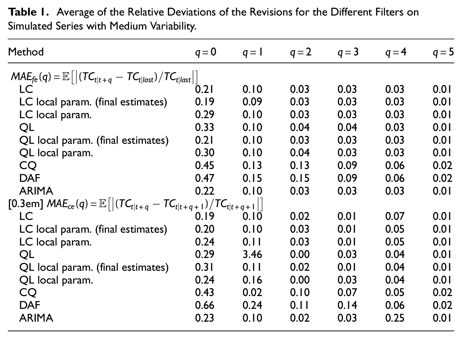
In terms of revisions, the variability of the series has little effect on the respective performances of the different methods, but it does affect the orders of magnitude, which is why the results are presented only for series with medium variability. In general, LC filters always minimize revisions (with relatively small effect from the local parametrization of the filters) and revisions are greater with cubic-quadratic (CQ) and direct (DAF) polynomial filters.
For the QL filter, there is a large revision between the second and third estimates: this may be due to the fact that for the second estimate (when one point in the future is known), the QL filter assigns a greater weight to the estimate in
Extending the series using an ARIMA model gives revisions with the latest estimates of the same order of magnitude as the LC filter, but slightly larger revisions between consecutive estimates, particularly between the fourth and fifth estimates (as might be expected as highlighted in Subsection 2.3).
4.3. Real Series
The differences between the methods are also illustrated using an example from the FRED-MD database (McCracken and Ng 2016) containing economic series on the United States. This database facilitates the reproducibility of the results thanks to the availability of series published on past dates. The series studied correspond to the database published in November 2022. It is the level of employment in the United States (series
Figure 6 shows the successive estimates of the trend-cycle using the different methods studied. For this series, the phase shift is six months for the LC and CQ methods and the extension of the series by ARIMA. It is of two months for the other methods (QL, DAF). In this example, local parametrization does not reduce the phase shift, but it does reduce revisions. The QL and DAF polynomials lead to greater variability in the intermediate estimates, especially in February 2001.
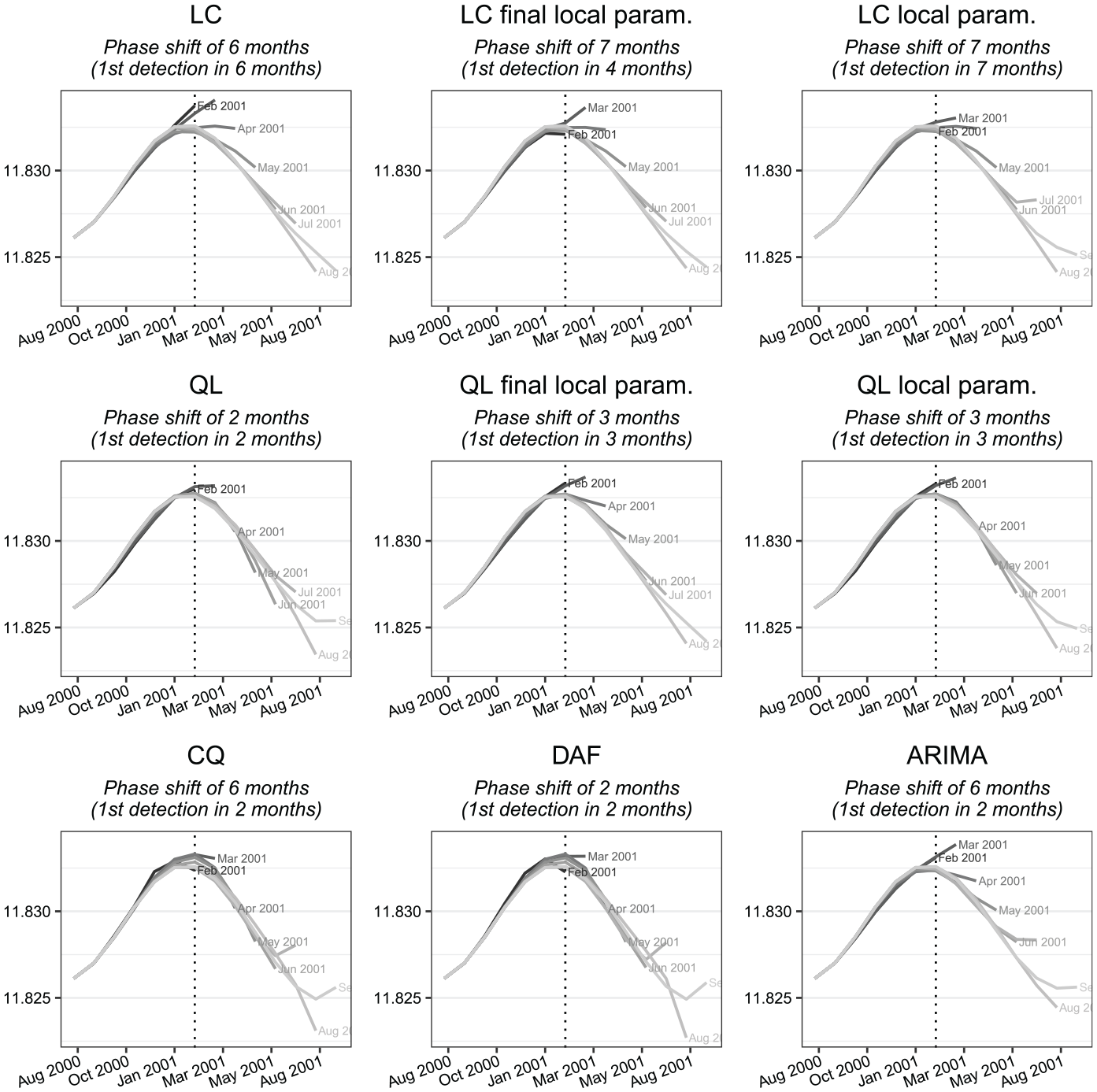
Successive estimates of the trend-cycle in US employment (in logarithms). The dotted vertical line corresponds to the date of the turning point (February 2001). The curve “Feb 2001” corresponds to the estimates of the trend-cycle using the data observed until February 2001. Since a 13-term Henderson filter is used for the final estimates, for the curve “Feb 2001” estimates from September 2001 to February 2001 are intermediate estimates.
The quality of the intermediate estimates can also be analyzed using the implicit forecasts of the different methods (Figure 7). As a reminder, these are forecasts of the raw series which, by applying the symmetric Henderson filter to the extended series, give the same estimates as the asymmetric moving averages. The forecasts of the ARIMA model are naive and do not take the turning point into account, unlike the other methods. Finally, local parametrization of the QL filter produces much more consistent forecasts.
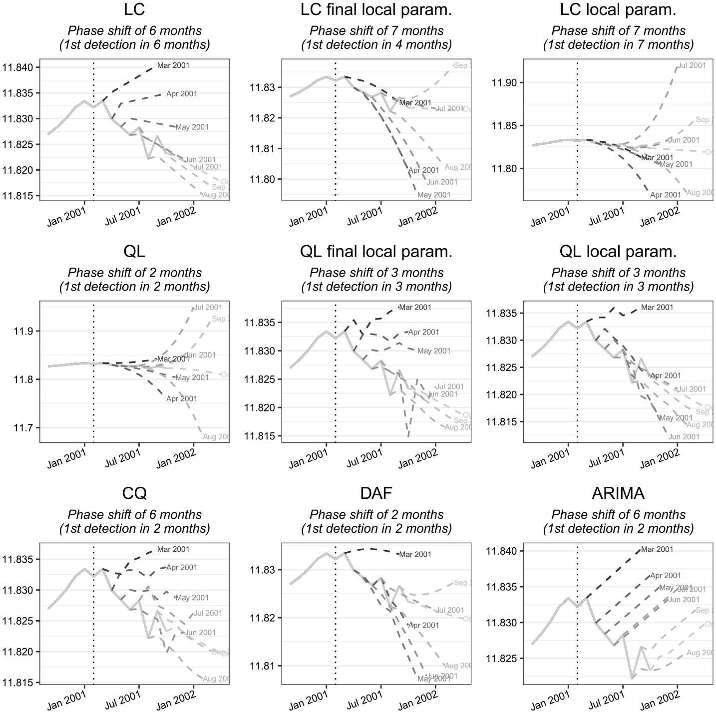
Implicit forecasts linked to successive estimates of the trend-cycle in US employment (in logarithms) using local polynomial methods. The dotted vertical line corresponds to the date of the turning point (February 2001). The curve “Mar 2001” corresponds to the implicit forecasts associated to the asymmetric filters used for the trend-cycle estimations using the data observed until March 2001.
4.4. Discussion
In the Section we discuss the applicability of the presented methods to other frequencies (Subsection 4.4.1) and some limits of the presented methods (e.g., sensitivity to outliers like COVID-19, Subsection 4.4.2).
4.4.1. Other Frequencies
In this paper, we focused on monthly series, but the methods presented can be applied to other frequencies. In general, for lower frequencies, the bandwidth of the symmetric filter reduced. For example, for quarterly series, X-11 uses a 5-term symmetric filter (in general) or 7-term symmetric filter for series with high variability. Mechanically, since fewer points are used, there will be less differences between methods in term of phase shift. For example, on simulated series the results are similar in terms of phase shift but revisions are reduced with local parametrization (see Supplemental Material).
Since X-13ARIMA-SEATS can only be applied for series with frequency lower than monthly, for higher frequencies (weekly, daily, etc.), there is no reference on the length of the filters to uses. The length of the filters can be determined using local polynomial methods, for example minimizing a statistic such as cross-validation (
4.4.2. Outliers and COVID-19
In this article and in those associated to trend-cycle extraction techniques, the moving averages are applied and compared on series already seasonally adjusted or without seasonality (simulated series). The revisions and the phase shift are limited to eight months (when the symmetric filter is thirteen terms) and this has the advantage of isolating the impacts of the different filters from the other processes inherent in seasonal adjustment. There are, however, two drawbacks to this simplification:
The estimation of the seasonally-adjusted series depends on the method used to extract the trend-cycle. The choice of method used to estimate the trend-cycle can therefore have an impact well beyond six months (when a 13-term Henderson filter is used).
As moving averages are linear operators, they are sensitive to the presence of atypical points. Direct application of the methods can therefore lead to biased estimates, due to their presence, whereas seasonal adjustment methods (such as the X-13ARIMA-SEATS method) have a correction module for atypical points. Furthermore, as shown in particular by Dagum (1996), the final symmetric filter used by X-13ARIMA-SEATS to extract the trend-cycle (and therefore the one indirectly used when applying the methods to seasonally-adjusted series), reduces by just 38% cycles of length nine and ten months (generally associated with noise rather than the trend-cycle). The final asymmetric filters even amplify nine and ten-month cycles. This can result in the introduction of undesirable ripples, that is, the detection of false turning points. This problem is reduced by correcting atypical points and the Nonlinear Dagum Filter (NLDF) was defined in this perspective: a. applying the X-11 atypical point correction algorithm (see e.g., Ladiray and Quenneville 2011, for a description) to the seasonally adjusted series, then extending it with an ARIMA model; b. perform a new atypical point correction using a much stricter threshold and then apply the 13-term symmetric filter. Assuming a normal distribution, this amounts to modifying 48% of the irregular values.
The cascade linear filter (CLF), studied in particular in Dagum and Bianconcini (2023), corresponds to an approximation of the NLDF using a 13-term filter and when the forecasts are obtained from an ARIMA(0, 1, 1) model where
Figures 8 and 9 show the successive estimates of the trend-cycle and the associated implicit forecast for the US employment during the COVID-19. First, we observe that while the real turning point is in April 2020, the 13-term Henderson filter produces final estimates of the trend-cycles, biased by the presence of a huge outlier, which lead to a turning point detected in June 2020. Second, as in 2001, the CQ and DAF methods lead to lots of variability in the intermediate estimates. For the QL method, the local parametrization seems to slightly reduce the revisions. For the LC method, local parametrization has little impact on the estimates of the trend-cycle but the associated implicit forecasts are not plausible: the final estimate of the slope is biased by the outlier. Third, the ARIMA model can lead to unrealistic forecasts.
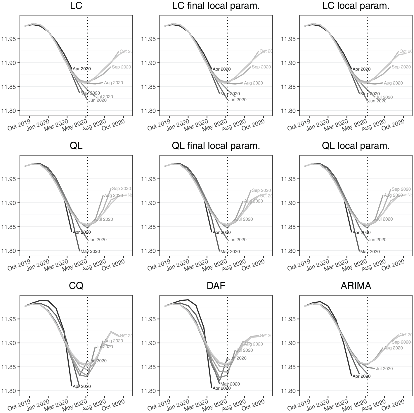
Successive estimates of the trend-cycle in US employment (in logarithms) during the COVID-19.
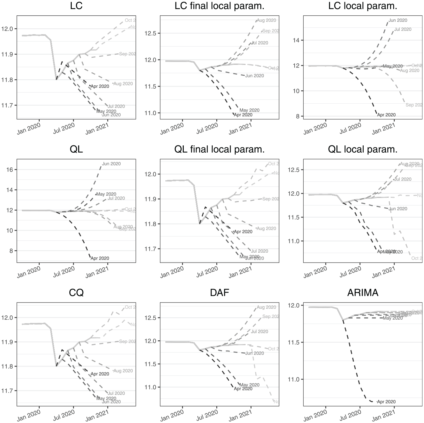
Implicit forecasts linked to successive estimates of the trend-cycle in US employment (in logarithms) using local polynomial methods during the COVID-19.
To sum up, trend-cycle estimates are biased by the presence of outliers which can also impact the detection of turning-points. Several approach could be used to limit their impact of to directly take them into account:
Adjustment of outliers prior to filtering, for example with a RegARIMA model or other correction modules like the one used in X-11.
Increase the bandwidth of the filter used to extract the trend-cycle (it will smooth the trend-cycle by giving less weights to the atypical points).
Since all the filters studied in this paper are equivalent to a local polynomial model, an external regressor can be added to the linear model to handle the outlier (the matrix
Use of robust methods to estimate the trend-cycle, such as robust local regressions or moving medians.
5. Conclusion
For business cycle analysis, most statisticians use trend-cycle extraction methods, either directly or indirectly. They are used, for example, to reduce the noise of an indicator in order to improve its analysis, and models, such as forecasting models, usually use seasonally adjusted series based on these methods.
This paper presents the R package
By comparing the different methods, we can learn a few lessons about the construction of these moving averages.
During economic downturns, asymmetric filters used as an alternative to extending the series using the ARIMA model can reduce revisions to intermediate estimates of the trend-cycle and enable turning points to be detected more quickly.
At the end of the period, modeling polynomial trends of degree greater than 3 (cubic-quadratic, CQ, and direct, DAF) seems to introduce variance into the estimates (and therefore more revisions) without allowing faster detection of turning points. For real-time estimates of the trend-cycle, we can therefore restrict ourselves to methods modeling polynomial trends of degree 2 or less (linear-constant, LC, and quadratic-linear, QL). In addition, parametrizing polynomial filters locally as proposed in this paper enables turning points to be detected more quickly (especially for the QL filter). Even when the phase shift is not reduced, local parametrization is recommended because it reduces revisions and produces intermediate estimates that are more consistent with expected future trends. However, with these methods, the length of the filter used must be adapted to the variability of the series: if the filter used is too long (i.e., if the variability of the series is “low”), retaining polynomial trends of degree 1 or less (LC method) produces poorer results in terms of detecting turning points.
This study could be extended in many ways. One possible extension would be to look at the impact of filter length on the detection of turning points. Asymmetric filters are calibrated using indicators calculated for the estimation of symmetric filters (e.g., to automatically determine their length), whereas a local estimate might be preferable. Furthermore, we have only focused on monthly series with a 13-term symmetric filter, but the results may be different if the symmetric filter studied is longer or shorter and if we study series with other frequencies (weekly or daily, for example).
Another possibility could be to study the impact of atypical points: moving averages, like any linear operator, are highly sensitive to the presence of atypical points. To limit their impact, in X-11 a strong correction for atypical points is performed on the irregular component before applying the filters to extract the trend-cycle. This leads to examining the impact of these outliers on the estimation of the trend-cycle and turning points, and also to explore new types of asymmetric filters based on robust methods (such as robust local regressions or moving medians).
Supplemental Material
sj-pdf-1-jof-10.1177_0282423X241283207 – Supplemental material for Improving Real-Time Trend Estimates Using Local Parametrization of Polynomial Regression Filters
Supplemental material, sj-pdf-1-jof-10.1177_0282423X241283207 for Improving Real-Time Trend Estimates Using Local Parametrization of Polynomial Regression Filters by Alain Quartier-la-Tente in Journal of Official Statistics
Footnotes
References
Supplementary Material
Please find the following supplemental material available below.
For Open Access articles published under a Creative Commons License, all supplemental material carries the same license as the article it is associated with.
For non-Open Access articles published, all supplemental material carries a non-exclusive license, and permission requests for re-use of supplemental material or any part of supplemental material shall be sent directly to the copyright owner as specified in the copyright notice associated with the article.