Sage Journals: Discover world-class research

Abstract

This article provides a new set of empirical regularities describing the U.S. macroeconomy, focusing on business cycle fluctuations in the real GDP and eleven major aggregates from the U.S. National Income and Product Accounts (NIPAs). Patterns of the cyclical fluctuations are assessed using filtering methodologies that adapt to the properties of the series being studied. We employ a recent dataset that includes the Great Recession caused by the 2008 financial crisis and the ensuing recovery. We aim to (1) examine the lead-lag relations via cross-correlations between the aggregate cycle in the U.S. real GDP and the cyclical movements in the eleven major NIPA aggregates; (2) investigate econometrically the inter-linkage between the cyclical component of real GDP and that of each NIPA aggregate by way of the Granger-causality test; and (3) evaluate the capability or the predictive power of each NIPA aggregate to forecast real GDP growth via three forecasting models. Comparisons are made with popular nonparametric HP and Baxter-King (BK) filters. The basic conclusion from the empirical analysis is that the adaptive model-based filters have demonstrated advantages over the commonly used HP and BK filters for business cycle analysis across very diverse economic series from the U.S. national accounts, and the structural time series model using smoothed trend and cycle estimates produced more accurate forecasts than the AR(p) model that forecasts directly using the unfiltered time series.

Keywords

model-based band-pass filters business cycle analysis structural time series modeling

1. Introduction

This article examines a comprehensive dataset from the U.S. National Income and Product Accounts (NIPAs) to investigate the empirical relationships between the aggregate business cycles in the U.S. real GDP and the cyclical movements in eleven major NIPA aggregates. These series represent some of the most widely monitored data on the U.S. economic activity and its breakdown into major sectors. Business cycles are technically defined by co-movements across many sectors. Fluctuations in aggregate GDP are naturally at the center of business cycles, and the cyclical component of real GDP is a useful proxy for the overall business cycle. However, cycles in real GDP and in the major NIPA aggregates exhibit highly heterogeneous dynamics, and thus, an analysis of the complete set of the major aggregates provides useful insights into the diverse behaviors of their cyclical components and their relationships with the aggregate cycles in real GDP.

We employ band-pass filters in order to disentangle cyclical behavior from other dynamics (such as trend and noise) that is present in seasonally adjusted national accounts data, focusing upon two model-based band-pass filters, the Butterworth (BW; Butterworth 1930) and the model-based balanced (BAL; Trimbur and McElroy 2022) filters. BW filters are known for their smooth, monotonically decreasing frequency responses and can be used to construct both low-pass and band-pass filters. Combining two BW filters successively as a low-pass and high-pass filter creates an effective band-pass filter (Pollock 2016). Gómez (2001) demonstrated a model-based interpretation for the BW filters. The model-based BAL filters represent a generalized class of filters based on BW filters, offering flexibility and the ability to extract smooth economic cycles; such filters are implicitly defined by the model and exhibit consistency with each other and the data (Harvey and Trimbur 2003).

Various methods exist for decomposing economic data for business cycle analysis, and Pollock (2016) extensively reviewed these filtering techniques and their statistical properties. They encompass local polynomial regression-based filters like the Henderson filter, finite impulse response (FIR) filters such as the Baxter-King (BK; Baxter and King 1999) and Christiano-Fitzgerald (1998) filters, infinite impulse response (IIR) filters like the Wiener-Kolmogorov filters, which include Hodrick-Prescott (HP) and Butterworth (BW) filters, as well as frequency domain filters. Additionally, there are alternative techniques available like the boosted HP filter, the Hamilton filter, and the Beveridge-Nelson filter, among others (Canova 2020; Celov and Comunale 2023). For this study, we selected the BW filters and the BAL filter due to their smooth frequency responses and adaptability to data, and we discuss their statistical properties and advantages over the HP and BK filters in the following section.

This paper extends the analysis of time series by Stock and Watson (1999) to provide a revised and updated examination of empirical patterns in U.S. business cycle fluctuations using U.S. NIPA data from 1947 to 2018. We consider three relationships (described below) between these NIPA aggregates that each capture separate aspects of their cyclical behavior. Our analysis encompasses the latest macroeconomic data, including the significant Great Recession (GR) in 2008 to 2009. This period represents one of the most impactful business cycle swings in the post-war era. We primarily focus on real GDP and its major components from the U.S. national accounts, as they represent key economic sectors. All data in this study represent real (constant dollar) quantities; because the U.S. NIPAs are compiled with seasonally adjusted data, all empirical investigations are conducted using seasonally adjusted statistics.

Using the trend and cycle estimates from the BW and BAL filters, we aim to investigate the strength of three empirical relationships between the aggregate cycle in real GDP and the cyclical fluctuations in the NIPA aggregates. First, we examine cross-correlations between the cyclical component of real GDP and each of the NIPA aggregates. Cyclical fluctuations can result from various random shocks propagating throughout the economy over time, but their timing and impact on each sector and on the aggregate cycle can vary. Owing to the inconsistent correlations through time and the lead-lag relationships between them, it is not a simple task to define the cyclical relationships between real GDP and the NIPA aggregates merely from the graphs of their cycles. A cross-correlation analysis between the cycle of real GDP and that of each NIPA aggregate provides insights on the lead-lag relationships between them.

Second, we investigate the inter-linkage econometrically via Granger-causality tests (Granger 1969) to determine if the current and past cyclical behavior of an individual NIPA aggregate can predict future cyclical fluctuation in real GDP and vice versa. As a measure of linear dependence between two random variables, cross-correlation tracks the movements of two time series relative to one another at a given lead/lag, whereas Granger causality involves the time dimension and provides a much more stringent criterion for causation. Moreover, correlation is a symmetric object, whereas Granger causality does not need to be symmetric. We employ bivariate autoregressive distributed-lag models for this purpose, allowing us to determine the causal relations between aggregate cycles in real GDP and cyclical fluctuations in each major sector. However, although it is a statistical hypothesis test for determining the causal relations between two time series, Granger-causality test is not a test for predictive power. Granger causality does not imply that using the causing variable will yield better forecasts (this was observed in our study), and it is not uncommon for out-of-sample model selection procedures to disagree with Granger causality.

Third, we assess the capability of an individual NIPA aggregate to forecast growth in real GDP. Real GDP experiences growth and fluctuation simultaneously. Growth, or trend, refers to the long-term movements in the economy, whereas fluctuation, or cycle, refers to repetitive short-term movements that are semi-regular. Thus, models that only use the cycle component to forecast real GDP growth may lead to erroneous forecasts. The estimated trend and cycle embody their respective historical information, and we rely on the consistency of such information in the near future in the forecasting model.

To forecast real GDP growth, we need to consider whether we should directly forecast the GDP series itself, or we are better served by forecasting each component separately. An important advantage of a structural time series model (STM) is its forecasting capability. In a STM, all components are forecasted individually and direct interpretations of each component are possible in the forecast. Moreover, STM forecasting can be viewed as a refinement of the general Granger-causality test, as it allows us to discern the direct impact of a NIPA aggregate on the trend and cycle growth of real GDP and to assess the predictive or forecasting power of each NIPA aggregate.

We consider three models for forecasting real GDP growth. The first model forecasts real GDP growth by separately forecasting the trend and cycle growth before combining them to obtain the growth in real GDP. This allows us to discern the distinct impact of each NIPA aggregate on real GDP growth via its impact on the trend and cycle growth in real GDP. The second model is a single equation model which forecasts real GDP growth using unfiltered series on real GDP and filtered trend and cycle series of a major NIPA aggregate. This model tracks the marginal contributions of current and past GDP growth and the current and past trend and cycle growth of a NIPA aggregate to real GDP growth. The third model is an autoregressive-distributed lag model, which directly forecasts GDP growth using unfiltered data on current and lagged GDP growth and unfiltered data on current and lagged growth of a NIPA aggregate.

We also conducted the three investigations using the HP and BK filtered trend and cycles series to compare the results with those using the trend and cycle series from the model-based BW and BAL filters. All results are computed using Ox and R programming languages.

The paper unfolds as follows: Section 2 examines the statistical attributes of the BW and BAL filters, emphasizing their advantages over the commonly used HP and BK filters for business cycle analysis. It also addresses the statistical fit and model selection for optimal filtering of real GDP and the eleven NIPA aggregates. Section 3 covers the empirical study methods, while Section 4 presents the results. Section 5 summarizes the statistical contributions of the BW and BAL band-pass filters in business cycle analysis and discusses the significance of the empirical findings.

2. Band-Pass Cyclical Filtering

Band-pass ﬁlters have frequently been used to measure the cyclical part of a time series, because they remove both low and high frequency movements while retaining the mid-range frequencies of primary interest for business cycle analysis. By cutting out the low frequency dynamics any trend in the time series is removed, and the resulting ﬁlter output will be stationary (unless forms of non-stationarity other than trends are present). The HP low-pass ﬁlter—popularized by Hodrick and Prescott (1997)—is often used to extract a trend from an economic time series, and subtracting this trend from the original series results in detrended series that has been widely used in business cycle analysis; however, high frequency noise is retained in the cycle estimated with the HP ﬁlter, negatively aﬀecting detection and dating of turning points (Gómez 2001; Hamilton 2018).

Alternatively, band-pass ﬁlters such as those of Baxter and King (1999) produce intermediate periodicities and business-cycle-related ﬂuctuations. These provide—by virtue of high frequency noise elimination—smoother estimates of the cyclical component and clearer information about its trajectory. The BK ﬁlter is a ﬁnite-sample approximation to a so-called ideal ﬁlter, whose stop-band includes all frequencies lower or higher than those associated with the business cycle (usually between two and ten years). This approximation was used by Stock and Watson (1999) to analyze the statistical properties of business cycle movements in macroeconomic time series over the post WWII era from 1947 to 1996. A drawback to the HP and BK filters is that they are sometimes applied without proper reference to the frequency domain structure of the data.

Model-based ﬁlters attempt to extract cyclical eﬀects more accurately by adapting the ﬁlters to the data. Following Trimbur and McElroy (2022), suppose that the observed time series can be written as the sum of three latent independent stochastic processes: a trend µ, a cycle ψ, and an irregular component ι. Time series models are formulated for all three components based on assumptions about the typical behavior of trends and business cycles, as well as idiosyncratic features encapsulated in the irregular component. Then these models are ﬁtted (say, by maximum likelihood estimation) to the data through the model that is implied for their aggregate, and based on these parameter estimates the optimal cycle extraction ﬁlter (Bell 1984) can be constructed—the target “signal” is the cycle ψ, with trend µ and irregular ι composing the “noise.” Hence this model-based filter is attuned to the data; if we approximate the Gaussian likelihood by the Whittle likelihood, we can view this fitting as an alignment of the model spectral density to the periodogram.

In this paper we consider two related classes of model-based band-pass ﬁlters: the Butterworth (BW) ﬁlter and a model-based balanced (BAL) ﬁlter, which Trimbur and McElroy (2022) discuss in detail. The irregular component ι is presumed to be a white noise process, which differs from the BK setting where ι corresponds to high-frequency content. The stochastic cycle is an Autoregressive Moving Average (ARMA) process with cyclical dynamics controlled by parameters for persistency and cyclical frequency; the explicit definition is given in Appendix E of Trimbur and McElroy (2022), where it is shown that the spectral density has a peak in the vicinity of the cyclical frequency (corresponding to a period between two and ten years). Whereas the BAL form is the original formulation of Harvey and Trimbur (2003), the BW form has a simpler expression as an ARMA (2,1) process. Both types of models exhibit cyclical autocovariance functions (see Trimbur 2006), and higher order forms of both BAL and BW exhibit sharper cyclical behavior that results in the model-based cycle extraction filter more closely resembling the ideal band-pass.

The trend µ is assumed to be an integrated autoregressive process of order 1, called a “damped trend”; in the BK setting the trend consists of all frequencies lower than the cyclic frequencies. The HP high-pass filter, in contrast, screens out no high-frequency noise. The HP ﬁlter can be viewed as a noise extraction ﬁlter in a trend-plus-noise model, as discussed by McElroy (2008). In eﬀect, the HP “signal” is ψ + ι rather than ψ.

Extracted trends µ from using BW or BAL ﬁltering are also of some interest. The BK ﬁlter does not provide a direct trend estimate of the trend, but only µ + ι (a trend with high-frequency noise added on) obtained by subtracting the extracted cycle from the data. The HP filter produces a trend via the HP low-pass ﬁlter. In this manner we deﬁne and extract both µ and ψ for any of the extraction methods.

The BW and BAL methods involve cyclical models of a varying order N, as a part of the model speciﬁcation. Higher order cycles correspond to a cyclical extraction ﬁlter that more closely resembles an ideal band-pass shape, since the cutoﬀ of low and high frequencies becomes more pronounced as the order increases. We consider orders between one and eight for both BW and BAL, and apply the BK and HP ﬁlters, for a total of eighteen ﬁlters. (Figure A1-1 to Figure A1-4 in the Appendix shows differences between smoothed cycles of real GDP from BW and BAL filters of order N and N−1, for N = 2, …, 8. As N increases, the differences between filters of N and N−1 quickly diminish.)

The parameters of the BW and BAL ﬁlters are obtained by model fitting, and we select the best models by the Akaike Information Criterion (AIC; Akaike 1976). For the HP ﬁlter, we use the parameter value of 1,600 (recommended for quarterly data). For the BK ﬁlter, the cutoﬀ for the band-pass corresponds to six and thirty-two quarters, or between 1.5 and 8 years. An asymmetric variant (Buss 2010) is used at the beginning and ends of the sample.

The BK and HP filters have the advantage of simplicity, as they can be quickly computed while model-based ﬁlters require model ﬁtting and residual analysis. Nevertheless, we expect the model-based ﬁlters to have superior performance over BK and HP in extracting cycles, because the former are designed to avoid extracting unwanted eﬀects while ensuring cyclical eﬀects that are truly present in the data are retained.

3. The Empirical Study

3.1. Trend and Cycles

The economic series examined in this study are real GDP and eleven NIPA aggregates. The eleven NIPA aggregates include the five major components of real GDP: total consumption, total investment, government spending, export, and imports, as well as the major sub-aggregates of consumption (consumption of durables, nondurables, and services) and major sub-aggregates of total investments (residential and nonresidential investment, and changes of business inventories). The seasonally adjusted quarterly time series in this study spans the period of 1947Q1 to 2018Q2. Historical data are available from U.S. Bureau of Economic Analysis (2018) at https://apps.bea.gov/iTable, and the original data are transformed into logarithmic form.

The smoothed trends and cycles for each series are extracted with the best BW or BAL filters selected with the Akaike Information Criterion (AIC). Table A1 in the Appendix displays the best models for each of the series in the study using a variety of criteria, including AIC and the Schwarz Information Criterion (SIC); however, we focus upon the AIC results, since SIC picked the same model as AIC for eleven out of twelve of the time series. As with the order, the choice of model also varies by series between the BW and BAL filters, with the former being preferred in most cases. The smoothed trend, cycle, and slopes of the trend of real GDP from the third order BW filter, are shown in Figure 1. The shaded regions in the figure are the NBER-determined recessions. Aggregate fluctuations are clearly more pronounced in the detrended—or the smoothed cycle—series. Trend, slope of the trend, and the cycles of each NIPA aggregate are available in the Supplemental Materials.

Figure 1.

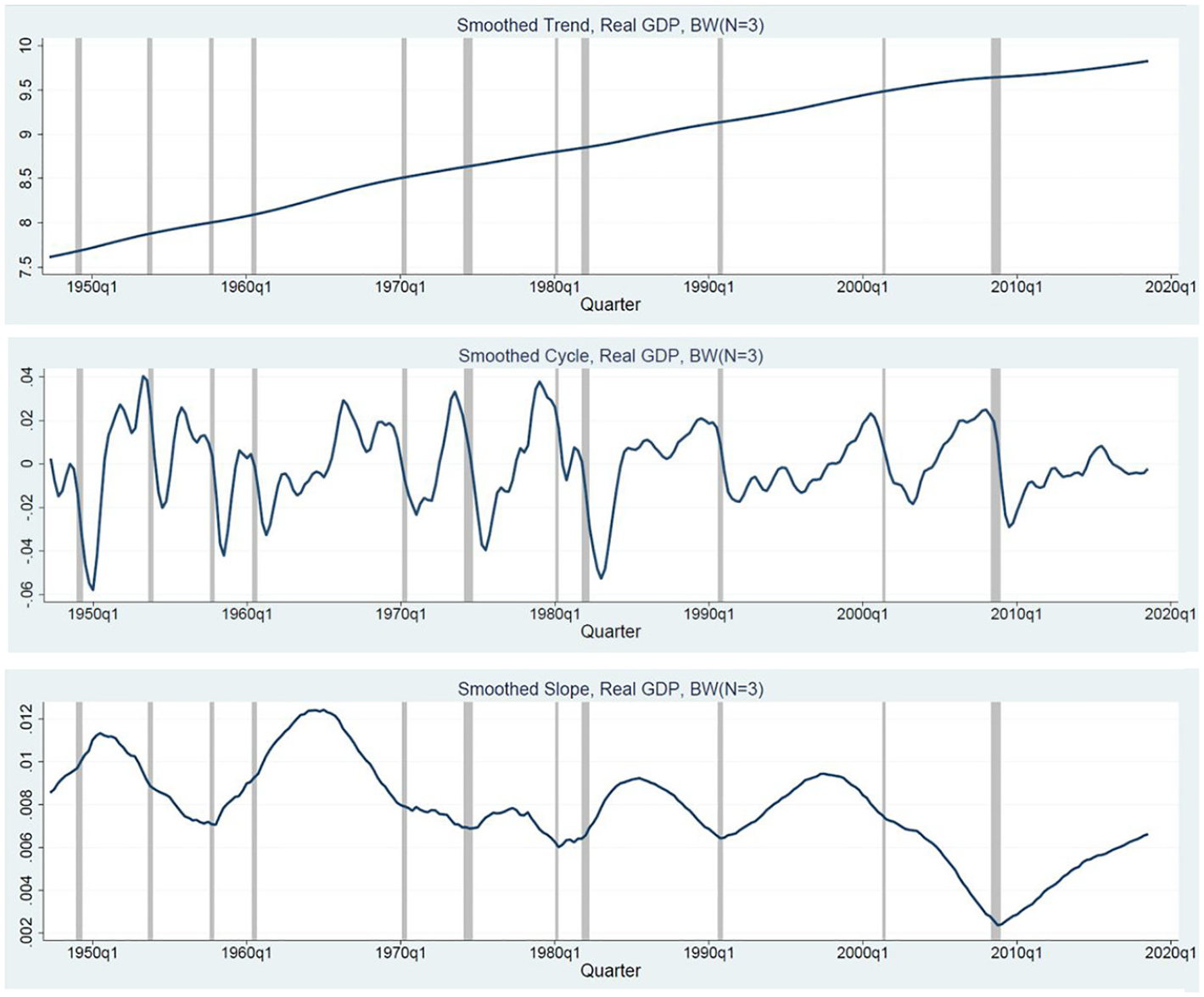
Quarterly estimates, smoothed trend, cycle, and slope of the trend of real GDP, 1947 to 2018.

The varying dynamics of real GDP and the NIPA aggregates can be depicted by comparing the smoothed cycles of real GDP paired with one of the eleven NIPA aggregates extracted with the best BW or BAL filters selected for the series. It is intuitive, as shown in Figure 2a and b, that unlike the consumption of services, which has a noisier cycle (i.e., a lower order stochastic cycle), real investment has a very pronounced cycle (i.e., a higher order cycle). Shaded areas in the figures indicate the NBER defined business recessions. Also see Figures A2-1 to A2-9 in the Appendix for smoothed cycles of other NIPA aggregates compared with the aggregate cycle of real GDP. Evidently, the dynamics of the aggregate cycles of real GDP and the cyclical movements of the NIPA aggregates can be quite different.

Figure 2.

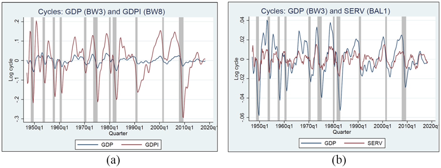
(a) Smoothed cycles of real GDP (BW3) and real investment (BW8) and (b) smoothed cycles of real GDP (BW3) and consumption of services (BAL1).

To compare the smoothed cycles from different filters, Figure 3a and b and Figures A3-1 to A3-10 in the Appendix depict the smoothed cycles of real GDP and that of each NIPA aggregate extracted with the selected BW or BAL filter with the smoothed cycles extracted with the HP and BK filters. Noticeably, cycles of durable goods (DUR) and cycles of exports (EXP) extracted with the HP filter are consistently noisier, exhibiting greater short-term variations. Similar noisiness of the cycles extracted with the HP filter are noticeable from Figures A3-1 to A3-10. Because BK provides a finite approximation of the ideal filter, the quarterly series extracted with the symmetric BK filter are truncated by twelve quarters at both ends of the sample.

Figure 3.

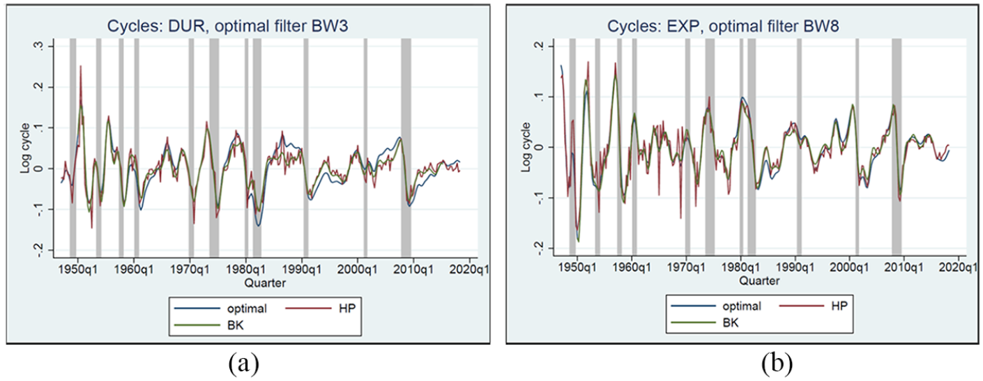
(a) Smoothed cycle of DUR from selected filter BW3 and the HP and BK filters and (b) smoothed cycle of EXP from selected BW8 and the HP and BK filters.

3.2. Cross-Correlations

Business cycles are technically defined by co-movements across many sectors in an economy, yet aggregate fluctuations in real GDP are at the center of business cycles. Thus, the cyclical component of real GDP is considered a benchmark for comparison across its major component series. Real GDP and the major NIPA aggregates have different statistical properties and exhibit diverse dynamics. Aggregate cyclical fluctuations can be caused by national or even global shocks, but the timing of such shocks and the severity of the impacts on the aggregate cycles in real GDP could differ from those experienced in different sectors in the economy.

However, it is not a simple task to define the relationships between the cycle of real GDP and that of each NIPA aggregate by viewing the graphs of the cycles. To understand their diverse properties, we first examine the cross-correlations to investigate whether cyclical movement in an individual NIPA aggregate leads or lags the aggregate cycles. Specifically, Corr( $y_{t}, x_{t + k})$ measures cross-correlation between smoothed cycles of real GDP at time $t, y_{t}$ , and the $k$ –quarter lead of the smoothed cycles of a NIPA aggregate, $x_{t + k}$ . In other words, Corr( $y_{t}, x_{t + k})$ measures the correlation of the cycles of a NIPA aggregate against the aggregate cycles in real GDP. The correlation at $k$ = 0 indicates contemporaneous correlation. A large positive correlation at $k$ = 0 indicates procyclical behavior of the NIPA aggregate series, and a large negative correlation at $k$ = 0 indicates counter-cyclical behavior of the NIPA aggregate series. The largest correlation in absolute terms determines the lead-lag property of a given series relative to another. For example, a maximum correlation occurring at $k$ = −1 indicates that the cycles of a NIPA aggregate series tend to lag the aggregate cycles in real GDP by one quarter. We report and compare the cross-correlations between real GDP and each NIPA aggregate computed using cycles extracted from the best BW and BAL filters as well as the HP and BK filters.

3.3. Granger-Causality Tests

Our second task is to use the Granger-causality test to investigate whether there is sufficient statistical evidence that the cyclical movement of a NIPA aggregate has a causal effect on the cycle of real GDP and vice versa. Note that the existence of such a causal relationship between an index (real GDP) and its component (a NIPA aggregate) is not a necessity; the functional relationship of these two series is instantaneous, whereas here we investigate lagged relationships of their respective extracted cycles. In this study, we report pairwise Granger-causality tests, as we focus on the Granger-causal relations between the cyclical behavior of an individual NIPA aggregate, $x$ , and the aggregate cycles in real GDP, $y$ .

To examine Granger causality between $x$ and $y$ , the hypotheses tested are whether the parameters governing the effects of lagged $x$ and $y$ respectively on $y$ and $x$ are zero. If both hypotheses are rejected, then there is a “feedback” relation between $x$ and $y$ . If the former hypothesis is rejected but the latter is not, then there is unidirectional causality running from $x$ to $y$ , whereas if the latter is rejected and the former is not, the reverse is true. See Granger (1969) for the statistical formulation of the tests. For Granger-causality tests, one approach is to specify a fixed lag-length structure. However, because of the diverse properties of the NIPA series, we choose to identify the lag length of each test based on AIC. The Granger-causality tests were conducted using smoothed cycle series extracted with the best BW and BAL filters. The test results are compared with those using smoothed cycles extracted with the HP and BK filters.

3.4. Forecasting Real GDP Growth

Real GDP is growing and fluctuating at the same time. A trend represents the long-term movements of the economy, and cycles reflect the short-term movements of the economy with some regular behaviors repeated over time. When modeling GDP time series, there are two important aspects to consider with. First, how well the model explains the actual data, and second, how well the model forecasts the economy at various horizons. In a STM, all components in the model are forecasted individually, and direct interpretations of the forecasts for each component are also possible. As we focus on the relationships between the aggregate cycles in real GDP and the cyclical fluctuations in the major NIPA aggregates, a proper choice of trend is necessary to ensure appropriate forecast of the cyclical component.

The structural time series framework constructed to develop the model-based BAL filter chooses a damped smooth trend with a stochastic slope. The BW low-pass filter is equivalent to a trend extraction in a stochastic trend plus noise model. By introducing the damping factor that allows the cycle to be stationary, a more general class of the BW band-pass filters is defined. Setting up a model with both a trend and a cycle leads to a class of generalized BW filters that extract trend and cycles in a mutually consistent manner (Harvey and Trimbur 2003).

To forecast real GDP growth, the first question to consider is whether we should forecast real GDP growth directly using unfiltered data, or we are better served to use filtered trend and cycle series for forecasting. The second question is whether in a STM we should first separately forecast the trend and cycle growth before combining them to obtain the forecast of GDP growth, or we should forecast real GDP growth in a single equation model which traces the marginal contributions of trend and cycle components of a NIPA aggregate to real GDP growth. We consider three models to find answers to these two questions.

We examine the ability of an individual NIPA aggregate to forecast real GDP growth; hence, these forecasting exercises refine the general Granger causality tests, as our forecasting models allow us to discern the direct impact of a NIPA aggregate on the growth in trend and cycle components of real GDP and allow us to examine the results over various forecasting horizons.

We denote the logarithm of real GDP by $y_{t}$ and the logarithm of a NIPA aggregate by $x_{t}$ . We denote trend, cycle, and irregular parts with subscript $y$ , $x$ for GDP and a NIPA aggregate. The structural time series model for $y_{t}$ is

y_{t} = μ_{y, t} + ψ_{y, t} + ι_{y, t}

(1)

We forecast the model $k$ quarters ahead, where $k = 1, 4, 8$ . For model $j = {A, B, C}$ , we denote the forecast of real GDP growth by $Δ {\hat{y}}_{t + k}^{j}$ , where $Δ$ denotes the temporal difference.

Model A: This is a two-step method to forecast real GDP growth. In the first step, we estimate two separate equations, one predicting $k$ -step ahead trend growth, $Δ μ_{y, t + k}$ as a function of current and lagged growth of the trend of real GDP and those of a NIPA aggregate, and one predicting $k$ -step-ahead cycle growth $Δ ψ_{y, t + k}$ as a function of current and lagged growth of the cycle of real GDP and those of a NIPA aggregate. Let $l^{μ}$ and $l^{ψ}$ be the lag lengths in our equations. The first equation is for forecasting GDP trend growth, where $\hat{E}$ denote the forecast of the variable in [.],

\hat{E} [Δ μ_{y, t + k}] = \sum_{s = 0}^{l^{μ}} α_{μ, s}^{(A)} Δ μ_{y, t - s} + \sum_{s = 0}^{l^{μ}} β_{μ, s}^{(A)} Δ μ_{x, t - s}

(2)

and the second equation is for forecasting GDP cycle growth,

\hat{E} [Δ ψ_{y, t + k}] = \sum_{s = 0}^{l^{ψ}} α_{ψ, s}^{(A)} Δ ψ_{y, t - s} + \sum_{s = 0}^{l^{ψ}} β_{ψ, s}^{(A)} Δ ψ_{x, t - s}

(3)

Finally, we compute forecast of GDP growth rates as combined forecasts of the trend and cycle growth,

\hat{E} [Δ y_{t + k}^{A}] = \hat{E} [Δ μ_{y, t + k}] + \hat{E} [Δ ψ_{y, t + k}]

(4)

Model B: This is a single equation model to forecast GDP growth based on both current and past data on the growth of $y$ based on the unfiltered data and current and lagged trend and cycle growth of $x$ . We set the same lag length $l$ for all variables.

\hat{E} [Δ y_{t + k}^{B}] = \sum_{s = 0}^{l} γ_{s}^{(B)} Δ y_{t - s} + \sum_{s = 0}^{l} β_{μ, s}^{(B)} Δ μ_{x, t - s} + \sum_{s = 0}^{l} β_{ψ, s}^{(B)} Δ ψ_{x, t - s} .

(5)

Model C: This is an autoregressive distributed lag model to forecast real GDP growth using unfiltered time series on real GDP and unfiltered time series on a NIPA aggregate,

\hat{E} [Δ y_{t + k}^{C}] = \sum_{s = 0}^{l} α_{s}^{(C)} Δ y_{t - s} + \sum_{s = 0}^{l} β_{s}^{(C)} Δ x_{t - s} .

(6)

We can also estimate the three models by restricting the β coefficients on the $x s$ to zero and label such forecasts $Δ {\tilde{y}}_{t + k}^{j}$ . This produces the forecast using the “restricted model,” that is, with no contribution from $x$ , while $Δ {\hat{y}}_{t + k}^{j}$ is a forecast using an “unrestricted model,” which allows the contribution from the NIPA aggregate $x$ . If forecasts from the restricted and unrestricted models are statistically indistinguishable, then we fail to reject the null hypothesis that $x$ does not help forecast growth in $y$ .

Under the restricted Model A, the growth in real GDP depends on the dynamic changes in the trend and cycle of real GDP alone. Because Model B uses unfiltered data on real GDP growth and smoothed estimates on the trend and cycle growth of a NIPA aggregate, and Model C uses unfiltered series on both real GDP and a NIPA aggregate, the restricted Model B and Model C are identical, where forecasts of real GDP growth depend only on unfiltered time series on real GDP. This case corresponds to a dynamic regression of the index on its own past alone, which might be viewed as a plausible benchmark forecasting model; the unrestricted schemes, in contrast, incorporate information from other NIPA aggregates (through cycles and trends), and therefore are reasonable candidates to provide forecast improvements. In summary, we have three unrestricted and two restricted models to evaluate the ability of each NIPA aggregate to forecast real GDP growth.

In-sample estimation and pseudo-out-of-sample (POOS) forecasts: Ideally, we would want to compute forecasts conditional only on current and past information. However, estimating trend, cycle, and irregular components for forecasting based only on sample information up to the current period is not always feasible, because that would require filtering data for each POOS forecast. To keep the computational work manageable, we filter the data once using the full sample, treating the filtered trend, cycle, and irregular series as if they were actual data. We filtered the data using the BW and BAL filters selected for real GDP and for the eleven NIPA aggregates as well as the BK and HP filters. We divide the full filtered sample into estimation sample and testing sample for the POOS forecasts. As we are interested in the ability of each model to forecast real GDP growth using data before and after the GR, we constructed two estimation samples. The first estimation sample spans the period 1947Q1 to 1997Q4, and the second estimation sample spans the period 1947Q1 to 2007Q4.

We estimate each of the five models using the estimation samples to obtain estimates of coefficients, and then compute the $k$ -step POOS forecasts based on the estimated models, with $k$ = 1, 4, 8 for the duration of the testing sample. We choose recursive estimation based on an expanding data window to compute the predictions, so that each POOS prediction is computed based on the estimated model with all observations $k$ quarters prior to the quarter to be predicted.

We set the first testing sample for POOS forecasts to cover the period of 1998Q1 to 2007Q4 and the second testing sample to cover 2008Q1 to 2017Q4. The first set of forecasts covers the ten-year period prior to the GR, and the second set of forecasts covers ten years following the GR. For each model, we examine the ability of each of the eleven NIPA aggregates to forecast real GDP growth. Thus, there are eleven sets of forecasts for each of the three unrestricted and two restricted models, using two estimation and testing samples for each forecasting horizon, totaling 990 sets of estimated coefficients and forecasts.

We evaluate the forecasting performances of each model in terms of root mean squared forecasting error (RMSFE). We also conducted the Diebold-Mariano (DM) test to compare the predictive accuracies of the unrestricted and restricted models for a given filtering technique, and the predictive accuracies using smoothed data from different filters for a given model. However, there are some technical challenges in making such comparisons. First, the BK filter is designed to generate filtered cycle series that do not contain fluctuations at higher or lower frequencies than those of the business cycles. As such, the BK filter does not produce the filtered trend series. Thus, it is difficult to estimate the first two models and compute POOS forecasts with the BK filtered series. One option is to only compare the forecasts of cycle growth across filtering techniques using Model A. Alternatively, we can back out a trend consistent with the BK filter by using the spectral gain to the left of the pass-band, that is all the frequencies below the lowest one passed by the BK filter. We chose the second alternative in order to have a complete comparison. Moreover, since the symmetric BK filter is unable to extract the band of frequencies at both ends of the sample, multiple sample observations are truncated at the ends of the series in the real time estimation. To avoid such a problem, we adopted an extension to an asymmetric BK filter: the optimal correction scheme of the ideal filter weights is the same as in the symmetric version—cut the ideal filter at the appropriate length and add a constant to all filter weights to ensure zero weight on zero frequency. The extension to an asymmetric filter is useful whenever real time estimation is needed. The developed filter can be used in any field of science where it is necessary to extract a band of frequencies from a signal (Buss 2010).

Another technical challenge is in comparison with the HP filter. The HP filter is often used to remove the cyclical component of a time series from raw data. It is designed to obtain a smooth representation of the time series, which is more sensitive to long-term than to short-term fluctuations. Because the HP filter does produce filtered trend and cycle series, we could compare the forecasting performances using the HP filtered trend and cycle series with those using the trend and cycle series from other filters.

Finally, as pointed out in various studies, there is high frequency noise in the cycles filtered with the HP filter, and the HP may be inappropriate for some time series (Gómez 2001; Hamilton 2018; Mohr 2005). As noted above, the visible noisiness of the HP filtered cycles series are shown in Figure 3a and b in Section 3.1 and in Figures A3-1 to A3-10 in the Appendix. The comparison of Model A and Model B with series extracted with the HP, the BK, and the selected BW and BAL filters could provide some insights into the ability of decomposed trend and cycle series using alternative filtering technique for forecasting real GDP growth.

4. Results from the Empirical Study

4.1. Patterns of Cross-Correlations

Cross-correlations, Corr( $y_{t}, x_{t + k})$ , of the cyclical component of each NIPA aggregates against the aggregate business cycles proxied by the cyclical component of real GDP, are computed using cycles filtered with (1) the best BW or BAL filter for real GDP and each NIPA aggregate based on AIC; (2) the HP filter; and (3) the BK filter. We report cross-correlations for $k$ = −10, −9, …, 0, 1, 2, …, 10 in Table A2 in the Appendix. Column 3 in Table A2 reports the standard deviation of the cyclical component of each NIPA aggregate. Because all series, except the change of business inventories, are in logarithmic form, the standard deviations for these series measure the percentage deviations from the trend growth paths, and thus, are comparable across series. Change of business inventories, which can be positive or negative, is computed as the ratio of the native units to real GDP, and the standard deviation yields the percentage deviation from the relative trend of the two series.

The best filters selected for real GDP, total consumption, consumption of durables, nondurables, and services are BW3, BW8, BW3, BW2, and BAL1, respectively. High positive cross-correlations at lag $k$ = 0 of cycle series from all four filters indicate strong procyclical behaviors for all consumption aggregates. The maximum cross-correlations of 0.80 and 0.70 at $k$ = 1 indicate that total consumption and consumption of durables are procyclical with a one-quarter lead of the aggregate cycles of real GDP, whereas the maximum cross-correlations of 0.74 and 0.71 at $k$ = 0 suggest that the cycles of consumption of nondurables and services move coincidently with the aggregate cycles.

As shown in Figure 2b and Figures A2-1 to A2-3 and the standard deviations tabulated in Table A2, the cyclical component of consumption of services exhibits the lowest dispersion (Stdv. = 0.52) and is considerably smoother than the cyclical component of real GDP. The cyclical component of consumption of nondurables is moderately more dispersed than that of consumption of services, but less so than the aggregate cycles of real GDP. In contrast, consumption of durables is strongly procyclical and far more volatile (Stdv. = 5.29) than aggregate GDP and the other consumption measures. The lead-lag relationships indicated by the cross-correlations and the measured dispersions are consistent with the observed smooth consumption of nondurables and services throughout business cycles as implied by the permanent income hypothesis. In contrast, the one-quarter lead in cross-correlation and the high volatility in the cycles of consumption of durables reflect the high sensitivity of such consumption to the changing economic conditions, as the expectations of changing economic conditions often affect the decisions on such consumption.

Cross-correlations for real GDP and the four consumption measures computed from the HP and BK filtered cycles are consistent with those from the selected BW and BAL filtered cycles, except for the total consumption cycle from the HP filter. Instead of the one-quarter lead of the aggregate cycle, the much noisier consumption cycle from the HP filter exhibits coincidental movement with the aggregate GDP cycles.

The best filters selected for total real investment, residential, nonresidential, and change of business inventory investment are, respectively, BW8, BAL2, BW2, and BAL8. The BW8 and BAL8 filters as the best filters, respectively, for extracting smoothed cycles of total real investment and change of business inventories suggest that more high frequency noise need to be filtered out to extract the smoothed cyclical component from the raw time series of these investment measures. Positive correlations at $k$ = 0 indicate procyclical behaviors of the investment series extracted from all filters. The maximum correlation of 0.74 at $k$ = 0 indicates that cycle of total investment moves coincidently with the aggregate cycle in real GDP. However, the maximum correlation of 0.62 and 0.78 occurring at $k$ = 2 and $k$ = −1, respectively, for residential and nonresidential investment indicate that residential investment is procyclical with a two-quarter lead of the aggregate cycle as shown in Figure 4a, whereas non-residential investment is procyclical with a one-quarter lag of the aggregate cycles. The correlations computed with the HP and BK filtered cycles reveal the same lead-lag relationships between the cyclical movements of these three investment measures and the aggregate cycles of real GDP.

Figure 4.

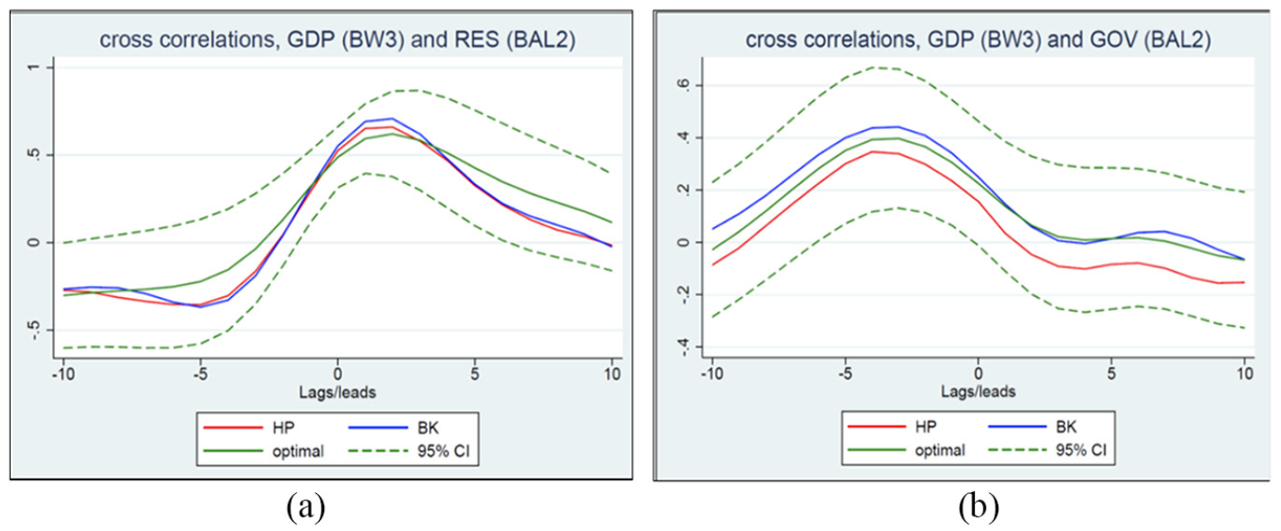
(a) Cross-correlation between cycles of real GDP and cycles of residential investment and (b) cross-correlation between cycle of real GDP and cycles of government spending.

The cyclical component of residential investment is the most volatile of the four investment measures (Table A2: Stdv. = 13.78) and of the NIPA aggregates. The highly volatile cyclical behavior and the two-quarter lead of the aggregate cycle reflect the highly sensitive investment behavior in this sector in response to anticipated changes in the economic conditions (Green 1997).

Nonresidential investment, on the other hand, includes firms’ purchases of capital goods and the construction of factories and commercial buildings. Such investment will respond to changes in the economic conditions, but it is less flexible to adjust quickly to the changes in the economic conditions (Fisher 2007; Green 1997; Kliesen 2016).

Cycles of change in business inventories move with a one-quarter lead of the aggregate cycle in real GDP based on the selected BAL filter. This one-quarter lead relationship is supported by empirical observations that inventory investment provides a consistent lead in overall business activities, and thus, is retained as part of the U.S. composite index of leading indicators to gauge future economic conditions. In contrast, cycles of change of business inventory from HP and BK filters move coincidentally with the aggregate cycles in real GDP.

As shown in Figure 4b, government expenditures exhibit very weak correlations with the aggregate cycles in real GDP with correlations between 0.16 and 0.25 at $k$ = 0 based on the cycles from all filters. The low correlations are perhaps because government expenditures are primarily driven by policy decisions. Moreover, cyclical movements in government spending are shown to have a three-quarter lag based on the BAL and BK filtered cycles and a four-quarter lag based on the HP filtered cycles, consistent with the observations that government expenditure has often been used to stimulate the economy during recessions but implementation of such polices come with a delay.

For imports, the maximum correlations between 0.71 and 0.79 at $k$ = 0 computed with cycles from all filters indicate that imports are highly procyclical and move coincidently with the aggregate cycles in real GDP. Empirically we observe that the imports fall during an economic downturn and rise in a booming economy as personal income changes through the business cycle. For exports, moderate correlations between 0.29 and 0.42 at $k$ = 0 indicate a mildly procyclical relationship with the aggregate cycle, consistent with the statistically supported lesser dependency between the foreign sector and GDP in the U.S. (Zestos and Tao 2002). Moreover, exports are shown to be procyclical with real GDP but with a two-quarter lag based on the BW and BK filtered cycles and a one-quarter lag based on the HP filtered cycles. Intuitively, businesses usually cut back on production during a recession, which can lead to a decrease in exports. As adjustments in production take time, changes in exports in response to changes in economic conditions come with a delay (Stock and Watson 1999). Furthermore, exports can also be affected by the value of the currencies, which could be driven by monetary policy and global economic conditions (Zestos and Tao 2002). The cycles of exports and imports are depicted in Figures A2-8 and A2-9. Cyclical components of exports and imports are more volatile than those of real GDP and the consumptions aggregates but are less volatile than the cyclical components in total and residential investment.

Cross-correlations between aggregate cycles of real GDP and the cycles of the remaining nine NIPA aggregates computed using the BW and BAL filters as well as the HP and BK filters are compared in Figure A4 in the Appendix. The 95% confidence intervals for the cross-correlations computed from the best selected filters are included in the figures. Correlations based on the cycles from the BW or BAL filters and those from the HP and BK filtered cycles are noticeably different. Moreover, the HP and BK filtered cycles tend to have much lower correlations at longer leads and longer lags.

4.2. The Granger-Causal Relations

The pairwise Granger-Causality tests were conducted using smoothed cycles from the selected model-based filter for each series and the HP and BK filters. We chose to allow a maximum number of lags for the dependent and independent variables in the bivariate autoregressive distributed-lag model determined by the smaller of T−1 and 10*log₁₀(T−1) with T being the number of quarters of the data series and select the lag-order in each pairwise Granger-causality test based on the information criterion AIC. Table A3 in the Appendix displays the test results between real GDP and each NIPA aggregate.

Degrees of freedom displayed in the column labeled “DF(AIC)” in Table A3 indicate the lag-order in each pairwise Granger test based on AIC. Evidently the varying lag-order selected in each test depends on the dynamic characteristics of the cycle series, and the lag-order selection can be affected by the filter used to extract the cycle series. In the bivariate Granger tests, the cyclical component of real GDP, $y$ , and that of the NIPA aggregate, $x$ , are the jointly determined endogenous variables. The null hypotheses for the pairwise Granger-causality test are that the cyclical movement of a NIPA aggregate does not Granger-cause aggregate cyclical movement in real GDP and vice versa. The Chi-square statistics and the p-values for each test are reported in Table A3. We did not adjust these p-values for multiple comparisons, since there are many types of multiple comparisons that could be contemplated, for example, across the three filter types, or including forward and backward causality, or across NIPA aggregates, etc. To make the results the most widely accessible for different user interests, we do not make this adjustment.

For the four consumption aggregates, both null hypotheses are strongly rejected based on the tests using cycles extracted with the selected BW and BAL filters and the HP filter, suggesting strong “feedback” causal relations between aggregate cycles in real GDP and the cyclical fluctuations in each consumption aggregate. However, the Granger tests based on the BK-filtered cycles suggest only the unidirectional Granger-causal relations running from real GDP to the consumption of durables and nondurables. Moreover, the tests based on the BK-filtered cycles also suggest that aggregate cycles in real GDP do not Granger-cause cyclical fluctuations in total consumption and consumption of services. These results based on the BK filtered cycles seem inconsistent with the empirically observed feedback relations between the consumptions aggregates and real GDP.

For four investment aggregates, both null hypotheses for the Granger-causality tests using estimated cycles from the selected BW and BAL filters are strongly rejected, indicating strong feedback in the Granger-causal relations between the aggregate cycle in real GDP and the cyclical movements in the investment aggregates. Such results are strongly supported by the empirical observations that the two largest investment sub-aggregates—residential and nonresidential investments—are procyclical with strong feedback relation with real GDP (Fisher 2007; Green 1997; Kliesen 2016).

For the investment aggregates, the Granger-causality tests using the BK and HP filtered cycles show consistent results with those based on the cycles from the selected BW and BAL filters, except that the Granger test based on the HP filtered cycles suggested only a unidirectional Granger-causal relation running from real GDP to total investment. Such a conclusion contradicts the test results of the three major investment sub-aggregates and is inconsistent with the observations that increases in investments tend to boost the economy.

The Granger tests based on the estimated cycles from the selected model-based and the BK filters concluded the strong “feedback” causal relations between the aggregate cycle of real GDP and the cyclical movement in the government spending, whereas the tests based on the HP filtered cycle concluded a unidirectional causal relation running from government spending to real GDP and not vice versa. These results support the empirical observation that government spending has often been used to stimulate the economy during economic downturns. Intuitively, during periods of strong economic growth, there is less rationale to increase government spending, as suggested by the test results based on the HP filtered cycles. Obviously, there are other political factors that may impact the cyclical patterns of government spending (Nyasha and Odhiambo 2019).

The Granger tests using cycles from all filters conclude the “feedback” Granger-causal relations between the aggregate cycle in real GDP and the cyclical movement in exports at least at the 5% significance level, which confirm the intuition that rising exports will lead to higher economic growth, and growth in exports can also have knock-on effect on related service industries (Kamal et al. 2022; Ortiz-Ospina et al. 2018). Using smoothed cycles from the selected BW and BAL filters, the Granger test concluded a unidirectional Granger-causal relation running from the cycle in real GDP to the cycle in imports (Guan and Hong 2012). This result seems consistent with the observations that imports, as a form of consumption, are procyclical and move contemporaneously with the aggregate cycle, rising and declining with the income level. The tests based on the HP filtered cycles concluded a “feedback” Granger-causal relation between the cycle of GDP and that of imports, suggesting that cyclical movement in imports will Granger-cause aggregate cycle in real GDP, which seems contrary to the empirical observations in the U.S. (Zestos and Tao 2002).

4.3. Results from Forecasting Models

We now evaluate the forecasting performances in terms of the minimum RMSFEs among all models and across all filtering techniques for each forecasting horizon using data from each sample when each NIPA aggregate is included for the forecasts. To evaluate the predictive accuracy, we conducted the Diebold-Mariano (DM) tests on all forecasting results, and we report the DM statistics and their p-values.

We set out to investigate whether we should forecast real GDP growth directly using unfiltered time series, or if it is better to use the smoothed estimates from a STM for forecasting. We also want to identify the filter that is most desirable for forecasting real GDP growth and to determine if any NIPA aggregates are significant for producing the best forecast of real GDP growth in each scenario. Thus, we set the restricted Model C (identical to restricted Model B), which uses only unfiltered time series of real GDP, as the benchmark model, and we report the RMSFEs relative to the RMSFEs from the benchmark model for each forecasting horizon using data from each sample. If a relative RMSFE is less than one, then the forecast in comparison is considered more accurate than the forecast from the benchmark model. Tables A4-1 to A4-3 and Tables A5-1 to A5-3 in the Appendix report forecasting results for each forecasting horizon using data from the two samples.

The general observations from the forecasts using data from the two samples are that model A outperforms Models B and Model C; among all models using data from all filters the minimum relative RMSFEs when each NIPA aggregate is included for the forecasts are all less than one; using filtered trend and cycle estimates for forecasts produce lower RMSFEs than using unfiltered time series; and some NIPA aggregates are shown to be significant for the best forecast of real GDP growth for each forecasting horizons.

Using data from sample one, the forecasting models were estimated using data from 1947Q1 to 1997Q4, and the one-, four-, and eight-step ahead forecasts were computed using data from 1998Q1 to 2007Q4. Tables A4-1 to A4-3 compare the minimum relative RMSFEs of the one-, four-, and eight-quarter ahead forecasts from all models when each NIPA aggregate is included for the forecasts, using either the smoothed trend and cycle series on real GDP and the NIPA aggregates from all filters or the unfiltered time series on real GDP and the NIPA aggregates. Column 2 lists the eleven NIPA aggregates included for the forecasts. Column 3 displays the minimum relative RMSFEs from the corresponding forecasting models and the filtering techniques identified in Column 4, using data on real GDP and the NIPA aggregate listed in Column 2. Columns 5 and 6 report the DM statistic and its p-value in each case from the comparison of the unrestricted versus the restricted models identified in Column 4. Column 7 displays the second lowest relative RMSFEs from the corresponding models and filtering techniques listed in Column 8.

For the one-quarter ahead forecasts, unrestricted Model A using smoothed trend and cycle estimates from the selected BW filters produced the lowest relative RMSFEs among all models and all filtering techniques when total consumption or total real investment are included for the forecasts. Moreover, unrestricted model A using the smoothed trend and cycle estimates of real GDP and total consumption from the selected BW filters produced the lowest relative RMSFE, indicating that total consumption is significant for producing the best one-quarter ahead forecast of real GDP growth.

For the other nine NIPA aggregates, the restricted Model A using the trend and cycle estimates of real GDP from the selected BW filter produced minimum relative RMSFE among all models, indicating that these NIPA aggregates are not significant for the best one-quarter ahead forecast. The reported DM statistics are not significant in nine of the eleven cases, because the differences in the RMSFEs from the restricted and unrestricted Model A are very small.

For the four-step ahead forecasts of real GDP growth, the unrestricted Model A using the trend and cycle estimates from the selected BW and BAL filters produced minimum relative RMSFEs among all models and all filtering techniques when the total consumption or consumption of nondurables is included for the forecasts. Unrestricted Model A using the HP-filtered trend and cycle estimates produced minimum relative RMSFEs when the consumption of services, nonresidential investment, imports, or government spending is included for the forecasts. Moreover, nonresidential investment is shown to be significant for producing the best four-quarter-ahead forecasts of real GDP growth. The restricted model A using the HP-filtered estimates on real GDP produced minimum RMSFEs when the remaining five NIPA aggregates are included for the forecasts, indicating that these NIPA aggregates are not significant for producing the best four-step ahead forecasts. Detailed results from the four-step ahead forecasts are reported in Table A4-2 in the Appendix.

For the eight-step ahead forecasts, the unrestricted Model A produced the minimum relative RMSFEs when the trend and cycle estimates of nonresidential investment or government spending from the selected BW and BAL filters or when the trend and cycle estimates of consumption of nondurables from the HP-filter is included for the forecasts. The restricted Model A using only the trend and cycle estimates of real GDP from the selected BW filter produced lowest RMSFEs when the other eight NIPA aggregates are included for the forecasts, indicating that these NIPA aggregates are not significant for the best eight-step ahead forecast of real GDP growth. Among all scenarios, unrestricted Model A using the trend and cycle estimates of nonresidential investment from the BAL filter produced the best eight-quarter ahead forecasts of real GDP growth. Detailed results for the eight-step ahead forecasts are reported in Table A4-3 in the Appendix.

Using data from sample two, the estimation sample was extended from 1947Q1 to 2007Q4, and the one-, four-, and eight-step ahead POOS forecasts were computed using data from 2008Q1 to 2017Q4, covering the period of GR caused by the 2008 financial crisis and the ensuing recovery. Table A5-1 in the Appendix shows that among all models the unrestricted model A using the filtered trend and cycle estimates from the BK filter produced minimum relative RMSFEs when total consumption, consumption of nondurables, or consumption of services is included for the forecasts. Unrestricted Model A using the trend and cycle estimates from the selected BW and BAL filters produced the lowest relative RMSFEs when consumption of durables, total investment, or nonresidential investment is included for the forecasts. The restricted Model A produced minimum RMSFEs when the other five NIPA aggregates were included. Among all scenarios, the unrestricted Model A using filtered estimates from the BK filter on real GDP and consumption of services produced the best one-quarter ahead forecast of real GDP growth.

For the four-quarter ahead forecasts of real GDP growth using sample two data, the restricted Model A using the trend and cycle estimates of real GDP from the selected BW filter produced the lowest RMSFEs among all models and all filtering techniques, indicating that the trend and cycle components of all eleven NIPA aggregates are not significant in the four-step ahead forecasts. In the case of eight-step ahead forecasts, the unrestricted Model A using the trend and cycle components of real GDP and those of total consumption from the selected BW filters produced lowest RMSFEs across all Model and all filtering techniques. The restricted Model A produced the lowest RMSFE across all models when data on any of the other ten NIPA aggregates were included for the forecasts, indicating that these NIPA aggregates did not show significant impact on the eight-quarter ahead forecasts. Detailed results for the four- and eight-step ahead forecasts using sample two data are in Tables A5-2 and A5-3 in the Appendix.

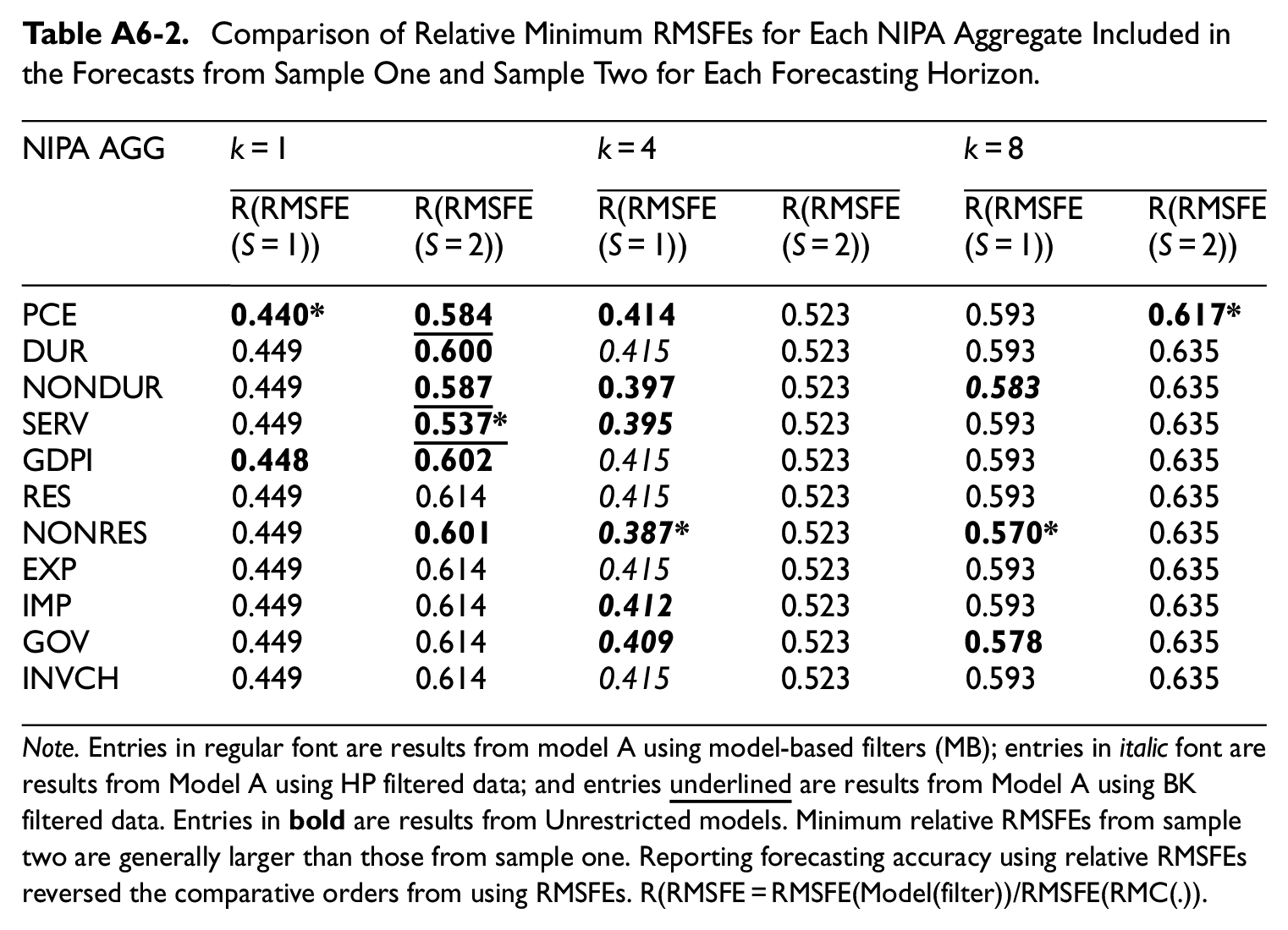
Having reported the results by sample and by forecasting horizon, it is useful to summarize the results across the forecasting horizons for each sample and between the two samples for each forecasting horizon. Thus far, we have evaluated forecasting accuracy relative to that of the benchmark model and have learned that using smoothed trend and cycle estimates rather than the unfiltered time series on real GDP produces more accurate forecasts. However, as the sizes of the RMSFEs from the benchmark model affect the sizes of the relative RMSFEs, if relative RMSFEs are used instead for comparison, the patterns of accuracy and patterns of relative accuracy across forecasting horizons from each sample or between the two samples for a given forecasting horizon may differ. Thus, we report the comparisons in terms of RMSFEs in the text and report the comparison in relative RMSFEs in Tables A6-1 to A6-2 in the Appendix.

Table 1 compares the minimum RMSFEs from the one-, four-, and eight-quarter ahead forecasts using data respectively from sample one and sample two. The last row in the Table displays the RMSFEs from the benchmark model for each forecasting horizon from each sample, the relative sizes of which indicate that the patterns of forecast accuracy measured in relative RMSFEs may differ from those measured in RMSFEs. Table 1 shows that the minimum RMSFEs from sample one forecasts monotonically increase as the forecasting horizon increases. However, the minimum RMSFEs from sample 2 forecasts increase only as forecasting horizon increases from four to eight quarters. When seven of the NIPA aggregates were included for the forecasts, the minimum RMSFEs from the one-quarter ahead forecasts are slightly larger than those from the four-quarter ahead forecasts.

Table 1.

Comparison of Minimum RMSFEs for Each NIPA Aggregate Included in the One-, Four-, and Eight-Step Ahead Forecasts Using Data from Sample One and Sample Two.

	Min(RMSFE) - Sample 1			Min(RMSFE) - Sample 2
NIPA AGG	RMSFE(k=1)	RMSFE(k=4)	RMSFE(k=8)	RMSFE(k=1)	RMSFE(k=4)	RMSFE(k=8)
PCE	0.0038*	0.0052	0.0053	0.0037	0.0038	0.0041*
DUR	0.0039	0.0052	0.0053	0.0038	0.0038	0.0042
NONDUR	0.0039	0.0049	0.0052	0.0037	0.0038	0.0042
SERV	0.0039	0.0049	0.0053	0.0034*	0.0038	0.0042
GDPI	0.0039	0.0052	0.0053	0.0038	0.0038	0.0042
RES	0.0039	0.0052	0.0053	0.0039	0.0038	0.0042
NONRES	0.0039	0.0048*	0.0050*	0.0038	0.0038	0.0042
EXP	0.0039	0.0052	0.0053	0.0039	0.0038	0.0042
IMP	0.0039	0.0051	0.0053	0.0039	0.0038	0.0042
GOV	0.0039	0.0051	0.0051	0.0039	0.0038	0.0042
INVCH	0.0039	0.0052	0.0053	0.0039	0.0038	0.0042
RMSFE(RMC)	0.0087	0.0125	0.0089	0.0064	0.0073	0.0066

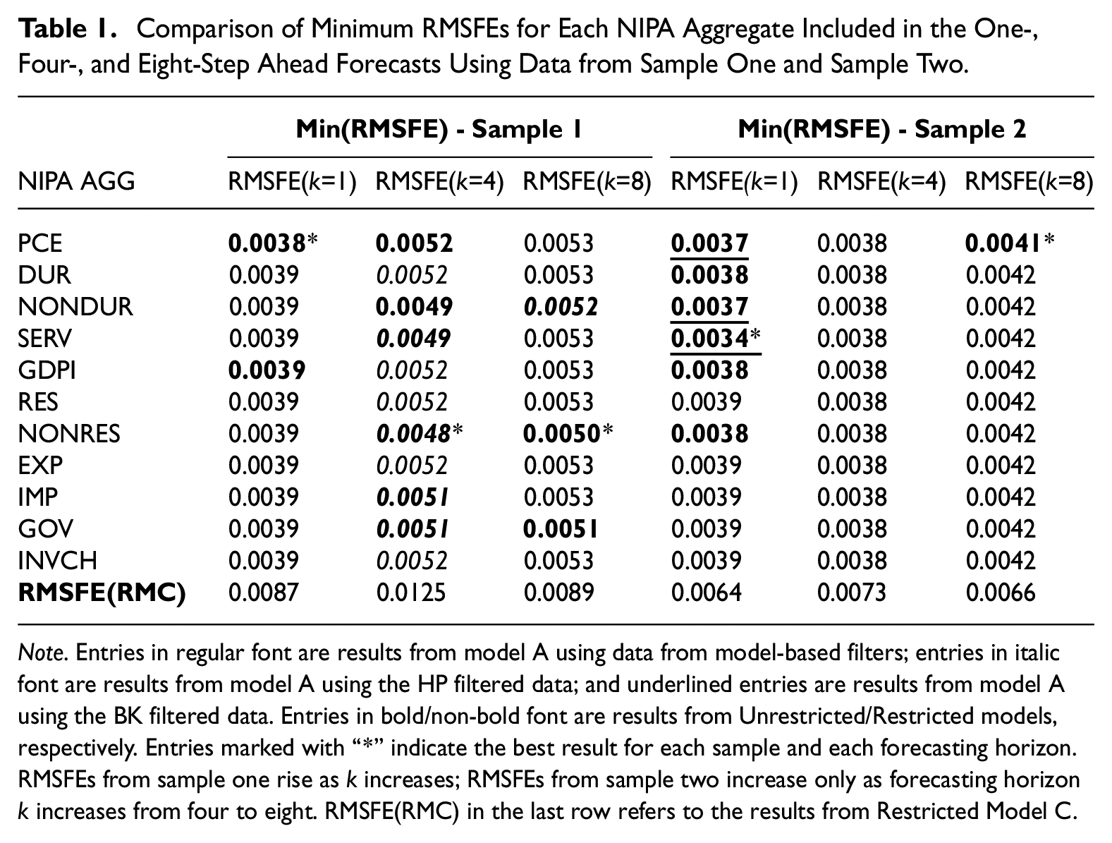
Note. Entries in regular font are results from model A using data from model-based filters; entries in italic font are results from model A using the HP filtered data; and underlined entries are results from model A using the BK filtered data. Entries in bold/non-bold font are results from Unrestricted/Restricted models, respectively. Entries marked with “*” indicate the best result for each sample and each forecasting horizon. RMSFEs from sample one rise as k increases; RMSFEs from sample two increase only as forecasting horizon k increases from four to eight. RMSFE(RMC) in the last row refers to the results from Restricted Model C.

Table 2 compares the results between the two samples. For each forecasting horizon, the minimum RMSFEs using data from sample one are larger than those using data from sample two. Such results seem to run counter to the expectation that larger forecasting errors are expected from the testing sample that covers the GR caused by the 2008 financial crisis. However, the second estimation sample is forty quarters longer than the first estimation sample. The additional observations may have provided more information, such that the forecasting models are able to a certain extent to capture what was happening during the GR.

Table 2.

Comparison of Minimum RMSFEs for Each NIPA Aggregate Included in the Forecasts from Sample One and Sample Two for Each Forecasting Horizon.

	k = 1		k = 4		k = 8
NIPA AGG	RMSFE(S=1)	RMSFE(S=2)	RMSFE(S=1)	RMSFE(S=2)	RMSFE(S=1)	RMSFE(S=2)
PCE	0.0038*	0.0037	0.0052	0.0038	0.0053	0.0041*
DUR	0.0039	0.0038	0.0052	0.0038	0.0053	0.0042
NONDUR	0.0039	0.0037	0.0049	0.0038	0.0052	0.0042
SERV	0.0039	0.0034*	0.0049	0.0038	0.0053	0.0042
GDPI	0.0039	0.0038	0.0052	0.0038	0.0053	0.0042
RES	0.0039	0.0039	0.0052	0.0038	0.0053	0.0042
NONRES	0.0039	0.0038	0.0048*	0.0038	0.0050*	0.0042
EXP	0.0039	0.0039	0.0052	0.0038	0.0053	0.0042
IMP	0.0039	0.0039	0.0051	0.0038	0.0053	0.0042
GOV	0.0039	0.0039	0.0051	0.0038	0.0051	0.0042
INVCH	0.0039	0.0039	0.0052	0.0038	0.0053	0.0042

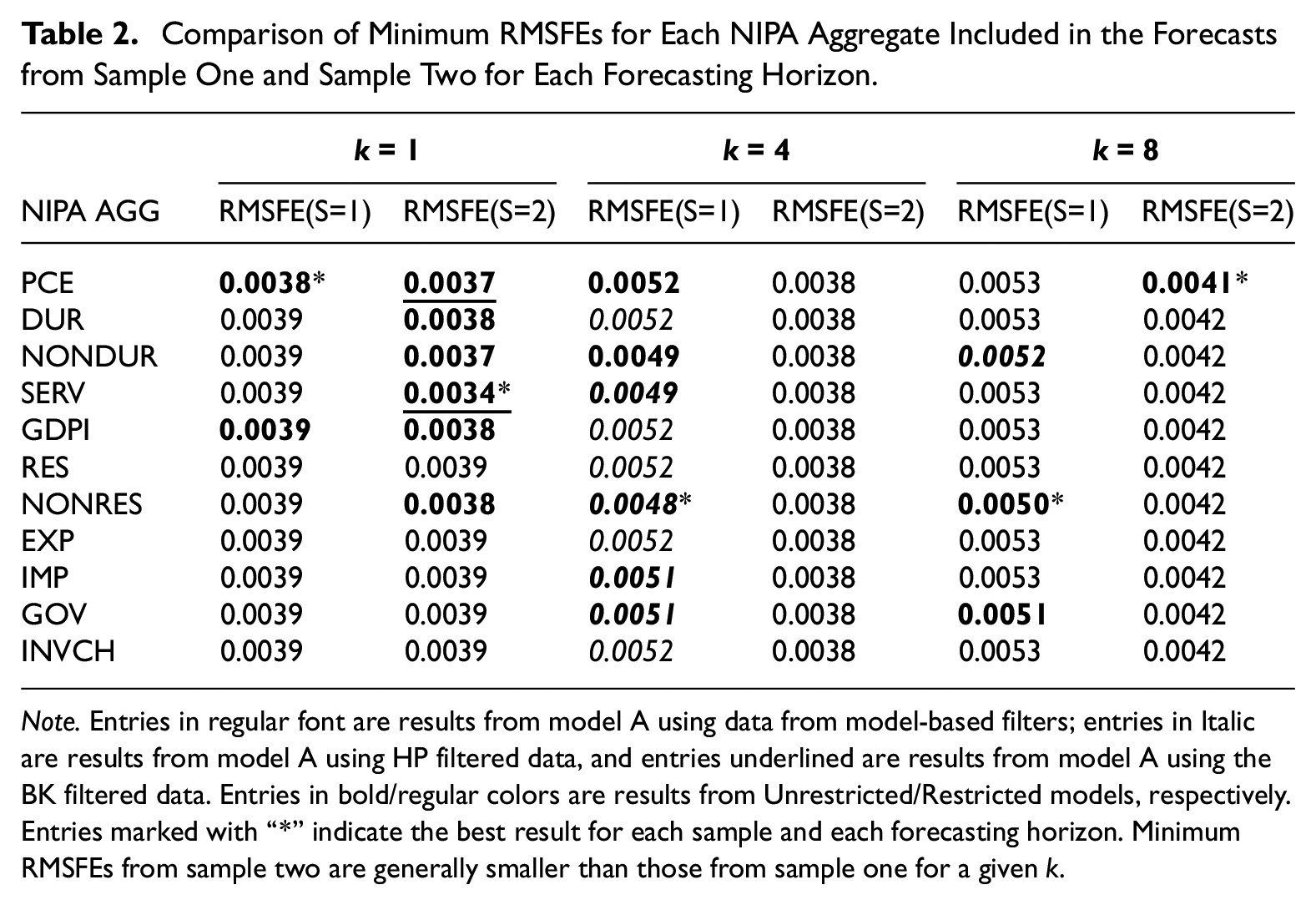
Note. Entries in regular font are results from model A using data from model-based filters; entries in Italic are results from model A using HP filtered data, and entries underlined are results from model A using the BK filtered data. Entries in bold/regular colors are results from Unrestricted/Restricted models, respectively. Entries marked with “*” indicate the best result for each sample and each forecasting horizon. Minimum RMSFEs from sample two are generally smaller than those from sample one for a given k.

At the outset of the forecasting exercises, we planned to investigate which model is the best for forecasting real GDP growth and which filtering technique is most desirable for that purpose. We also want to identify the NIPA aggregates, if any, that are capable of producing the best forecasts of real GDP growth.

Table 3 identifies total consumption, nonresidential investment, and consumption of services as the NIPA aggregates capable of producing the best forecasts of real GDP growth among five of the six scenarios. Table 3 also shows that model A is the best model for forecasting real GDP growth in all scenarios. Moreover, using the trend and cycle estimates from the selected BW and BAL filters produced the best forecasts in four of the six scenarios, among which three are from the unrestricted Model A. In the remaining two scenarios, the best forecasts are from unrestricted Model A using the trend and cycle estimates from the HP and BK filters. Note that column 5 in Table 3 displays the relative RMSFEs of the best forecast for each scenario, providing a comparison of the accuracy of the best forecast relative to that from the benchmark model.

Table 3.

The NIPA Aggregate, the Forecasting Model, and the Filtering Technique for Jointly Producing the Best Forecasts for Each Forecasting Horizon Using Data from Each Sample.

Sample/horizon	NIPA AGG	RMSFE	MODEL(FILTER)	R(RMSFE)	DM stat	p-Value (DM)
Sample 1, k = 1	PCE	3.83E-03	UMA(MB)	0.440	−2.93	.006
Sample 1, k = 4	NONRES	4.82E-03	UMA(HP)	0.387	−1.23	.224
Sample 1, k = 8	NONRES	5.04E-03	UMA(MB)	0.570	−1.37	.181
Sample 2, k = 1	SERV	3.42E-03	UMA(BK)	0.537	−4.30	.000
Sample 2, k = 4	**	3.82E-03	RMA(MB)	0.523	3.24	.003
Sample 2, k = 8	PCE	4.05E-03	UMA(MB)	0.617	−3.00	.005

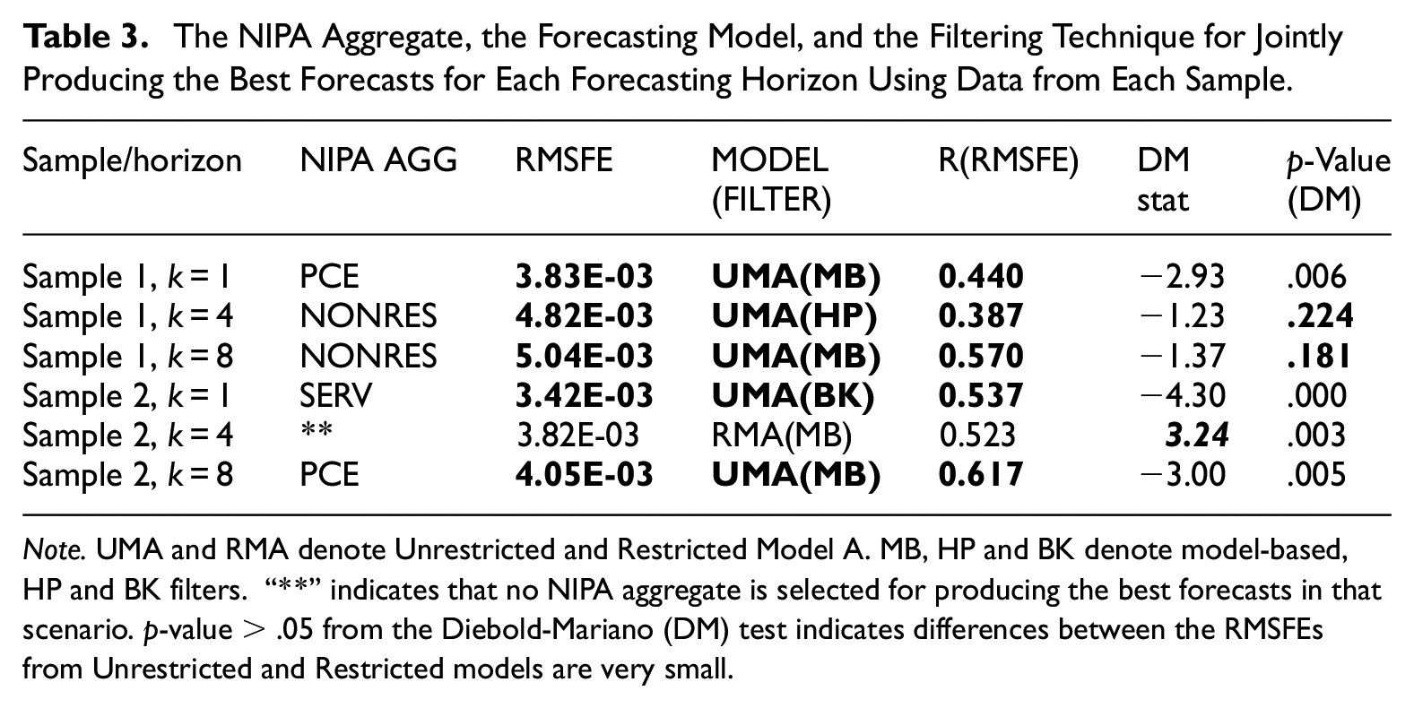
Note. UMA and RMA denote Unrestricted and Restricted Model A. MB, HP and BK denote model-based, HP and BK filters. “**” indicates that no NIPA aggregate is selected for producing the best forecasts in that scenario. p-value > .05 from the Diebold-Mariano (DM) test indicates differences between the RMSFEs from Unrestricted and Restricted models are very small.

The model-based BW and BAL filters are expected to have superior performances over the BK and the HP filters because the model-based filters adapted to the data. Although the HP and the BK filters have the advantage of being simple to calculate, our results have demonstrated stronger performances of the model-based BW and BAL filters for forecasting real GDP growth.

5. Discussion and Concluding Remarks

The study of business cycle fluctuations represents a foundation for applications such as current economic analysis, policymaking, and forecasting. This study has capitalized on the link between cyclical models and band-pass filters, which represents an area of ongoing development in econometrics and statistics. The core reason for applying a model-based BW and BAL filter is that the series has a cyclical component intertwined with other components, such as trend and noise, which must be effectively removed. In constructing an unobserved component model with such a cyclical process designed to generate periodic dynamics, the foundation is set for constructing filters that adapt to the different trend and other properties seen across diverse time series. Filter construction through model design gives a unified framework. Given the specifications of the components, a set of optimal filters arises.

This study has concentrated on a comprehensive and diverse dataset on the U.S. real GDP and eleven major NIPA aggregates and it has used the adaptive model-based BW and BAL filters to analyze and interpret properties and co-movements in business cycle components across series. The article provides a new set of empirical regularities via the examination of the lead-lag and Granger-causal relations between the aggregate cycles in real GDP and the cyclical movements in the NIPA aggregates, and via the investigation of the ability of the NIPA aggregates to forecast real GDP growth.

Patterns of cross-correlations computed from the cycles extracted with the BW and BAL filters are consistent with the observed lead-lag relationships between the aggregate cycles of real GDP and the cyclical movements of the NIPA aggregates. Granger-causality tests based on the cycles extracted with the BW and BAL filters confirmed empirically observed strong “feedback” causal relationships between real GDP and all consumption and investment aggregates as well as exports, and the test also confirmed the unidirectional causal relationship running from real GDP to imports. The “feedback” causal relationship between real GDP and government spending may seem contrary to Keynesian policies but may comport with other political realities.

Using data from two sample sets, the forecasting exercises have demonstrated the ability of some NIPA aggregates to forecast one-, four-, and eight-step ahead real GDP growth. The results favor the unrestricted two-step Model A that first separately forecasts the trend and cycle growth of real GDP allowing trend and cycle components of both real GDP and a NIPA aggregate to be included for the forecasts, and then combines the forecasted trend and cycle growth to obtain real GDP growth. Moreover, model-based BW and BAL filters outperformed the HP and BK filters. In four of the six scenarios, the best forecasts were produced from the trend and cycles extracted with the BW and BAL filters.

For comparison purposes, the HP and BK filters were also used for the analysis. The results based on the HP and BK filtered series are not always consistent with economic intuitions and empirical observations. The cross-correlations based on the HP and the BK filters are noticeably lower at the longer leads and longer lags than those based on the cycles extracted with the BW and BAL filters. Moreover, the HP filtered cycles revealed different lead-lag patterns between the aggregate cycles and the cyclical movements of some of the NIPA aggregates. Although a precise explanation for these differing correlation patterns is yet to be explored, the much noisier cycles extracted with the HP filter perhaps could offer an explanation.

Granger-causality tests based on the BK filtered cycles concluded unidirectional causal relations running from real GDP to the consumption of durables and nondurables, as well as the unidirectional causal relations running from total consumption and consumption of services to real GDP. Granger tests based on the HP-filtered cycles concluded the unidirectional causal relations running from real GDP to real investment and a “feedback” causal relation between real GDP and imports, which run counter to the empirical observations and economic intuitions.

In the forecasting exercises, the HP filtered trend and cycle produced best four-quarter ahead forecasts in the unrestricted two-step Model A using data from sample one, but BK filtered trend and cycle series did not produce the best forecasts in any of the six scenarios.

The basic conclusion from the empirical analysis is that the adaptive model-based BW and BAL filters have demonstrated the advantages over the commonly used HP and BK filters for analyzing and interpreting the properties and co-movements in business cycle components across very diverse economic series from the U.S. national accounts. This is because these filters are implicitly defined by the models, which in turn are adapted to the data.

Supplemental Material

sj-docx-1-jof-10.1177_0282423X241263763 – Supplemental material for Cycle Fluctuations in the U.S. Real GDP and National Income and Product Accounts Aggregates

Supplemental material, sj-docx-1-jof-10.1177_0282423X241263763 for Cycle Fluctuations in the U.S. Real GDP and National Income and Product Accounts Aggregates by Baoline Chen, Kyle Hood, Tucker McElroy and Thomas Trimbur in Journal of Official Statistics

Footnotes

Appendix

Table A6-2.

Comparison of Relative Minimum RMSFEs for Each NIPA Aggregate Included in the Forecasts from Sample One and Sample Two for Each Forecasting Horizon.

NIPA AGG	k = 1		k = 4		k = 8
NIPA AGG	R(RMSFE(S = 1))	R(RMSFE(S = 2))	R(RMSFE(S = 1))	R(RMSFE(S = 2))	R(RMSFE(S = 1))	R(RMSFE(S = 2))
PCE	0.440*	0.584	0.414	0.523	0.593	0.617*
DUR	0.449	0.600	0.415	0.523	0.593	0.635
NONDUR	0.449	0.587	0.397	0.523	0.583	0.635
SERV	0.449	0.537*	0.395	0.523	0.593	0.635
GDPI	0.448	0.602	0.415	0.523	0.593	0.635
RES	0.449	0.614	0.415	0.523	0.593	0.635
NONRES	0.449	0.601	0.387*	0.523	0.570*	0.635
EXP	0.449	0.614	0.415	0.523	0.593	0.635
IMP	0.449	0.614	0.412	0.523	0.593	0.635
GOV	0.449	0.614	0.409	0.523	0.578	0.635
INVCH	0.449	0.614	0.415	0.523	0.593	0.635

Note. Entries in regular font are results from model A using model-based filters (MB); entries in italic font are results from Model A using HP filtered data; and entries underlined are results from Model A using BK filtered data. Entries in bold are results from Unrestricted models. Minimum relative RMSFEs from sample two are generally larger than those from sample one. Reporting forecasting accuracy using relative RMSFEs reversed the comparative orders from using RMSFEs. R(RMSFE = RMSFE(Model(filter))/RMSFE(RMC(.)).

Acknowledgements

We appreciate five anonymous referees and an Associate Editor for their helpful comments and suggestions which have helped improve our paper. We also appreciate the audiences at the 2022 Joint Statistical Meetings (JSM), Washington, DC, U.S. and the 2023 Society for Economic Measurement (SEM) conference, Milan, Italy for their helpful comments.

Funding

The author(s) received no financial support for the research, authorship, and/or publication of this article.

Disclaimer

This paper reflects the views of the authors and does not represent the official opinions of the U.S. Bureau of Economic Analysis and the U.S. Census Bureau.

ORCID iD

Baoline Chen

Supplemental Material

Supplemental material for this article is available online.

References

Akaike

1976. “Canonical Correlation Analysis of Time Series and the Use of an Information Criterion.”Mathematics in Science and Engineering 126: 27–96. DOI: https://doi.org/10.1016/S0076-5392(08)60869-3.

Baxter

King

R. G.

1999. “Measuring Business Cycles: Approximate Band-Pass Filters for Economic Time Series.”Review of Economics and Statistics 81: 575–93. DOI: https://doi.org/10.1162/003465399558454.

Bell

W. R.

1984. “Signal Extraction for Nonstationary Time Series.”Annals of Statistics 12: 646–64. DOI: https://doi.org/10.1214/aos/1176346512.

Buss

2010. “Asymmetric Baxter-King Filter.”Technologies of Computer Control 42: 95–9.

Butterworth

1930. “On the Theory of Filter Amplifiers.”Experimental Wireless & the Wireless Engineer7: 536–41.

Canova

2020. “FAQ: How Do I Measure the Output Gap?” CEPR Discussion Papers 14943.

Celov

Comunale

2023. “Business Cycles in the EU: A Comprehensive Comparison Across Methods.” In Essays in Honor of Fabio Canova, edited by J. J.

Dolado

Gambetti

Matthes

, 99–146. Bingley: Emerald Publishing Limited. DOI: https://doi.org/10.1108/s0731-90532022000044b004.

Fisher

J. D. M.

2007. “Why Does Household Investment Lead Business Investment Over the Business Cycle?”Journal of Political Economy 115 (1): 141–68. DOI: https://doi.org/10.1086/511994.

Gómez

2001. “The Use of Butterworth Filters for Trend and Cycle Estimation in Economic Time Series.”Journal of Business & Economic Statistics 19: 365–73. DOI: https://doi.org/10.1198/073500101681019909.

10.

Granger

C. W. J.

1969. “Investigating Causal Relations by Econometric Models and Cross-Spectral Methods.”Econometrica 37 (3): 424–38. DOI: https://doi.org/10.2307/1912791.

11.

Green

R. K.

1997. “Follow the Leader: How Changes in Residential and Non-Residential Investment Predict Changes in GDP.”Real Estate Economics 25 (2): 253–70. DOI: https://doi.org/10.1111/1540-6229.00714.

12.

Guan

J. L.

Hong

2012. “An Empirical Analysis on U.S. Foreign Trade and Economic Growth.”AASRI Procedia 2: 39–43. DOI: https://doi.org/10.1016/j.aasri.2012.09.011.

13.

Hamilton

J. D.

2018. “Why You Should Never Use the Hodrick-Prescott Filter.”Review of Economics and Statistics 100 (5): 831–43. DOI: https://doi.org/10.1162/rest_a_00706.

14.

Harvey

A. C.

Trimbur

2003. “General Model-Based Filters for Extracting Cycles and Trends in Economic Time Series.”Review of Economics and Statistics 85: 244–55. DOI: https://doi.org/10.1162/003465303765299774.

15.

Hodrick

R. J.

Prescott

E. C.

1997. “Postwar US Business Cycles: An Empirical Investigation.”Journal of Money, Credit and Banking 24: 1–16. DOI: https://doi.org/10.2307/2953682.

16.

Kamal

Ouyang

Handley

2022. “The Rise of Exporters and Importers in US Job Growth: Insights from Newly Released Data.” The Center for Economic Policy Research (CEPR), VoxEU Column, February14.

17.

Kliesen

2016. “Are Key Investment Indicators Signaling a Recession?”On the Economy Blog, Federal Reserve Bank of St. Louis Office, August4.

18.

McElroy

2008. “Exact Formulas for the Hodrick-Prescott Filter.”The Econometrics Journal 11 (1): 209–17. DOI: https://doi.org/10.1111/j.1368-423x.2008.00230.x.

19.

Mohr

2005. “A Trend-Cycle (-Season) Filter.” Working Paper No. 499, European Central Bank, 1–46. DOI: https://doi.org/10.2139/ssrn.726694.

20.

Nyasha

Odhiambo

N. M.

2019. “Government Size and Economic Growth: A Review of International Literature.”SAGE Open 9: 2158244019877200. DOI: https://doi.org/10.1177/2158244019877.

21.

Ortiz-Ospina

Beltekian

Roser

2018. “The Concept Link Between Trade and Household Welfare.”Trade and Globalization.

22.

Pollock

D. S. G.

2016. “Econometric Filters.”Computational Economics 48 (4): 669–91. DOI: https://doi.org/10.1007/s10614-015-9543-2.

23.

Stock

J. H.

Watson

M. W.

1999. “Business Cycle Fluctuations in US Macroeconomic Time Series.”Handbook of Macroeconomics 1: 3–64. DOI: https://doi.org/10.1016/s1574-0048(99)01004-6.

24.

Trimbur

T. M.

2006. “Properties of Higher Order Stochastic Cycles.”Journal of Time Series Analysis 27: 1–17. DOI: https://doi.org/10.1111/j.0143-9782.2005.00462.x.

25.

Trimbur

T. M.

McElroy

T. S.

2022. “Modelled Approximations to the Ideal Filter with Application to Time Series of Gross Domestic Product.”The Annals of Applied Statistics 16 (2): 627–51. DOI: https://doi.org/10.1214/21-aoas1463.

26.

U.S. Bureau of Economic Analysis. 2018. “National Accounts Data.”https://apps.bea.gov/iTable (accessed November 30, 2018).

27.

Zestos

G. K.

Tao

2002. “Trade and GDP Growth: Causal Relations in the United States and Canada.”Southern Economic Journal 68 (4): 859–74. DOI: https://doi.org/10.2307/1061496.

Supplementary Material

Please find the following supplemental material available below.

For Open Access articles published under a Creative Commons License, all supplemental material carries the same license as the article it is associated with.

For non-Open Access articles published, all supplemental material carries a non-exclusive license, and permission requests for re-use of supplemental material or any part of supplemental material shall be sent directly to the copyright owner as specified in the copyright notice associated with the article.

0.00 MB

1.24 MB