
Abstract
In small area estimation, it is sometimes necessary to use model-based methods to produce estimates in areas with little or no data. In official statistics, we often require that aggregates of small area estimates agree with national estimates for internal consistency purposes. Enforcing this agreement is referred to as benchmarking, and while methods currently exist to perform benchmarking, few are ideal for applications with non-normal outcomes and benchmarks with uncertainty. Fully Bayesian benchmarking is a theoretically appealing approach insofar as we can obtain posterior distributions conditional on a benchmarking constraint. However, existing implementations may be computationally prohibitive. In this paper, we critically review benchmarking methods in the context of small area estimation in low- and middle-income countries with binary outcomes and uncertain benchmarks, and propose a novel approach in which posterior samples of small area characteristics from an unbenchmarked model can be combined with a rejection sampler or Metropolis-Hastings algorithm to produce benchmarked posterior distributions in a computationally efficient way. To illustrate the flexibility and efficiency of our approach, we provide comparisons to an existing benchmarking approach in a simulation, and applications to HIV prevalence and under-5 mortality estimation. Code implementing our methodology is available in the R package stbench.
1. Introduction
In a public health context, small area estimates, where small areas are defined as domains with little to no data, are often produced by official statistics agencies for the purpose of informing targeted public health interventions. In low-and middle-income countries (LMICs), the most reliable source of public health information is household surveys such as Demographic and Health Surveys (DHS) and Multiple Indicator Cluster Surveys (MICS), and as such, direct (weighted) survey estimates are considered the gold standard when they are precise enough to be practically useful. In small area estimation, where we have by definition little to no data in certain domains, it may not be possible to obtain direct, survey estimates with reasonable precision. In these settings, model-based methods are often used when estimates at small levels of aggregation are required (Rao and Molina 2015). Model-based methods that incorporate spatial random effects, in the absence of reliable covariate information, allow for estimates in all small areas to be produced with little to no data, introducing some bias into the estimates in exchange for tighter interval estimates (Knorr-Held 2000; Riebler et al. 2016; Wakefield et al. 2020). Area-level models, such as the popular Fay-Herriot model (Fay and Herriot 1979), consider data at the level of the small area, whereas unit-level models consider data at the level of the individual or cluster (Battese et al. 1988). When area-level sample sizes are particularly small, unit-level models may be more desirable. For a review of both area-level and unit-level models, see Chapters 4 to 7 of Rao and Molina (2015).
It is often required that small area estimates agree with estimates at a higher level of aggregation. For example, subnational estimates may be required to aggregate to a national estimate. These higher level estimates are referred to as benchmarks, and are frequently considered more reliable than small area estimates since more data are available to inform them, or they are direct (weighted) estimates and therefore less dependent on model assumptions. Note that benchmarking as we consider it in this paper is distinct from calibration weighting (Särndal et al. 2003; Si and Zhou 2020). The latter involves incorporating known, population-level covariate information into a model to adjust for potential bias in a subnational model, while the former involves incorporating known, population-level outcome information into a model to enforce internal consistency in an official statistics setting.
Benchmarks may be from the same data source that was used to produce small area estimates or from an outside source, referred to as internal benchmarking and external benchmarking, respectively (Bell et al. 2013). In an internal benchmarking setting, the use of the same data twice—once to calculate model-based small area estimates and also to define benchmarks at a higher level of spatial aggregation—may lead to an understating of statistical uncertainty unless additional care is taken. The method of You et al. (2002) can be used to quantify the posterior mean squared error (MSE) of an internally benchmarked predictor in a Bayesian context. We also direct the reader to Pfeffermann and Tiller (2006) for an approach to assessing the uncertainty of internally benchmarked predictors. We note that the particular applications we consider in this paper are in an external benchmarking setting, and that this setting is relatively common in global health applications (Eaton et al. 2021; Osgood-Zimmerman et al. 2018) as well as more recent applications in agriculture (Chen et al. 2022). Internal benchmarking settings and their limitations are outside the scope of this paper.
Many existing benchmarking approaches treat benchmarking as a constraint problem, where estimates at smaller areas are constrained to agree with estimates at a higher level of aggregation. Approaches vary by the ways in which constraints have been incorporated into a modeling framework, and as such, the interpretation of resulting benchmarked estimates varies by approach. There are many ways to categorize benchmarking approaches, but one we may consider is a one-step versus two-step procedure. In a two-step procedure, estimates and uncertainty are first obtained from a model that is agnostic to the benchmarking constraint and are then adjusted to satisfy the benchmarking constraint. Datta et al. (2011), Ghosh and Steorts (2013), Steorts et al. (2020), Wang et al. (2008), Patra and Dunson (2018), Patra (2019), Ghosh et al. (2015), and Williams and Berg (2013) and Berg and Fuller (2018) all consider a two-step procedure where benchmarked estimates are calculated by minimizing posterior expected loss (for a given loss function) subject to a benchmarking constraint. Unbenchmarked estimates are first obtained, and then projected into a constrained space.
Other two-step procedures include difference benchmarking and ratio benchmarking (henceforth referred to as raking), described in Erciulescu et al. (2019). Again, a model that is agnostic to the benchmarking constraint is first fit, and then estimates are adjusted by a constant so that the benchmarking constraint is satisfied (Erciulescu et al. 2018, 2019, 2020). You et al. (2002) consider a hierarchical Bayesian model for unbenchmarked estimates, but obtain benchmarked estimates using the raking method, and quantify uncertainty via posterior MSE as opposed to estimating full posterior distributions for benchmarked estimates.
Other benchmarking approaches incorporate the benchmarking constraint into the data likelihood—referred to as an augmented model in Bell et al. (2013), Berg and Fuller (2018), and Stefan and Hidiroglou (2021)—and thus produce automatically benchmarked estimates in a single modeling step. You and Rao (2002) also follow this approach, and refer to this as a “self-benchmarking” property. Others (Erciulescu et al. 2019; Janicki and Vesper 2017; Nandram et al. 2019; Nandram and Sayit 2011; Zhang and Bryant 2020) propose benchmarking approaches that produce full, benchmarked posterior distributions for small area estimates, making uncertainty quantification straightforward in an external benchmarking setting. Following Zhang and Bryant (2020), we refer to such approaches as fully Bayesian benchmarking approaches. Note that we consider this type of approach to be distinct from fitting a Bayesian model and benchmarking only point estimates. Nandram and Sayit (2011) develop a fully Bayesian benchmarking approach specifically for betabinomial models. Janicki and Vesper (2017) perform fully Bayesian benchmarking by minimizing the KL divergence between a benchmarked and unbenchmarked posterior using moment constraints. Nandram et al. (2019) perform fully Bayesian benchmarking using a transformation of the benchmarking constraint that corresponds to “deleting” a single small area, but note that benchmarked estimates vary based on which area is deleted. Erciulescu et al. (2019) consider four different benchmarking approaches, one of which is the Bayesian method described in Nandram and Sayit (2011), and three of which involve fitting a hierarchical Bayesian model and benchmarking point estimates using ratio or difference benchmarking. Zhang and Bryant (2020) develop a fully Bayesian benchmarking approach that produces full posterior distributions conditional on either a soft or hard benchmarking constraint.
Benchmarking approaches have also been developed in a time series context, with certain similarities to small area estimation in requiring finer estimates in time to agree with aggregate estimates across multiple years (Dagum and Cholette 2006). Different benchmarking approaches are more or less appealing than others—depending on context—with regards to obtaining measures of uncertainty, computational tractability, and the way in which the benchmarking constraint is enforced.
Benchmarking methods may also differ depending on whether benchmarking must be exact or inexact. In exact benchmarking, as the name suggests, the benchmarking constraint must hold exactly, whereas in inexact benchmarking the constraint must hold within some margin of error. The latter can be viewed as a soft constraint as opposed to a hard constraint. Exact benchmarking may be appropriate if the benchmarks are unbiased and have little to no uncertainty, which can occur when they come from a census (Trabelsi and Hillmer 1990). Inexact, external benchmarking may be appropriate if national estimates come from a different survey and contain appreciable sampling error, as discussed in Hillmer and Trabelsi (1987), or if national estimates are model-based with appreciable uncertainty, as in the settings we consider in our application.
In this article, we present two novel implementations of the fully Bayesian benchmarking approach described in Zhang and Bryant (2020) that are more flexible and computationally tractable in many settings. Our approaches combine an unbenchmarked model with either a rejection sampler or Metropolis-Hastings algorithm to produce fully Bayesian benchmarked posteriors, which we describe in Subsection 3.4. We compare our method to that described in Zhang and Bryant (2020) in the setting of modeling HIV prevalence in South Africa, as well as modeling under-5 mortality rates (U5MR) in Namibia. These applications were chosen to demonstrate the flexibility of the proposed fully Bayesian approaches in estimating outcomes that lie between 0 and 1 with unique benchmarking constraints, the efficiency of the method in cases where the benchmarks are very consistent or inconsistent with the small area estimates, and the flexibility of the approaches to handle both area-level and unit-level models. To emphasize the novelty of our approaches and computational advantages of the proposed method over the Markov chain Monte Carlo (MCMC) samplers used in Zhang and Bryant (2020) in terms of flexibility, we use integrated nested Laplace approximation (INLA) and Template Model Builder (TMB) as alternative ways to conduct Bayesian inference using Laplace approximations, that are fast and do not require users to code model-specific fitting routines (Kristensen et al. 2016; Rue et al. 2009). We additionally compare run times for our proposed approaches to that of Zhang and Bryant (2020) in a simulation, and show that our proposed approaches provide not only increased flexibility in terms of modeling for Bayesian inference, but computational speed gains as well. All code for fitting the models described in this paper is available via the R package stbench, found at https://github.com/taylorokonek/stbench.
2. Small Area Models in Low- and Middle-Income Countries
The estimation of U5MR in LMICs at a subnational level motivates our desire for benchmarking. The UN Inter-agency Group for Child Mortality Estimation (IGME) produces annual, national level estimates of U5MR for all countries using a Bayesian B-spline bias-reduction (B3) method (Alkema and New 2014). Various data are used to produce B3 estimates, including vital registration, census, and household surveys, and many of these sources cannot be used for producing subnational estimates because geographic information is lacking, or the data type is not amenable to incorporate into a small area model. Subnational estimates of U5MR are of interest in addition to national estimates, in accordance with the Sustainable Development Goals (https://sustainabledevelopment.un.org/post2015/transformingourworld).
Model-based small area estimation has a long history in LMICs. While small area estimates that incorporate the survey design directly are preferred, they are often impractical at a small area level, with either too little precision to be practically useful or no data available in some small areas (Lehtonen and Veijanen 2009; Wakefield et al. 2020). This lack of data primarily comes from a disconnect between the administrative level at which these surveys are designed to produce reliable estimates (often administrative level 1, or state) and the administrative level at which public health interventions are made (often administrative level 2, or county). Model-based methods with spatial smoothing terms allow us to obtain precise estimates in all small areas, as required for public health estimates (Datta 2009; Wakefield et al. 2020).
Due to these smoothing terms and the inability to use data sources without geographic information to produce small area estimates, benchmarking is required to align subnational estimates with national estimates from the B3 model for internal consistency within the production of UN IGME estimates. Subnational estimates are currently produced for a handful of countries using a Beta-binomial model described in Wu et al. (2021), but benchmarking approaches in this context have not yet been rigorously explored. As national estimates are model-based (with uncertainty) in this context, we aim to use a benchmarking approach that incorporates national level uncertainty (i.e., is inexact).
Many public health outcomes, including HIV prevalence and U5MR that we consider for our applications, are estimated from Bernoulli or binomial counts. As such, binomial models are a typical choice in an LMIC setting (Eaton et al. 2021; Wu et al. 2021). We aim to use a benchmarking approach that is well-suited to binomial models with estimates that are proportions, and hence lie between 0 and 1. Just as the unbenchmarked estimates will lie in this range, the benchmarked estimates from our chosen benchmarking approach should as well.
Additionally, the approach we use should be fast and computationally flexible. These properties are particularly important in an LMIC setting, as practitioners and national statistics offices in LMICs may not have the same computational resources as those in high-income countries.
While our motivation for benchmarking primarily comes from subnational estimation of U5MR, the application to HIV prevalence is similarly important in a LMIC context, in that small area estimates of HIV prevalence are produced in an official statistics setting by UNAIDS and require benchmarking for internal consistency (Eaton et al. 2021). Similarly to U5MR, subnational estimates of HIV prevalence inform public health interventions and allow countries to monitor their progress toward the Sustainable Development Goals. The theoretical properties, computational speed, and flexibility of our proposed approaches are relevant to HIV prevalence estimation in LMICs, as (similarly to U5MR) national estimates are produced with uncertainty, and benchmarked estimates should lie between 0 and 1.
2.1. Small Area Models
Below we describe the unbenchmarked models that we consider for the HIV application, but they are generally appropriate for a binary outcome. The unbenchmarked models for the U5MR application are described in Subsection 2.2 of the Supplemental data. If there are sufficient data in each target area, then weighted (direct) estimates are reliable. Such estimates include the Horvitz-Thompson (HT) (Horvitz and Thompson 1952) and Hájek estimators (Hájek 1971). In situations where the direct estimates can be calculated but have unacceptably high design variance, one may smooth using an area-level model, such as the model of Fay and Herriot (1979). When the data are sparser still, area-level direct estimates may be unusable. With very little data, the variance estimate can be statistically unreliable or may not be calculable at all. In these cases, the raw data (counts, in the binary context) are modeled (in our HIV and U5MR examples, at the cluster level) to give a unit-level model.
2.1.1. Area-Level Model: Spatial Fay-Herriot
Let the HT estimator for area i be denoted
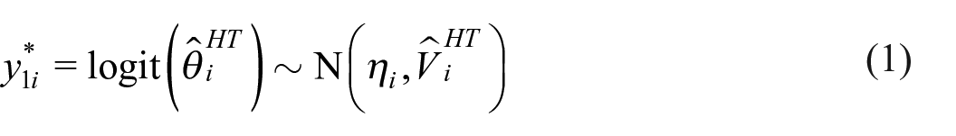
where

where
For priors, we set
2.1.2. Unit-Level Model: Binomial
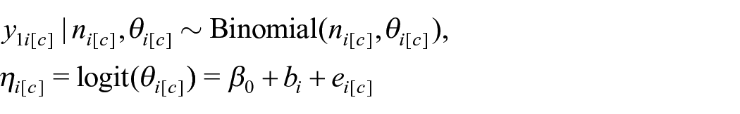
We may assume binomial observations of the outcome for each cluster c within area i. Let
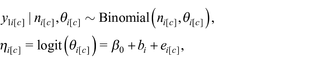
where
Area-level predictions
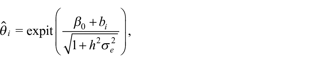
where
3. Methods
Let
Throughout the paper, we consider benchmarking constraints of the most basic form,
In the following subsections we describe a subset of existing approaches to benchmarking and propose two novel approaches to fully Bayesian benchmarking. The methods we describe in detail were chosen either because they are commonly used benchmarking methods in an official statistics setting, or because they are particularly relevant to our motivating application. One method is not inherently preferable, though we argue that some are more appropriate than others in the context of estimating outcomes between 0 and 1 in LMICs. The only existing fully Bayesian approach we describe is that of Zhang and Bryant (2020), as our proposed approach builds directly from their methodology.
3.1. Benchmarked Bayes Estimate Approach
The first approach we describe was developed in a Bayesian, decision theoretic framework (Datta et al. 2011; Steorts et al. 2020). This involves minimizing expected posterior MSE loss subject to the benchmarking constraint, which results in a projection of the unbenchmarked estimates into a benchmarked (constrained) space. Since its development, others have extended this decision theoretic approach with different loss functions (Berg and Fuller 2018; Ghosh et al. 2015; Williams and Berg 2013). Methods have also recently been developed to obtain benchmarked uncertainty for these estimates under this decision theoretic framework (Patra 2019; Patra and Dunson 2018). As it involves minimizing expected posterior loss subject to a benchmarking constraint we call this approach the Benchmarked Bayes Estimate approach. Though we will argue that this approach is not appropriate for our motivating application, we detail it here as it is theoretically appealing, fast, and commonly used in many benchmarking applications.
For n small areas, let
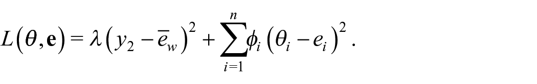
As Datta et al. (2011) are interested in an estimate of the benchmarked posterior mean, they consider minimizing the posterior expectation of the weighted squared error loss
where
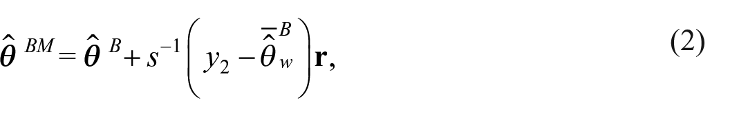
To obtain uncertainty around the benchmarked estimates, posterior samples can be projected into the space defined by the benchmarking constraint (Patra 2019; Patra and Dunson 2018). Geometrically, we can interpret this benchmarked Bayes estimate as the point estimate within the space defined by the benchmarking constraint that is as close to the unbenchmarked Bayes estimate as possible, where closeness is measured in terms of expected weighted squared error (Steorts et al. 2020).
The benchmarked estimate from Equation (2) is an exactly benchmarked estimate, that is, the benchmarking constraint holds exactly. Alternatively, in inexact benchmarking, the benchmarking constraint need not hold exactly. If inexact benchmarking is desired in the benchmarked Bayes estimate framework, a penalty term
The Bayes estimate associated with this loss is
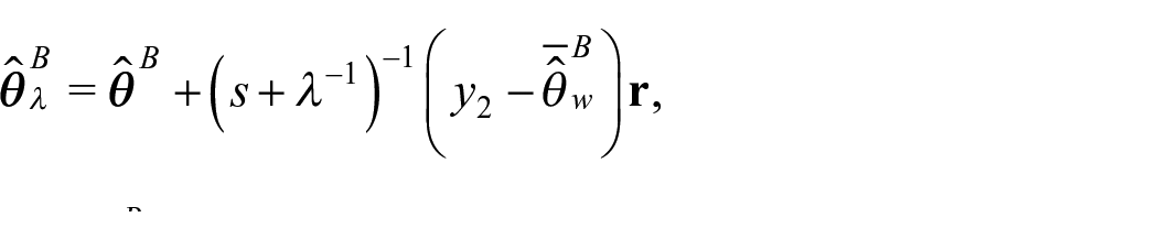
where we note that as
In the context of U5MR and HIV prevalence, the outcome of interest lies between 0 and 1, and may be close to 0. Any estimate that falls outside of
The benchmarked Bayes estimate approach is fast and theoretically justified in settings where estimates fall on the real line, are positive as in Ghosh et al. (2015), or lie well within the boundary of
3.2. Raking Approach
The second benchmarking approach we consider is simple and popular: raking, also referred to as the ratio-adjustment method (Datta et al. 2011; Ghosh et al. 2015; Zhang and Bryant 2020). A version of the raking approach is used by the Institute for Health Metrics and Evaluation (IHME) in a variety of applications (e.g., Osgood-Zimmerman et al. (2018) and Local Burden of Disease HIV Collaborators (2021)), in the Naomi model for estimating HIV prevalence and incidence (Eaton et al. 2021), and in the subnational U5MR estimates currently produced by UN IGME (Wu et al. 2021). This approach is commonly applied post hoc. The key feature of the raking approach is a ratio comparing an unbenchmarked national estimate to the national level benchmark
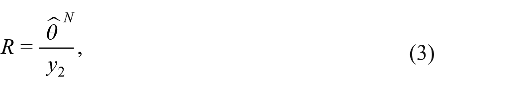
where
In a post hoc raking approach and with a sampling-based method, the posterior draws of
The raking approach to benchmarking can also be approximated via the inclusion of a log offset term for the ratio comparing an unbenchmarked national estimate to the national level benchmark in logistic models when the outcome of interest is rare, as in under-5 mortality estimation. In the supplement of Wakefield et al. (2019) they show that, for rare outcomes, including a log offset for R in a logistic regression model corresponds approximately to the same multiplicative bias adjustment that would be done in the post hoc raking approach. This approach is currently used in the UN IGME’s subnational U5MR estimates. We note that the form of raking involving the inclusion of a log offset for R does in fact produce fully Bayesian estimates, in the sense that a full posterior distribution for the benchmarked estimates is produced. However, the approach differs from the fully Bayesian approach described in Section 3.3 in that a likelihood is not specified for the benchmarks themselves.
3.3. Fully Bayesian Benchmarking Approach
Consider an area-level, Bayesian hierarchical model for small area estimation (Zhang and Bryant 2020). For n small areas, let the area-level parameters we wish to estimate be denoted by

Though Zhang and Bryant (2020) consider more complex forms of benchmarking constraints, for simplicity we again consider the constraint
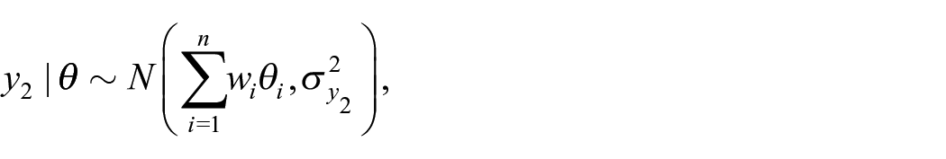
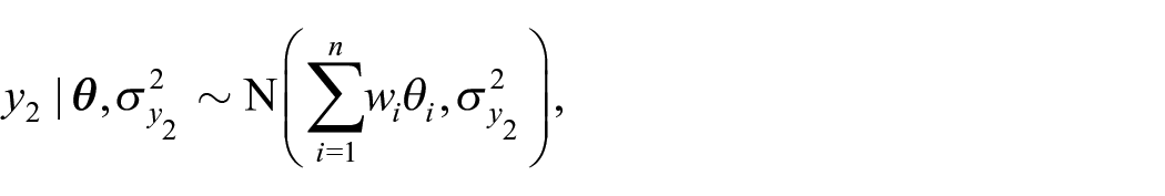
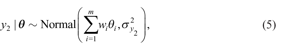
To incorporate the benchmarking constraint into their hierarchical model, Zhang and Bryant (2020) define an additional likelihood term for the benchmarks,

with the assumptions that
Under exact benchmarking, we set
A benefit of this benchmarking approach is that it allows for nonlinear benchmarking constraints. This is particularly relevant for logistic models, where the benchmarking constraint may take the form
The fully Bayesian benchmarking approach can be used with both area-level and unit-level models. Though Zhang and Bryant (2020) describe an extension of their fully Bayesian approach to unit-level models, an implementation of this does not currently exist. Zhang and Bryant (2020) provide code in their R package demest for Poisson, binomial, multinomial, and normal models, with optional point mass, Poisson, binomial, and normal distributions for the likelihood for the benchmark, found at https://github.com/StatisticsNZ/demest. They provide an outline for a MCMC scheme for a general model. However, implementation of this MCMC scheme will be model-specific, which can limit the uptake of the method. Statistical programs such as INLA and TMB provide alternative ways to conduct Bayesian inference which have great computational advantages over MCMC samplers. These computational advantages are described in detail for INLA in Rue et al. (2009) and for TMB in Kristensen et al. (2016), and involve the use of Laplace approximations to obtain posterior distributions at a fraction of the time it would take using MCMC algorithms. The methods are particularly suited to space and space-time modeling with Markov random field models—situations in which MCMC can be especially computationally demanding because of the dependence in the posterior (Margossian et al. 2020).
The benchmarking approach we propose in the following section is a more general implementation of the inexact, fully Bayesian approach described by Zhang and Bryant (2020), and allows us to obtain fully Bayesian benchmarked estimates from any method that produces area-level samples from an unbenchmarked model. The approach we propose is readily applicable to both area- and unit-level models, so long as area-level samples can be produced, and can be used in conjunction with statistical programs such as INLA and TMB.
3.4. Proposed Approach
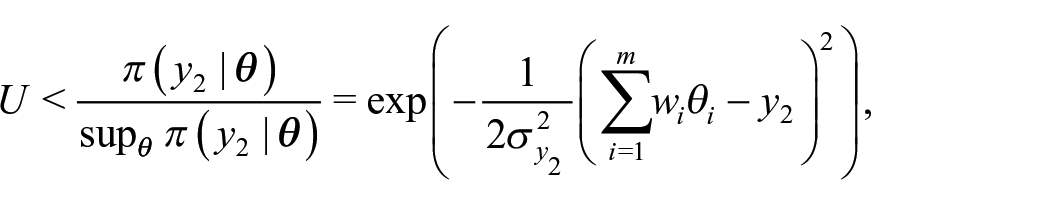
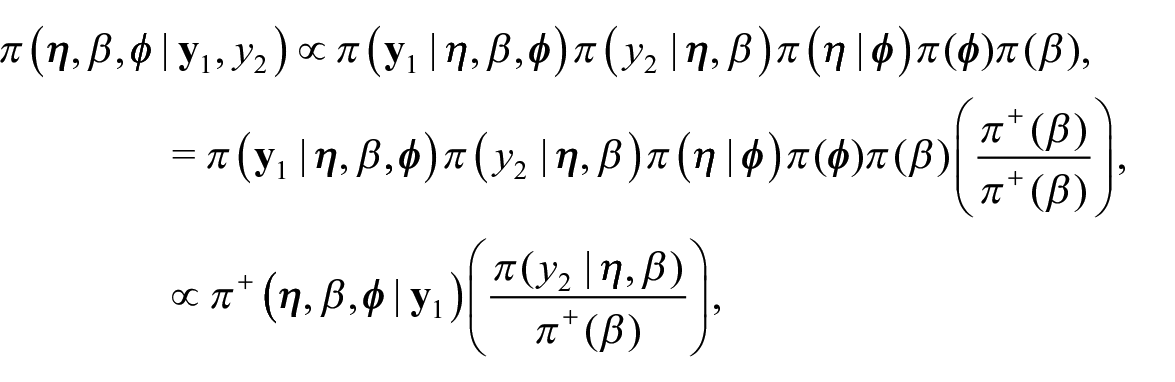
We propose an external benchmarking approach that combines an unbenchmarked model with either a rejection sampler or Metropolis-Hastings algorithm to produce fully Benchmarked posterior distributions conditional on a benchmarking constraint under inexact benchmarking. The key to our proposed approach is that from equation (4) we can write
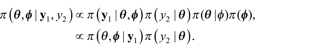
Intuitively, we can think of
where
Importantly,
We note that though we target the same constrained posterior distribution as Zhang and Bryant (2020), our approach is distinct in the implementation in that we do not obtain samples from this posterior distribution in a single step, such as with an MCMC algorithm as implemented in Zhang and Bryant (2020). Rather, our approach allows for first obtaining samples from an unbenchmarked model (not necessarily using MCMC, hence greater flexibility and potential speed gains) and benchmarking in a second step involving either a rejection sampler or a Metropolis-Hastings algorithm.
3.4.1. Rejection Sampler
In a rejection sampling framework, we can obtain samples from
Generate
Accept
Otherwise, return to Step 1.
This rejection sampling approach targets the same constrained posterior distribution as the fully Bayesian benchmarking approach of Zhang and Bryant (2020) but in a computationally straightforward manner. As the rejection sampling approach only requires posterior draws from an unbenchmarked posterior distribution, this allows practitioners to use a wider array of computation tools to conduct fully Bayesian benchmarking, even when benchmarking constraints are nonlinear. A relevant example of such a computational tool is INLA, which does not allow for non-linear predictors, and therefore INLA cannot directly incorporate the likelihood for a nonlinear benchmark into the model (Rue et al. 2009). Crucially, unbenchmarked posterior samples can be generated from an INLA analysis.
3.4.2. Metropolis-Hastings
The rejection sampling approach to fully Bayesian benchmarking may be inefficient in cases where benchmarks are far from the population aggregated estimates from an unbenchmarked model. One potential way to address this inefficiency is to instead use an independence Metropolis-Hastings (MH) algorithm (Tierney 1994). Intuitively, we can fit an adjusted unbenchmarked distribution that has been shifted toward the national benchmarks and correct for this shift in the acceptance rate. This serves to increase the proportion of accepted samples relative to using the unbenchmarked distribution as a proposal distribution by moving the proposal distribution closer to where the constrained posterior should be.
Here we present one example of an adjusted unbenchmarked distribution that can be used as a proposal distribution, and show how the shift can be corrected for in the acceptance rate. Note that we assume in this example that the unadjusted, unbenchmarked model we would want to fit has a fixed intercept β with a flat prior,
Suppose that area-level parameters are linked to a mean model
where
In this framework, we can obtain samples from the same benchmarked posterior distribution
Initalize
Sample
Compute the acceptance probability
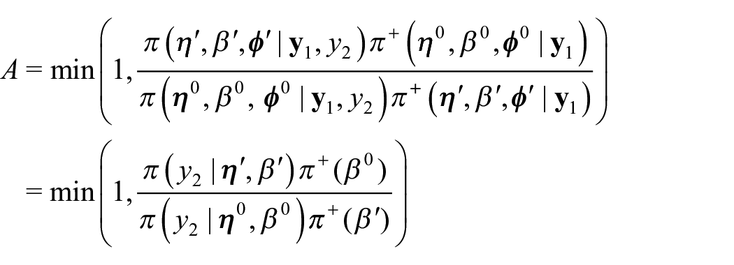
With probability A, accept the proposed value
Just as with the rejection sampling approach, the MH approach targets the same constrained posterior distribution as the fully Bayesian benchmarking approach of Zhang and Bryant (2020) but in a computationally convenient manner.
3.4.3. Convergence Diagnostics
While the MH algorithm may have a higher acceptance rate than the rejection sampling approach (and therefore greater computational speed), additional care must be taken to ensure that the algorithm has mixed and converged properly. Though not a convergence diagnostic, one basic check is to aim for an acceptance rate near 23.4%, as suggested in Gelman et al. (1997) as the optimal acceptance rate under normal posteriors for random walk Metropolis algorithms. It may be desirable to vary the prior
A common convergence diagnostic for MCMC sampling is the potential scale reduction factor
Following the guidelines in Vehtari et al. (2021),we recommend running at least four chains if using the MH approach to benchmarking that we propose. Aiming for a rank-normalized split-
3.4.4. Limitations
Despite the potential improvements in speed from the MH approach over the rejection sampler approach, both methods may still be inefficient in cases where benchmarks are far from the population aggregated estimates from an unbenchmarked model. It may be necessary in such cases to use an approach such as Zhang and Bryant (2020)’s in order to produce benchmarked estimates. However, we caution that if the proportion of accepted samples is very small this may be indicative of inconsistencies between the two data sources, and model elaboration may be required in this case.
Additionally, the rejection sampling and MH approaches cannot benchmark estimates with zero variance, as the likelihood
A final consideration with the MH approach is that using this algorithm with the suggested proposal distribution will not allow for comparison between the resulting benchmarked estimates and the unbenchmarked estimates from the unadjusted, unbenchmarked model, without separately fitting an unadjusted, unbenchmarked model. In some official statistics settings it may be desirable or even required to compare benchmarked estimates to unbenchmarked estimates, and if the time it takes to separately fit an unadjusted, unbenchmarked model is time-consuming, the MH approach may be impractical.
4. Simulation
To demonstrate the improved computational speed of our approach compared to Zhang and Bryant (2020), we compare run-times for our approach used with INLA to that of Zhang and Bryant (2020) implemented in Stan; a probabilistic programming language that uses a variant of Hamiltonian Monte Carlo to do full Bayesian inference (Carpenter et al. 2017). We chose not to compare the computational speed of our approach to that of Datta et al. (2011) or the raking approach, as both of those benchmarking approaches target different benchmarked estimates than our proposed method. Note, however, that both the raking and benchmarked Bayes estimate approach will be the fastest approach to benchmarking in general, as they involve a very quick step to adjusting unbenchmarked draws/estimates, and do not rely on acceptance rates (as our methods do to achieve a reasonable number of effective samples) or MCMC methods.
We simulate unit-level (cluster) binomial observations, using the nine provinces (small areas) of South Africa as our spatial structure. For each simulation setting, binomial probabilities were given by
The unbenchmarked model we fit to the generated data is the unit-level model used in our application to South Africa (and described in Section 2.1.2), where we have binomial observations for clusters c within area i. Let
where
The modified unbenchmarked model, used for the MH algorithm is the same as above with the exception of the prior for the intercept being
and the proposed rejection sampler and MH algorithm approaches are carried out as described in Sections 3.4.1 and 3.4.2. Code for reproducing the simulation can be found at https://github.com/taylorokonek/benchmarking-paper-sim.
To fairly compare run-times, we compare the time it takes to:
Fit the fully Benchmarked model per Zhang and Bryant (2020) in Stan, and obtain a bulk-ESS of 1,000.
Fit the unbenchmarked model in INLA, draw posterior samples, and obtain 1,000 accepted samples using the rejection sampler.
Fit the modified unbenchmarked model in INLA, draw posterior samples, and obtain a bulk-ESS of 1,000 using the MH algorithm.
For both Stan and the MH algorithm, we run four chains with 1,000 burn-in samples each, and the appropriate number of samples after to obtain the desired bulk-ESS.
In Figure 1 we compare methods under the setting
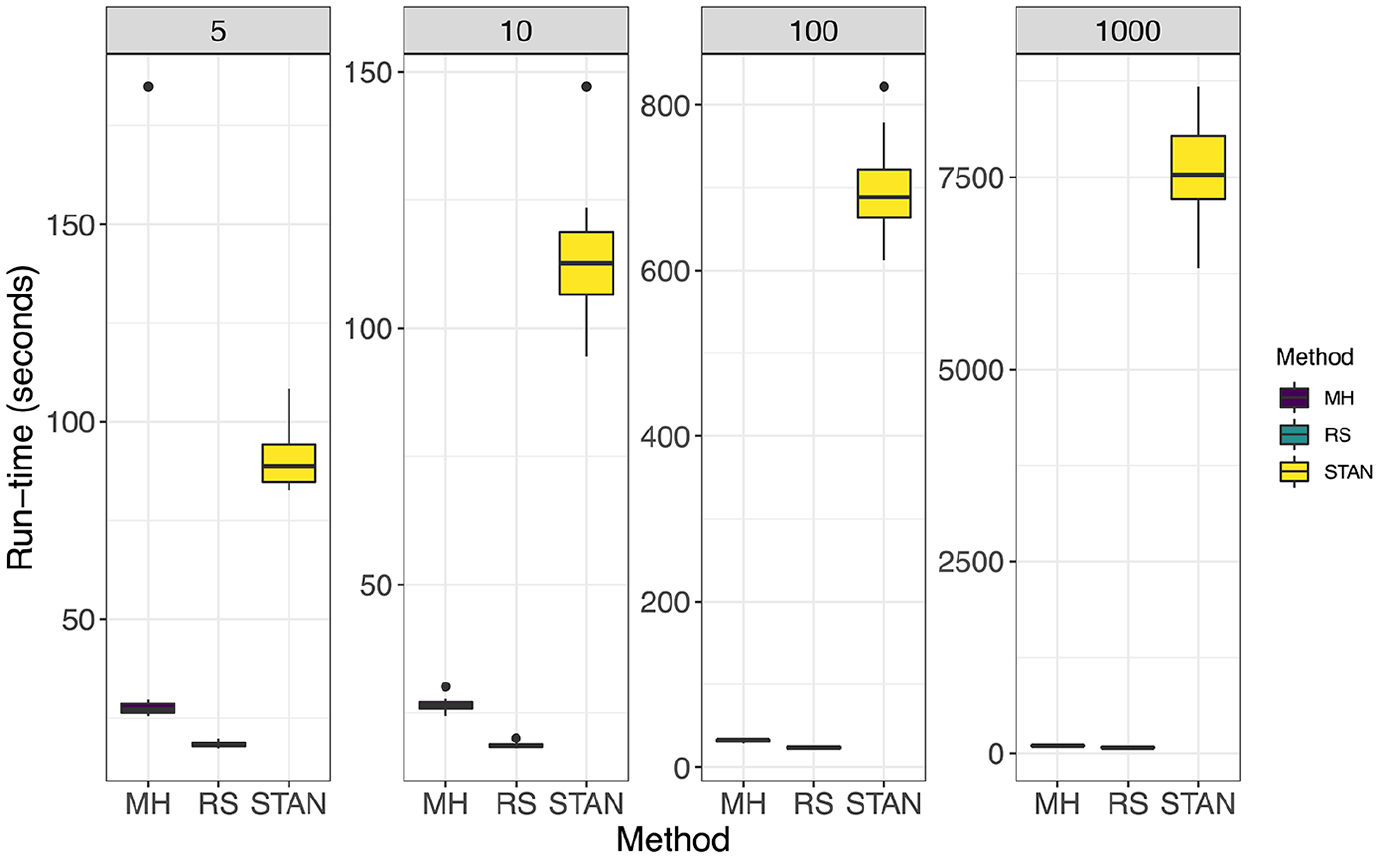
Setting:
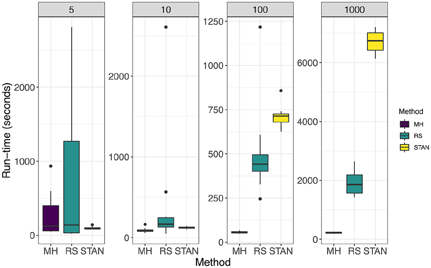
Setting:
5. Application
Below we describe the data, models, and software used in the HIV prevalence application. The application to U5MR is in Section 2 of the Supplemental data.
We fit both area-level and unit-level models to demonstrate the flexibility of our proposed method over existing computational software. As noted in Section 3.3, there is currently no available implementation of the fully Bayesian benchmarking approach described in Zhang and Bryant (2020) to unit-level models. As unit-level models are commonly used in LMICs when estimating public health outcomes in an official statistics setting (Wakefield et al. 2020; Wu et al. 2021), it is important for practitioners to have a method available to conduct fully Bayesian benchmarking with unit-level models without needing to write their own MCMC algorithm. We demonstrate that our proposed method is readily applicable to both area- and unit-level models.
For our unbenchmarked area-level model, we consider the spatial Fay-Herriot model defined in Mercer et al. (2015). The model is detailed in Section 2.1.1. The Fay-Herriot model is one of the most well-known small area models, that directly incorporates aspects of the survey design using a transformed survey-weighted estimate and an iid random effect to increase precision of the resulting estimates (Fay and Herriot 1979). The spatial extension incorporates both an iid random effect and an additional structured spatial random effect to further capture spatial dependency in the observations (Mercer et al. 2015).
For our unbenchmarked unit-level model, we consider a hierarchical Bayesian model with a spatial random effect term for the application to HIV prevalence, and the model currently used to produce subnational estimates of U5MR for the UN IGME (Wu et al. 2021). The model is detailed in Subsection 2.1.2. Of note, these unit-level models do not directly account for the survey design like the area-level model. It has been suggested that, when possible, the inclusion of covariates related to the survey design could be included in such a model-based framework to account for the survey design (Wakefield 2013; Wu et al. 2021). One example of this can be found in Paige et al. (2022), though as noted in Wakefield et al. (2020), in many surveys conducted in LMICs the covariates corresponding to the survey design may be unavailable.
5.1. Data
Spatial boundary files for South Africa are obtained from GADM, the Database of Global Administrative Areas (Database of Global Administrative Areas [GADM] 2019).
We estimate HIV prevalence in South Africa from the 2016 South Africa DHS survey. The survey followed a multi-stage, stratified design, and was designed to provide estimates at the Administrative 1 (admin1) level, which consists of nine provinces, which we considered to be our small areas for this application. Subareas within each of the nine provinces were assigned urban/farm/traditional area status, and therefore resulted in twenty-six strata, as the Western Cape province does not have a traditional area geotype. The sampling frame was established from the 2011 census, and 750 enumeration areas (primary sampling units, PSUs) were selected across strata. The second stage of sampling sampled dwelling units, or households, from the enumeration areas, and every individual within the household (if available) was included in the survey. Only men and women aged fifteen to forty-nine were included in the HIV dataset. Households within a given enumeration area are given a single geographic location, and we denote these as clusters from here on. GPS coordinates are displaced by up to 2 km for urban clusters and 5 km for rural clusters, but are never displaced outside of their area of stratification.
Of note, all nine small areas (provinces) for this application contained at least one binomial observation. The number of PSUs in each small area ranged from 56 to 88. The binomial counts within each primary sampling unit ranged from 0 to 11, with totals in each primary sampling unit ranging from 1 to 30. The distribution of observed binomial proportions in each PSU can be seen in Figure 3.
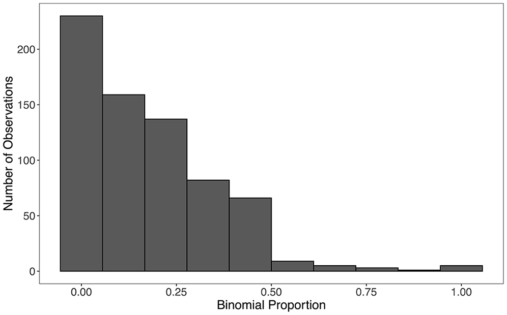
Observed binomial proportions in each PSU.
We obtain a national level estimate for 2016 in South Africa from the national Thembisa model, an HIV epidemic projection model that produces the official estimates published by UNAIDS for South Africa (Johnson, May, et al. 2017; Mahy et al. 2019; Stover et al. 2019). The national level estimate of HIV prevalence for 2016 in South Africa is 17.1%, with a 95% confidence interval of (15.6%, 18.3%). For the benchmark likelihood for the fully Bayesian benchmarking approaches we need a standard error for this benchmarked estimate, which we take to be (18.3−17.1) / 1.96 = 0.61 based on the assumption that the national level estimate is asymptotically normally distributed. The Thembisa model incorporates data from five Human Sciences Research Council (HSRC) surveys conducted from 2002 to 2017, the 2016 DHS survey, Antenatal Sentinel HIV and Syphilis Surveys, and antiretroviral therapy coverage data. Although the DHS survey is included in the model for the benchmarks, we treat this as an external benchmarking scenario as multiple other data sources are included in the national model as well.
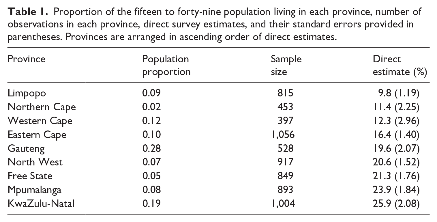
The population count data we use for our HIV application comes from the provincial Thembisa model (Johnson, Dorrington, and Moolla 2017). We use this specific population data as they are currently used in UNAIDS models of subnational HIV prevalence in South Africa (Eaton et al. 2021). In Figure 4, we plot the spatial distribution of individuals aged fifteen to forty-nine (the population in our HIV example) in 2016 in South Africa; that is, out of all people aged fifteen to forty-nine in South Africa, the proportion of that sub-population who live in each region is displayed. The population proportions are also present in Table 1, along with the number of observations in each province and their direct, survey-weighted estimates.
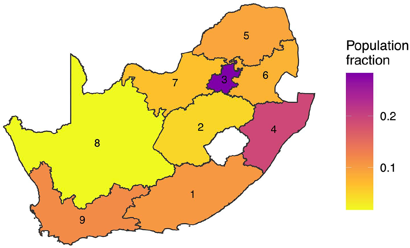
Proportion of the fifteen to forty-nine population living in each province. These proportions are the weights used to aggregate province level estimates to the national level. Provinces are labeled in alphabetical order: (1) Eastern Cape; (2) Free State; (3) Gauteng; (4) KwaZulu-Natal; (5) Limpopo; (6) Mpumulanga; (7) NorthWest; (8) Northern Cape; (9) Western Cape.
Proportion of the fifteen to forty-nine population living in each province, number of observations in each province, direct survey estimates, and their standard errors provided in parentheses. Provinces are arranged in ascending order of direct estimates.
5.2. Benchmarked Models
We compute benchmarked estimates using the fully Bayesian approach of Zhang and Bryant (2020), the proposed approaches, and the raking approach. This allows us to show: (1) the benchmarked estimates from our proposed approaches are identical to those from the Zhang and Bryant (2020) method, and (2) a comparison of the benchmarked estimates from the proposed approach to what is currently used in practice (raking) by the UN when estimating both HIV Prevalence and U5MR subnationally (Eaton et al. 2021; Wu et al. 2021).We do not compute benchmarked estimates using the benchmarked Bayes estimate approach, as we have noted in Section 3.1 that it is inappropriate for these applications. We obtain credible intervals for our benchmarked and unbenchmarked estimates using draws from the posterior distributions.
5.2.1. Approaches
5.2.1.1. Raking
We obtain posterior medians
5.2.1.2. Fully Bayesian
Using weights
with
5.2.1.3. Fully Bayesian: Rejection sampler
We obtain
5.2.1.4. Fully Bayesian: Metropolis-Hastings algorithm
We obtain
5.3. Model Validation
As we view benchmarking as a necessary adjustment needed to an existing unbenchmarked model in an official statistics setting, we choose to validate the unbenchmarked models we fit prior to benchmarking. Note that if benchmarking is instead viewed as a way to reduce potential bias in subnational estimates, model validation may need to be done to the resulting benchmarked models as opposed to the unbenchmarked models.
Wakefield et al. (2020), among others (Osgood-Zimmerman et al. 2018; Wu et al. 2021), suggest that one way to approach model validation in small area models in a survey setting is to check whether the direct estimates in each area lie within an uncertainty interval surrounding the posterior means of the predictive distribution in that area. In a survey setting in LMICs, the direct estimates are considered the gold standard; hence, model-based estimates should not stray too far from the direct estimates. This also gives one an idea of average coverage across areas: 80% of the direct estimates (left out data) should lie within 80% credible intervals based on the predictive distribution.
We take this approach to model validation for both our unbenchmarked area-level and unit-level models. Details and figures containing the results of model validation for the HIV application can be found in Subsection 1.4 of the Supplemental data, and Subsection 2.6 of the Supplemental data for the U5MR application.
5.4. Computation
As the novelty of our approach is computational, we chose the statistical programs used in the application to demonstrate the flexibility of our approach compared to the fully Bayesian approach of Zhang and Bryant (2020).
For the approach described in Zhang and Bryant (2020), we implement models in Template Model Builder (TMB) (Kristensen et al. 2016). TMB is a flexible modeling tool that takes advantage of Laplace approximations for computational efficiency, and allows users to specify a wide variety of models in C++. For a review of TMB, see Section 4 of Osgood-Zimmerman and Wakefield (2021). Importantly, TMB allows users to specify nonlinear predictors, unlike INLA, which is needed for implementing the fully Bayesian benchmarking approach of Zhang and Bryant (2020) in settings with binary outcomes. Of note, TMB still requires model-specific implementations, and therefore does not have as nice of an interface as other programs (such as INLA, which we will describe below).
To show that the results from our proposed method are identical to those from the Zhang and Bryant (2020) method, we also fit the unbenchmarked HIV models in our application using TMB. This ensures that the posterior distributions are directly comparable. Note that our proposed method could have been implemented using INLA to fit the unbenchmarked model as well, but as INLA uses a different Laplace approximation than TMB, the results would not have been exactly, directly comparable.
For our U5MR application, we fit all unbenchmarked models in INLA to show that our proposed method is compatible with the software currently used to produce official estimates of U5MR for the UN IGME. INLA is an appealing, alternative Laplace approximation program for obtaining posterior distributions for latent Gaussian models (Rue et al. 2009). Unlike TMB, INLA does not allow users to specify nonlinear predictors. Since our proposed approach does not require the use of such nonlinear predictors for the benchmarking constraint by taking advantage of a two-step procedure, we implement the models for our U5MR application using INLA to demonstrate the benefit of the increased flexibility of our approach to accommodate fast Laplace approximation techniques such as INLA.
5.5. Results
In Figure 5 and Table 2, we display national level estimates from Thembisa, the unbenchmarked, and benchmarked results from the unit-level model. Results from the area-level model are very similar to those from the unit-level model, and can be found in Table 2 as well, with more detailed results in Subsection 1.2 of the Supplemental data and direct comparisons between the unit-level and area-level models found in Subsection 1.3 of the Supplemental data. We see that the fully Bayesian benchmarking approaches produce essentially identical results, and that they are a compromise between the likelihood given by the national level benchmark and the unbenchmarked posterior estimate. The raking approach enforces exact benchmarking, which is evidenced by the overlap between the density of the Thembisa national estimate and that of the benchmarked method’s national aggregated estimate. The fully Bayesian rejection sampler accepts 7.6% of unbenchmarked samples using the unit-level model, and 8.6% of unbenchmarked samples using the area-level model. The fully Bayesian MH approach accepts 18.8% of unbenchmarked samples using the unit-level model, and 18.9% of unbenchmarked samples using the area-level model.
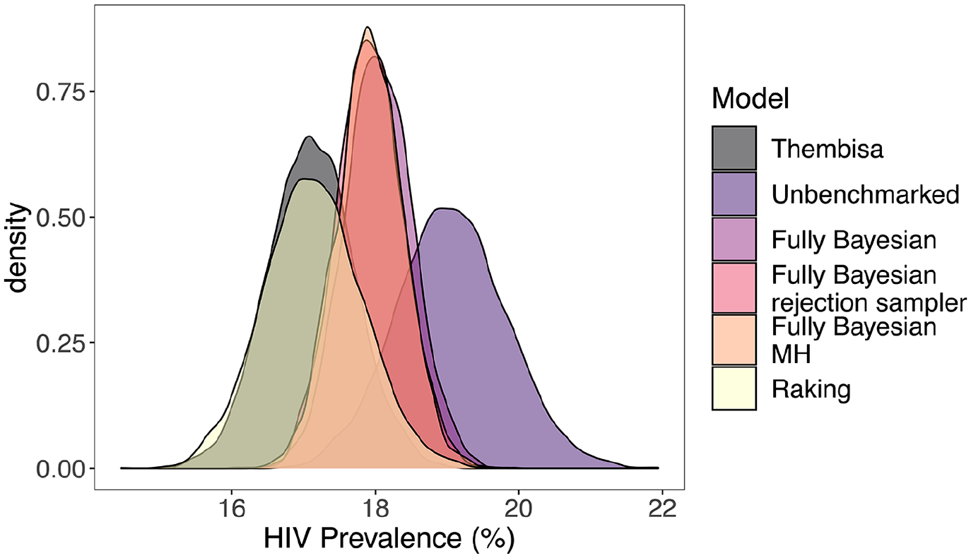
Aggregated national level HIV prevalence estimates from Thembisa, unbenchmarked, and benchmarked results from the unit-level model. The fully Bayesian model refers to the approach described in Zhang and Bryant (2020), and the fully Bayesian rejection sampler and fully Bayesian MH refer to the proposed approaches. All densities are based on five thousand samples.
Aggregated national level hiv prevalence estimates from Thembisa, unbenchmarked, and benchmarked results from the unit-level and area-level models. 95% Credible intervals are given next to posterior medians.
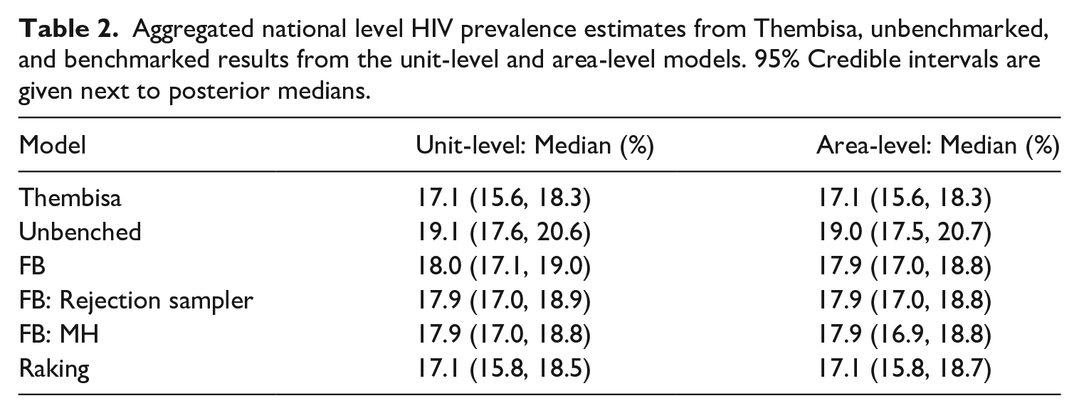
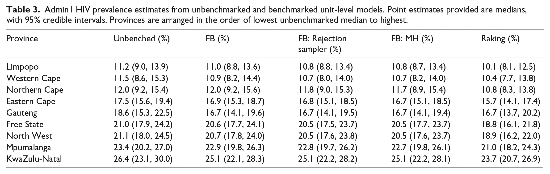
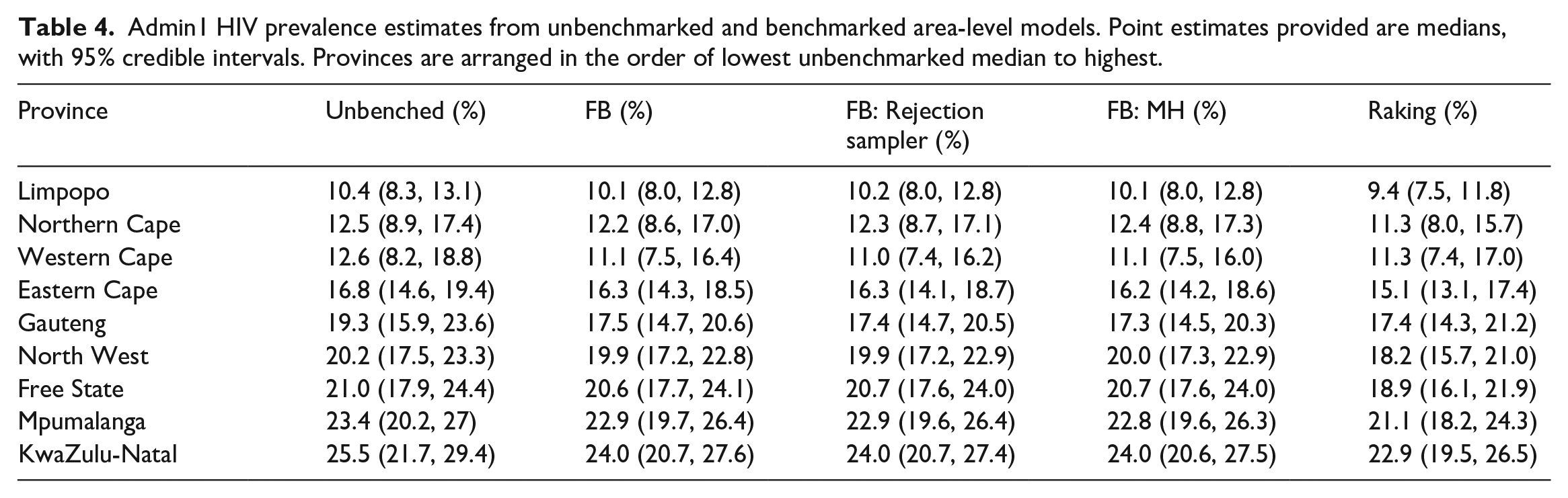
Figure 6 and Table 3 display the subnational breakdown of benchmarked and unbenchmarked estimates from the unit-level model. Of note, the benchmarked posterior medians and credible intervals for the fully Bayesian approaches look roughly identical (as they should), and the posterior distributions for each province from the raking approach are all slightly lower than those from the fully Bayesian approaches. This difference is due to the raking approach enforcing the benchmarking constraint exactly, thus pulling the unbenchmarked estimates down farther than the fully Bayesian approaches, as the national benchmark is lower than the unbenchmarked national estimate. Though more difficult to see, the fully Bayesian approach treats regions with more uncertainty differently than those with less uncertainty. In particular, note that in the Eastern Cape province the fully Bayesian benchmarked posterior medians are not as different from the unbenchmarked median as in the Gauteng province, where uncertainty is much higher in the unbenchmarked estimate. This is opposed to the raking approach, which shifts all estimates by the same multiplicative constant, regardless of uncertainty. Table 4 displays the subnational breakdown of benchmarked and unbenchmarked estimates from the area-level model, with additional results in Subsection 1.2 of the Supplemental data.
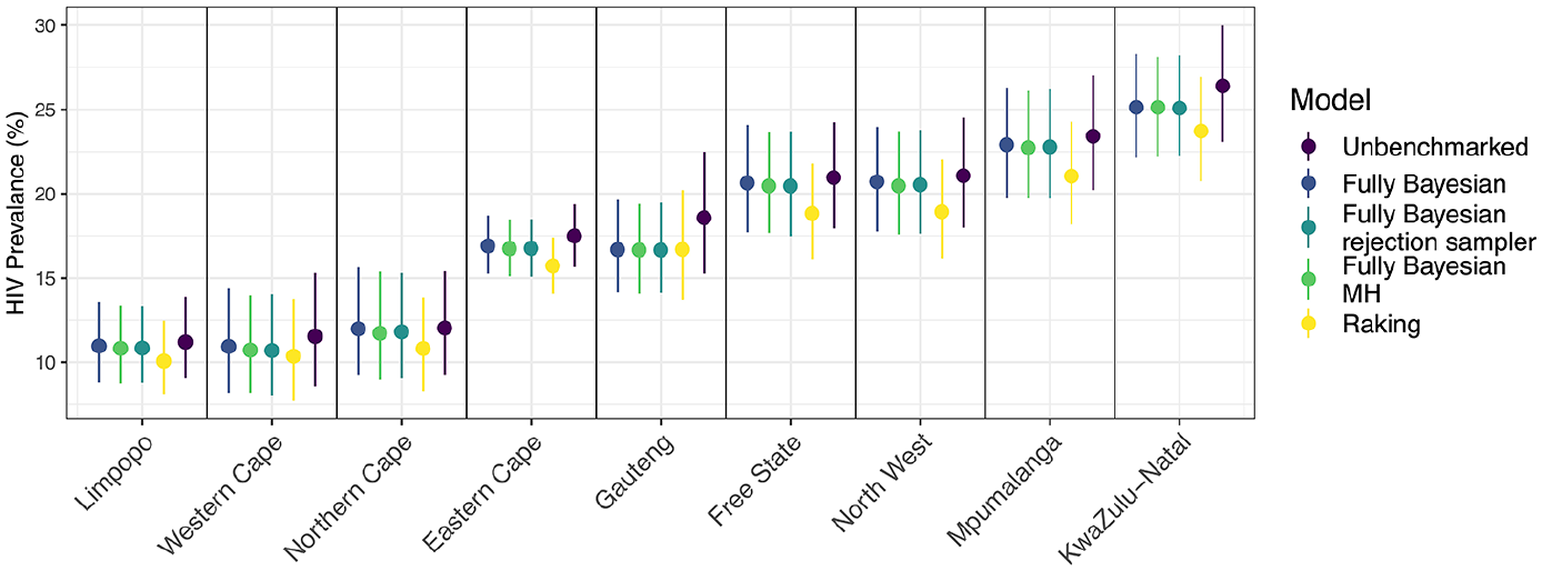
Comparison of HIV Prevalence estimates from benchmarked and unbenchmarked unit-level models at a subnational level. Error bars correspond to 95% credible intervals, and provinces are arranged from left to right in order of unbenchmarked median.
Admin1 HIV prevalence estimates from unbenchmarked and benchmarked unit-level models. Point estimates provided are medians, with 95% credible intervals. Provinces are arranged in the order of lowest unbenchmarked median to highest.
Admin1 HIV prevalence estimates from unbenchmarked and benchmarked area-level models. Point estimates provided are medians, with 95% credible intervals. Provinces are arranged in the order of lowest unbenchmarked median to highest.
The model validation results for the HIV application for both unit- and area-level models suggest that both models are reasonably well-suited to the data. We compare posterior medians of the predictive distribution in each area (having left that area out of model fitting) to the direct estimate in each area, respectively. The 80% credible intervals capture
Additional plots and tables, including those for the area-level model, can be found in Section 1 of the Supplemental data.
5.6. U5MR
The results for the U5MR application are in Section 2 of the Supplemental data.
6. Discussion
In this paper we have summarized existing benchmarking approaches and their benefits and drawbacks with regard to data with rare binary outcomes in LMICs. We consider benchmarking methods that make use of a benchmarking constraint via one-step or two-step approaches, and pay particular attention to the resulting interpretation of the benchmarked estimates, the ease of uncertainty quantification, the acknowledgment of uncertainty in national estimates, the use of non-linear constraints, and computational tractability. We believe that the proposed rejection sampling and MH approaches to fully Bayesian benchmarking provide a desirable balance all of these concerns, and provide alternative computational approaches to the one-step, fully Bayesian benchmarking method developed by Zhang and Bryant (2020), which in many cases may be inflexible with regards to modeling choice and computational tractability, while targeting the same benchmarked, posterior distribution.
We show via an application of various benchmarking approaches to an HIV prevalence example that the proposed two-step approaches to fully Bayesian benchmarking produce the same benchmarked estimates as the one-step Zhang and Bryant (2020) approach, and that the resulting estimates are a compromise between the national level estimate and unbenchmarked estimates. The rejection sampling and MH approaches allow us to take advantage of potentially faster computational programs than traditional MCMC samplers, such as INLA or TMB, as evidenced by our application to U5MR. Inference for spatial models (continuous models especially) using MCMC methods is computationally challenging, and our approach allows users to conduct fully Bayesian benchmarking while relying on Laplace approximation methods for inference that are more suited for such models (Osgood-Zimmerman and Wakefield 2021). Additionally, the rejection sampling and MH approaches are easily applied to both unit-level and area-level models, as evidenced by both our HIV and U5MR applications. Though not explored in this paper, additional algorithms could be considered to similarly obtain benchmarked posterior distributions in a two-step fashion, such as the sampling-importance resampling approach (see Subsection 10.4 of Gelman et al. (2013)).
Though the purpose of this paper was not to provide an in-depth review of small area models in LMICs, one reviewer noted that our unit-level models do not directly account for the survey design. This point should not go unnoticed, and as with any application involving survey data, careful consideration should be given the survey design even if a model-based approach is required for adequate precision.
There are several limitations with the proposed approaches to fully Bayesian benchmarking. The first and potentially most pressing is the inability to conduct exact benchmarking, which may be required in some settings and is especially relevant if national benchmarks come from a census, though censuses have uncertainty in practice. Scenarios where true exact benchmarking is required are rare in an LMIC context. While we note that exact benchmarking can be approximated via the proposed approaches, it will likely be computationally inefficient. The one-step approach to fully Bayesian benchmarking may be a more useful approach if exact benchmarking is required, or a posterior projection approach using a loss function that respects the bounds on the estimates that are being benchmarked.
Additionally, our method does not account for uncertainty in the population count data. The population data used in our applications did not have reported uncertainty. If uncertainty for population count data were available, this would ideally be incorporated into the likelihood for the benchmarking constraint. Worldpop has recently started quantifying uncertainty in population data for select countries in their bottom-up Bayesian models, which may be of interest to include in future applications (Leasure et al. 2020).
Footnotes
Funding
The author(s) disclosed receipt of the following financial support for the research, authorship, and/or publication of this article: Research reported in this publication was supported by the National Institute Of Allergy And Infectious Diseases of the National Institutes of Health under Award Number R37AI029168. The content is solely the responsibility of the authors and does not necessarily represent the official views of the National Institutes of Health.
Supplemental Material
Supplemental material for this article is available online.
Received: March 21, 2022
Accepted: December 7, 2023
References
Supplementary Material
Please find the following supplemental material available below.
For Open Access articles published under a Creative Commons License, all supplemental material carries the same license as the article it is associated with.
For non-Open Access articles published, all supplemental material carries a non-exclusive license, and permission requests for re-use of supplemental material or any part of supplemental material shall be sent directly to the copyright owner as specified in the copyright notice associated with the article.