
Abstract
County level estimates of mean sheet and rill erosion from the Conservation Effects Assessment Project (CEAP) are useful for program development and evaluation. Since county sample sizes in the CEAP survey are insufficient to support reliable direct estimators, small area estimation procedures are needed. The quantity of water runoff is a useful covariate but is unavailable for the full population. We use an estimate of mean runoff from the CEAP survey as a covariate in a small area model with sheet and rill erosion as the response. As the runoff and sheet and rill erosion are estimators from the same survey, the measurement error in the covariate is important as is the correlation between the measurement error and the sampling error. We conduct a detailed investigation of small area estimation in the presence of a correlation between the measurement error in the covariate and the sampling error in the response. In simulations, the proposed predictor is superior to small area predictors that assume the response and covariate are uncorrelated or that ignore the measurement error entirely.
1. Introduction
The Conservation Effects Assessment Project (CEAP) is a program comprised of several surveys that are intended to evaluate the environmental impacts of agricultural production. We consider data from a CEAP survey of cropland that was conducted over the period 2003 to 2006. An important variable collected in CEAP is sheet and rill erosion (soil loss due to the flow of water). County estimates of sheet and rill erosion can improve the efficiency of allocation of resources for conservation efforts. Sample sizes in CEAP are too small to support reliable direct county estimates. Past analyses have explored a variety of issues that arise in the context of small area estimation using CEAP data (Berg and Chandra 2014; Berg and Lee 2019; Erciulescu and Fuller 2016; Lyu et al. 2020).
Traditional small area estimation procedures utilize population-level auxiliary information from censuses or administrative databases (Jiang and Lahiri 2006; Pfeffermann 2013; Rao and Molina 2015). A critical assumption underlying the seminal Fay and Herriot (1979) predictor is that one can condition on the observed value of the covariate. As discussed in Lyu et al. (2020), the task of obtaining covariates that are related to sheet and rill erosion and are known for the full population of cropland of interest is difficult. Use of variables collected in the CEAP survey as covariates is therefore desirable. We use an estimate of mean water runoff from the CEAP survey as a covariate in an area level model with sheet and rill erosion as the response. As the covariate and response are both estimates from the CEAP survey, the analysis should recognize not only the sampling error in the covariate but also the correlation between the covariate and the response.
If the covariate is an estimator from a sample survey, naive application of standard Fay-Herriot procedures can lead to erroneous inferences (Arima et al. 2017; Bell et al. 2019). A widely used technique to model sampling error in the covariate is to employ either a structural (Arima et al. 2012; Ghosh et al. 2006; Torabi 2012; Torabi et al. 2009) or a functional (Datta et al. 2010; Ghosh and Sinha 2007; Torabi 2011) measurement error model. In the structural model, the latent covariate is stochastic, while the functional model treats the unobserved covariate as fixed (Carroll et al. 2006; Fuller 2009).
Ybarra and Lohr (2008) develops predictors for an area level model in which a covariate is subject to functional measurement error. Arima et al. (2015), Arima et al. (2017), and Burgard et al. (2021) extend Ybarra and Lohr (2008) to bivariate and Bayesian frameworks. Burgard et al. (2020) conducts an analysis of the model of Ybarra and Lohr (2008) under the stronger assumption that the random terms have normal distributions. Bell et al. (2019) compares the properties of functional and structural measurement error models to the naive Fay-Herriot model. Mosaferi et al. (2023) extends Ybarra and Lohr (2008) to lognormal data. All of these works assume that the measurement error in the covariate and the sampling error in the response are uncorrelated.
Models in which the measurement error and the sampling error are correlated have received little attention in the small area estimation literature. Franco and Bell (2022) defines a bivariate model that is equivalent to a structural model with a correlation between the measurement error and the sampling error. We adopt the functional modeling approach, which, unlike the structural model, requires no assumptions about the distribution of the latent covariate. Kim et al. (2015) permits a correlation between the covariate and response but conceptualizes the parameter of interest as the unobserved value of a covariate that is measured with error. Ybarra (2003) generalizes the functional measurement error model of Ybarra and Lohr (2008) to allow for a correlation between the measurement error and the sampling error. Burgard et al. (2022) uses likelihood-based arguments to derive a predictor for a model in which the measurement error and the sampling error are correlated.
We conduct a thorough analysis of a model in which the measurement error and the sampling error are correlated. Our work expands on Ybarra (2003) in several dimensions. We conduct extensive simulation studies in a framework where the measurement error in the covariate is correlated with the sampling error in the response. We rigorously discuss the theoretical properties of the predictors with estimated parameters. Further, we provide comprehensive software at https://github.com/emilyjb/SAE-Correlated-Errors/.
The rest of this manuscript is organized as follows. We derive a predictor using properties of the bivariate normal distribution in Section 2.1. We propose estimators of the fixed model parameters in Section 2.2, and we study the theoretical properties of the proposed estimators. Then, we derive the mean squared prediction error (MSPE) of the proposed predictor. We also conduct extensive simulations to assess the properties of the proposed procedures in Section 3. We apply the proposed method to data from the CEAP survey in Section 4. We conclude in Section 5.
2. Model and Predictor
We define an area-level model, where the measurement error in the covariate is correlated with the sampling error in the response. We denote the true, unknown value of the covariate by
The parameter of interest is

where
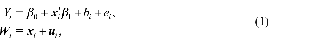
and
Typically,
The component
Remark 1: The model in (1) has strong connections to other models in the small area estimation literature. The model is identical to the model of Ybarra (2003). If
Remark 2: In many situations, as in the CEAP data analysis of Section 4, the observed covariate is an estimator from a sample survey. In this case, the error in the observed covariate is a sampling error. Because the model (1) has the form of a measurement error model, we refer to the random term
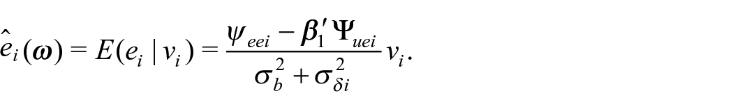
2.1. Predictor as a Function of the True Model Parameters
We first define a predictor as a function of the unknown

Then, using properties of the bivariate normal distribution (as explained in Appendix A),
where

where
The MSPE of
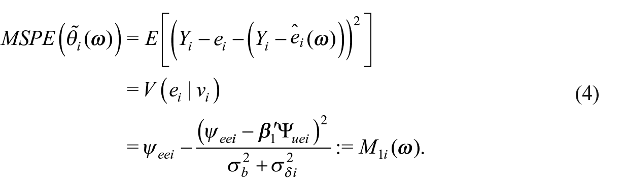
In (4),
Remark 3: We use the properties of the bivariate normal distribution to derive the predictor (3). A different way to develop a predictor is to find the convex combination of
Remark 4: Burgard et al. (2022) define a predictor for a generalization of the model (1). The predictor proposed in (3) differs from that of Burgard et al. (2022). In the supplement, we provide empirical evidence that the predictor (3) is more efficient than the predictor of Burgard et al. (2022).
2.2. Estimation of Parameters
We require estimators of
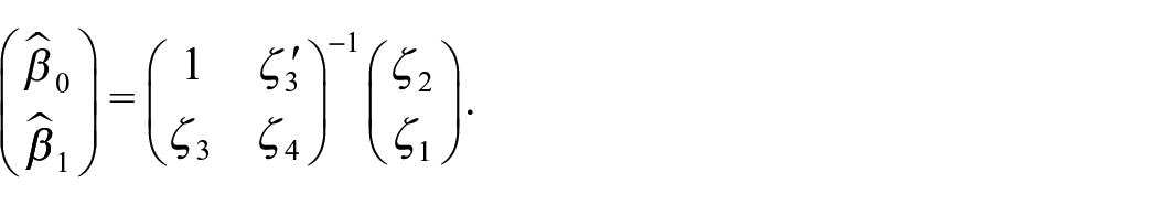
Theorem 1 of Appendix B states that the estimator of the regression coefficients is consistent, where we simplify and only consider a univariate covariate. We outline the proof of Theorem 1 in Appendix B and provide further details in the Supplemental Material.
The estimator of
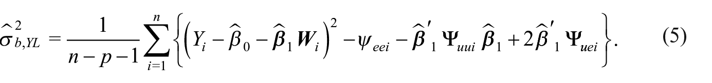
A drawback of the estimator (5) is that it can be negative. Thus, we use a profile likelihood.
We define the profile likelihood for estimating
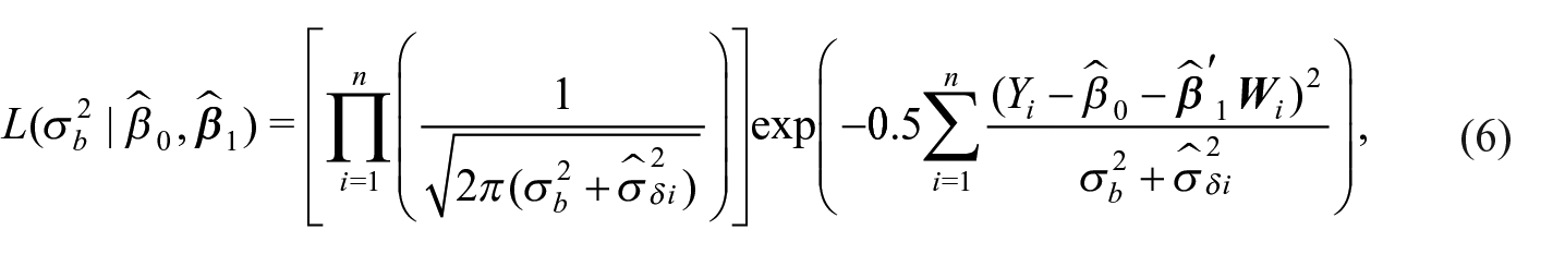
where
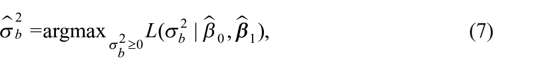
where the maximization is over the parameter space for
Remark 5: For the estimation of
Remark 6: It may be observed that we use a likelihood-based estimator of
2.3. Predictors with Estimated Parameters
We evaluate the predictor (3) at the estimator of

where
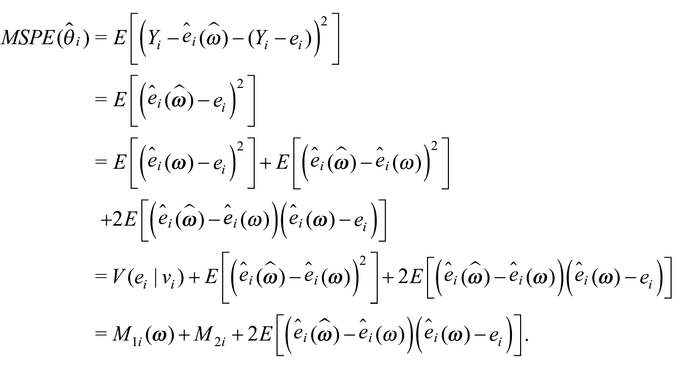
The first term,
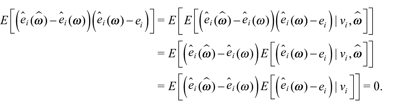
The final equality holds because

We use a plug-in estimator of
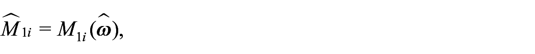
where
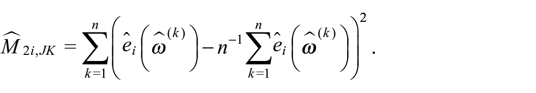
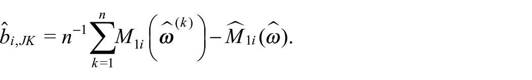
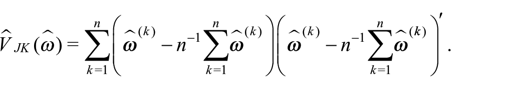
The jackknife estimate of the bias of the estimator of
The estimator of the MSPE is then defined as

Remark 7: The simplifying assumption that
Remark 8: Alternatives to the jackknife variance estimator are Taylor linearization and the bootstrap. For this model, Taylor linearization is possible, but the operations are tedious. We prefer the jackknife relative to Taylor linearization for simplicity of implementation.
Remark 9: We use the assumption of normality when formulating the predictor and when proving that the parameter estimators are consistent. The procedures, however, do not rely heavily on the normality assumption. The development of the predictor in Ybarra (2003) as the optimal convex combination between the direct estimator and
3. Simulations
We conduct simulations with two goals. The first is to understand the effect of the nature of
As one of the simulation objectives is to understand the effects of the form of
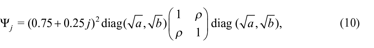
for
We define eight simulation configurations by four combinations of
We refer to the procedure proposed in Section 2 as ME-Cor. We compare the proposed procedure to two primary competitors. One competitor is the approach of Ybarra and Lohr (2008), which assumes that
We do not include the predictor outlined in Ybarra (2003) in the simulations for two main reasons. One is that the predictor of Ybarra (2003) is not fully developed for the case of a correlation between the measurement error and the sampling error. The other is that we do not view the procedure of Ybarra (2003) as a competitor to our approach. Instead, our objective is to build on the predictor of Ybarra (2003) and study its properties in more detail.
We also do not compare our predictor to a predictor for a bivariate model in which the covariate is included as a second response variable. As discussed in Section 1, Franco and Bell (2022) considers a bivariate modeling approach. Their approach is equivalent to a structural measurement error model with no covariates. We prefer to remain in the framework of functional measurement error. Therefore, we do not include a comparison to a predictor based on a bivariate model.
3.1. Normal Distributions, Unequal
We first simulate data with normally distributed random components, as specified in model (1). We use the unequal
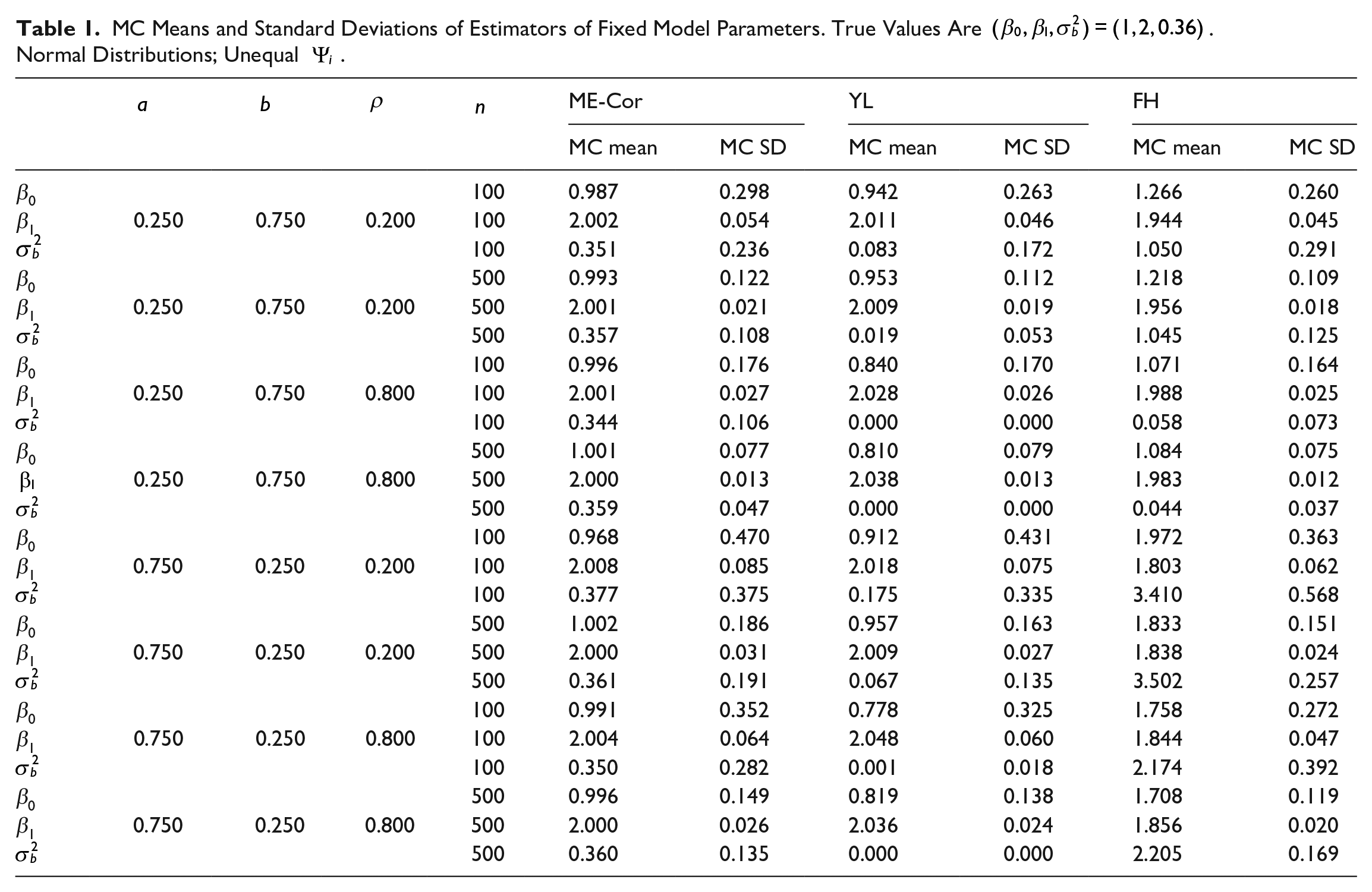
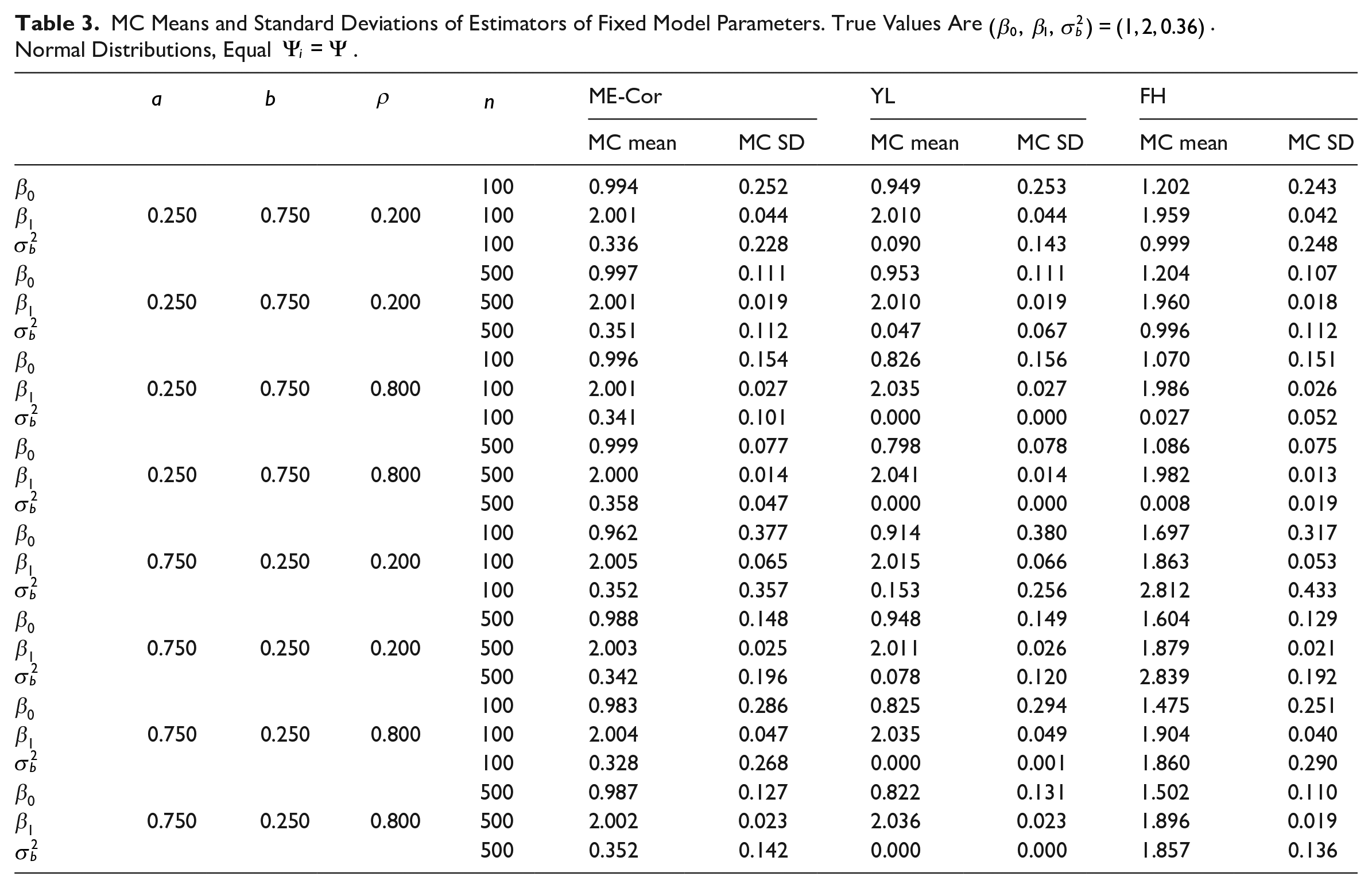
MC Means and Standard Deviations of Estimators of Fixed Model Parameters. True Values Are
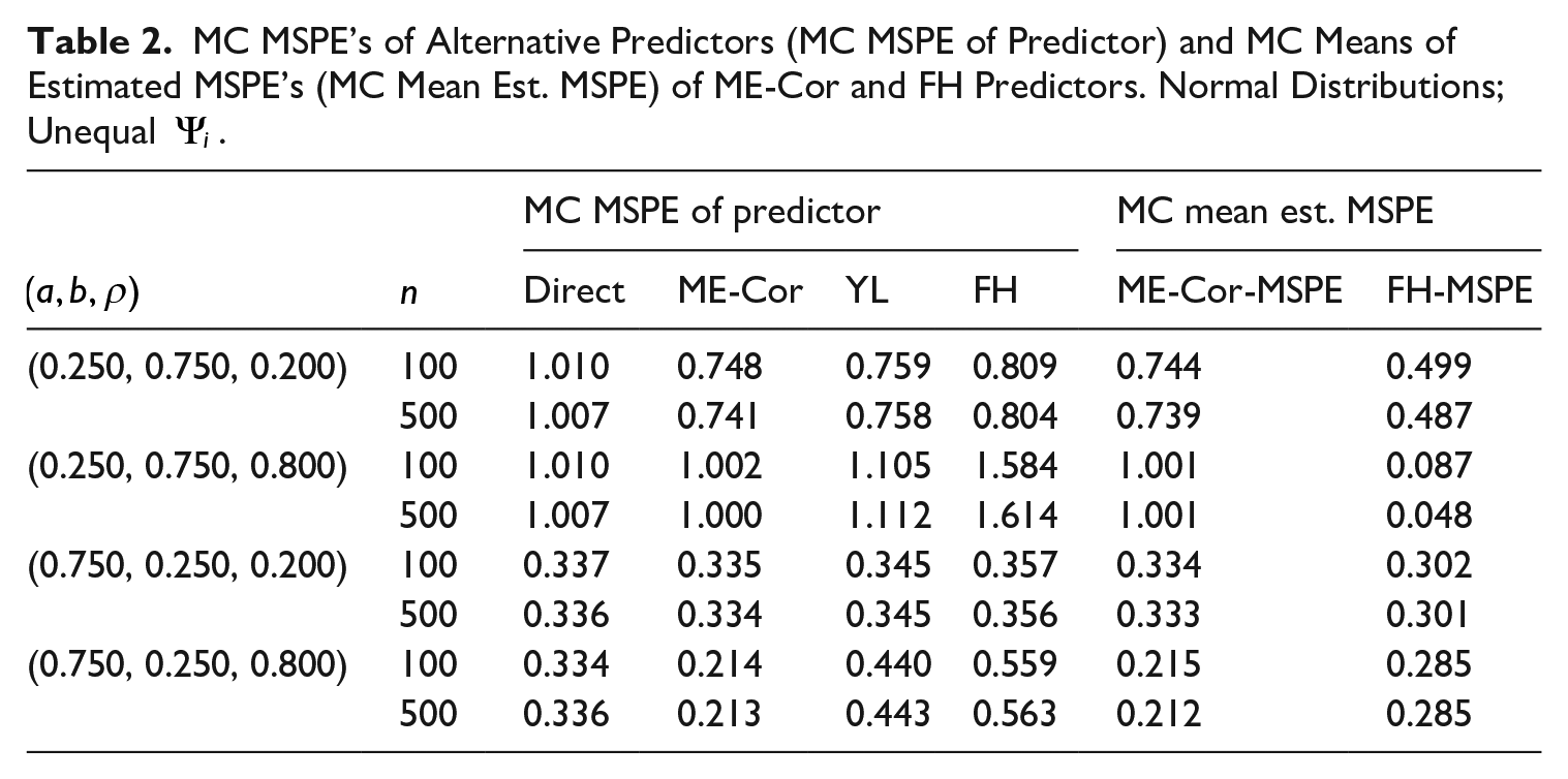
MC MSPE’s of Alternative Predictors (MC MSPE of Predictor) and MC Means of Estimated MSPE’s (MC Mean Est. MSPE) of ME-Cor and FH Predictors. Normal Distributions; Unequal
The proposed estimator of
The presence of a nontrivial correlation between
The measurement error attenuates the FH estimator of the slope toward zero and leads to a positive bias in the estimator of the intercept. The FH estimator of
Table 2 summarizes the empirical properties of the alternative predictors and MSPE estimators. The columns under the heading “MC MSPE of Predictor” contain the average MC MSPE’s of the alternative predictors, where the average is across areas. The columns under the heading “MC Mean Est. MSPE” contain the average MC means of the MSPE estimators for the ME-Cor and FH procedures. The column labeled “Direct” indicates the average MC MSPE of the direct estimator,
The YL predictor is superior to the FH predictor but inferior to the ME-Cor predictor. For all but the configuration with
The properties of the FH predictor depend on the structure of
The efficiency of the FH predictor relative to the direct estimator is best when
An important implication of measurement error is that the Fay-Herriot MSPE estimator (FH-MSPE) has a severe negative bias for the MSPE of the Fay-Herriot predictor (FH). When
The ME-Cor predictor has smaller MC MSPE than the alternatives considered for all configurations. When
The proposed MSPE estimator (ME-Cor-MSPE) is a good approximation for the MSPE of the ME-Cor predictor (ME-Cor). For each configuration, the average MC mean of the estimated MSPE for the ME-Cor predictor (ME-Cor-MSPE) is close to the average MC MSPE of the ME-Cor predictor (ME-Cor). The simulation results support the predictor and MSPE estimator proposed in Section 2.
3.2. Normal Distributions, Equal
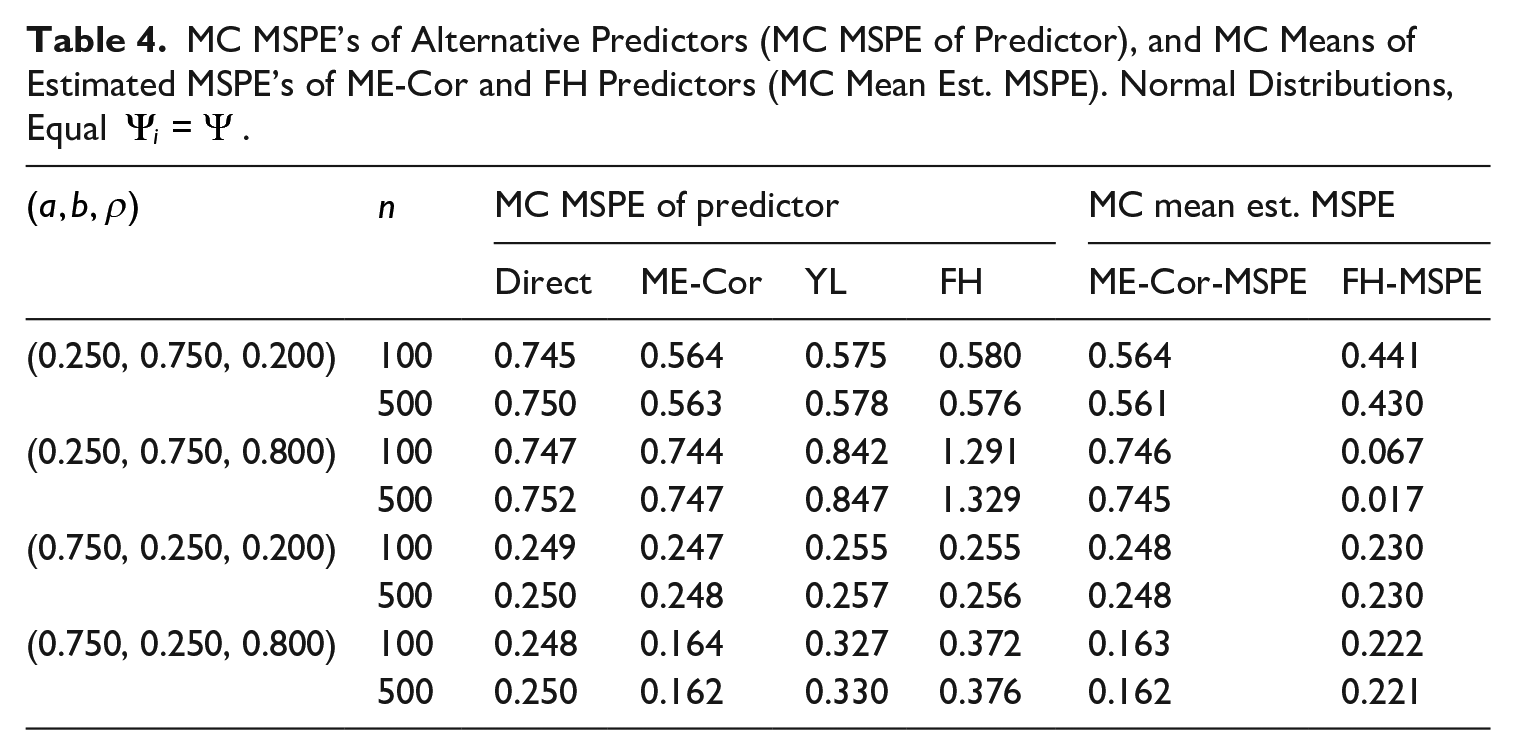
A special case in which the FH predictor retains reasonable properties occurs in the context of the structural model when the measurement error is uncorrelated with the sampling error and when the measurement error variance is constant (Bell et al. 2019). When the measurement error and sampling error are correlated, the naive Fay-Herriot predictor remains inappropriate, even if the measurement error variance is constant. To illustrate this point, we present simulation results with equal
Tables 3 and 4 contain simulation results for
MC Means and Standard Deviations of Estimators of Fixed Model Parameters. True Values Are
MC MSPE’s of Alternative Predictors (MC MSPE of Predictor), and MC Means of Estimated MSPE’s of ME-Cor and FH Predictors (MC Mean Est. MSPE). Normal Distributions, Equal
3.3. Simulations with
Distributions
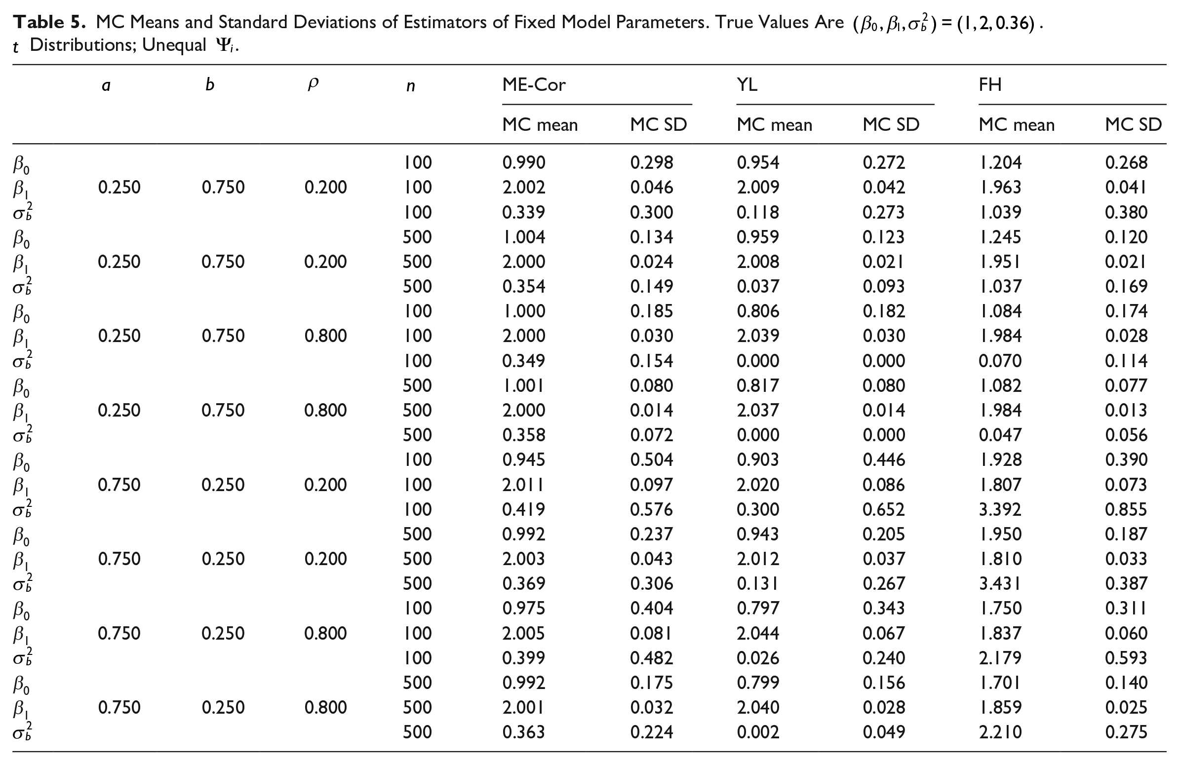
We next simulate data from
The results for the
MC Means and Standard Deviations of Estimators of Fixed Model Parameters. True Values Are
MC MSPE’s of Alternative Predictors (MC MSPE of Predictor), and MC Means of Estimated MSPE’s of ME-Cor and FH Predictors (MC Mean Est. MSPE).
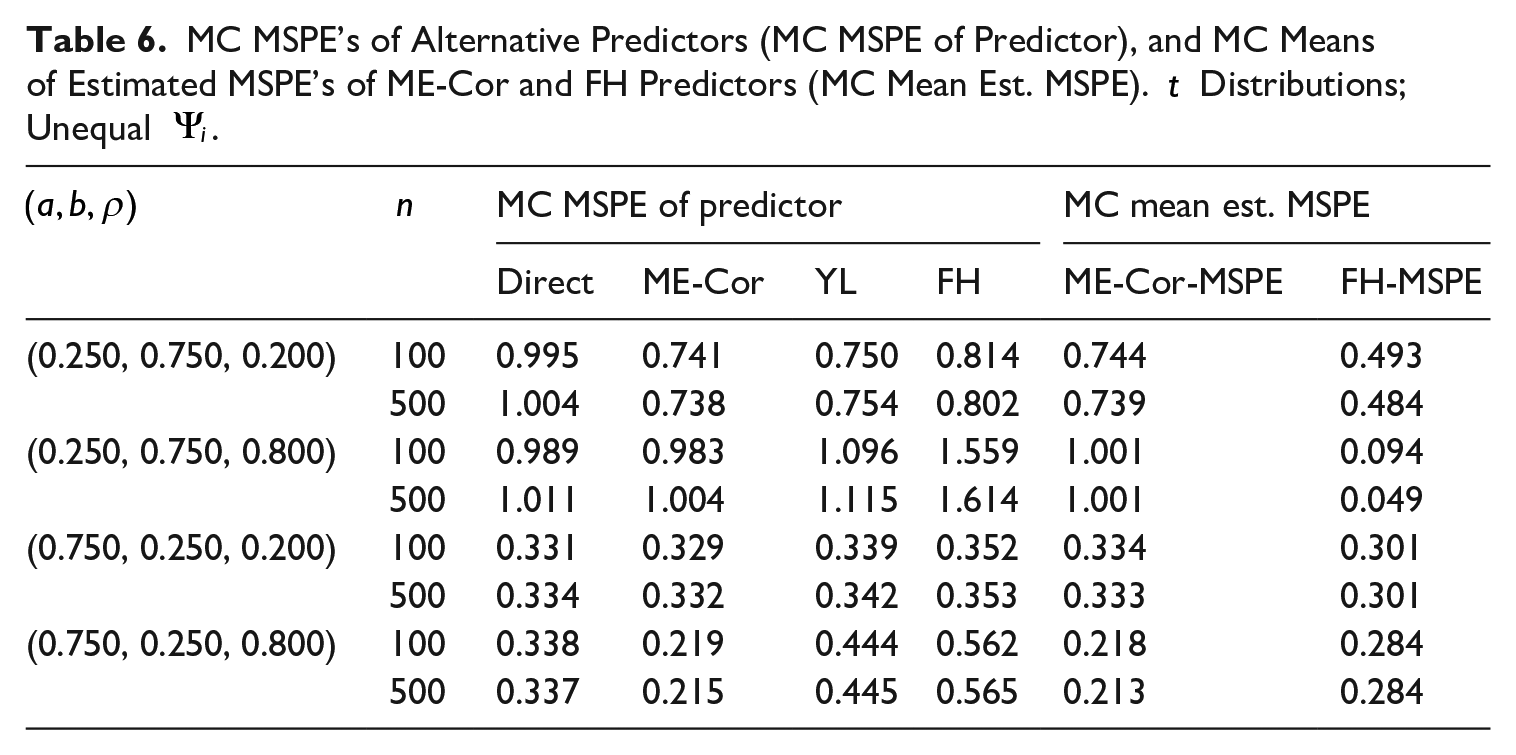
For configurations with
The positive bias of the estimator of
The FH and YL procedures remain inefficient when the data are generated from
3.4. Extended Simulations
We present extended simulation results in the Supplemental Material. First, we use a
These extended configurations allow us to assess the impacts of skewness and absence of fourth moments on the properties of the proposed procedure. The positive bias of the estimator of
We also validate the proposed procedure for a multivariate covariate in the Supplemental Material. We use two covariates, both of which are measured with error. The estimators of the fixed parameters remain nearly unbiased in the presence of a bivariate covariate. The proposed MSPE estimator is also nearly unbiased for the MSPE of the predictor.
4. CEAP Data Analysis
We apply the method proposed in Section 2 to predict mean log sheet and rill erosion in Iowa counties using CEAP data. Iowa has
We connect the context and notation of Section 2 to the CEAP data analysis. Let
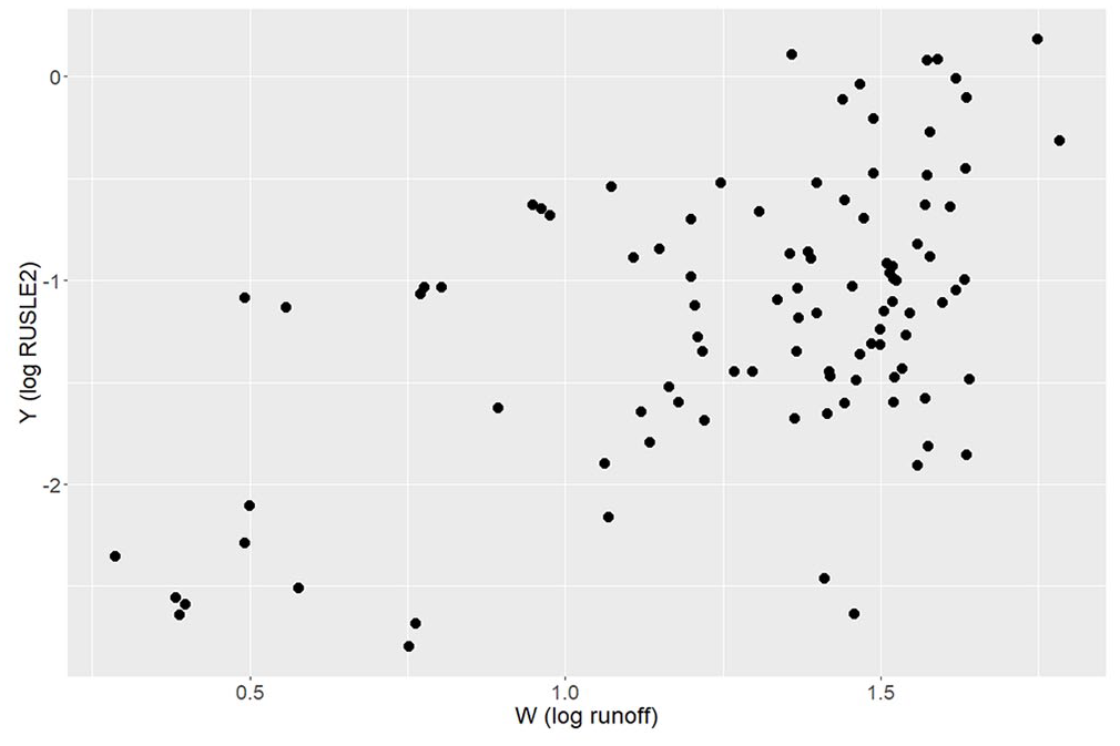
Scatterplot of
The model requires an estimate of
For this analysis, we treat the direct estimator of
We assume that the model (1) holds for
Table 7 contains the estimate of
Estimates of Fixed Model Parameters and Associated Standard Errors for CEAP Data.
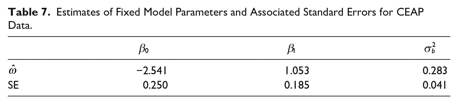
The magnitude of the estimate of each parameter is more than double the corresponding standard error.
For the CEAP data analysis, several of the estimated MSPE’s are negative. We therefore apply a lower bound (LB) to the estimated MSPE for the CEAP analysis. We define the MSPE estimator for the CEAP study by

where
Figure 2 contains a scatterplot illuminating the relationship between the efficiency gain from prediction and the components of the design covariance matrix. The
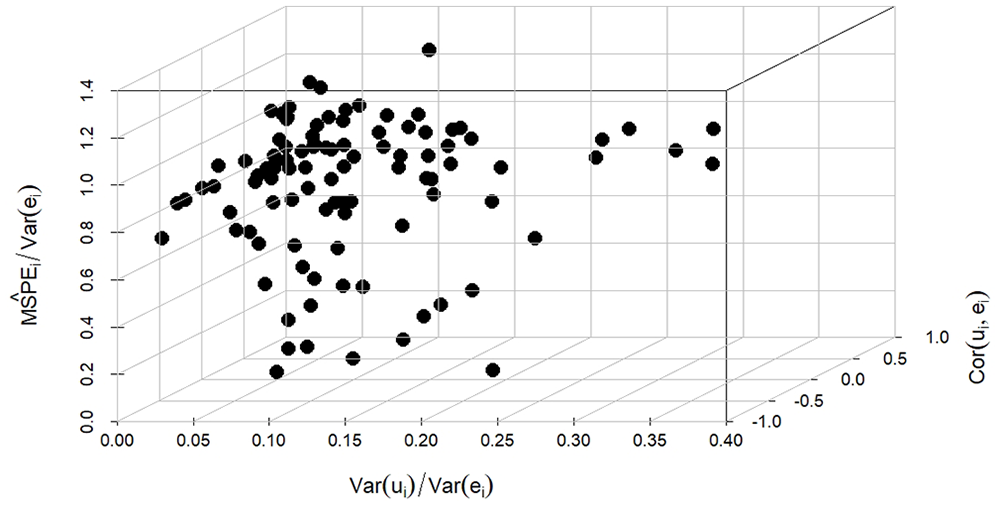
Three-dimensional scatterplot with
From Figure 2, it is apparent that an efficiency gain is attained for most counties. The relative mean square prediction errors range from 0.056 to 1.222, and the average is 0.781. The efficiency gains are often pronounced when
The left panel of Figure 3 contains a scatterplot of the predictors on the vertical axis against the direct estimators on the horizontal axis. The line in the plot is the 45-degree line through the origin. Small area prediction has the expected shrinkage effect. Prediction increases direct estimators that are unusually low and decreases direct estimators that are unusually high.
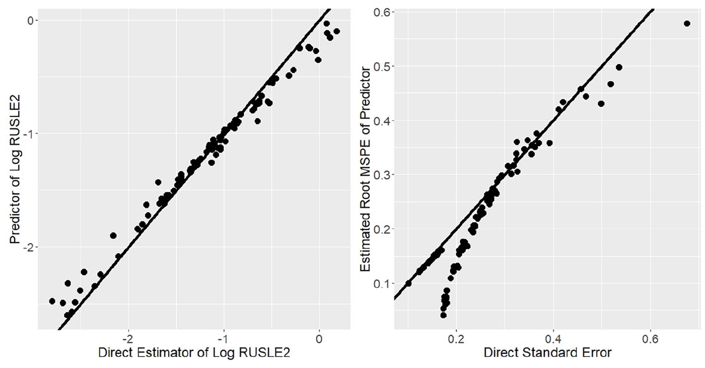
Left: Scatterplot of predictors against direct estimators. Right: Scatterplot of root MSPE estimators against square roots of estimated variances of direct estimators.
The right panel of Figure 3 contains a plot of the square roots of the mean square prediction errors against the standard errors of the direct estimators. The line is again the 45-degree line through the origin. For most counties, prediction renders an efficiency gain relative to the direct estimator. The reduction in MSPE from prediction is often substantial. When the MSPE exceeds the estimated variance of the direct estimator, the estimated loss of efficiency is minimal.
5. Discussion
We conduct an extensive study of the properties of a small area predictor that recognizes a correlation between the measurement error in the covariate and the sampling error in the response. The simulation studies illustrate the dangers of naively applying the Fay-Herriot predictor when the covariate and response are estimators from the same survey. The Fay-Herriot predictor can be less efficient than the direct estimator, and the corresponding MSPE estimator can have a severe negative bias for the MSPE of the predictor. The problems with the Fay-Herriot predictor persist even when
The proposed predictor rectifies the problems with the Fay-Herriot predictor and is more efficient than other alternatives considered in the simulations. In both the simulations and the data analysis, the efficiency of the proposed method relative to the direct estimator depends on the nature of
Supplemental Material
sj-pdf-1-jof-10.1177_0282423X241240835 – Supplemental material for An Application of a Small Area Procedure with Correlation Between Measurement Error and Sampling Error to the Conservation Effects Assessment Project
Supplemental material, sj-pdf-1-jof-10.1177_0282423X241240835 for An Application of a Small Area Procedure with Correlation Between Measurement Error and Sampling Error to the Conservation Effects Assessment Project by Emily Berg and Sepideh Mosaferi in Journal of Official Statistics
Footnotes
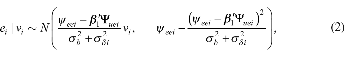
Appendix A: Derivation of Conditional Distribution of ei Given vi
We provide further detail on the derivation of the distribution of
where we have used the definition of
and
Appendix B: Statistical Properties of Estimators and Predictors
We state and prove Theorems 1 and 2 for the case of univariate
We denote the univariate slope and estimator of
Then,
where
Then
Appendix C: Direct Estimators for CEAP
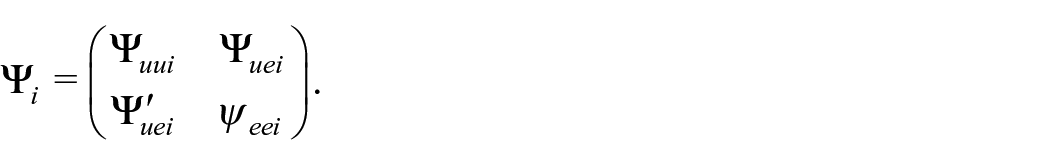
We explain how we estimate Ψi for the CEAP data. We let
We let
where
Funding
The author(s) disclosed receipt of the following financial support for the research, authorship, and/or publication of this article: Emily Berg was partially supported by the U.S. Department of Agriculture’s National Resources Inventory, Cooperative Agreement NR203A750023C006, Great Rivers CESU 68-3A75-18-504.
Supplemental Material
Supplemental material for this article is available online.
Received: October 2021
Accepted: November 2022
References
Supplementary Material
Please find the following supplemental material available below.
For Open Access articles published under a Creative Commons License, all supplemental material carries the same license as the article it is associated with.
For non-Open Access articles published, all supplemental material carries a non-exclusive license, and permission requests for re-use of supplemental material or any part of supplemental material shall be sent directly to the copyright owner as specified in the copyright notice associated with the article.