Fault-tolerant decentralized multi-sensor link velocity and acceleration estimation for elastic-joint robots

Abstract

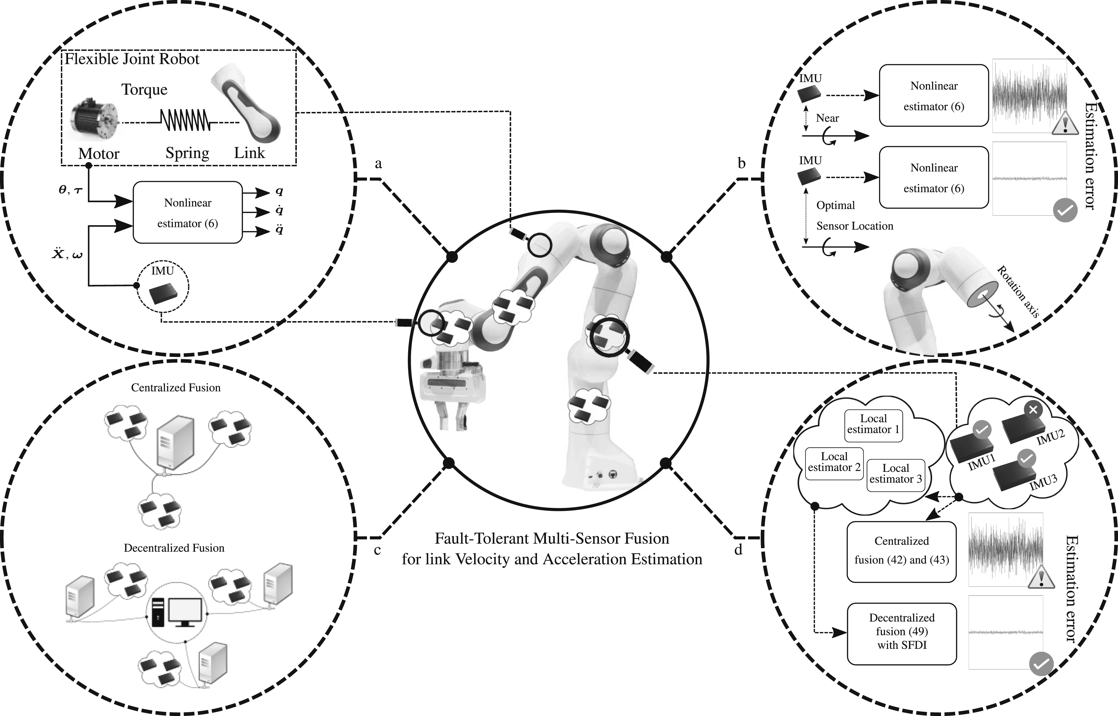
In robot manipulators position sensing has been well established as a core kinematics measurement, while velocity is typically numerically deduced from it via differentiation. However, various algorithms, whether they be control, collision monitoring and detection, friction compensation, learning-based methods, or model identification, all would highly benefit from accurate and high-bandwidth link-side velocity and acceleration information. In this work, we address the problem of decentralized multi-sensor fusion for estimating high-accuracy and high-bandwidth link-side velocity and acceleration for both rigid-body as well as flexible-joint robot manipulators. This is done via fusing the joint torque and motor position measurements with inertial measurement units (IMUs) mounted on the robot structure. Moreover, we discuss how to optimally distribute these IMUs along the robot structure. One goal is to maximize signal-to-noise ratio in the sense of Fisher and consequently allow for more accurate estimation results. A secondary goal may be to increase the probability of detection of unwanted and unpredictable collisions. Furthermore, since the proposed setup relies on different sensor types—which can be further exploited—a practical yet simple sensor failure detection and isolation scheme is introduced. We evaluate our claims and methods in simulations and experiments based on a state-of-the-art 7 degrees of freedom (DoF) manipulator.

Introduction and state of the art

Over the last decades, robot manipulators have evolved from expensive, bulky structures to affordable, lightweight mechatronic systems. At the same time, control algorithms, as well as safety policies, have been adapted significantly to suit the market demands, not only for industrial robots but also for service and domestic applications. In particular, these algorithms aim at optimally fulfilling the respective tasks while ensuring human safety (Stilli et al., 2017; Sangiovanni et al., 2018). For achieving this ambitious goal, inherently safer design and rich sensory perception have become vital ingredients.

Similar to other complex engineered systems, robot manipulators acquire information about themselves and their surroundings via various proprioceptive and exteroceptive sensors. Next to motor torque τ _m, link-side joint torque τ _J, and link position q , it is highly desirable to directly measure link-side joint velocity $\dot{\mathit{q}}$ and joint acceleration $\ddot{\mathit{q}}$ . In principle, they are needed in numerous algorithms, ranging from robust motion control (Sage et al., 1999) to friction compensation (Canudas De Wit et al., 1991) and collision monitoring (Haddadin et al., 2017). However, in real implementations, acceleration is typically replaced by (i) lower-accuracy, low-bandwidth estimations, (ii) second numerical differentiation from position sensing, or (iii) avoided entirely, as second numerical differentiation of quantized signals results in non-practical signal-to-noise ratios (Choi, 2009). Link velocity $\dot{\mathit{q}}$ , on the other hand, can still be obtained by numerical differentiation of link position and suitable low-pass filtering. However, this approach is obviously limited in accuracy, and only limited bandwidth can be achieved (Baradaran Birjandi et al., 2019). These limitations have led to various compromise solutions instead of aiming for the theoretical ideal. Consider, for example, the widely used generalized momentum observer for real-time collision monitoring (De Luca and Mattone, 2005). It bypasses the necessity of link acceleration $\ddot{\mathit{q}}$ at the cost of lower detection bandwidth. Another well-known example is model or load inertia parameter identification. For lag-free filtering, these algorithms are generally employed offline (Atkeson et al., 1986; Kozlowski, 2012).

However, only recently we have shown that with the help of IMUs, which have become miniaturized and affordable over the last ten years, one can solve this problem in principle and overcome current limitations. Fusing IMU information consisting of a triaxial accelerometer, a triaxial gyroscope, and a magnetometer with other well-established measurements in robot manipulators, namely, position q and joint torque τ _J, will increase not only the estimation bandwidth and accuracy but also numerical stability and overall system fault tolerance (Baradaran Birjandi et al., 2019; Baradaran Birjandi et al., 2020).

This advancement has become possible due to the vast optimization in size, accuracy, and power specifications of micro-electromechanical systems such as IMUs in general (Perlmutter and Breit, 2016). These sensors paved the way from navigation systems in airplanes and ships to significantly smaller devices such as smartphones. These sensors have proven to be useful in highly dynamic scenarios as well (see, e.g., Schepers et al., 2018; Stefanov et al., 2020). In robot manipulators, however, IMUs are utilized—if at all—for online calibration (Du and Zhang, 2013; Zhang et al., 2015) or joint orientation estimation (Wieser et al., 2011). In fact, and to the best of the authors’ knowledge, the integration of IMUs for accurate link velocity and acceleration estimation in robot manipulators with their highly nonlinear and coupled dynamics has only been exploited marginally so far. Presumably, this is because manipulators were originally not equipped with IMUs, and various mechatronic constraints, such as integrating IMUs into the low-level control structure, would have to be solved. Also, finding the best location for installing IMUs within the robot structure has not yet been addressed. One of the rare examples using accelerometers for estimating rigid manipulator joint velocity and acceleration can be found in McLean et al. (2015). There, built-in motor encoders are fused with external accelerometers to estimate relative joint position, velocity, and acceleration components. The main limitation of this method is that it requires at least four accelerometers per link. Our previous works (Baradaran Birjandi et al., 2019; Baradaran Birjandi et al., 2020; Baradaran Birjandi et al., 2023a,b), on the other hand, introduced a new method for estimating link velocity and acceleration in rigid robots with only a single IMU necessary per link. Furthermore, our approach does not require the Lagrangian dynamics model and is computationally very lightweight. Finally, the motion dynamics model, used in our proposed estimator, can be used to estimate robot motions over wide frequency ranges. This work, in fact, continues the seminal contributions of De Luca et al. (2007), who first fused accelerometers—nowadays integrated within IMUs—with internal robot measurements to estimate link velocity and acceleration. Recent research, such as the works of Fennel et al. (2022), also explored similar methodologies, demonstrating the potential of IMUs in enhancing kinematic state estimation for robotic systems. In this manuscript, we compare our proposed method against these earlier approaches, establishing the advancements made in our technique.

In this paper, we base on this previous work and generalize it toward reliable and fault-resilient estimation of link velocity and acceleration in rigid-body as well as flexible-joint robot manipulators by fusing multiple redundant IMUs with proprioceptive sensory systems, as detailed next.

Contribution

Over the past few years, IMUs have become an affordable, highly integrated and user-friendly technology, allowing us to reconsider the way the kinematic states $(\mathit{q},\dot{\mathit{q}},\ddot{\mathit{q}})$ of a robot can be acquired: We show that multiple redundant IMUs installed per link can be fused with proprioceptive sensors for failure-resilient, robust and accurate link-side velocity and acceleration estimation in flexible-joint robot manipulators. Specifically, the following contributions are made (see Figure 1).

First, we generalize our previous link velocity and acceleration estimation scheme for rigid robots (Baradaran Birjandi et al., 2019; Baradaran Birjandi et al., 2020) to flexible-joint robots. This makes our method available to modern collaborative and tactile robots with their lightweight structure and elastic joints due to harmonic drives, shaft windup, and bearing deformation.

Second, we analyze the optimal placement of IMUs in the link structure to optimize their signal-to-noise ratio (SNR) in the sense of the Fisher information matrix (FIM). Consequently, with this, the effect of an IMU on link-side variable estimation can be quantitatively investigated and, therefore, optimized. This may greatly improve applications such as IMU-based collision monitoring, where the slightest and most distal collisions on the corresponding link are to be detected.

Third, we elaborate on how multiple IMU sensors per link may be fused via centralized or decentralized architectures and evaluate their respective performance.

Fourth, the proposed proprioceptive sensor system, including motor position, joint torque, and multiple IMUs per joint/link unit, is further enhanced by a simple yet fast and powerful sensor failure detection and isolation (SFDI) algorithm that allows for robust state estimation despite sensor failures.

Figure 1.

Summary of contributions: (a) Estimating link-side velocity and acceleration by fusing IMUs installed on the robot links with proprioceptive sensing. (b) Placing IMUs on the link surface for maximum estimation accuracy. (c) Designing different architectures for multiple-IMU fusion. (d) Tackling sensor failures in the setup.

According to our results, the proposed method estimates link velocity with accuracy comparable to the state of the art and achieves up to threefold higher accuracy in link acceleration estimation.

Background

The multidisciplinary research challenge tackled in this paper requires methods from several fields, summarized in the following.

Fisher information matrix

Given an observable random variable with an unknown parameter, the Fisher information matrix (FIM) quantifies how much information the random variable provides about the unknown parameter over a certain number of observations. If—given the parameter that may be a system state—the likelihood function of the random variable is independent of the parameter, the corresponding FIM will be zero, that is, the random variable carries no information about the parameter. Conversely, the more sensitive the likelihood function is to changes in the parameter, the larger the FIM becomes, allowing the parameter to be estimated with available observations (Ghosh et al., 2007). Therefore, FIM is defined as the variance (or sensitivity) of the score function, which is associated with the estimation problem (Schervish, 2012). FIM may, for example, be used to define a convex objective function, which models the sensor placement problem in engineering systems (Xygkis et al., 2016), making it particularly useful for multi-sensor systems.

Sensor fusion

Multi-sensor fusion in model-based predictions is a means to increase state estimation reliability and accuracy (Julier and Uhlmann, 2017; Luo et al., 2002). Model-based multi-sensor fusion finds many applications in civil and military applications. Guidance for autonomous vehicles, remote sensing, and battlefield surveillance are examples of military domains (Julier and Uhlmann, 2017). Robotics, inspection and maintenance of manufacturing processes, and health and environmental monitoring are well-known civilian applications (Luo et al., 2002). Generally, sensor fusion techniques are categorized into centralized and distributed (or decentralized) methods. Table 1 summarizes the pros and cons of each fusion architecture.

Table 1.

Comparison centralized versus decentralized architecture (Julier and Uhlmann, 2017; Bakr and Lee, 2017).

Architecture	Advantage	Disadvantage
Central	Optimal estimation for linear systems	High communication bandwidth
		No failure handling
	Fewer hardware components	Requirement for powerful central unit
		Inflexible architecture
Decentral	Low communication bandwidth	Providing optimal estimation can be challenging
	Cheaper hardware
	Flexible architecture	More hardware components
	Sensor failure handling

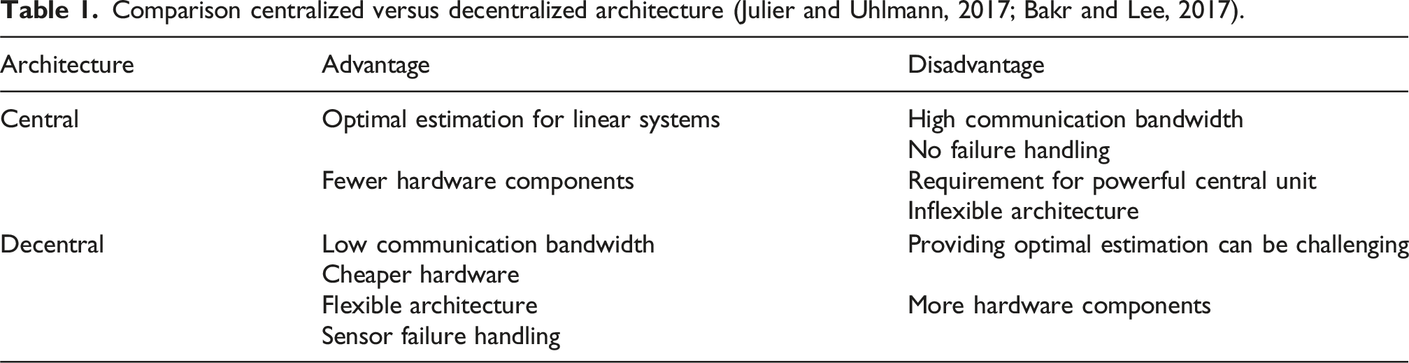
In the centralized fusion architecture (Willner et al., 1976), which is theoretically an estimation problem with distributed data (Li et al., 2003), all sensor data are sent to a central unit, where they are (pre-)processed and fused. In linear systems with zero-mean additive noise, centralized fusion is known to provide the optimal solution. However, this also comes at the cost of possibly large computational loads on the central unit, a relatively inflexible architecture, lack of robustness, and high communication bandwidth requirements (Julier and Uhlmann, 2017; Bakr and Lee, 2017). Another problem with centralized fusion is that its observer gains are computed at the central estimator, leaving measurement failures undetected and causing estimation divergence.

In the decentralized sensor fusion architecture, the local estimators/observers are distributed over the system and send their respective state estimates to a central unit (Bakr and Lee, 2017). However, providing the optimal estimation in the decentralized architectures has been a challenge over the past decades. In Sun and Deng (2004), the optimal multi-sensor decentralized fusion criteria for linear systems with correlated noise were developed. The underlying idea is to weigh each local estimator with optimal coefficients obtained by minimizing the overall estimation error covariance in the Kalman filter. However, a significant difficulty in this approach is the computation of cross-covariance matrices between two local estimators, which is generally expensive. To overcome computational complexities as well as other issues related to decentralized Bayesian estimation, such as the Kalman filter, the concept of covariance intersection (CI) was initially introduced in Julier and Uhlmann (1997). Several studies have shown that CI provides an upper bound on all possible estimation error covariance matrices regarding minimum mean-squared error (Noack et al., 2017). Still, although optimal estimation is not generally assured in decentralized fusion, it does not suffer from the major disadvantages of centralized architectures. Moreover, sensor faults may be handled more efficiently (Sun and Deng, 2004).

Sensor failure detection and isolation

In complex systems with multiple sensors, ensuring the reliability of measurements and the early detection of faults becomes crucial for maintaining system performance and safety. Fusing various sensor types, including redundant sensor configurations, makes sensor fault detection and isolation very relevant. Fault detection falls into four categories: hardware redundancy schemes, signal processing-based approaches, plausibility tests, and analytical/software redundancy algorithms (Ding, 2008). Each class has pros and cons, which are not the focus of this work. We, however, target analytical redundancy schemes, which are relatively young (Ding, 2008). Several analytical redundancy algorithms exist, such as observers (Wang et al., 2017), parity space check (Jin and Zhang, 1999), or the analysis of the innovation sequence in Kalman filtering (Mehra and Peschon, 1971). Due to our system specifications, we focus on observer-based methods. The residual, the difference between measurements and estimations, is constantly monitored in most fault-detection methods, including observer-based algorithms. Failures are detected and isolated to provide high reliability with minimum delay (Martinez-Guerra and Mata-Machuca, 2016).

The remainder of this article is organized as follows. The theoretical framework for solving the addressed problems for the considered system class is developed in Section State Estimation. The theory is subsequently elaborated in simulations and experiments in the subsequent Section Evaluation. Finally, the paper concludes with concluding remarks in Section Conclusion. The summary and logical flow of topics discussed in this paper are depicted in Figure 2.

Figure 2.

Summary of the topics covered in this manuscript.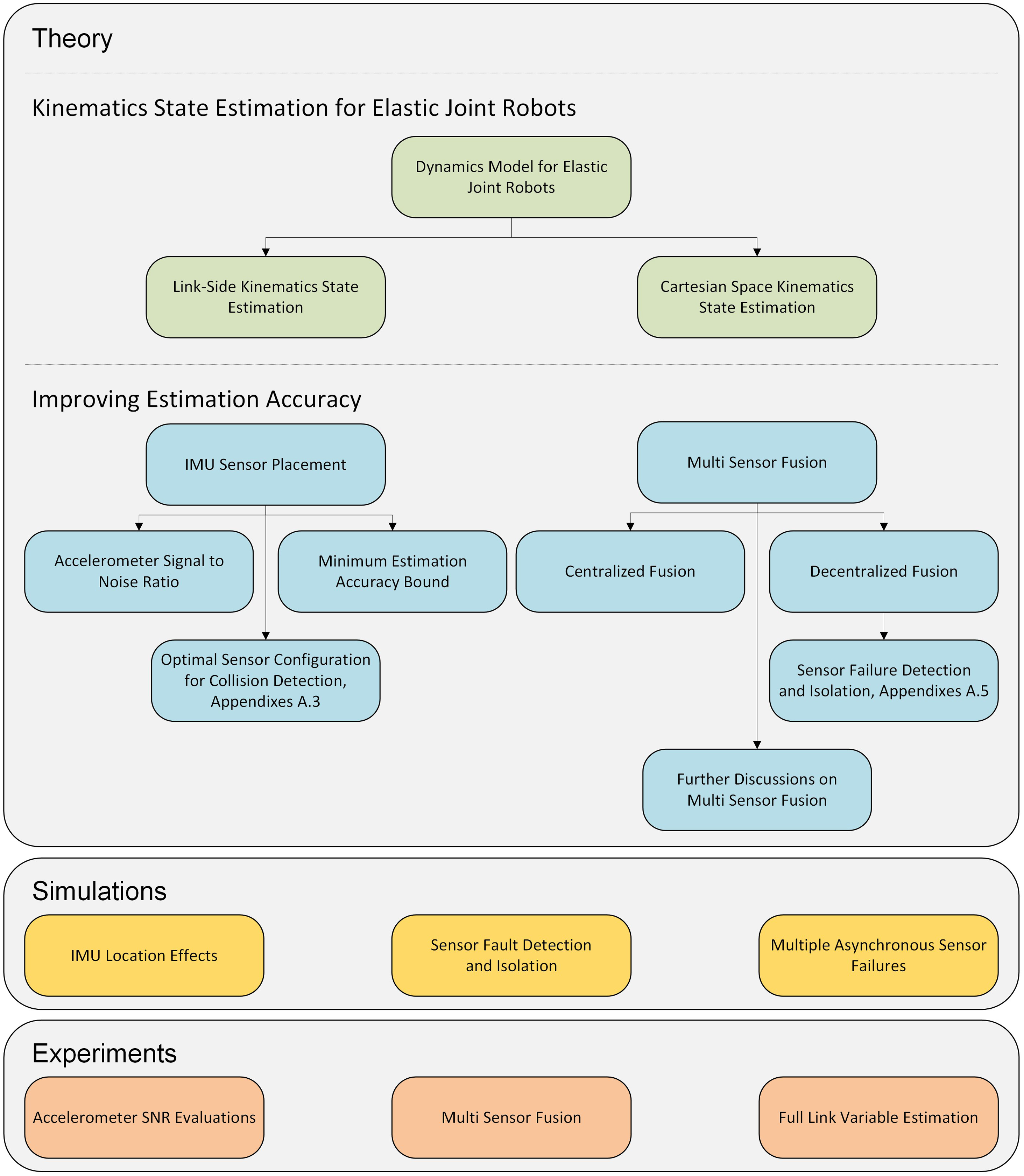

State estimation

Elastic-joint robot

Consider the standard reduced dynamics model of a robot manipulator with $\mathrm{n}$ elastic joints (Spong, 1987)

$\mathit{M}(\mathit{q})\ddot{\mathit{q}}+\mathit{C}(\mathit{q},\dot{\mathit{q}})\dot{\mathit{q}}+\mathit{g}(\mathit{q})={\mathit{\tau }}_{\text{J}}+{\mathit{D}}_{\text{J}}{\mathit{K}}_{\text{J}}^{-1}{\dot{\mathit{\tau }}}_{\text{J}}$

(1)

$\mathit{B}\ddot{\mathit{\theta }}+{\mathit{\tau }}_{\text{J}}+{\mathit{D}}_{\text{J}}{\mathit{K}}_{\text{J}}^{-1}{\dot{\mathit{\tau }}}_{\text{J}}={\mathit{\tau }}_{\text{m}}-{\mathit{\tau }}_{\text{f}}$

(2)

${\mathit{\tau }}_{\text{J}}={\mathit{K}}_{\text{J}}(\mathit{\theta }-\mathit{q}),$

(3)

where $\mathit{\theta }\in {\mathbb{R}}^{\text{n}}$ denotes the motor position and $\mathit{q},\dot{\mathit{q}},\ddot{\mathit{q}}\in {\mathbb{R}}^{\text{n}}$ the link-side position, velocity, and acceleration, respectively. $\mathit{M}(\mathit{q})\in {\mathbb{R}}^{\text{n}\times \mathrm{n}}$ is the symmetric and positive definite inertia matrix, $\mathit{C}(\mathit{q},\dot{\mathit{q}})\dot{\mathit{q}}\in {\mathbb{R}}^{\text{n}}$ the centrifugal and Coriolis vector, $\mathit{g}(\mathit{q})\in {\mathbb{R}}^n$ the gravity vector, ${\mathit{\tau }}_{\text{J}}\in {\mathbb{R}}^{\text{n}}$ the elastic joint torque, ${\mathit{\tau }}_{\text{m}}\in {\mathbb{R}}^{\text{n}}$ the active motor torque, ${\mathit{\tau }}_{\text{f}}\in {\mathbb{R}}^{\text{n}}$ the friction torque, ${\mathit{D}}_{\text{J}}=\text{diag}\{D_{J,i}\}\in {\mathbb{R}}^{\text{n}\times \mathrm{n}}$ the diagonal positive semi-definite joint damping matrix, ${\mathit{K}}_{\text{J}}=\text{diag}\{K_{\text{J,i}}\}\in {\mathbb{R}}^{\text{n}\times \mathrm{n}}$ the diagonal positive definite joint stiffness matrix, and $\mathit{B}=\text{diag}\{{\mathit{B}}_{\text{i}}\}\in {\mathbb{R}}^{\text{n}\times \mathrm{n}}$ the diagonal positive definite motor inertia matrix. Note that motor-side position $\mathit{\theta }$ as well as the elastic joint torque ${\mathit{\tau }}_{\text{J}}\in {\mathbb{R}}^{\text{n}}$ are assumed to be measurable in this setup, as this has become state-of-the-art in particular in recent collaborative and tactile robots (Seok et al., 2020).

Link velocity and acceleration estimation

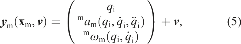
In elastic-joint manipulators, motor- and link-side positions are linearly coupled according to equation (3). However, note that only motor encoders and joint torques are available measurements. In contrast to the current state of the art, we assume that every link is equipped with at least one IMU, which in turn consists of a 3-axis accelerometer and a 3-axis gyroscope. In order to model the full elastic-joint manipulator link state, we therefore propose the following realistic dynamics model with a constant-jerk assumption ¹ :

$\begin{array}{ll}\hfill & \frac{\text{d}}{\text{d}t}{\mathbf{x}}_{\text{m}}={\mathit{f}}_{\text{m}}({\mathbf{x}}_{\text{m}},\mathit{w})=\left(\begin{array}{cccc}\hfill 0\hfill & \hfill 1\hfill & \hfill 0\hfill & \hfill 0\hfill \\ \hfill 0\hfill & \hfill 0\hfill & \hfill 1\hfill & \hfill 0\hfill \\ \hfill 0\hfill & \hfill 0\hfill & \hfill 0\hfill & \hfill 1\hfill \\ \hfill 0\hfill & \hfill 0\hfill & \hfill 0\hfill & \hfill 0\hfill \end{array}\right){\mathbf{x}}_{\text{m}}+\mathit{w}\hfill \\ \hfill & {\mathit{y}}_{\text{m}}({\mathbf{x}}_{\text{m}},\mathit{v},\mathit{\zeta }(t))=\left(\begin{array}{c}\hfill q_{\text{i}}={\theta }_{\text{i}}-{\tau }_{\text{J,i}}/K_{\text{J,i}}\hfill \\ \hfill {}^{\text{m}}\mathit{a}_{\text{m}}(q_{\text{i}},{\dot{q}}_{\text{i}},{\ddot{q}}_{\text{i}})\hfill \\ \hfill {}^{\text{m}}\mathit{\omega }_{\text{m}}(q_{\text{i}},{\dot{q}}_{\text{i}})\hfill \end{array}\right)+\mathit{v}+\mathit{\zeta }(t),\hfill \end{array}$

(4)

where m indicates the estimator index and i that of the links, with indices $\mathrm{m}$ and $\mathrm{i}$ being uncorrelated. In fact, more than one estimator might be estimating the i-th link variables if more than one IMU is installed on the corresponding link. Herein, ${\mathbf{x}}_{\text{m}}={[q_{\text{i}}{\dot{q}}_{\text{i}}{\ddot{q}}_{\text{i}}{\stackrel{⃛}{q}}_{\text{i}}]}^T\in {\mathbb{R}}^4$ denotes the system state with q_i, ${\dot{q}}_{\text{i}}$ , ${\ddot{q}}_{\text{i}}$ , and ${\stackrel{⃛}{q}}_{\text{i}}\in \mathbb{R}$ being the link position, velocity, acceleration, and jerk of the i-th link and m-th estimator. Moreover, ${\mathit{f}}_{\text{m}}(\cdot ):{\mathbb{R}}^4\times {\mathbb{R}}^4\to {\mathbb{R}}^4$ represents the m-th state transition function. The corresponding measurement function ${\mathit{y}}_{\text{m}}(\cdot ):{\mathbb{R}}^4\times {\mathbb{R}}^7\to {\mathbb{R}}^7$ includes the Cartesian acceleration ${}^{\text{m}}\mathit{a}_{\text{m}}(\cdot ):\mathbb{R}\times \mathbb{R}\times \mathbb{R}\to {\mathbb{R}}^3$ and angular velocity ${}^{\text{m}}\mathit{\omega }_{\text{m}}(\cdot ):\mathbb{R}\times \mathbb{R}\to {\mathbb{R}}^3$ at the location of sensor m expressed in sensor frame {m}. With the help of equation (3) and the computed/estimated joint stiffness matrix K _J, the i-th link position q_i is expressed in terms of the measured quantities θ_i and τ_J,i ² . This step extends our previous idealized work on rigid-body manipulators (Baradaran Birjandi et al., 2019; Baradaran Birjandi et al., 2020) to flexible joint robots. For the rigid system, the measurement function was proposed to be

${\mathit{y}}_{\text{m}}({\mathbf{x}}_{\text{m}},\mathit{v})=\left(\begin{array}{c}\hfill q_{\text{i}}\hfill \\ \hfill {}^{\text{m}}\mathit{a}_{\text{m}}(q_{\text{i}},{\dot{q}}_{\text{i}},{\ddot{q}}_{\text{i}})\hfill \\ \hfill {}^{\text{m}}\mathit{\omega }_{\text{m}}(q_{\text{i}},{\dot{q}}_{\text{i}})\hfill \end{array}\right)+\mathit{v},$

(5)

where the link position is assumed to be directly measured. Moreover, $\mathit{w}\in {\mathbb{R}}^4$ and $\mathit{v}\in {\mathbb{R}}^7$ are zero-mean white Gaussian process and measurement noise with known covariance matrices, respectively. Finally, $\mathit{\zeta }(t):\mathbb{R}\to {\mathbb{R}}^7$ in equation (4) is the unknown sensor failure vector. Therefore, the estimator model is given by

$\begin{array}{ll}\hfill & \frac{\text{d}}{\text{d}t}{\widehat{\mathbf{x}}}_{\text{m}}={\mathit{f}}_{\text{m}}({\widehat{\mathit{x}}}_{\text{m}},\widehat{\mathit{w}})=\left(\begin{array}{cccc}\hfill 0\hfill & \hfill 1\hfill & \hfill 0\hfill & \hfill 0\hfill \\ \hfill 0\hfill & \hfill 0\hfill & \hfill 1\hfill & \hfill 0\hfill \\ \hfill 0\hfill & \hfill 0\hfill & \hfill 0\hfill & \hfill 1\hfill \\ \hfill 0\hfill & \hfill 0\hfill & \hfill 0\hfill & \hfill 0\hfill \end{array}\right){\widehat{\mathbf{x}}}_{\text{m}}+\widehat{\mathit{w}}\hfill \\ \hfill & {\widehat{\mathit{y}}}_{\text{m}}({\widehat{\mathbf{x}}}_{\text{m}},\widehat{\mathit{v}})=\left(\begin{array}{c}\hfill {\widehat{\mathbf{x}}}_{\text{m}}(1)={\widehat{q}}_{\text{i}}\hfill \\ \hfill {}^{\text{m}}\widehat{\mathit{a}}_{\text{m}}({\widehat{q}}_{\text{i}},{\widehat{\dot{q}}}_{\text{i}},{\widehat{\ddot{q}}}_{\text{i}})\hfill \\ \hfill {}^{\text{m}}\widehat{\mathit{\omega }}_{\text{m}}({\widehat{q}}_{\text{i}},{\widehat{\dot{q}}}_{\text{i}})\hfill \end{array}\right)+\widehat{\mathit{v}}.\hfill \end{array}$

(6)

Here, the hat symbol $(\widehat{\cdot })$ indicates that the real values are replaced by the estimates. Figure 3 depicts the estimator block diagram with all relevant measurements. In this section, we do not account for sensor failures (i.e., ζ = 0 ). Besides the minor difference in the measurement function between rigid-body and flexible-joint manipulators, dynamics model equation (6) has proven to be computationally lightweight and easy to implement with high bandwidth thanks to various sensor fusion strategies (Baradaran Birjandi and Haddadin, 2020).

Figure 3.

Block diagram of estimator equation (6) for flexible-joint robot manipulators.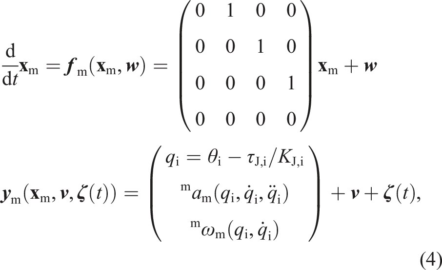

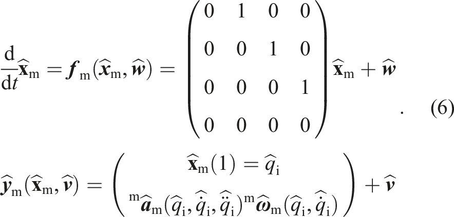
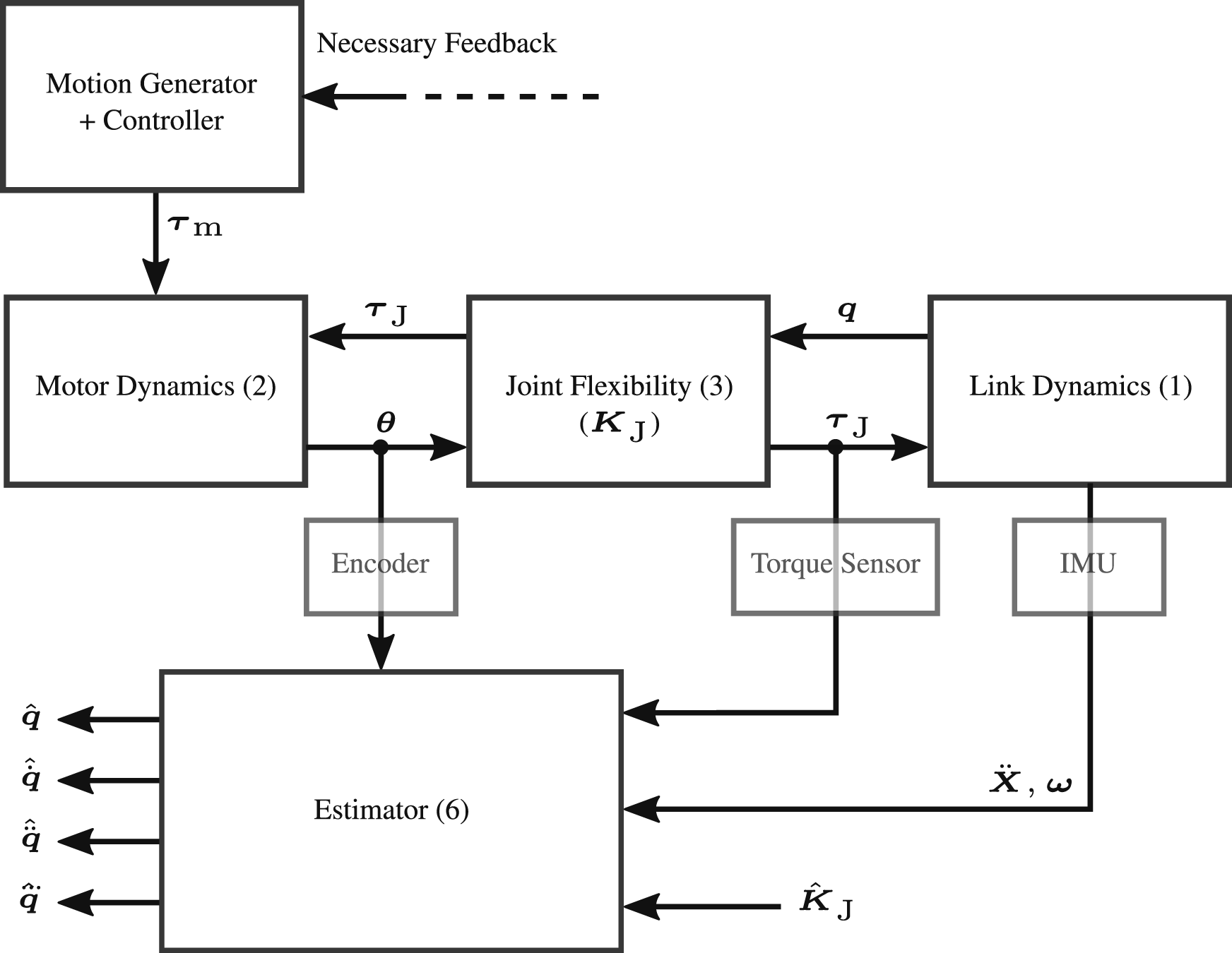
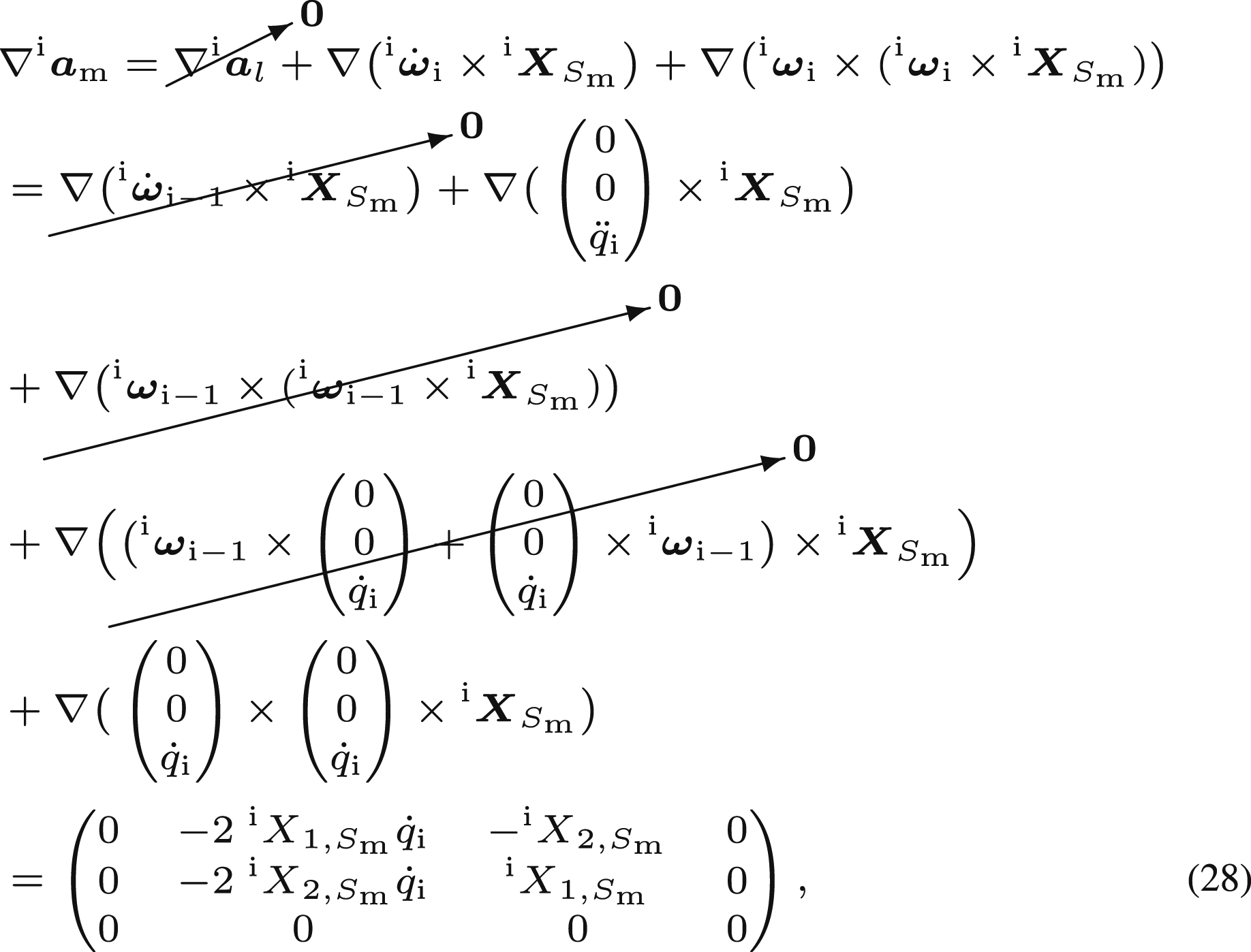
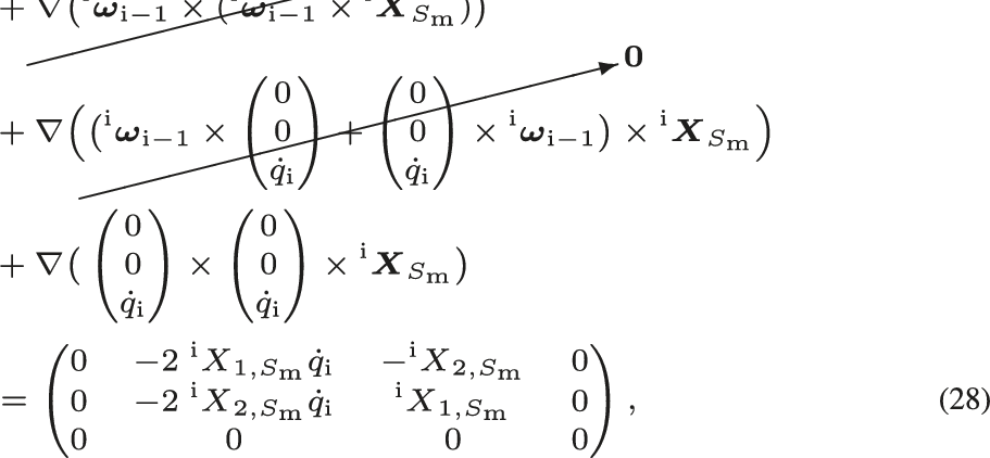
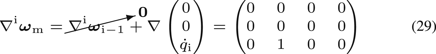
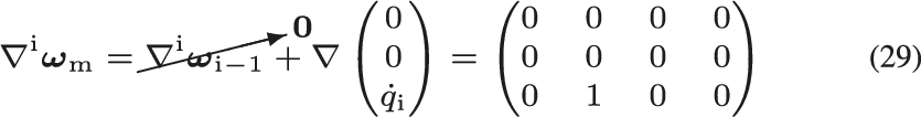
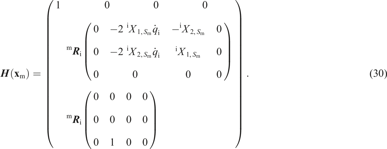
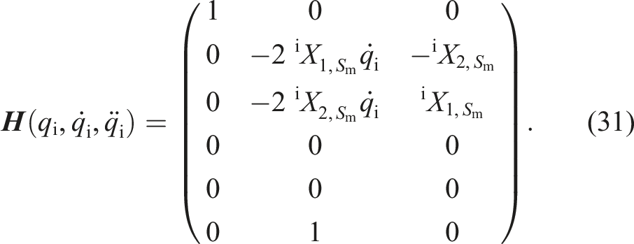
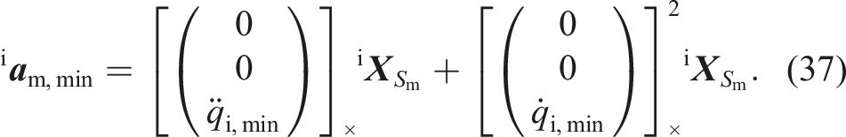
For the nonlinear estimator to operate properly, it is necessary to identify and fully formulate the measurement function in equation (6). This enables the filter to compute and compare the actual sensor measurements with their predicted counterparts and, consequently, to update the estimator gain. Therefore, in this section, we briefly characterize the components in the measurement function. The Cartesian link acceleration ${}^{\text{m}}\mathit{a}_{\text{m}}$ and angular velocity ${}^{\text{m}}\mathit{\omega }_{\text{m}}$ used in the measurement function are measured by the IMUs installed on the i-th link. Specifically, they can be modeled based on the estimator states via (Craig, 2006)

$\begin{array}{l}\hfill {}^{\mathrm{i}}\mathit{a}_{\text{m}}={}^{\mathrm{i}}\mathit{a}_l+{}^{\mathrm{i}}\dot{\mathit{\omega }}_{\text{i}}\times {}^{\mathrm{i}}\mathit{X}_{S_{\text{m}}}+{}^{\mathrm{i}}\mathit{\omega }_{\text{i}}\times \left({}^{\mathrm{i}}\mathit{\omega }_{\text{i}}\times {}^{\mathrm{i}}\mathit{X}_{S_{\text{m}}}\right),\end{array}$

(7)

$\begin{array}{l}\hfill \left(\begin{array}{c}\hfill 0\hfill \\ \hfill 0\hfill \\ \hfill {\dot{q}}_{\text{i}}\hfill \end{array}\right)={}^{\mathrm{i}}\mathit{\omega }_{\text{i}}-{}^{\mathrm{i}}\mathit{\omega }_{\text{i}-1},\left(\begin{array}{c}\hfill 0\hfill \\ \hfill 0\hfill \\ \hfill {\ddot{q}}_{\text{i}}\hfill \end{array}\right)={}^{\text{i}}\dot{\mathit{\omega }}_{\text{i}}-{}^{\mathrm{i}}\dot{\mathit{\omega }}_{\text{i}-1},\end{array}$

(8)

where ${}^{\mathrm{i}}\mathit{X}_{S_{\text{m}}}={[{}^{\text{i}}X_{1,S_{\text{m}}},{}^{\text{i}}X_{2,S_{\text{m}}},{}^{\text{i}}X_{3,S_{\text{m}}}]}^T\in {\mathbb{R}}^3$ and ${}^{\mathrm{i}}\mathit{a}_l\in {\mathbb{R}}^3$ denote the fixed location of sensor S_m w.r.t. joint frame {i} and the linear link acceleration, respectively. Furthermore, ${}^{\mathrm{i}}\mathit{a}_{\text{m}}$ and ${}^{\text{i}}\mathit{\omega }_{\text{i}}$ are the Cartesian acceleration and angular velocity at the location of sensor S_m expressed in joint frame {i}, respectively. Finally, ${}^{\mathrm{i}}\mathit{a}_{\text{m}}$ and ${}^{\text{i}}\mathit{\omega }_{\text{m}}={}^{\mathrm{i}}\mathit{\omega }_{\mathrm{i}}$ need to be rotated to the sensor frame {m} via the rotation matrix ${}^{\mathrm{m}}\mathit{R}_{\mathrm{i}}$ .

${}^{\mathrm{m}}\mathit{a}_{\text{m}}={}^{\mathrm{m}}\mathit{R}_{\mathrm{i}}{}^{\mathrm{i}}\mathit{a}_{\text{m}},{}^{\text{m}}\mathit{\omega }_{\text{m}}={}^{\mathrm{m}}\mathit{R}_{\mathrm{i}}{}^{\mathrm{i}}\mathit{\omega }_{\mathrm{m}}.$

(9)

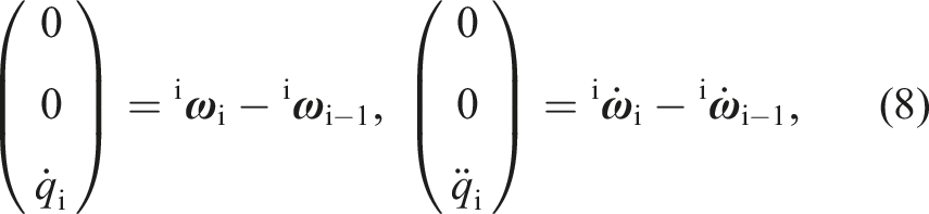
Note that since the angular velocity of a rigid body is independent of the measurement location, ${}^{\text{i}}\mathit{\omega }_{\text{m}}={}^{\mathrm{i}}\mathit{\omega }_{\mathrm{i}}$ holds. As can be observed from equations (7) and (8), the measurement function is built recursively starting from the stationary base (i = 0) to the last link (i = n). Note that we calibrate offline both the robot (Appendixe A.1) and the IMUs (Appendixe A.6) before running the system. Therefore, we may form a forward kinematics function for each IMU as

${}^0\mathit{T}_{\text{m}}={}^0\mathit{T}_{\text{i}}{}^{\text{i}}\mathit{T}_{\text{m}},$

(10)

where ${}^0\mathit{T}_{\text{IMU}}$ is the homogeneous transformation between IMU and base frame, containing both translation and orientation of the IMU w.r.t. the robot base. ${}^0\mathit{T}_{\text{i}}$ is the homogeneous transformation between the joint i and the robot base, obtained through robot calibration (Appendixe A.1). Finally, ${}^{\text{i}}\mathit{T}_{\text{IMU}}$ is the constant pose of the IMU w.r.t. the joint i frame, obtained through IMU calibration (Appendixe A.6). Therefore, the rotation matrix ${}^{\mathrm{m}}\mathit{R}_{\mathrm{i}}$ in equation (9) is available at any given time. If integrated IMU sensors become a commodity in robotics, ${}^{\mathrm{m}}\mathit{R}_{\mathrm{i}}$ can be provided by the manufacturer.

In an articulated manipulator with a stationary base, the linear acceleration 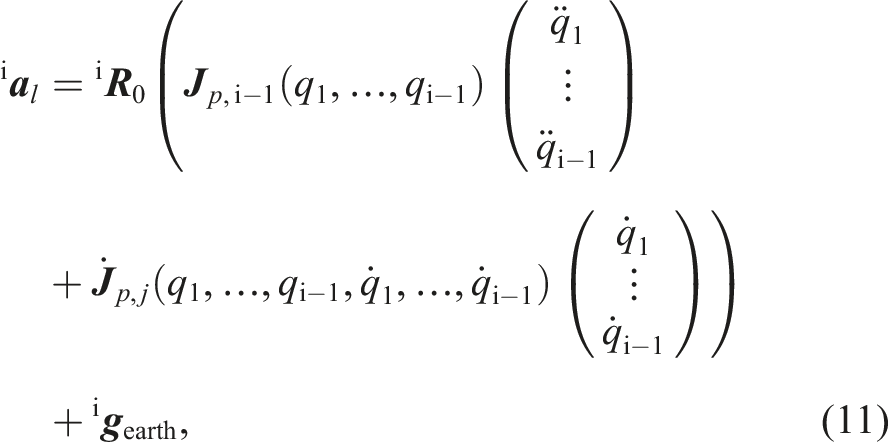${}^{\mathrm{i}}\mathit{a}_l$ in equation (7) is completely determined by upstream joint motions and gravity, that is,

$\begin{array}{ll}{}^{\mathrm{i}}\mathit{a}_l\hfill & ={}^{\mathrm{i}}\mathit{R}_0({\mathit{J}}_{p,\mathrm{i}-\mathrm{1}}(q_1,\dots ,q_{\text{i}-1})\left(\begin{array}{c}\hfill {\ddot{q}}_1\hfill \\ \hfill ⋮\hfill \\ \hfill {\ddot{q}}_{\text{i}-1}\hfill \end{array}\right)\hfill \\ \hfill & +{\dot{\mathit{J}}}_{p,j}(q_1,\dots ,q_{\text{i}-1},{\dot{q}}_1,\dots ,{\dot{q}}_{\text{i}-1})\left.\left(\begin{array}{c}\hfill {\dot{q}}_1\hfill \\ \hfill ⋮\hfill \\ \hfill {\dot{q}}_{\text{i}-1}\hfill \end{array}\right)\right)\hfill \\ \hfill & +{}^{\mathrm{i}}\mathit{g}_{\text{earth}},\hfill \end{array}$

(11)

where ${\mathit{J}}_{p,j}(\cdot ):{\mathbb{R}}^j\to {\mathbb{R}}^{3\times j}$ maps the joint motions up to joint $\mathit{j}$ to the Cartesian translational acceleration of the { $\text{i}$ }-frame origin. Moreover, ${\dot{\mathit{J}}}_{p,j}(\cdot ):{\mathbb{R}}^j\times {\mathbb{R}}^j\to {\mathbb{R}}^{3\times j}$ is the time derivative of J _p,j (⋅). As mentioned earlier, our method recursively communicates the kinematic states from the first link to the last link. Thus, the upstream states ${\dot{q}}_j$ and ${\ddot{q}}_j$ for j ∈ {1, 2, …, i − 1} are available at any given link i. Moreover, with the base at rest, the gravity contribution is handled by propagating the constant earth gravity vector ${}^0\mathit{g}_{\text{earth}}\in {\mathbb{R}}^3$ into the relevant frame:

${}^{\mathrm{i}}\mathit{g}_{\text{earth}}={}^{\text{i}}{{\mathit{R}}_0}^0{\mathit{g}}_{\text{earth}}.$

(12)

Note: Classical point estimation methods map the observations into parameter space, such that some goodness-of-fit criteria are met. When the relationship between random variables (measurements y _m in our case) and parameters (state vector x_m in our case) are described via an explicit mathematical model (similar to equation (6)), the estimation criteria fall into two categories, namely, maximum likelihood and maximum a posteriori estimation (Kulhavỳ, 1996). Generally speaking, the former optimizes for parameters such that the observations become most probable, therefore they maximize the conditional density function to maximize the corresponding likelihood function $\mathcal{L}({\mathbf{x}}_{\text{m}}|{\mathit{y}}_{\text{m}})=f({\mathit{y}}_{\text{m}}|{\mathbf{x}}_{\text{m}})$ . Here, f ( y _m| x _m) is the conditional density function of the observations given parameters. The latter, however, strives to find the most probable parameter based on the newly-added observation. In other words, they maximize the conditional density function of the parameter, given the latest observation f ( x _m| y _m). Therefore, these filter types are more suitable to be used in the recursive manner (Kamen and Su, 1999). Maximum a posteriori methods are intrinsically based on Bayes’ theorem. There exist several nonlinear Bayesian filtering methods, such as extended Kalman filter (EKF), unscented Kalman filter (UKF), strong tracking filter (STF), and particle filter (PF). EKF linearizes the system around the actual state via a Taylor approximation method. Therefore, EKF works well when the system nonlinearities are not severe (Feng et al., 2011). Since in system equation (6), the state transition function is linear and the measurement function nonlinearity is minor (second order polynomial), we use an EKF as nonlinear estimator for estimating the link-side variables in this article. Details on standard implementations can be found in Brown and Hwang (2012).

Nevertheless, we can use the estimated link variables to estimate the Cartesian position and velocity of an arbitrary point, which is rigidly attached to the robot manipulator. In the next section, we briefly review the forward kinematics approach for estimating Cartesian position and velocity.

Cartesian position and velocity estimation

Given an arbitrary position $\mathit{X}\in {\mathbb{R}}^6$ expressed in the robot base frame, it can be defined anywhere on the robot structure or an attached object to the end-effector, with the corresponding end-effector representation ${\mathit{X}}_{\text{ee}}\in {\mathrm{ℝ}}^6$ . Here, we assume that this position is rigidly connected to the robot end-effector. Therefore, the Cartesian velocity $\dot{\mathit{X}}\in {\mathbb{R}}^6$ of this position is given by

$\dot{\mathit{X}}={\mathit{J}}_{\text{p}}{\dot{\mathit{X}}}_{\text{ee}},$

(13)

where ${\dot{\mathit{X}}}_{\text{ee}}\in {\mathbb{R}}^6$ is the end-effector Cartesian velocity and ${\mathit{J}}_{\text{p}}\in {\mathbb{R}}^{6\times 6}$ is the Jacobian matrix defined by

${\mathit{J}}_{\text{p}}=\left[\begin{array}{cc}\hfill {\mathcal{I}}_3\hfill & \hfill {[{}^{\text{ee}}\mathit{p}]}_{\times }^T\hfill \\ \hfill {\mathit{0}}_{3\times 3}\hfill & \hfill {\mathcal{I}}_3\hfill \end{array}\right].$

(14)

Here, ${\mathcal{I}}_3\in {\mathbb{R}}^{3\times 3}$ is the identity matrix, ${}^{\text{ee}}\mathit{p}\in {\mathbb{R}}^3$ is the location of the position X in the end-effector frame {ee}, and [⋅]_× is the skew-symmetric matrix representation of a vector. Moreover, the manipulator Jacobian matrix ${\mathit{J}}_{\text{ee}}(q)\in {\mathbb{R}}^{6\times n}$ is given by

${\mathit{J}}_{\text{ee}}(q)=\frac{\partial {\mathit{X}}_{\text{ee}}(\mathit{q})}{\partial \mathit{q}}.$

(15)

Thus, we can map the link velocity $\dot{\mathit{q}}$ to Cartesian velocity $\dot{\mathit{X}}\in {\mathrm{ℝ}}^3$ of a given position X by substituting equation (15) into equation (13), giving

$\dot{\mathit{X}}={\mathit{J}}_{\text{p}}{\mathit{J}}_{\text{ee}}\left(\mathit{q}\right)\dot{\mathit{q}}=\mathit{J}\left(\mathit{q}\right)\dot{\mathit{q}}\mathbf{.}$

(16)

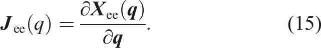
As shown in Baradaran Birjandi et al. (2022), the Cartesian velocity 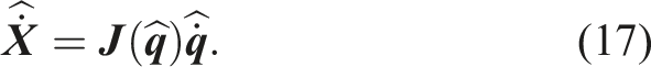$\widehat{\dot{\mathit{X}}}\in {\mathbb{R}}^6$ of a given position on the robot can be estimated via forward kinematics, as

$\widehat{\dot{\mathit{X}}}=\mathit{J}(\widehat{\mathit{q}})\widehat{\dot{\mathit{q}}}.$

(17)

Here, $\widehat{\mathit{q}}\in {\mathbb{R}}^n$ and $\widehat{\dot{\mathit{q}}}\in {\mathbb{R}}^n$ are the recursively estimated link angles and velocities using equation (6) for all links i = 1 to n.

Figure 4 summarizes different states and mathematical spaces that are discussed in Sections Link Velocity and Acceleration Estimation and Cartesian Position and Velocity Estimation. Now that the estimation procedure has been established, let us consider the IMU placement problem.

Figure 4.

Transformation of random variables into different spaces.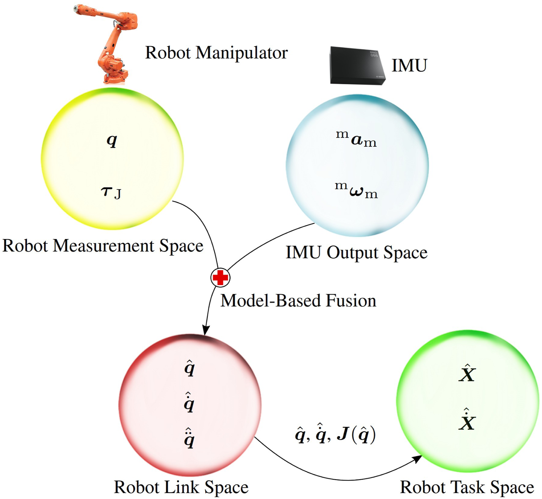

IMU sensor placement

In this section, we deal with three topics regarding sensor placement. We first address the question of how to optimally place the IMUs within the robot structure based on FIM theory. Herein, FIM provides insight into how much information a single sensor provides. Accordingly, we formulate an optimization problem where this information is maximized by manipulating the sensor position. Subsequently, the problem of a lower bound SNR is addressed. More specifically, we identify the worst sensor position, where the sensor signal is still recognizable from the background noise. As a result, a lower bound on the estimation accuracy is established. Finally, the sensor position is optimized such that collision detection via IMUs becomes applicable. In other words, we aim to place the sensor such that the vibrations of an unforeseen—both temporally and spatially—collision with the robot are detected by the sensor with minimum delay. The question of placing IMUs is especially relevant when designing a robot. This section provides an overview of the problem for mechatronics engineers.

Accelerometer signal-to-noise ratio

Before discussing the sensor placement problem, it is worth mentioning the accelerometer signal-to-noise ratio. This would highlight the importance of sensor placement. According to equation (11), the linear acceleration a _l is independent of the measurement point. However, the tangential and centripetal acceleration amplitude is directly related to the distance from the rotation axis. In fact, the greater the distance from the rotation axis $({}^{\mathrm{i}}\mathit{X}_{S_{\text{m}}})$ , the larger the angular acceleration amplitude and, consequently, the measured acceleration magnitude ${}^{\text{m}}\mathit{a}$ becomes. This is an important property that determines the accelerometer signal contribution to the estimator, especially in the presence of additive measurement noise. In other words, the signal is recognizable only if

$\text{SNR}=\frac{P_{\text{s}}}{P_{\text{n}}}$

(18)

is high enough ³ . Here, P_s and P_n are the signal and noise power, respectively. SNR is usually expressed in decibels. In order to increase the accelerometer SNR, we propose two methods in this section.

Method 1

In the first method, we aim to increase the signal power. The intuitive approach for this is to increase the sensor distance from the rotation axis $({}^{\mathrm{i}}\mathit{X}_{S_{\text{m}}})$ . Let us detail this in the FIM sense. FIM is a measure of the amount of information provided by an observation. It is defined as (Mutambara, 2019)

$\mathit{I}=-\mathbb{E}[\nabla {\nabla }^T\ln \mathcal{L}({\mathbf{x}}_{\text{m}}|{\mathit{y}}_{\text{m}})],$

(19)

where ∇ denotes the Nabla operator w.r.t. the state vector x_m and $\mathbb{E}[\cdot ]$ the expected value. For an unbiased estimator, simplifying equation (19) yields (Crassidis and Junkins, 2011)

$\begin{array}{ll}\hfill \mathit{I}& ={\mathit{H}}^T{\mathit{S}}^{-1}\mathit{H},\hfill \\ \text{with\hspace{0.17em}}\mathit{H}\hfill & =\nabla {\mathit{y}}_{\text{m}},\hfill \end{array}$

(20)

where H is the observation (or measurement) matrix and $\mathit{S}=\mathbb{E}[\mathit{v}{\mathit{v}}^T]$ is the measurement noise covariance matrix. Assuming Gaussian measurement noise, the information matrix can be shown to be the inverse of the estimation error covariance (Mutambara, 2019; Crassidis and Junkins, 2011)

$\mathbb{E}\left[\left({\mathbf{x}}_{\text{m}}-{\widehat{\mathbf{x}}}_{\text{m}}\right){\left({\mathbf{x}}_{\text{m}}-{\widehat{\mathbf{x}}}_{\text{m}}\right)}^T\right]={\mathit{I}}^{-1}.$

(21)

The covariance matrix characterizes the estimation confidence; that is, the smaller the estimation error $\left({\mathbf{x}}_{\text{m}}-{\widehat{\mathbf{x}}}_{\text{m}}\right)$ is, the more accurate the estimation will be. Equivalently, maximizing the determinant of the observation information matrix

$\underset{\mathit{H}}{\max }\text{det}\left(\mathit{I}\right)=\underset{\mathit{H}}{\max }\text{det}\left({\mathit{H}}^T{\mathit{S}}^{-1}\mathit{H}\right),$

(22)

increases the estimation confidence (Crassidis and Junkins, 2011) or decreases the geometric mean of the estimation error (Faller et al., 2003). For applying this sensor information optimization framework, the observation matrix H —which corresponds to the linearized measurement function y in equation (6)—needs to be obtained via

$\mathit{H}\left({\mathbf{x}}_{\text{m}}\right)=\nabla {\mathit{y}}_{\text{m}}\left({\mathbf{x}}_{\text{m}}\right)=\left(\begin{array}{c}\nabla q_{\text{i}}\\ {\nabla }^{\text{m}}{\mathit{a}}_{\text{m}}\left({\mathbf{x}}_{\text{m}}\right)\\ {\nabla }^{\text{m}}{\mathit{\omega }}_{\text{m}}\left({\mathbf{x}}_{\text{m}}\right)\end{array}\right).$

(23)

In order to derive H , take the following properties of cross product for three arbitrary vectors $\mathit{a},\mathit{b},\mathit{c}\in {\mathbb{R}}^3$ (Hogben, 2006):

$\begin{array}{ll}\hfill & \mathit{a}\times \mathit{b}=-\mathit{b}\times \mathit{a}\hfill \end{array}$

(24)

$\begin{array}{ll}\hfill & (\mathit{a}+\mathit{b})\times \mathit{c}=\mathit{a}\times \mathit{c}+\mathit{b}\times \mathit{c}\hfill \end{array}$

(25)

$\begin{array}{ll}\hfill & \frac{\text{d}}{\text{d}t}(\mathit{a}\times \mathit{b})=\frac{\text{d}\mathit{a}}{\text{d}t}\times \mathit{b}+\mathit{a}\times \frac{\text{d}\mathit{b}}{\text{d}t}\hfill \end{array}$

(26)

$\begin{array}{ll}\hfill & \mathit{a}\times \mathit{b}=\left(\begin{array}{ccc}\hfill 0\hfill & \hfill -a_3\hfill & \hfill a_2\hfill \\ \hfill a_3\hfill & \hfill 0\hfill & \hfill -a_1\hfill \\ \hfill -a_2\hfill & \hfill a_1\hfill & \hfill 0\hfill \end{array}\right)\mathit{b}={[\mathit{a}]}_{\times }\mathit{b},\hfill \end{array}$

(27)

where [ a ]_× is a skew-symmetric matrix. Thus, according to equation (8)

(28)

where 0 = [0 0 0] ^T . Note that we are optimizing the sensor $\text{position\hspace{0.17em}}{}^{\mathrm{i}}\mathit{X}_{S_{\text{m}}}$ w.r.t. the current link i and its motion. Accordingly, contributions from upstream link motions are neglected, assuming that their kinematic states are already accurately estimated by IMUs optimally placed on preceding links. Consequently, the current link i estimation accuracy must be adjusted by optimally placing the IMUs on the current link. Also,

(29)

is the Jacobian of the angular velocity measured at the sensor location and w.r.t. the link frame {i}. Substituting equations (28) and (29) into equation (23), one obtains

$\begin{array}{l}\hfill \mathit{H}({\mathbf{x}}_{\text{m}})=\left(\begin{array}{cccc}\hfill 1\hfill & \hfill 0\hfill & \hfill 0\hfill & \hfill 0\hfill \\ \hfill {}^{\mathrm{m}}\mathit{R}_{\mathrm{i}}\hfill & \hfill (\begin{array}{cccc}\hfill 0\hfill & \hfill -2{}^{\text{i}}X_{1,S_{\text{m}}}{\dot{q}}_{\text{i}}\hfill & \hfill -{}^{\text{i}}X_{2,S_{\text{m}}}\hfill & \hfill 0\hfill \\ \hfill 0\hfill & \hfill -2{}^{\text{i}}X_{2,S_{\text{m}}}{\dot{q}}_{\text{i}}\hfill & \hfill {}^{\text{i}}X_{1,S_{\text{m}}}\hfill & \hfill 0\hfill \\ \hfill 0\hfill & \hfill 0\hfill & \hfill 0\hfill & \hfill 0\hfill \end{array})\hfill \\ \hfill {}^{\mathrm{m}}\mathit{R}_{\mathrm{i}}\hfill & \hfill (\begin{array}{cccc}\hfill 0\hfill & \hfill 0\hfill & \hfill 0\hfill & \hfill 0\hfill \\ \hfill 0\hfill & \hfill 0\hfill & \hfill 0\hfill & \hfill 0\hfill \\ \hfill 0\hfill & \hfill 1\hfill & \hfill 0\hfill & \hfill 0\hfill \end{array})\hfill \end{array}\right).\end{array}$

(30)

As can be seen, H is independent of the link jerk ${\stackrel{\dots }{q}}_{\text{i}}$ . In other words, the fourth column contains only zeros, and is omitted for the sake of simplicity. Now, let IMU S_m be aligned with the link frame {i}, that is, ${}^{\mathrm{m}}\mathit{R}_{\mathrm{i}}={\mathcal{I}}_3$ , with ${\mathcal{I}}_3$ being the identity matrix of size 3. Therefore, H simplifies to

$\mathit{H}(q_{\text{i}},{\dot{q}}_{\text{i}},{\ddot{q}}_{\text{i}})=\left(\begin{array}{ccc}1& 0& 0\\ 0& -2{}^{\text{i}}{X}_{1,S_{\text{m}}}^{}{\dot{q}}_{\text{i}}& {-}^{\text{i}}{X}_{2,S_{\text{m}}}\\ 0& -2{}^{\text{i}}{X}_{2,S_{\text{m}}}^{}{\dot{q}}_{\text{i}}& {}^{\text{i}}{X}_{1,S_{\text{m}}}\\ 0& 0& 0\\ 0& 0& 0\\ 0& 1& 0\end{array}\right).$

(31)

Here, we assume that the noise power for each sensor is constant. Moreover, let the uncorrelated measurement noise covariance matrix be $\mathit{S}=\text{diag}\{{\sigma }_q^2,{\mathit{\sigma }}_{\mathit{a}}^2,{\mathit{\sigma }}_{\mathit{\omega }}^2\}$ , with ${\sigma }_q^2\in \mathbb{R}$ , ${\mathit{\sigma }}_{\mathit{a}}^2={[{\sigma }_{1,\mathit{a}}^2,{\sigma }_{2,\mathit{a}}^2,{\sigma }_{3,\mathit{a}}^2]}^T\in {\mathbb{R}}^3$ and ${\mathit{\sigma }}_{\mathit{\omega }}^2={[{\sigma }_{1,\mathit{\omega }}^2,{\sigma }_{2,\mathit{\omega }}^2,{\sigma }_{3,\mathit{\omega }}^2]}^T\in {\mathbb{R}}^3$ being the constant measurement noise variance of link position measurement (derived from motor encoder and joint torque sensor measurements according to equation (6)), accelerometer and gyroscope, respectively. Finally, the determinant of the information matrix becomes

$\begin{array}{ll}\hfill \text{det}(\mathit{I})& =\frac{{\sigma }_{3,\mathit{\omega }}^2{q}_{\text{i}}^2{\left(2({}^{\text{i}}X_{1,S_{\text{m}}}^2+{}^{\text{i}}X_{2,S_{\text{m}}}^2)\right)}^2}{{\sigma }_q^2{\sigma }_{1,\mathit{a}}^2{\sigma }_{2,\mathit{a}}^2{\sigma }_{3,\mathit{\omega }}^2}\hfill \\ \hfill & +\frac{{\sigma }_{1,\mathit{a}}^2{}^{\text{i}}X_{1,S_{\text{m}}}^2+{\sigma }_{2,\mathit{a}}^2{}^{\text{i}}X_{2,S_{\text{m}}}^2}{{\sigma }_q^2{\sigma }_{1,\mathit{a}}^2{\sigma }_{2,\mathit{a}}^2{\sigma }_{3,\mathit{\omega }}^2}.\hfill \end{array}$

(32)

Therefore, increasing the sensor distance from the rotation axis along the perpendicular axes ( ${}^{\text{i}}X_{1,S_{\text{m}}}$ or ${}^{\text{i}}X_{2,S_{\text{m}}}$ ), increases the amount of information provided by the IMU, and in particular the accelerometer. Note that according to equation (8), only acceleration is a function of the sensor location. Moreover, depending on the rotation axis, rotating the sensor might change the measurement function and, consequently, the observation matrix. However, regardless of its orientation ${}^{\mathrm{m}}\mathit{R}_{\text{i}}$ , increasing the sensor distance from the rotation axis will always increase the determinant of the corresponding information matrix. This is a direct result of the rotation matrix orthogonality; that is,

$\begin{array}{ll}{\Vert }^{\text{m}}{\mathit{a}}_{\text{m}}{\Vert }_2& ={\Vert {}^{\mathrm{m}}\mathit{R}_{\mathrm{i}}}^{\text{i}}{\mathit{a}}_{\text{m}}{\Vert }_2=\sqrt{{}^{\text{i}}{{\mathit{a}}_{\text{m}}^T}^{\text{m}}{\mathit{R}}_{\text{i}}^T{{}^{\text{m}}{\mathit{R}}_{\text{i}}}^{\text{i}}{\mathit{a}}_{\text{m}}}\\ & =\Vert {}^{\text{i}}{\mathit{a}}_{\text{m}}^{}{\Vert }_2,\end{array}$

(33)

where ‖ ⋅‖₂ denotes the Euclidean norm. Note that this method is constrained to the robot’s mechatronic limitations. In other words, the sensor cannot be placed arbitrarily on the link.

Observability Analysis

Note that the full measurement matrix 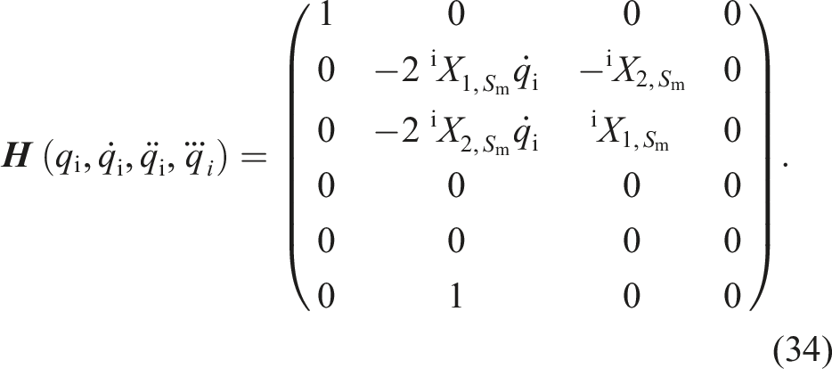$H(\cdot )\in {\mathbb{R}}^{7\times 4}$ (considering the link jerk) is given by

$\mathit{H}(q_{\text{i}},{\dot{q}}_{\text{i}},{\ddot{q}}_{\text{i}},{\stackrel{\dots }{q}}_i)=\left(\begin{array}{cccc}1& 0& 0& 0\\ 0& -2{}^{\text{i}}{X}_{1,S_{\text{m}}}^{}{\dot{q}}_{\text{i}}& -{}^{\text{i}}{X}_{2,S_{\text{m}}}& 0\\ 0& -2{}^{\text{i}}{X}_{2,S_{\text{m}}}^{}{\dot{q}}_{\text{i}}& {{}^{\text{i}}{X}_{1,S_{\text{m}}}}^{}& 0\\ 0& 0& 0& 0\\ 0& 0& 0& 0\\ 0& 1& 0& 0\end{array}\right).$

(34)

Accordingly, it can be shown that the observability matrix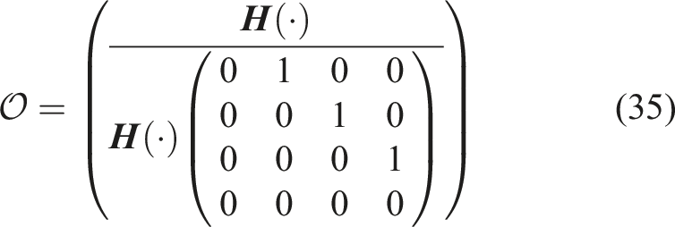

$\mathcal{O}=\left(\frac{\mathit{H}(\cdot )}{\mathit{H}(\cdot )\left(\begin{array}{cccc}\hfill 0\hfill & \hfill 1\hfill & \hfill 0\hfill & \hfill 0\hfill \\ \hfill 0\hfill & \hfill 0\hfill & \hfill 1\hfill & \hfill 0\hfill \\ \hfill 0\hfill & \hfill 0\hfill & \hfill 0\hfill & \hfill 1\hfill \\ \hfill 0\hfill & \hfill 0\hfill & \hfill 0\hfill & \hfill 0\hfill \end{array}\right)}\right)$

(35)

is of full rank (rank $(\mathcal{O})$ = 4) and thus, the system is locally observable.

Method 2

Another technique to overcome the low SNR is to reduce the noise power. This can be done by fusing multiple sensors. Multi-sensor data fusion is a technique to combine information from multiple sources (sensors here) to achieve inferences that cannot be obtained from a single sensor or whose quality exceeds that of an inference drawn from any single sensor (Liggins II et al., 2017). We have exemplified this in Appendix A.4. In the following sections, we mainly focus on the first method, where the accelerometer location is optimized.

Minimum estimation accuracy bound

From a design perspective, finding a meaningful lower bound for the accelerometer distance from the rotation axis is crucial. It depends on several factors, such as sensor resolution, noise power, and desired motion bandwidth. However, one first needs to determine the minimum link motion ranges to be detected by the accelerometer. For obtaining the minimum detectable sensor measurements, let us rewrite equation (8) as follows: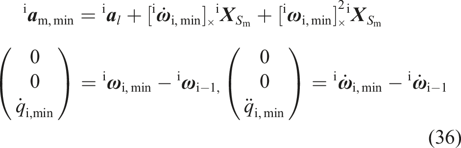

$\begin{array}{ll}\hfill {}^{\text{i}}\mathit{a}_{\mathrm{m},\mathrm{m}\mathrm{i}\mathrm{n}}& ={}^{\text{i}}\mathit{a}_l+{[{}^{\mathrm{i}}\dot{\mathit{\omega }}_{\mathrm{i},\text{min}}]}_{\times }{}^{\mathrm{i}}\mathit{X}_{S_{\text{m}}}+{[{}^{\mathrm{i}}\mathit{\omega }_{\mathrm{i},\text{min}}]}_{\times }^2{}^{\mathrm{i}}\mathit{X}_{S_{\text{m}}}\hfill \\ \hfill \left(\begin{array}{c}\hfill 0\hfill \\ \hfill 0\hfill \\ \hfill {\dot{q}}_{\text{i,min}}\hfill \end{array}\right)& ={}^{\mathrm{i}}\mathit{\omega }_{\mathrm{i},\text{min}}-{}^{\mathrm{i}}\mathit{\omega }_{\mathrm{i}-\mathrm{1},}\left(\begin{array}{c}\hfill 0\hfill \\ \hfill 0\hfill \\ \hfill {\ddot{q}}_{\mathrm{i},\text{min}}\hfill \end{array}\right)={}^{\mathrm{i}}\dot{\mathit{\omega }}_{\mathrm{i},\text{min}}-{}^{\mathrm{i}}\dot{\mathit{\omega }}_{\mathrm{i}-\mathrm{1}}\hfill \end{array}$

(36)

Then, ${}^{\mathrm{i}}\mathit{a}_{\mathrm{m},\text{min}}$ is rotated to ${}^{\mathrm{m}}\mathit{a}_{\mathrm{m},\text{min}}$ by equation (9). The minimum Cartesian acceleration ${}^{\mathrm{m}}\mathit{a}_{\mathrm{m},\text{min}}$ of link i, measured by sensor S_m needs to reflect the minimum velocity and acceleration of link i only. Here, contributions from upstream links must be eliminated from equation (36). Accordingly, all motions from previous links, that is, ${\dot{q}}_1=\cdots ={\dot{q}}_{\text{i}-1}=0$ and ${\ddot{q}}_1=\cdots ={\ddot{q}}_{\text{i}-1}=0$ are set to zero, and gravity effects are neglected for the purpose of deriving the minimum detectable acceleration. Therefore, ${}^{\mathrm{i}}\mathit{a}_l=0$ holds. This simplifies equation (36) to

${}^{\mathrm{i}}\mathit{a}_{\mathrm{m},\text{min}}={\left[\left(\begin{array}{c}\hfill 0\hfill \\ \hfill 0\hfill \\ \hfill {\ddot{q}}_{\text{i},\text{min}}\hfill \end{array}\right)\right]}_{\times }{}^{\mathrm{i}}\mathit{X}_{S_{\text{m}}}+{\left[\left(\begin{array}{c}\hfill 0\hfill \\ \hfill 0\hfill \\ \hfill {\dot{q}}_{\text{i},\text{min}}\hfill \end{array}\right)\right]}_{\times }^2{}^{\mathrm{i}}\mathit{X}_{S_{\text{m}}}.$

(37)

At the same time, ${}^{\mathrm{m}}\mathit{a}_{\mathrm{m},\text{min}}$ is also determined by the available sensor sensitivity. It limits the smallest physical quantity that can be detected by the sensor to be

${}^{\mathrm{m}}\mathit{a}_{\mathrm{m},\text{min}}=\frac{\text{FS}}{2^{nb}},$

(38)

with FS being the sensor range or full scale and nb the number of sensor (quantization) bits. In a noise-free scenario, given the sensor sensitivity and also the minimum desired detectable link variables, equation (37) can be solved for ${}^{\mathrm{i}}\mathit{X}_{S_{\text{m}}}$ .

However, under realistic conditions with additive noise, the signal has to be distinguishable from noise. This may be formulated as a classical signal detection problem: A threshold above the estimated average noise power defines a simple boundary between the signals and noise. Smaller thresholds increase the probability of false detections due to noise. However, with larger thresholds, the signal power must also be higher to be detected (Swanson, 2000). As a result, this threshold is a compromise between false detection and minimum signal power.

In order to elaborate on this matter, we consider two different well-established criteria, namely, signal envelope detection and reduction of false alarm probability.

Signal envelope detection

Signal envelope detection is a concept mainly used in telecommunication systems, where the received signals need to be demodulated to the original ones, based on their envelope (Tretter, 2008). The problem is relevant here, as the original signal power—and consequently its SNR—plays an important role in the demodulated signal quality, when it is corrupted by noise in the channel. Equivalently, in our problem, one needs to improve the measured signal quality relative to background noise (SNR) by appropriately choosing the sensor location, such that the signal can be detected by the sensor. In order to find the suitable sensor location where the signal envelope is detectable, the following steps are taken:

1. Based on the application requirements, the minimum desired SNR ⁴ is deduced. Here, SNR is a representative measure for a minimum detectable signal.

2. Subsequently, based on the chosen SNR, the minimum signal power as well as the minimum signal amplitude can be obtained.

3. With the calculated minimum signal amplitude, the sensor location is computed with equation (37). Naturally, the mechanical design options constitute further constraints.

By rearranging equation (18), we have

$P_s=\text{SNR}{P}_n=A_{\text{rms}}^2,$

(39)

where A_rms denotes the signal root mean square (RMS) amplitude (Gaydecki, 2004)

$A_{\text{rms}}=\sqrt{\frac{1}{T}{\int }_{t=0}^T{}^{\text{m}}\mathit{a}_{\text{m}}^2(t)\text{d}t}.$

(40)

Here, ${}^{\text{m}}\mathit{a}_{\text{m}}(t)$ with t ∈ [0 T] is a system and/or task-specific Cartesian acceleration trajectory. For sensor location design purposes, a quasi-instantaneous (worst-case) evaluation (T → 0) can be assumed. In other words, with the chosen minimum SNR, the sensor signal has to be distinguishable from the background noise at any given time. Furthermore, since the IMU sampling frequency is considered to be much higher than the fastest robot dynamics, ${}^{\mathrm{m}}\mathit{a}_{\mathrm{m}}(t)={}^{\mathrm{m}}\mathit{a}_{\mathrm{m}}$ is assumed to be constant over the interval T, and therefore, $A_{\text{rms}}=\frac{1}{\sqrt{3}}{\Vert }^{\mathrm{m}}{\mathit{a}}_{\mathrm{m}}{\Vert }_2$ . Substituting minimum desired values into equation (39) and subsequently equation (40), one obtains ${}^{\mathrm{m}}\mathit{a}_{\mathrm{m},\mathrm{m}\mathrm{i}\mathrm{n}}$ . Finally, one can again use ${}^{\mathrm{m}}\mathit{a}_{\mathrm{m},\mathrm{m}\mathrm{i}\mathrm{n}}$ to solve equation (37) for ${}^{\mathrm{i}}\mathit{X}_{S_{\text{m}}}$ . We further elaborate on this problem in Appendixe A.2, where the theory is exemplified via a numerical one-link robot. SNR is formulated as the sensor distance from the rotation axis in this example. In Appendixe A.2, it is shown that the SNR improves when the accelerometer is placed farther from the link rotation axis.

False alarm probability

From the sensor placement perspective, another reasonable goal is to find a lower-bound for the sensor distance to the rotation axis such that a maximum tolerable false alarm rate is met. For the sake of conservativeness, a zero-amplitude signal A_rms = 0 is assumed and we seek to find an amplitude threshold above the respective noise level with noise amplitude A _n . More specifically, we seek a threshold A _T such that, given the noise probability density function p (A _n | A_rms = 0), the false alarm probability p_fa remains below a specified maximum allowable value p_fa,max (Swanson, 2000), as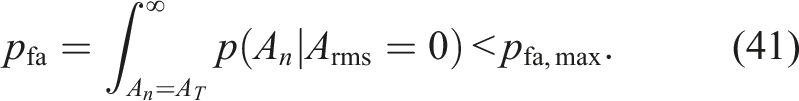

$p_{\text{fa}}={\int }_{A_n=A_T}^{\infty }p\left(A_n\right|A_{\text{rms}}=0)<p_{\text{fa},\text{max}}.$

(41)

Using equation (41), $A_T=\frac{1}{\sqrt{3}}{\Vert }^{\mathrm{m}}{\mathit{a}}_{\mathrm{m},\mathrm{m}\mathrm{i}\mathrm{n}}{\Vert }_2$ can be obtained and consequently, the minimum sensor distance from the rotation axis can be found via equation (37).

Finally, now that the essential design constraints signal envelope detection and false alarm probability can be expressed, we elaborate on this in the specific examples detailed in Appendixe A.2 (Example 2).

Multi-sensor fusion

Now, we address the problem of fusing multiple IMUs per link together with proprioceptive sensing for estimating link velocity and acceleration. As already described above, we have the choice between centralized and decentralized approaches. Both system architectures are introduced and analyzed next.

Centralized fusion

For linear systems with uncorrelated, zero-mean, white process and measurement noise, the Kalman filter is well known to be the optimal estimator in the least squares sense (Simon, 2006). Therefore, a centralized Kalman estimator is the optimal solution for linear multi-sensor systems. Since the nonlinearities in measurement function in equation (6) are not severe, a centralized EKF can be considered a viable sub-optimal solution for our system as well. Therefore, we establish a centralized scheme based on EKF estimator in this section. For both the linear and nonlinear cases, all system states are estimated within a single central estimator. As a result the augmented state transition function for our system becomes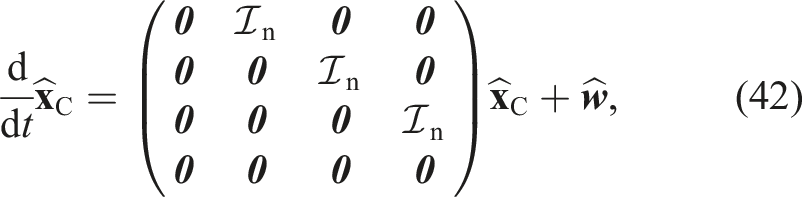

$\frac{\text{d}}{\text{d}t}{\widehat{\mathbf{x}}}_{\text{C}}=\left(\begin{array}{cccc}\hfill \mathit{0}\hfill & \hfill {\mathcal{I}}_{\text{n}}\hfill & \hfill \mathit{0}\hfill & \hfill \mathit{0}\hfill \\ \hfill \mathit{0}\hfill & \hfill \mathit{0}\hfill & \hfill {\mathcal{I}}_{\text{n}}\hfill & \hfill \mathit{0}\hfill \\ \hfill \mathit{0}\hfill & \hfill \mathit{0}\hfill & \hfill \mathit{0}\hfill & \hfill {\mathcal{I}}_{\text{n}}\hfill \\ \hfill \mathit{0}\hfill & \hfill \mathit{0}\hfill & \hfill \mathit{0}\hfill & \hfill \mathit{0}\hfill \end{array}\right){\widehat{\mathbf{x}}}_{\text{C}}+\widehat{\mathit{w}},$

(42)

where ${\widehat{\mathbf{x}}}_{\text{C}}={[{\widehat{\mathit{q}}}^T{\widehat{\dot{\mathit{q}}}}^T{\widehat{\ddot{\mathit{q}}}}^T{\widehat{\stackrel{⃛}{\mathit{q}}}}^T]}^T\in {\mathbb{R}}^{4\mathrm{n}}$ denotes the states along all $\mathrm{n}$ links and ${\mathcal{I}}_{\text{n}}$ is the identity matrix of size $\mathrm{n}$ . The augmented measurement function is given by

${\widehat{\mathit{y}}}_{\text{tot}}={\left(\begin{array}{cccccc}{\widehat{\mathit{y}}}_1^T& {\widehat{\mathit{y}}}_2^T& \cdots & {\widehat{\mathit{y}}}_{\text{m}}^T& \cdots & {\widehat{\mathit{y}}}_{\text{nl}}^T\end{array}\right)}^T+\widehat{\mathit{v}}.$

(43)

It is assumed that l IMUs are installed on each robot link. Thus, in total n × l IMUs are installed, and therefore, m ∈ {1, …, n × l}. Moreover, if IMUs m and m + 1 are installed on the same link, the corresponding y _m and y _m+1 share the same joint torque and motor position measurements, respectively. Figure 5 summarizes the centralized fusion for the considered system class, defined by equations (42) and (43), with $\text{n}$ links.

Figure 5.

Centralized elastic joint velocity and acceleration estimation.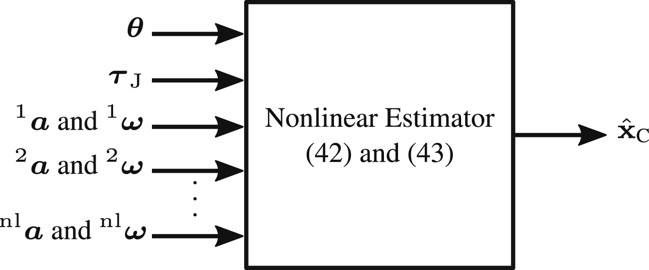

Decentralized fusion

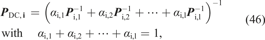
In the decentralized fusion architecture, the states are estimated in local estimators and fused via weighting coefficients. For linear systems the optimal weights can generally be computed under certain assumptions (Sun and Deng, 2004). However, this requires the estimation cross-covariance between every pair of local estimators to be known. For nonlinear systems such as the one described by equation (6), however, computing the cross covariance matrix at each epoch can be computationally very expensive. Therefore, in this work we adopt a sub-optimal method, widely known as covariance intersection (CI) algorithm, where the cross-covariance matrices are assumed to be unknown in decentralized fusion.

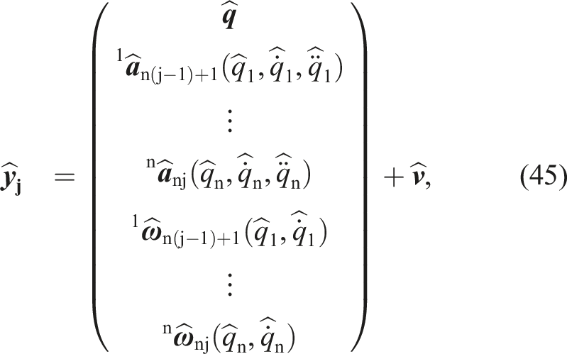
First, let us assume that each link has l IMUs. Therefore, there will be l local estimators in the considered setup. In each local estimator j, there exists the minimum number of required sensors (i.e., n IMUs) for estimating the link variables from link 1 to n. Local estimators share motor encoder and torque readings, but not IMUs. Thus, the IMUs in the j-th local estimator are counted via m ∈ {n (j − 1) + 1, n (j − 1) + 2, …, nj} from the first to the last link. Moreover, the j-th local estimator has the following dynamics model: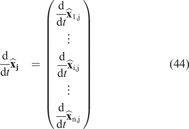

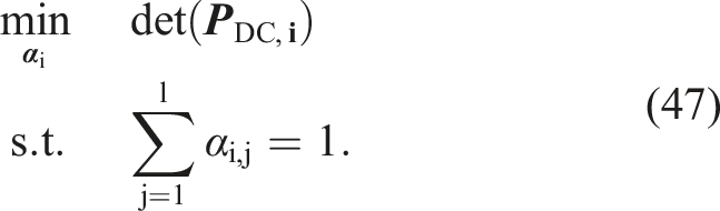
$\begin{array}{ll}\hfill \frac{\text{d}}{\text{d}t}{\widehat{\mathbf{x}}}_{\mathbf{j}}& =\left(\begin{array}{c}\hfill \frac{\text{d}}{\text{d}t}{\widehat{\mathbf{x}}}_{1\text{,j}}\hfill \\ \hfill ⋮\hfill \\ \hfill \frac{\text{d}}{\text{d}t}{\widehat{\mathbf{x}}}_{\text{i,j}}\hfill \\ \hfill ⋮\hfill \\ \hfill \frac{\text{d}}{\text{d}t}{\widehat{\mathbf{x}}}_{\text{n,j}}\hfill \end{array}\right)\hfill \end{array}$

(44)

$\begin{array}{ll}\hfill {\widehat{\mathit{y}}}_{\mathbf{j}}& =\left(\begin{array}{c}\hfill \widehat{\mathit{q}}\hfill \\ \hfill {}^1\widehat{\mathit{a}}_{\text{n}(\text{j}-1)+1}({\widehat{q}}_1,{\widehat{\dot{q}}}_1,{\widehat{\ddot{q}}}_1)\hfill \\ \hfill ⋮\hfill \\ \hfill {}^{\text{n}}\widehat{\mathit{a}}_{\text{nj}}({\widehat{q}}_{\text{n}},{\widehat{\dot{q}}}_{\text{n}},{\widehat{\ddot{q}}}_{\text{n}})\hfill \\ \hfill {}^1\widehat{\mathit{\omega }}_{\text{n}(\text{j}-1)+1}({\widehat{q}}_1,{\widehat{\dot{q}}}_1)\hfill \\ \hfill ⋮\hfill \\ \hfill {}^{\text{n}}\widehat{\mathit{\omega }}_{\text{nj}}({\widehat{q}}_{\text{n}},{\widehat{\dot{q}}}_{\text{n}})\hfill \end{array}\right)+\widehat{\mathit{v}},\hfill \end{array}$

(45)

where states are ${\widehat{\mathbf{x}}}_{\mathbf{j}}={[{\widehat{\mathbf{x}}}_{1\text{,j}}^T,\dots ,{\widehat{\mathbf{x}}}_{\text{i,j}}^T,\dots ,{\widehat{\mathbf{x}}}_{\text{n,j}}^T]}^T\in {\mathbb{R}}^{4\mathrm{n}}$ , with ${\widehat{\mathbf{x}}}_{\text{i,j}}={\left[{\widehat{q}}_{\text{i}},{\widehat{\dot{q}}}_{\text{i}},{\widehat{\ddot{q}}}_{\text{i}},{\widehat{\stackrel{⃛}{q}}}_{\text{i}}\right]}_{\text{j}}^T\in {\mathbb{R}}^4$ , from the first (i = 1) to the last link (i = n). The dynamics of each ${\widehat{\mathbf{x}}}_{\text{i,j}}$ are given by equation (6). Note that the states and measurements indices of the dynamics model (equation (45)) is denoted by the bold symbol j (as opposed to j), indicating that they represent stacked vectors of other states and measurements. Using the covariance-intersection algorithm the fused estimation error covariance of the i-th link is computed as (Julier and Uhlmann, 2017)

$\begin{array}{ll}\hfill {\mathit{P}}_{\text{DC},\mathbf{i}}& ={\left({\alpha }_{\text{i,}1}{\mathit{P}}_{\text{i,}1}^{-1}+{\alpha }_{\text{i,}2}{\mathit{P}}_{\text{i,}2}^{-1}+\cdots +{\alpha }_{\text{i,l}}{\mathit{P}}_{\text{i,l}}^{-1}\right)}^{-1}\hfill \\ \hfill \text{with\hspace{0.17em}}& {\alpha }_{\text{i,}1}+{\alpha }_{\text{i,}2}+\cdots +{\alpha }_{\text{i,l}}=1,\hfill \end{array}$

(46)

where ${\mathit{P}}_{\text{i,j}}\in {\mathbb{R}}^{4\times 4}$ is the j-th (j ∈ {1, …, l}) local estimation error covariance of the i-th link with the weight coefficient ${\alpha }_{\text{i,j}}\in {\mathbb{R}}^{+}$ . Different choices of the weight vector ${\mathit{\alpha }}_{\mathbf{i}}={[{\alpha }_{\text{i,}1},\dots ,{\alpha }_{\text{i,j}},\dots ,{\alpha }_{\text{i,l}}]}^T\in {\mathbb{R}}^{\text{l}}$ might be used to optimize different performance criteria, such as minimizing the trace or the determinant of P _{DC, i} ,

$\begin{array}{ll}\hfill \underset{{\mathit{\alpha }}_{\text{i}}}{\min }& \text{det}({\mathit{P}}_{\text{DC},\mathbf{i}})\hfill \\ \hfill \text{s.t.\hspace{0.17em}}& \sum _{\text{j}=1}^{\text{l}}{\alpha }_{\text{i,j}}=1.\hfill \end{array}$

(47)

Due to the positive semi-definiteness of covariance matrices, this can be shown that this problem is convex (Liggins II et al., 2017). Therefore, various optimization strategies can be applied to effectively solve it, spanning from classical methods such as Newton-Raphson to advanced techniques such as semi-definite and convex programming. These approaches are capable of minimizing a wide range of mathematical norms, making them versatile tools for finding the optimal weights in equation (47) (Liggins II et al., 2017). In practice and for the system described by equation (45), we propose to compute the fusion gains as follows. The objective of these gains is to optimally combine the local estimators. The following steps are recommended to be taken to obtain the gains:

1. The system moves along a trajectory and the estimated states of all local estimators are recorded. This trajectory should preferably be an excitation trajectory, which persistently excites all the system modes.

2. The exact estimation error covariance ${\mathit{P}}_{\text{i,j}}=\mathbb{E}\left[\left({\mathbf{x}}_{\text{i}}-{\widehat{\mathbf{x}}}_{\text{i,j}}\right){\left({\mathbf{x}}_{\text{i}}-{\widehat{\mathbf{x}}}_{\text{i,j}}\right)}^T\right]$ , with ground truth ${\mathbf{x}}_{\text{i}}={\left[q_{\text{i}},{\dot{q}}_{\text{i}},{\ddot{q}}_{\text{i}},{\stackrel{⃛}{q}}_{\text{i}}\right]}^T$ , for all local estimators is computed. Here, the exact position trajectory q_i is initially computed according to equation (3) and based on the encoder ${\mathrm{\theta }}_{\text{i}}$ and elastic-joint torque τ_J,i measurements (the stiffness matrix estimation ${\widehat{K}}_{\text{J,i}}$ is also available). In order to construct the ground truth states ${\mathbf{x}}_{\text{i}}$ , ${\dot{q}}_{\text{i}}$ , ${\ddot{q}}_{\text{i}}$ , ${\stackrel{⃛}{q}}_{\text{i}}$ are obtained via high-precision external tracking systems.

3. Solve equation (47) for computing the weights offline.

Once the weights are computed and based on the covariance intersection algorithm (Julier and Uhlmann, 2017), the multi-sensor fused state for the i-th link is given by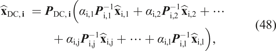

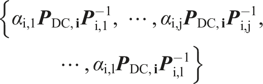
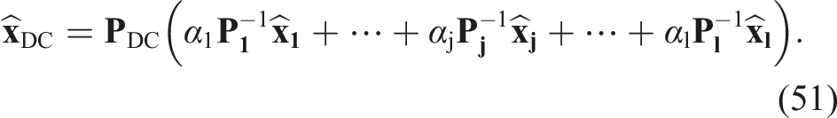
$\begin{array}{ll}\hfill {\widehat{\mathbf{x}}}_{\text{DC},\mathbf{i}}& ={\mathit{P}}_{\text{DC},\mathbf{i}}\left({\alpha }_{\text{i,}1}{\mathit{P}}_{\text{i,}1}^{-1}{\widehat{\mathbf{x}}}_{\text{i,}1}+{\alpha }_{\text{i,}2}{\mathit{P}}_{\text{i,}2}^{-1}{\widehat{\mathbf{x}}}_{\text{i,}2}+\cdots \right.\hfill \\ \hfill & +\left.{\alpha }_{\text{i,j}}{\mathit{P}}_{\text{i,j}}^{-1}{\widehat{\mathbf{x}}}_{\text{i,j}}+\cdots +{\alpha }_{\text{i,l}}{\mathit{P}}_{\text{i,l}}^{-1}{\widehat{\mathbf{x}}}_{\text{i,l}}\right),\hfill \end{array}$

(48)

where P _{DC, i} is formulated in equation (46). For the unrealistic assumption of absent cross-covariance between the estimated states $\{{\widehat{\mathbf{x}}}_{\text{i,}1},{\widehat{\mathbf{x}}}_{\text{i,}2},\dots ,{\widehat{\mathbf{x}}}_{\text{i,l}}\}$ , it is evident that the gains

$\begin{array}{l}\hfill \left\{{\alpha }_{\text{i,}1}{\mathit{P}}_{\text{DC},\mathbf{i}}{\mathit{P}}_{\text{i,}1}^{-1},\cdots ,{\alpha }_{\text{i,j}}{\mathit{P}}_{\text{DC},\mathbf{i}}{\mathit{P}}_{\text{i,j}}^{-1},\right.\\ \hfill \left.\cdots ,{\alpha }_{\text{i,l}}{\mathit{P}}_{\text{DC},\mathbf{i}}{\mathit{P}}_{\text{i,l}}^{-1}\right\}\end{array}$

are the optimal solutions in terms of squared error, which corresponds, for example, to minimizing the trace of equation (46). Moreover, the error covariance of the fused state ${\widehat{\mathbf{x}}}_{\text{DC},\mathbf{i}}$ remains bounded, as long as each individual error covariance P _i,j is bounded. In this case, we call the fused state ${\widehat{\mathbf{x}}}_{\text{DC},\mathbf{i}}$ consistent (Noack et al., 2017).

For the overall decentralized estimation 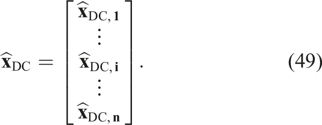${\widehat{\mathbf{x}}}_{\text{DC}}\in {\mathbb{R}}^{4\mathrm{n}}$ (encompassing all links), the fusion law is simply given by

${\widehat{\mathbf{x}}}_{\text{DC}}=\left[\begin{array}{c}\hfill {\widehat{\mathbf{x}}}_{\text{DC},\mathbf{1}}\hfill \\ \hfill ⋮\hfill \\ \hfill {\widehat{\mathbf{x}}}_{\text{DC},\mathbf{i}}\hfill \\ \hfill ⋮\hfill \\ \hfill {\widehat{\mathbf{x}}}_{\text{DC},\mathbf{n}}\hfill \end{array}\right].$

(49)

Figure 6 depicts the decentralized multi-sensor configuration together with the fault detection units that are detailed in the next section. In this figure, $\mathit{\alpha }=[{\mathit{\alpha }}_{\mathbf{1}},\dots ,{\mathit{\alpha }}_{\mathbf{i}},\dots ,{\mathit{\alpha }}_{\mathbf{n}}]\in {\mathbb{R}}^{\text{l}\times \mathrm{n}}$ .

Figure 6.

Decentralized multi-sensor fusion with FDI units.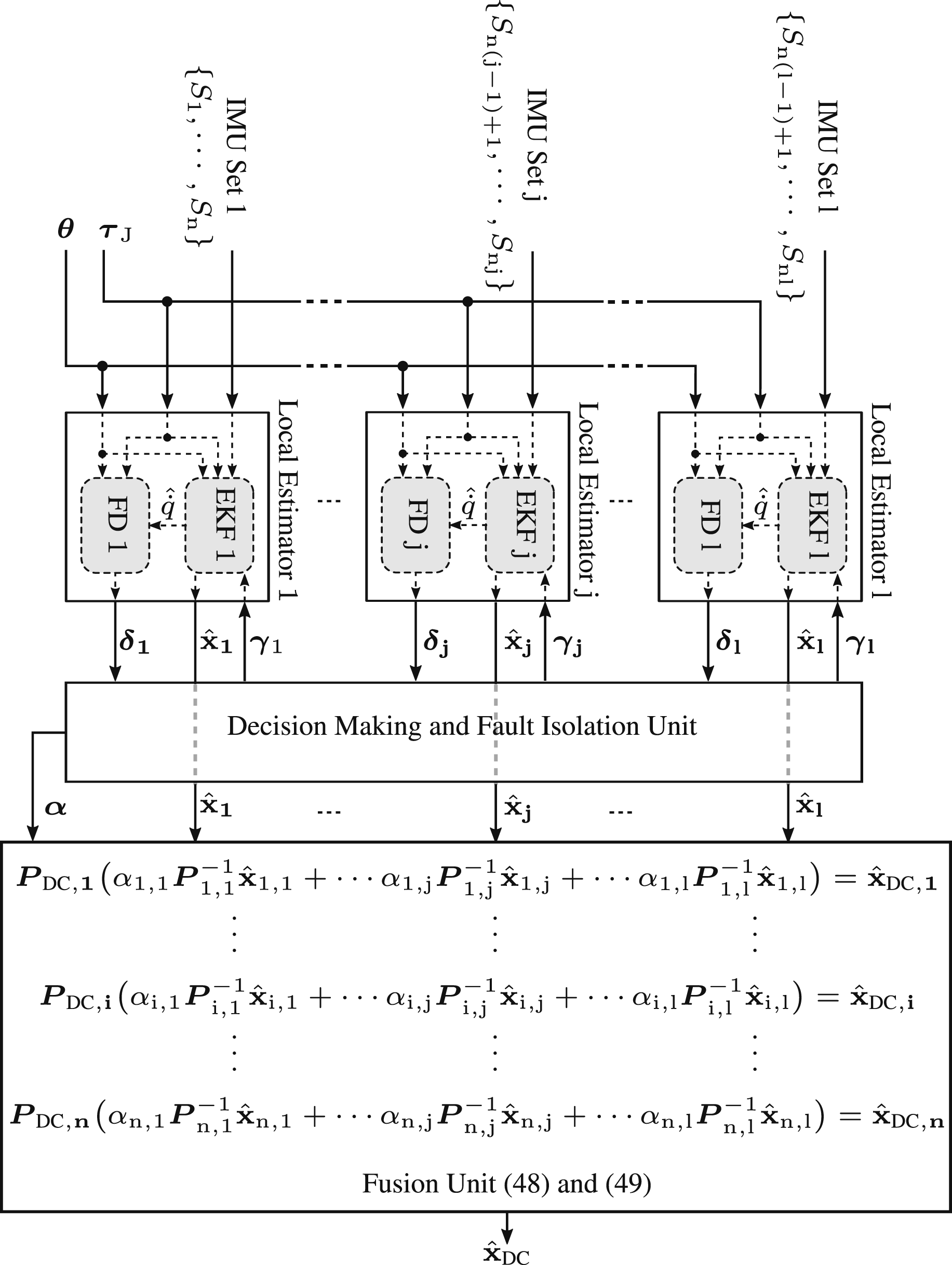

Furthermore, FD j and ${\mathit{\delta }}_{\mathbf{j}}=\{{\delta }_{1\text{,j}},\dots ,{\delta }_{\text{n,j}}\}\in {\mathbb{B}}^{\text{n}}$ , with $\mathbb{B}$ being the Boolean set, refer to the fault detection unit and the fault flag of the j-th local estimator, respectively. Moreover, ${\mathit{\gamma }}_{\mathbf{j}}=\{{\gamma }_{1\text{,j}},\dots ,{\gamma }_{\text{n,j}}\}\in {\mathbb{B}}^{\text{n}}$ denotes the isolation command.

This topology also allows fusing IMUs in non-symmetric setups. By symmetry we mean an equal number of IMUs per link. Consider, for example, that one link is equipped with three IMUs, while the successor has only one IMU. Therefore, α _i and α _i+1 will have one and three elements, respectively. This property enables the system to work properly even in sensor failure situations and with any practically reasonable setup.

Note that one can simply define a weight vector $\mathit{\alpha }\in {\mathbb{R}}^{\text{l}}$ across all local estimators, leading to an error covariance

${\mathbf{P}}_{\text{DC}}={\left({\alpha }_1{\mathbf{P}}_{\mathbf{1}}^{-1}+\cdots +{\alpha }_{\text{j}}{\mathbf{P}}_{\mathbf{j}}^{-1}+\cdots +{\alpha }_{\text{l}}{\mathbf{P}}_{\mathbf{l}}^{-1}\right)}^{-1},$

(50)

with ${\mathbf{P}}_{\mathbf{j}}\in {\mathbb{R}}^{4\mathrm{n}\times 4\mathrm{n}}$ being the local estimation error covariance and α₁ + α₂ + ⋯ + α_l = 1. According to the covariance-intersection methodology (Julier and Uhlmann, 2017), the fused state ${\widehat{\mathbf{x}}}_{\text{DC}}$ is then given by

${\widehat{\mathbf{x}}}_{\text{DC}}={\mathbf{P}}_{\text{DC}}\left({\alpha }_1{\mathbf{P}}_{\mathbf{1}}^{-1}{\widehat{\mathbf{x}}}_{\mathbf{1}}+\cdots +{\alpha }_{\text{j}}{\mathbf{P}}_{\mathbf{j}}^{-1}{\widehat{\mathbf{x}}}_{\mathbf{j}}+\cdots +{\alpha }_{\text{l}}{\mathbf{P}}_{\mathbf{l}}^{-1}{\widehat{\mathbf{x}}}_{\mathbf{l}}\right).$

(51)

This method reduces computational complexity as well as the tuning effort of α. However, it also reduces the overall estimation quality. The culprit is that the j-th estimated link-side variables, across all joints, are weighted with one scalar only. This leads to higher quality degradation when an IMU in the j-th set fails. In other words, the entire local estimator j is excluded when only one IMU in the corresponding local estimator fails. This issue is further elaborated in Appendixe A.5.

Discussion of multiple IMU fusion in practice: Mechatronics, communication, and interfaces

So far, we have dealt with the mathematical aspects of multi-IMU fusion and proposed methods to optimize the design. However, in practice, installing multiple sensors on a robot manipulator can be a complex task, and one may encounter several challenges. We give a brief overview of the key challenges in this section.

Mechatronics: Mounting multiple sensors on a robot while maintaining balance, avoiding interference, and ensuring proper orientation can be challenging. One needs to design suitable sensor mounting brackets or fixtures within the robot structure while considering the sensor weight and required space. Moreover, different sensors may have varying power requirements. Ensuring a stable power supply for all sensors without overloading the robot’s electrical system is crucial. Sensors may also be susceptible to electromagnetic interference, vibration, or other environmental factors. Shielding or filtering may be required to minimize these issues.

Communication: One needs to establish communication protocols for transferring sensor data to a central controller or computer. This may involve selecting appropriate data transmission technologies such as wired (e.g., Ethernet) or wireless (e.g., Wi-Fi or Bluetooth). Furthermore, depending on the sensors’ data rates and real-time requirements, data transmission should be managed properly to prevent latency issues that could affect the robot’s performance. Besides, different IMUs often use different communication interfaces (e.g., I2C, SPI, UART). Ensuring compatibility with the robot’s controller and choosing the right interface for each sensor is crucial.

Interfaces: Developing software interfaces to collect, process, and interpret data from multiple sensors can be complex. This involves writing code for data fusion, sensor fusion, and real-time control and handling potential errors such as sensor failures, data dropouts, or inconsistencies. Also, calibrating and synchronizing data from different sensors is essential to ensure accurate measurements. This can be particularly challenging when dealing with IMUs of different types and brands.

Evaluation

Now we examine the theories and topics explained in the previous sections in simulation and experimental evaluations. Table 2 summarizes these topics.

Table 2.

Theories that are evaluated in this section.

Topics	Simulation	Experiment
Elastic joint variables estimation (Section Link Velocity and Acceleration Estimation)	✓	✓
Accelerometer positioning effects (Section IMU Sensor Placement)	✓	✓
Centralized fusion scheme (Section Centralized Fusion)	✓	✓
Decentralized fusion scheme (Section Decentralized Fusion)	✓	✓
Sensor failure effect on centralized scheme (Section Centralized Fusion)	✓	✓
SFDI in decentralized scheme (Appendixes A.5)	✓	✓
Full body state estimation	✓	✓

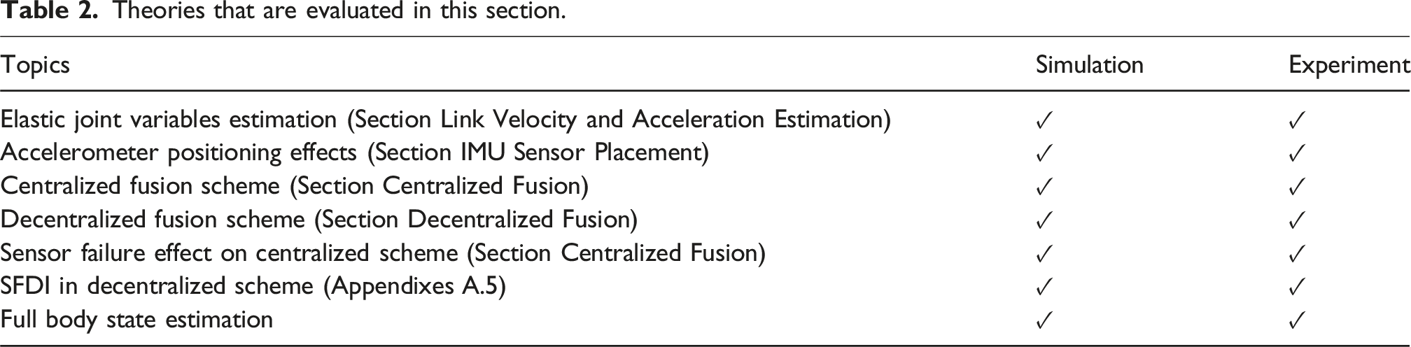
Simulations

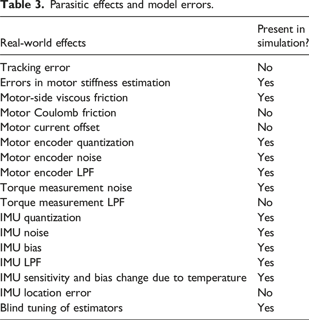
The simulation results in this section are reported in three stages. First, the results from Section IMU Sensor Placement, where we showed that the farther an IMU is from the rotation axis, the more information it contributes to the estimator, are evaluated. Moreover, the estimation accuracy of different local estimators is compared against centralized and decentralized fusion schemes, introduced in Section Multi-Sensor Fusion. The purpose of this section is to compare the estimation accuracy based on the accelerometer distance from the rotation axis when no sensor failure occurs. Subsequently, in the second stage, the two multi-sensor fusion methods are compared for different sensor failure scenarios. Lastly, multiple sensor failures occur within one simulation to evaluate the robustness of the SFDI algorithm. Prior to reporting the results, the simulation properties are summarized below.

Parasitic effects and model errors

In order to standardize the simulation evaluation, different real-world and parasitic effects as well as model mismatches are included in the calculations. Table 3 gives an overview of these effects, which are detailed in the following. LPF stands for low-pass filter in this table.The manipulator joint dynamics with joint damping, stiffness, as well as viscous friction are simulated according to equation (3). ⁵ The linear viscous friction model is

${\mathit{\tau }}_{\text{f}}={\mathit{F}}_{\mathrm{\theta }}\dot{\mathit{\theta }},$

(52)

with F _θ being the diagonal motor-side viscous coefficients matrix. The stiffness matrix in the joint dynamics model is of the form

${\mathit{K}}_{\text{J}}\sim \mathcal{N}({\widehat{\mathit{K}}}_{\text{J}},0.1{\widehat{\mathit{K}}}_{\text{J}}),$

(53)

where ${\widehat{\mathit{K}}}_{\text{J}}=\text{diag}\{{\widehat{K}}_{\text{J},1},\cdots {\widehat{K}}_{\text{J},7}\}\in {\mathbb{R}}^{7\times 7}$ denotes the joint stiffness used in the estimator measurement functions and $\mathcal{N}(\cdot )$ represents the normal distribution. The identification of the joint stiffness ${\widehat{\mathit{K}}}_{\text{J}}$ is based on well-established methods commonly applied in robotics, such as those found in SEA/VSA design literature and works like Albu-Schäffer (2002). For the sake of simplicity, the system is controlled via inverse dynamics control (Wankyun Chung and Hsu, 2008). However, any other suitable controller may be used as well. The simulated encoder is a 12-bit digital sensor whose three least significant bits (LSBs) are affected by noise. The quantization effects and an LPF are modeled for the simulated encoder. The LPF has a cutoff frequency of 300 Hz and attenuates high-frequency sensor noise. The IMUs are modeled based on the Bosch BMI055 (Bosch, 2014) with all parasitic effects such as noise, bias, quantization and sensitivity and bias change due to temperature. The temperature profile swings between 15°C and 40°C in a sinusoidal wave and affects the sensor drift and sensitivity in the simulation, based on the statistical relationships provided in the datasheet. Moreover, according to the datasheet, the noise power spectral density is 150 μg $/\sqrt{\text{Hz}}$ for accelerometers and 0.014°/s $/\sqrt{\text{Hz}}$ for gyroscopes. The full scale range is chosen 1 g for the accelerometer and 1000°/s for the gyroscope. Both sensors report the measurements in 12-bit resolution. Each link is equipped with three sensors (l = 3). The location of each set of sensors is ${}^{\text{i}}\mathit{X}_{\text{Set\hspace{0.17em}}1}={[00.050]}^T$ , ${}^{\text{i}}\mathit{X}_{\text{Set\hspace{0.17em}}2}={[0.10.150]}^T$ and ${}^{\text{i}}\mathit{X}_{\text{Set\hspace{0.17em}}3}={[0.30.30]}^T$ m w.r.t. their corresponding joint frame {i}. The estimators are blindly tuned, meaning that the accelerometer noise covariance matrices in the EKFs are equal for all sets of IMUs and independent of the sensor location. Therefore, the estimator bias introduced by tuning assumptions is minimized.

Table 3.

Parasitic effects and model errors.

Real-world effects	Present in simulation?
Tracking error	No
Errors in motor stiffness estimation	Yes
Motor-side viscous friction	Yes
Motor Coulomb friction	No
Motor current offset	No
Motor encoder quantization	Yes
Motor encoder noise	Yes
Motor encoder LPF	Yes
Torque measurement noise	Yes
Torque measurement LPF	No
IMU quantization	Yes
IMU noise	Yes
IMU bias	Yes
IMU LPF	Yes
IMU sensitivity and bias change due to temperature	Yes
IMU location error	No
Blind tuning of estimators	Yes

Reference trajectory

In both sections, the robot (all joints) is actuated to follow a 20-s excitation trajectory. This periodic Fourier-like trajectory (Swevers et al., 1997), defined as

$q_{\text{i}}(t)=q_{\text{i,0}}+\sum _{\text{r\hspace{0.17em}}=\hspace{0.17em}1}^R\frac{u_{\text{r},\mathrm{i}}}{r\omega }\sin (\mathrm{r}\omega t)-\sum _{\text{r\hspace{0.17em}}=\hspace{0.17em}1}^R\frac{v_{\text{r},\mathrm{i}}}{r\omega }\cos (\mathrm{r}\omega t),$

(54)

respects all robot joint limitations specified in the manufacturer datasheet. The number of harmonics in this trajectory is R = 5, and the fundamental frequency is ω = 0.1π rad/s. Table 4 lists the values of coefficients u_r,i and v_r,i and also the offset q_i,0 in radians. These parameters are obtained via an optimization routine, where robot joint and torque limits are provided as constraints. These coefficients are optimized to minimize uncertainty in identifying robot base parameters (Swevers et al., 1997). Therefore, this trajectory persistently excites the system across the entire bandwidth of interest, facilitating the evaluation of the estimator performance. Figure 7 depicts the 7-th joint velocity and acceleration excitation profiles as an example. For better visualization, only 7-th link estimation results are plotted in this section. These estimations are in fact, most prone to errors, due to the recursive nature of calculations.

Table 4.

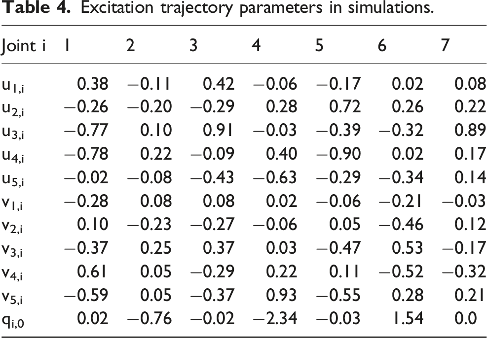
Excitation trajectory parameters in simulations.

Joint i	1	2	3	4	5	6	7
u1,i	0.38	−0.11	0.42	−0.06	−0.17	0.02	0.08
u2,i	−0.26	−0.20	−0.29	0.28	0.72	0.26	0.22
u3,i	−0.77	0.10	0.91	−0.03	−0.39	−0.32	0.89
u4,i	−0.78	0.22	−0.09	0.40	−0.90	0.02	0.17
u5,i	−0.02	−0.08	−0.43	−0.63	−0.29	−0.34	0.14
v1,i	−0.28	0.08	0.08	0.02	−0.06	−0.21	−0.03
v2,i	0.10	−0.23	−0.27	−0.06	0.05	−0.46	0.12
v3,i	−0.37	0.25	0.37	0.03	−0.47	0.53	−0.17
v4,i	0.61	0.05	−0.29	0.22	0.11	−0.52	−0.32
v5,i	−0.59	0.05	−0.37	0.93	−0.55	0.28	0.21
qi,0	0.02	−0.76	−0.02	−2.34	−0.03	1.54	0.0

Figure 7.

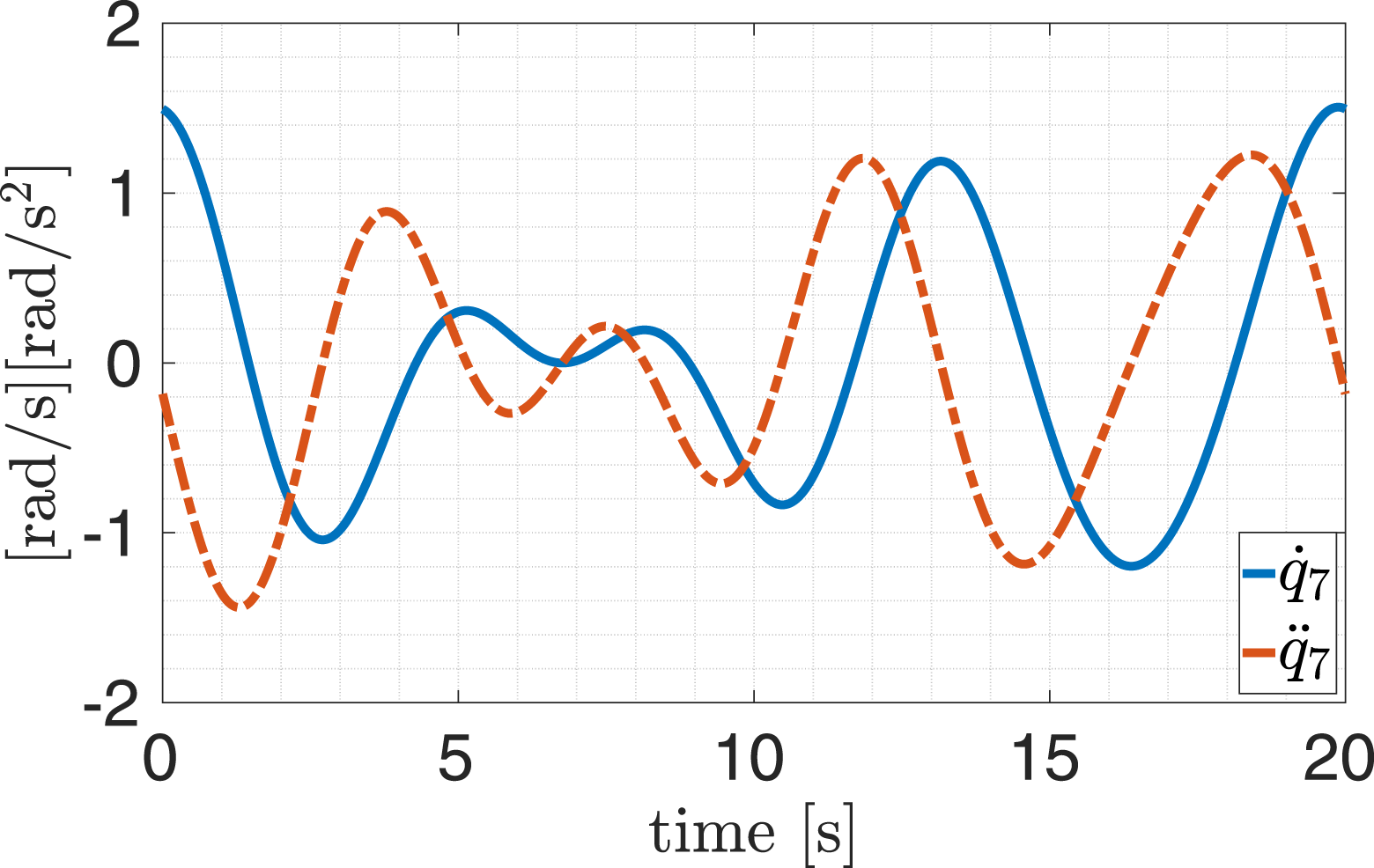
Velocity and acceleration reference trajectory in the seventh joint.

IMU location effect

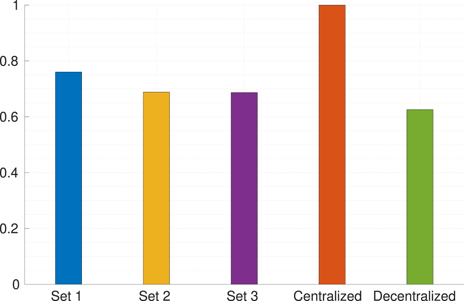
This section investigates the effect of the sensor location under blind tuning conditions. Section IMU Sensor Placement showed that the amount of information provided by an accelerometer is proportional to its distance from the link rotation axis. Let ${\mathit{e}}_{\text{j}}=\mathit{q}-{\widehat{\mathit{q}}}_{\text{j}}$ denote the estimation error of the j-th local estimator corresponding to the j-th set of sensors. Figure 8 compares the root mean square error (RMSE) of the estimated link acceleration in the local estimators as well as the decentralized and centralized fusion explained in Section Multi-Sensor Fusion. As expected from Section IMU Sensor Placement the third set, which is the farthest from the rotation axis, yields the smallest error among all local estimators. In the centralized estimator, the same tuning parameters as in the local estimators are used. Moreover, in the decentralized fusion, the weights are computed based on equation (47) in the decentralized fusion. Overall, decentralized fusion outperforms all estimations. As mentioned earlier, centralized fusion may be the optimal solution, for linear systems only. Since the system is governed by the nonlinear system equation (6), where the measurement covariance matrix is tuned equally for all IMUs irrespective of the corresponding accelerometer SNR, centralized fusion optimality is significantly compromised. In contrast, within decentralized fusion, the presence of each individual a posteriori error covariance matrix in the fusion law given by equation (48) helps to regulate the fused states more efficiently. For instance, when the third local estimator returns more accurate results, the a posteriori error covariance ( P _i,3) contains smaller elements. Therefore, the corresponding estimation receives higher significance (regardless of the tuning weight α_i,3) from the error covariance inverse matrix $({\mathit{P}}_{\text{i,}3}^{-1})$ in equation (48). This results in more accurate estimations in decentralized fusion. On the other hand, the centralized estimator not only produces less accurate estimations but also incurs high computation costs. Conversely, in decentralized fusion, the calculations are distributed among several remote agents. Thus, it requires less computation power in each individual estimator, including the central one. Figure 9 compares the estimator computation latency across methods. Decentralized refers to the central unit of decentralized fusion, where the fusion routine (equations (48) and (49)) are followed. Note that in this simulation, the SFDI algorithm runs in this central unit, which imposes some computation load on the decentralized scheme.

Figure 8.

RMSE $(\ddot{q})$ of each local estimator in rad/s².

Figure 9.

Normalized computation latency in different estimators.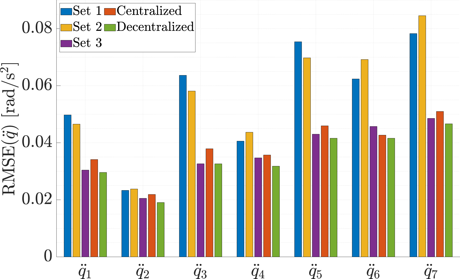

Fault detection and isolation

This section investigates the impact of sensor failure on the multi-sensor estimators. The second set of IMUs (spanning links 1 through 7) fails at t = 5 s and subsequently outputs pure noise. As shown in Figure 10(a), the decentralized method, which is equipped with failure detection and isolation mechanisms, adjusts the weights quickly (within 400 ms) after the failure occurs. For the centralized estimator, the error increases significantly after the failure.

Figure 10.

Fusion performance for link acceleration estimation in centralized 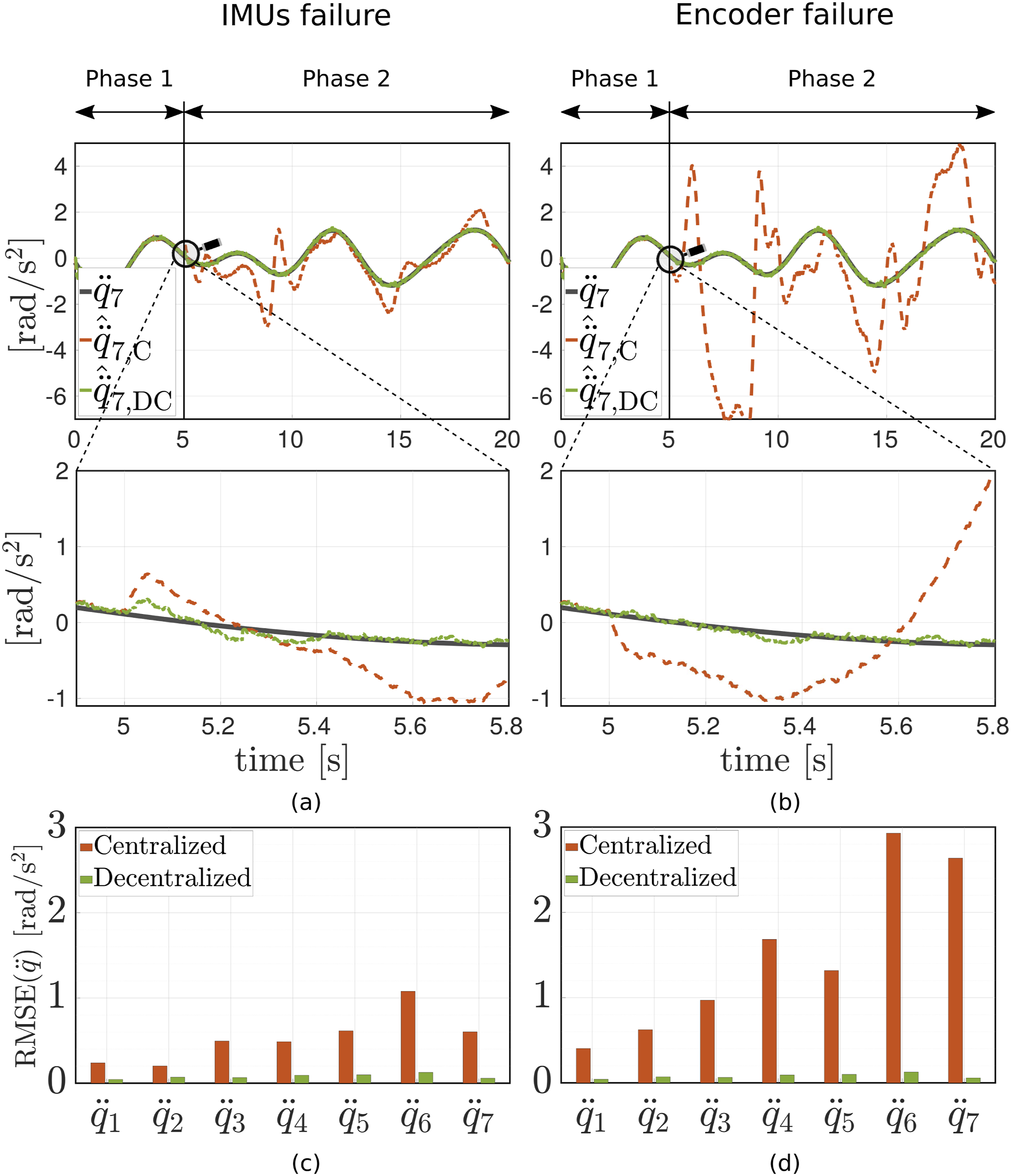$({\widehat{\ddot{q}}}_{\text{i},\mathrm{C}})$ and decentralized $({\widehat{\ddot{q}}}_{\text{i},\mathrm{D}\mathrm{C}})$ schemes. (a) Seventh link acceleration estimation, when all IMUs in the second set fail. (b) Seventh link acceleration estimation, when all encoders fail. (c) RMSE of acceleration estimation for all links, when all IMUs in the second set fail. (d) RMSE of acceleration estimation for all links, when all encoders fail. Phase 1: before sensor failure. Phase 2: after sensor failure.

Now, we compare the performance of the centralized and decentralized setups when the encoder in the seventh joint fails (see Figure 10(b)). As can be seen in the figure, the centralized fusion diverges further in this scenario. This is due to the fact that the encoder noise power is normally weaker than that of IMUs. Therefore, the corresponding measurement noise variance model in the EKF is smaller than that used for the IMUs. This means that the EKF trusts the encoder measurements more than IMU measurements. As a result, if an encoder fails in the centralized fusion method, the estimation errors will be more severe. The decentralized fusion method, on the other hand, has negligible error even with a reduced measurement function equation (95).

Figures 10(c) and (d) compare the RMSE $(\widehat{\ddot{q}})$ of centralized and decentralized fusion across all links, when IMUs and encoders fail, respectively.

Multiple asynchronous sensor failures

As explained in Appendixes A.5, the special weighting structure of covariance matrices in equations (46) and (48) keeps the system operational, even in an asymmetric sensor topology. In other words, the system can operate when multiple sensors fail. Therefore, in this section, we evaluate the SFDI performance when multiple sensors at different epochs fail. Seven sensor failure events are spread through an eighty-second simulation. The event epochs and the failing sensors are randomly picked. There are a total 35 sensors in this system and the failing ones (one-fifth of the total sensors) are chosen using MATLAB randi() syntax, which generates uniformly distributed random integer numbers. The failing times are selected using MATLAB rand() function. Table 5 summarizes these events. Figure 11 shows the seventh link acceleration estimation. As can be seen in the figure, the system is able to tolerate and isolate the sensor failures relatively competently until the sixth sensor fails (t = 43.12 s). These results confirm the reliability and robustness of the SFDI algorithm.

Table 5.

Summary of multiple asynchronous sensor failures.

Event Number	Epoch (s)	Sensor type	Joint number	Set number (IMUs only)
1	12.62	Torque	5	-
2	25.18	IMU	7	3
3	29.04	Encoder	6	-
4	36.52	Torque	2	-
5	38.46	IMU	6	1
6	43.12	IMU	3	3
7	61.71	IMU	3	2

Figure 11.

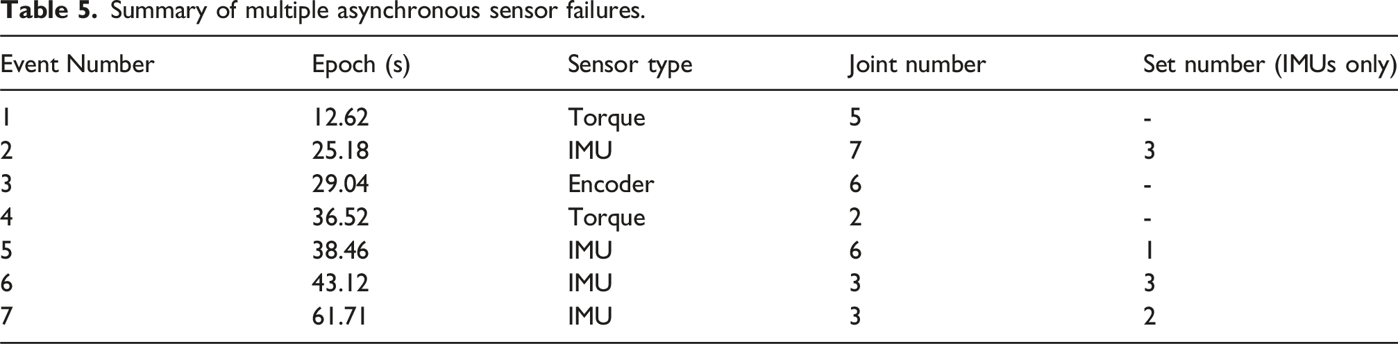
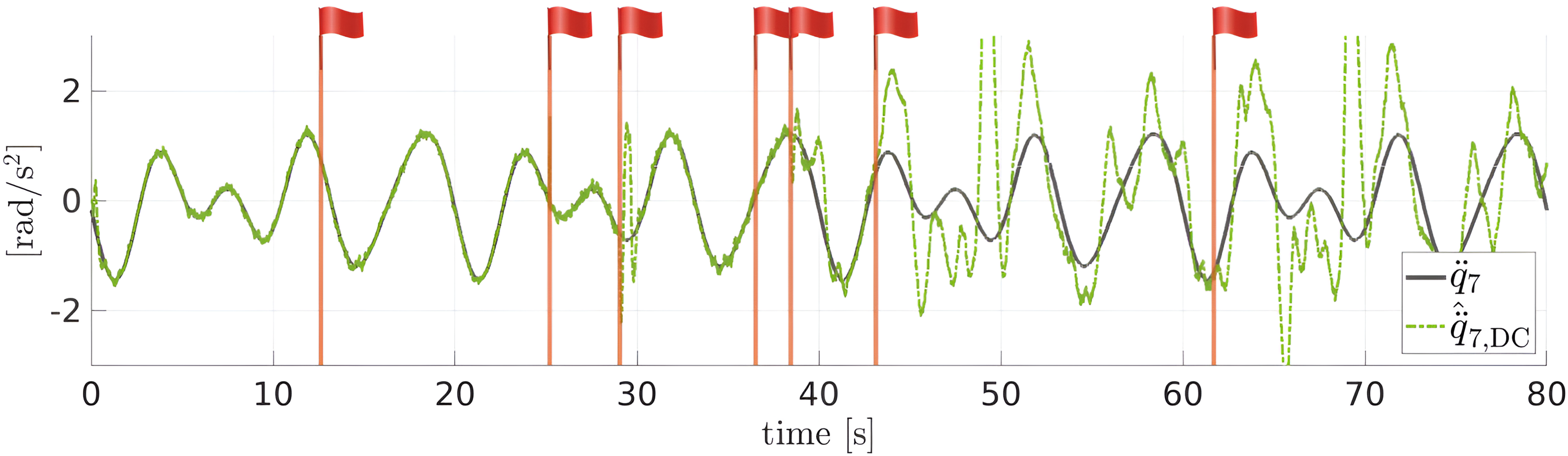
7-th joint acceleration estimation using decentralized fusion scheme when multiple sensors fail. Different events (sensor failures) are marked with flag symbols. Table 5 lists all the events.

Experiments

In this section, we evaluate our findings in a series of experiments with a 7-DoF robot arm, which aims to cover an extensive range of measures. Therefore, the experiment section is divided into three sub-sections: accelerometer SNR evaluation, multi-sensor fusion, and full link variable estimation. In the first section, we evaluate the theories discussed in Section Accelerometer Signal to Noise before fusing the sensors in a model-based estimator. Moreover, in multi-sensor fusion experiments, a one-link system is assumed by actuating one joint only. Furthermore, in full link variable estimation, each robot link is equipped with an IMU, and finally, link velocity and acceleration are estimated for all degrees of freedom. Note that to the best of the authors’ knowledge, no commercially available manipulator is currently equipped with installed IMUs so far. Thus, we manually install the sensors herein. The positions of the IMUs were measured using a highly accurate device, the FARO Laser Tracker X, with precision up to 10 μm. A detailed discussion of this technique can be found in Appendixe A.6, which was originally proposed in Baradaran Birjandi et al. (2019).

Accelerometer SNR evaluation

Before estimating the robot link velocity and acceleration, the accelerometer SNR problem and the proposed solutions in Section Accelerometer Signal to Noise are tested. Initially, we evaluate the first method, where the distance from the rotation axis determines the associated SNR. In order to demonstrate this issue, we install two IMUs (S₁ and S₂) on the robot’s second link (see Figure 12(a)). S₁ is closer (4.7 cm) to the rotation axis, whereas S₂ is placed farther (8.9 cm) from it. In this experiment, the IMUs are ST LSM6DSOTR. The full scale is set to 2 g for the accelerometer and 125°/s for the gyroscope for maximum measurement sensitivity. Moreover, the data is transmitted unfiltered with 1 kHz sampling rate. The robot measurement data rate is also 1 kHz. The second link is actuated to follow an excitation trajectory while the other links remain at rest. The clean signals ${}^2\mathit{a}_{S_1}$ and ${}^2\mathit{a}_{S_2}$ ( ${}^2\mathit{a}_{S_{\mathrm{1,2}}}$ in brief) are estimated via

${}^2\mathit{a}_{S_{\mathrm{1,2}}}=\left(\begin{array}{c}\hfill 0\hfill \\ \hfill 0\hfill \\ \hfill {\ddot{q}}_2\hfill \end{array}\right)\times {}^2\mathit{X}_{S_{\mathrm{1,2}}}+\left(\begin{array}{c}\hfill 0\hfill \\ \hfill 0\hfill \\ \hfill {\dot{q}}_2\hfill \end{array}\right)\times \left(\begin{array}{c}\hfill 0\hfill \\ \hfill 0\hfill \\ \hfill {\dot{q}}_2\hfill \end{array}\right)\times {}^2\mathit{X}_{S_{\mathrm{1,2}}},$

(55)

with ${}^2\mathit{X}_{S_{1\text{,}2}}$ being the sensor positions in the second link frame. Note that in order to have comparable results, all measurements and clean signals are rotated to the second link frame {2}. The link velocity ${\dot{q}}_2$ and acceleration ${\ddot{q}}_2$ in equation (55) are computed based on the numerical differentiation of the encoder output. In order to mitigate noise and potential phase shifts, the signal is filtered via lag-free filtering. As can be seen in Figures 12(b) and (c), compared to S₁, the signal amplitude and consequently its power increase in S₂ output. ${}^2\mathit{a}_{S_1}+N$ and ${}^2\mathit{a}_{S_2}+N$ denote the accelerometer S₁ and S₂ measurements (polluted by noise N) in the figures, respectively. Note that as the motion is planar, only two axes are visualized in these figures. The SNR associated with S₁ is 7.9 and to S₂ is 13.9.

Figure 12.

The experiments for evaluating the proposed solutions to the accelerometer SNR problem (see Section. Accelerometer Signal to Noise). (a) The robot’s second link is equipped with two IMUs. One IMU (S₁) is closer to and the other one (S₂) is farther from the link rotation axis. (b) The accelerometer S₁ measurement and the corresponding clean signal. The SNR is relatively low for this sensor. (c) The accelerometer S₂ measurement and the corresponding clean signal. The SNR improves for this sensor. (d) The robot’s seventh link is equipped with four IMUs. (e) The accelerometer S₁ measurements with relatively high noise power. (f) The fused measurement with relatively lower noise power.

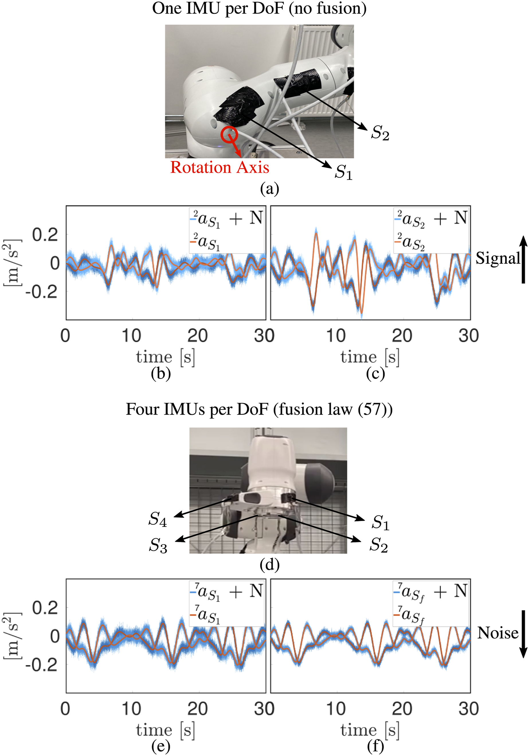
In the next experiment, we evaluate the second approach proposed in Section Accelerometer Signal to Noise. For this, we install four IMUs on the robot’s seventh link (see Figure 12(d)) and move the seventh link only along an excitation trajectory. In order to have a unified and comparable solution, the accelerometer measurements are projected to the sensor S₁ location ${}^7\mathit{X}_{S_1}$ via

$\begin{array}{ll}\hfill & {}^{\mathrm{7}}\mathit{a}_{S_{1\leftarrow \mathrm{i}}}={}^{\mathrm{7}}\mathit{R}_{S_i}{}^{S_i}\mathit{a}_{S_{\text{i}}}+\left(\begin{array}{c}\hfill 0\hfill \\ \hfill 0\hfill \\ \hfill {\ddot{q}}_7\hfill \end{array}\right)\times \left({}^{\mathrm{7}}\mathit{X}_{S_1}-{}^{\mathrm{7}}\mathit{X}_{S_{\text{i}}}\right)\hfill \\ \hfill & +\left(\begin{array}{c}\hfill 0\hfill \\ \hfill 0\hfill \\ \hfill {\dot{q}}_7\hfill \end{array}\right)\times \left(\begin{array}{c}\hfill 0\hfill \\ \hfill 0\hfill \\ \hfill {\dot{q}}_7\hfill \end{array}\right)\times ({}^7\mathit{X}_{S_1}-{}^{\mathrm{7}}\mathit{X}_{S_{\text{i}}}),\text{with\hspace{0.17em}}\mathrm{i}\in \{\mathrm{2,3,4}\}.\hfill \end{array}$

(56)

Here, ${}^7\mathit{a}_{S_{1\leftarrow \mathrm{i}}}$ denotes the transformed acceleration from sensor S_i location to that of sensor S₁ and ${}^7\mathit{R}_{S_{\text{i}}}$ rotates the accelerometer S_i measurement $({}^{S_{\text{i}}}\mathit{a}_{S_{\text{i}}})$ to the seventh link frame {7}. The clean signal is again computed similarly to equation (55). Except for one sensor ( $\approx 9$ cm) the distance from the accelerometers to the seventh link rotation axis is $\approx 4$ cm. However, we fuse the sensors blindly. In other words, irrespective of each individual sensor SNR, the fusion coefficients are equally distributed as

${}^7\mathit{a}_{S_{\text{f}}}=\frac{1}{4}{}^7\mathit{a}_{S_1}+\frac{1}{4}{}^7\mathit{a}_{S_{1\leftarrow 2}}+\frac{1}{4}{}^7\mathit{a}_{S_{1\leftarrow 3}}+\frac{1}{4}{}^7\mathit{a}_{S_{1\leftarrow 4}}.$

(57)

Here, ${}^7\mathit{a}_{S_{\text{f}}}$ is the fused measurement. As can be seen in Figures 12(e) and (f), the noise power in sensor S₁ (SNR = 10.5) is considerably reduced in the fused measurement S _f (SNR = 14.5).

Multi-sensor fusion

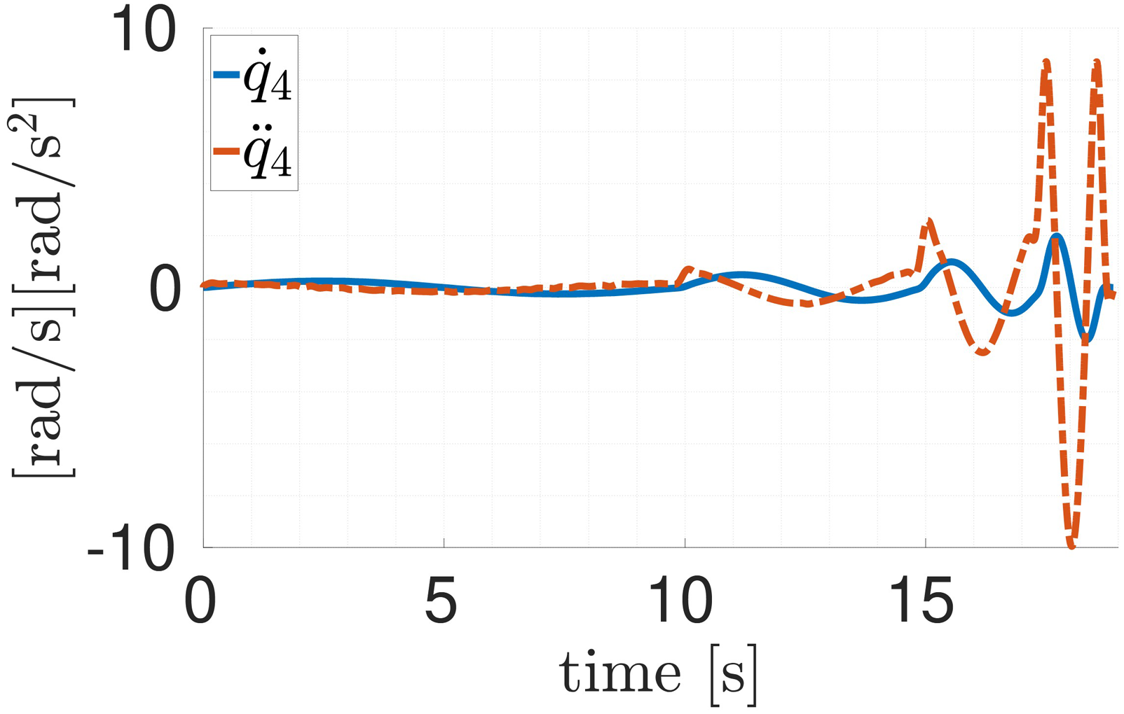
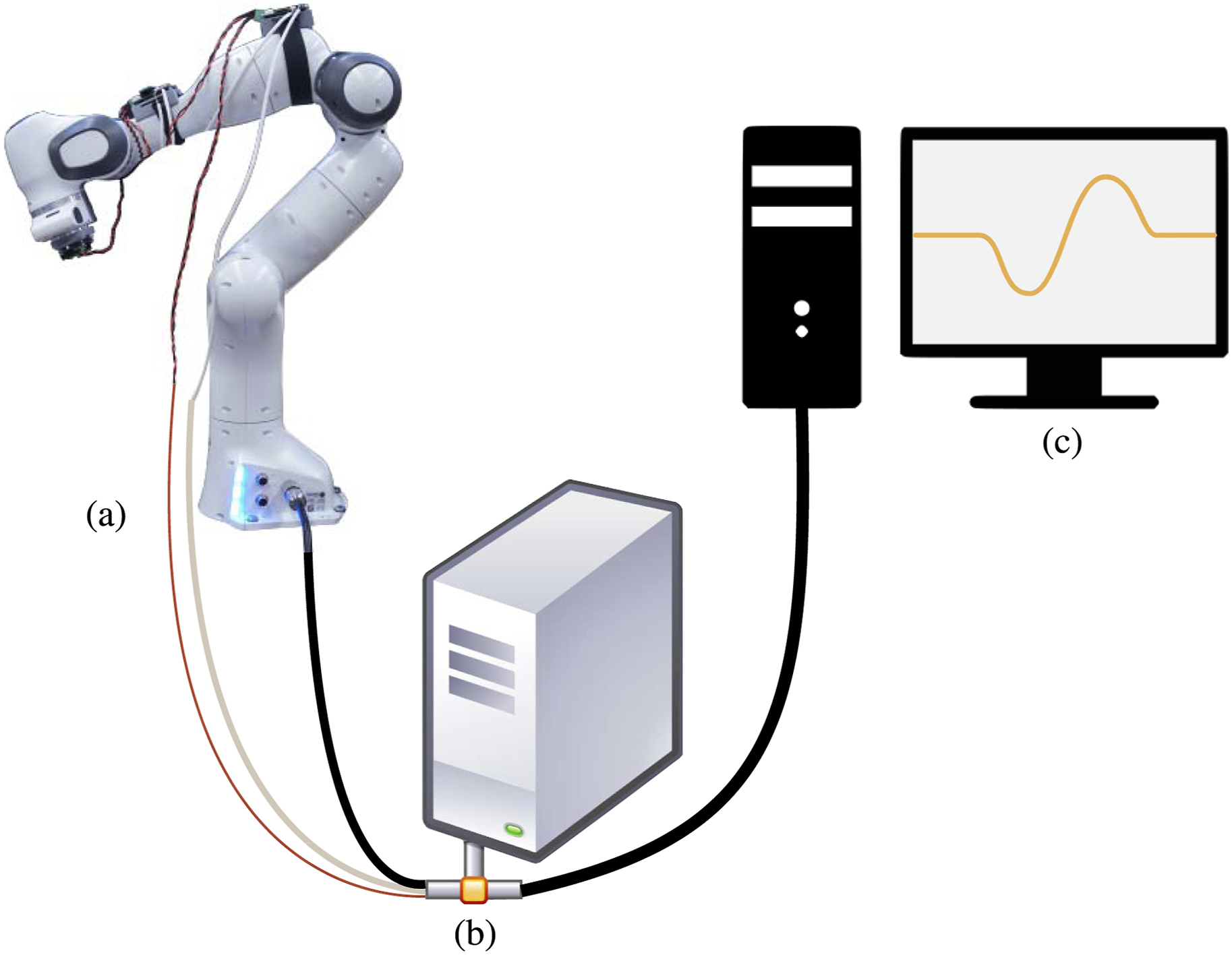
In this setup, three IMUs are mounted at known locations on the robot body (Figure 13). The IMUs for this experiment are Bosch BMI055. The measurement and robot sampling frequency is 1 kHz. The internal filters of the IMUs are not used, which in turn allows raw data streaming. For the maximum-sensitivity measurements, the range is set to 2 g for the accelerometer and 125°/s for the gyroscope. The fourth joint is actuated in this experiment. Accordingly, the first IMU is mounted close (close setup) to the fourth joint. The second one is in the middle of the fifth link (middle setup). The third IMU is attached to the robot end-effector (EE setup). Different sensor locations are ultimately meant to resemble a multi-sensor setup. The distance of each sensor from the rotation axis is approximately 18 cm for the close IMU, 35 cm for the middle IMU, and 50 cm for the end-effector IMU. In order to provide an extreme showcase, the latter is relatively far from the rotation axis. Please note that all robot links have to be equipped with IMUs in order to be able to fully actuate the robot manipulator and estimate the link variables. This assumption, however, falls short in the current setup, where one link is considered to be actuated. As a result, we repeat the scenarios in Section Simulations using a different trajectory. The trajectory is a sinusoidal motion in the fourth joint with different velocities. Different velocities let us evaluate our method bandwidth. Figure 14 depicts the ground truth trajectory. In order to generate the ground truth trajectory, the motor-side position θ₄ and the joint torque τ₄ are measured. Consequently, the link-side position q₄ is computed via equation (3). Here, the joint stiffness K_J,4 ≈ 10000 Nm/rad is estimated offline. The link-side position is subsequently differentiated and filtered via zero-phase filtering techniques to derive the link-side velocity and acceleration (see Figure 14). In order to keep the results as unbiased as possible, two assumptions are considered in the experiments. Local estimators are tuned blindly, meaning that the measurement covariance matrices in equation (6) are the same for all three IMUs, regardless of their distance from the rotation axis. This distance affects the accelerometer SNR (see Section Accelerometer Signal to Noise). Also, the weight (α_close, α_middle, and α_EE) in the decentralized fusion (48) is 1/3 for each local estimator. Figure 15 depicts the experimental setup. Data acquisition (DAQ) receives the robot proprioceptive sensor and IMU readings. In order to make the experiment more realistic, decision-making and fault isolation, as well as fusion, are done on another processor. As the local estimators run on the DAQ system, the communication between the DAQ system and the fusion unit requires minimum bandwidth in the decentralized fusion. On the other hand, all unprocessed measurements are directly sent to the second processor in centralized fusion.

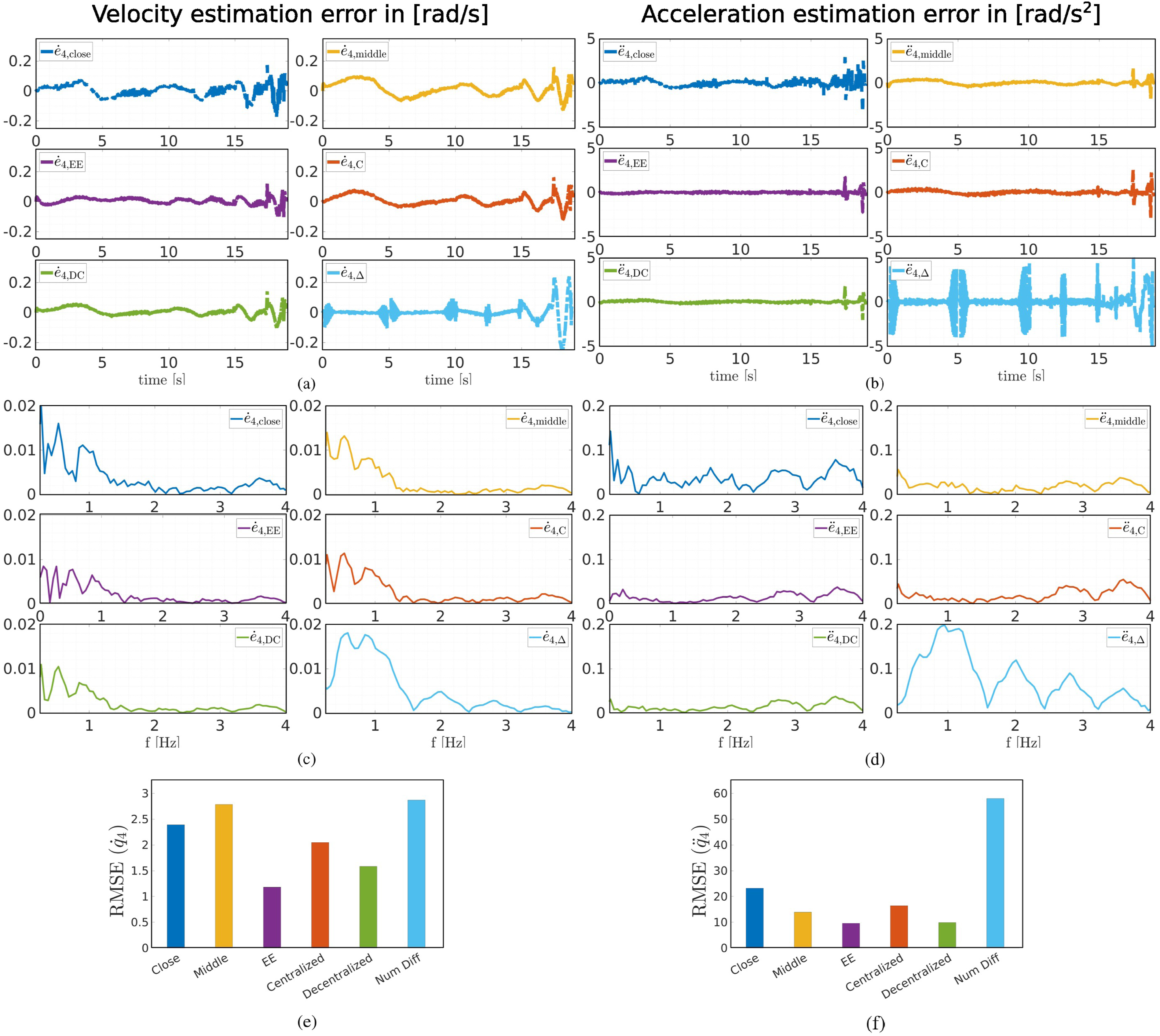
In the first part of the experiments, we compare the estimation performance of the centralized and decentralized methods in the absence of sensor failures. Figure 16 summarizes the experiment results in terms of estimation error in time domain (a) and (b), estimation error in frequency domain (c) and (d) and RMSEs (e) and (f) for both link velocity and acceleration. Frequency response helps to better analyze the estimation performance over the spectrum of the trajectory. In general, this figure shows that the estimation error in the EE setup is remarkably smaller than in the close setup. This confirms our findings in Section Link Velocity and Acceleration Estimation. Herein, ${\dot{e}}_{4,\mathrm{\Delta }}$ and ${\ddot{e}}_{4,\mathrm{\Delta }}$ refer to link velocity and acceleration error signals, respectively, which are obtained by numerically differentiating the computed link-side position signal and filtering it. Moreover, Num Diff refers to numerical differentiation with filtering in Figures 16(e) and (f). The low pass FIR filter is of order 50 and the cutoff frequency 10 Hz. ${\dot{e}}_{4,\mathrm{\Delta }}$ is mainly caused by the effect of quantization in motor-side position measurements and also the filter phase shift. The relatively large error of this method compared to the worst estimator (close) means that numerical differentiation is not a viable solution to obtain link-side acceleration in this one-link system. Moreover, the system cannot tolerate sensor failures due to a lack of sensor redundancy. This matter is considered for the estimators in the next section. According to Figure 16, decentralized fusion with equal weights (α_close = α_middle = α_EE = 1/3) for local estimators has a slightly better performance compared to the centralized fusion. This is due to the fact that fusion law (48) regulates the fused state based on the a posteriori error covariance matrix. In other words, the most accurate estimations (here, the EE local estimator) contribute most to the fused state. Both fusion methods can improve by tuning the accelerometer covariance in equation (6) and also the decentralized weights (α_close, α_middle, and α_EE) as explained in Section Decentralized Fusion.

Figure 13.

IMU setup for investigating (1) IMU location effect on link velocity and acceleration estimation accuracy and (2) sensor failure detection and isolation performance.

Figure 14.

4-th link velocity and acceleration reference trajectory.

Figure 15.

Experimental setup for estimating link velocity and acceleration of the system via centralized and decentralized architectures. (a) The robot is equipped with three IMUs, namely, close, middle, and EE IMUs. (b) DAQ system. (c) Fusion unit (49). Note that the DAQ system (b) is used as the local estimator in decentralized fusion. (b) is the central fusion unit (42) and (43) in centralized fusion architectures, as well. The local estimation data is sent to another processor (c) for final estimation in a decentralized fusion scheme.

Figure 16.

4-th link variables estimation errors. 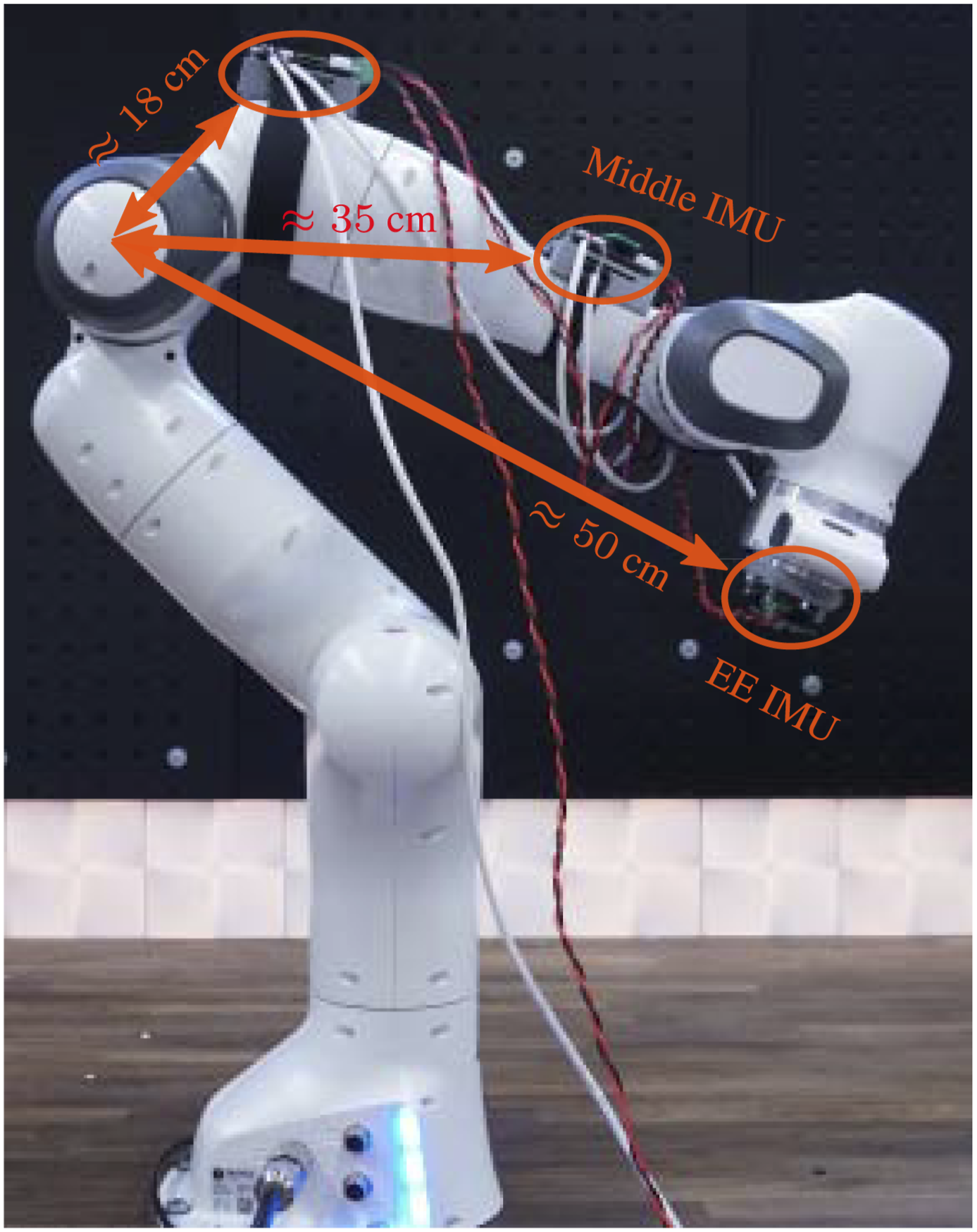${\dot{e}}_{4\text{,close}}$ $({\ddot{e}}_{4,\text{close}})$ , ${\dot{e}}_{4,\text{middle}}$ $({\ddot{e}}_{4,\text{middle}})$ , and ${\dot{e}}_{4,\text{EE}}$ $({\ddot{e}}_{4,\text{EE}})$ refer to the link velocity (acceleration) estimation error in the close, middle, and EE local estimators, respectively. Estimation errors in the centralized and decentralized estimators are indicated by C and DC, respectively. (a) Link velocity estimation error in the time domain for different methods. (b) Link acceleration estimation error in the time domain for different methods. (c) Link velocity estimation error in the frequency domain for different methods. (d) Link acceleration estimation error in the frequency domain for different methods. (e) RMSE of the estimated link velocity for different methods. (f) RMSE of the estimated link acceleration for different methods.

Now, the performance of the estimators when a sensor fails is investigated. The same trajectory as in the previous section is used here. The output of the failing sensor is set to zero at t = 12 s. When a sensor fails in this experiment, its output becomes zero.

In the first scenario, the close IMU fails. Figures 17(a) and (b) depict the velocity and acceleration estimation results in this scenario, respectively. The centralized method’s link velocity and acceleration show relatively large errors after the sensor failure. The jump in the acceleration estimation after the close IMU failure results in an offset in the estimated velocity signal. This offset makes the centralized estimation unreliable. Decentralized fusion, on the other hand, shows almost no divergence in this scenario (RMSE $({\widehat{\dot{q}}}_{4,\text{DC}})=1.5$ rad/s, RMSE $({\widehat{\ddot{q}}}_{4,\text{DC}})=9.2$ rad/s²). The reason that RMSE $({\widehat{\ddot{q}}}_{4,\text{DC}})$ decreased compared to the previous experiment (RMSE $({\widehat{\ddot{q}}}_{4,\text{DC}})=9.9$ rad/s²), where no sensor failure occurred, is that the decentralized weights are only distributed among the more accurate IMUs (middle and EE IMUs) after the incident.

Figure 17.

Fourth link variables estimation in time when different sensors fail. (a), (b) The close IMU fails at t = 12 s. (c), (d) The EE IMU fails at t = 12 s. (e), (f) The encoder fails at t = 12 s.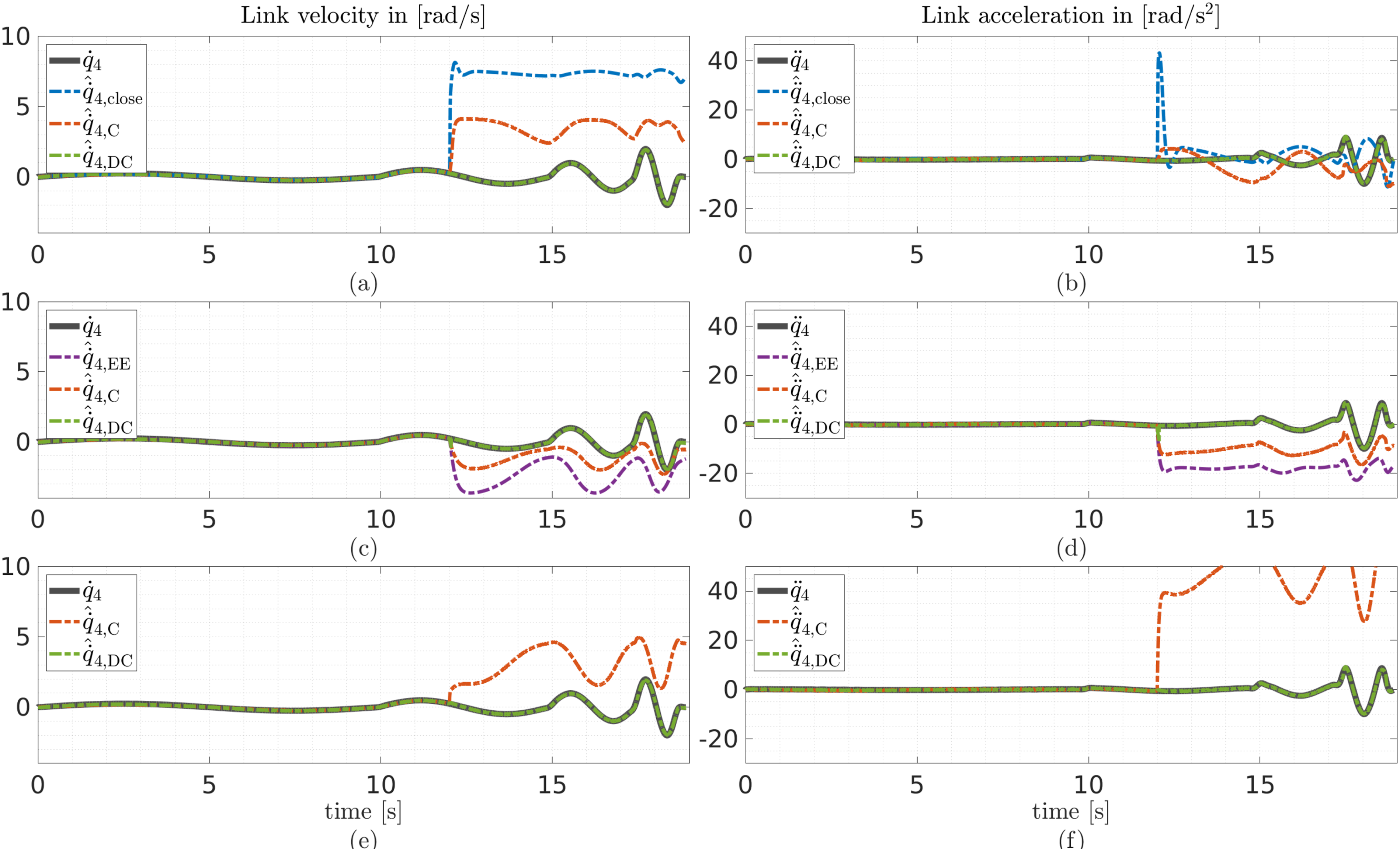

The EE IMU fails at t = 12 s in the next scenario. The link velocity and acceleration results are presented in Figures 17(c) and (d), respectively. As can be seen, the centralized method will again not be able to estimate properly after the failure. Furthermore, the link acceleration (RMSE $({\widehat{\ddot{q}}}_{4,\text{DC}})=16$ rad/s²) and velocity (RMSE $({\widehat{\dot{q}}}_{4,\text{DC}})=2.3$ rad/s) degrade about two times in the decentralized fusion, as the most accurate local estimator (EE) is bypassed. However, the estimations are still relatively accurate.

In the last scenario, the encoder fails at t = 12 s (Figures 17(e) and (f)). The performance degradation is again significant in the centralized fusion. Decentralized fusion shows promising estimation results in an encoder failure scenario with RMSE $({\widehat{\dot{q}}}_{4,\text{DC}})=1.6$ rad/s and RMSE $({\widehat{\ddot{q}}}_{4,\text{DC}})=10.4$ rad/s².

This section showed that numerical differentiation is not a proper approach to compute link-side velocity and acceleration for a one-link system. This is because the small quantization effects and/or measurement noise are enormously amplified after differentiation. However, using IMUs for this one-link robot makes link variable estimation possible. Fusing these sensors with the robot’s proprioceptive measurements improves the estimation accuracy and brings robustness to the decentralized scheme, where SFDI can be implemented. This entails, however, an extra initial effort to set up distributed systems when designing decentralized fusion. In return, and in comparison with the centralized method, the decentralized system can tolerate multiple sensor failures in a run while consuming less computational power in each distributed unit. However, the main practical issue with IMUs is noise power and bias. These parameters are sometimes so volatile that it is impossible to tune the estimators. If one manages to obtain measurement covariance matrices based on large samples, the system can be tuned. Yet, the variables can easily drift due to temperature changes. This causes the estimation error to grow larger with time. In other words, the estimators should be calibrated before every run, which prevents the method from becoming a general industrial solution. This method may be useful in the future, when the IMU noise power, bias, and drift are small and deterministic.

Full link variable estimation

In this section, each robot link is equipped with an IMU, enabling us to estimate the kinematics of all robot DoFs. We initially explain the approaches to obtain the ground truth signal. Subsequently, the necessity of using an excitation trajectory in the experiments, as well as the implementation, is outlined. As the robot is fully equipped with IMUs, the method for estimating the Cartesian kinematics is investigated. Finally, we evaluate estimator equation (6) with full-body actuation.

Ground truth

In order to provide the ground truth we mainly use two methods in this section. In the first method, we use the FARO Laser Tracker X, which uses laser technology to measure points. The device sends a beam to a spherically mounted retroreflector (SMR) at the point of measurement. The SMR reflects the beam to the laser tracker, and thus, the coordinates of the SMR in the laser tracker frame can be obtained. The device benefits from advanced technologies that make accurate measurements (up to 10 μm) with high sampling rates (up to 10 kHz) possible. Moreover, the device can follow the SMR in the whole three-dimensional workspace. However, the device stops following as soon as the SMR deflects the beam along its trajectory. Also, the device is unable to follow rapid SMR motions. Therefore, an alternative method to provide the ground truth is also used, which is based on the lag-free filtering of the encoder measurements.

Due to the limitations of the laser tracker, we propose two types of trajectories: slow and full dynamics motions. In the slow dynamics motions, the robot moves slowly. Also, the orientation of the SMR is kept relatively constant such that it reflects the laser beam to the tracker along its trajectory. Therefore, the laser tracker can follow the SMR and provide the ground truth in slow dynamics trajectories. However, these motions are not extensive, and therefore, the true bandwidth of the system is not evaluated. On the other hand, the full dynamics motion, which is intrinsically a persistently exciting trajectory, covers the whole spectrum of the robot bandwidth. Since the laser tracker cannot follow this trajectory, the ground truth is only computed based on the alternative method.

In these sets of experiments, the robot is equipped with one IMU per link. The system sampling rate is 1 kHz. The acceleration and angular velocity data are acquired using seven on-board STMicroelectronics LSM6DSOTR IMU sensors. The full-scale range and the Output Data Rate of the accelerometer and gyroscope sensors are set to 2 g and 6.67 kHz, and 2000°/s and 6.67 kHz, respectively. All IMU internal filters are deactivated. The use of high-bandwidth RS485 transceivers between the IMUs and the main board allows for fast and robust communication. The onboard microcontroller is capable of handling up to eight sensors and six channels (three for accelerometer and three for gyroscope) per sensor at 10 kS/s per channel. Consequently, the data is sent (based on the Master request) via the EtherCAT bus at a 1 kHz sampling rate. A Control PC (x64) running an Ubuntu 20.04 real-time system hosts the EtherCAT Master using Etherlab. Finally, the data is recorded in real-time via MATLAB/Simulink on the control PC. Another real-time system provides the robot with the desired velocity trajectory. For slow dynamics motions, the laser tracker follows and registers the SMR trajectory, attached to the robot end-effector, with 1 kHz sampling rate. The experimental setup is depicted in Figure 18.

Figure 18.

The schematic of the experimental setup.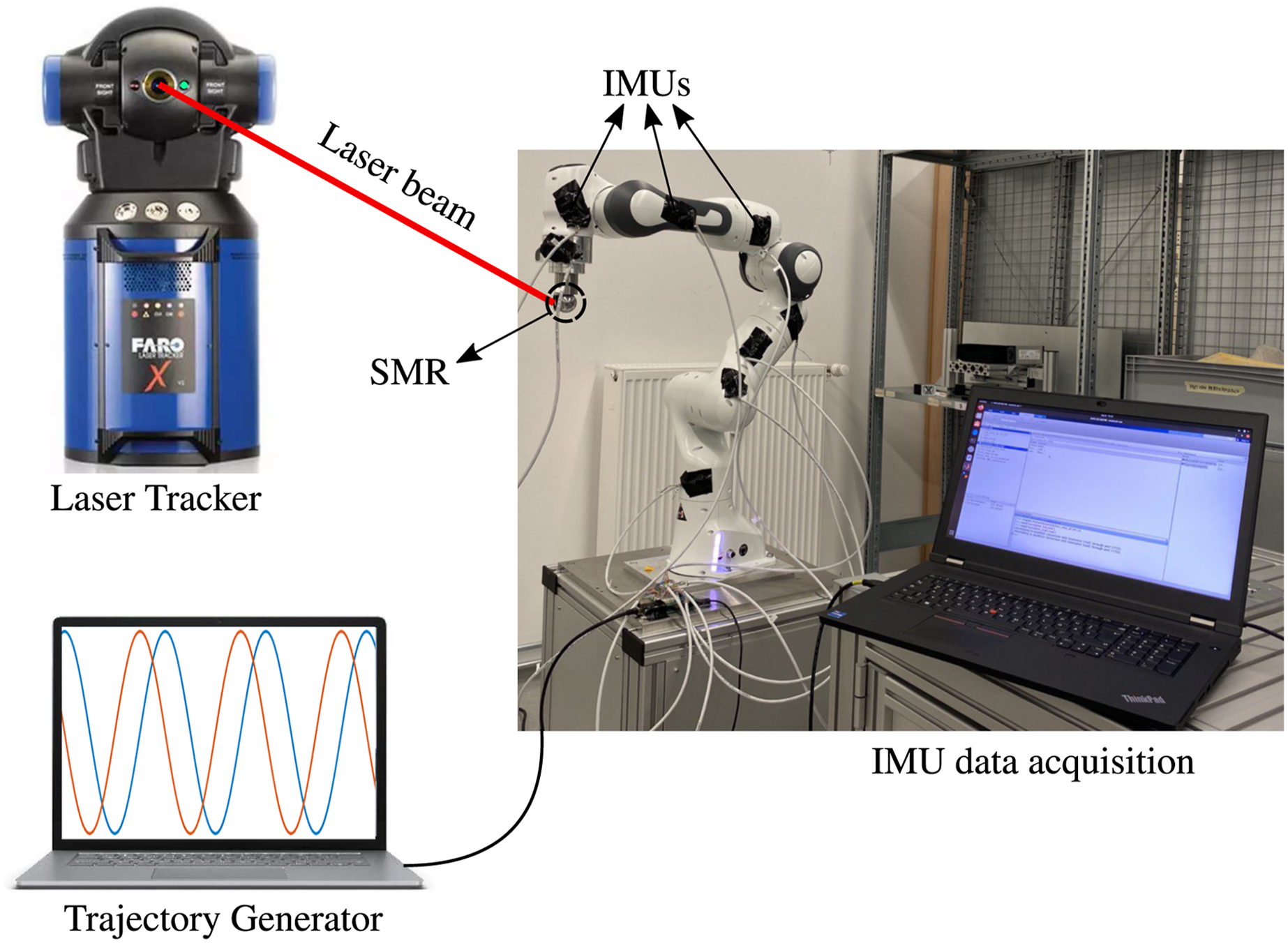

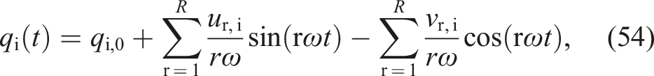
Excitation trajectory

In order to fully evaluate the bandwidth of the estimator equation (6), we move the robot in a persistently exciting trajectory in full-dynamics motions (see Section Full Link Variable Estimation). These trajectories are conventionally used for estimating the robot manipulators’ dynamics (see, e.g., Atkeson et al. (1986)). The robot is actuated to follow a 30-second excitation trajectory. The trajectory is formulated according to equation (54). The number of harmonics in this trajectory is R = 60, and the base frequency is ω = 2π/30. These parameters are obtained via an optimization routine, where robot joint and torque limits are provided as constraints. These coefficients are optimized for minimal uncertainty in identifying robot base parameters (Swevers et al., 1997). Therefore, this trajectory persistently excites the system along the whole bandwidth and subsequently evaluates the estimator equation (6) performance.

Slow dynamics motions

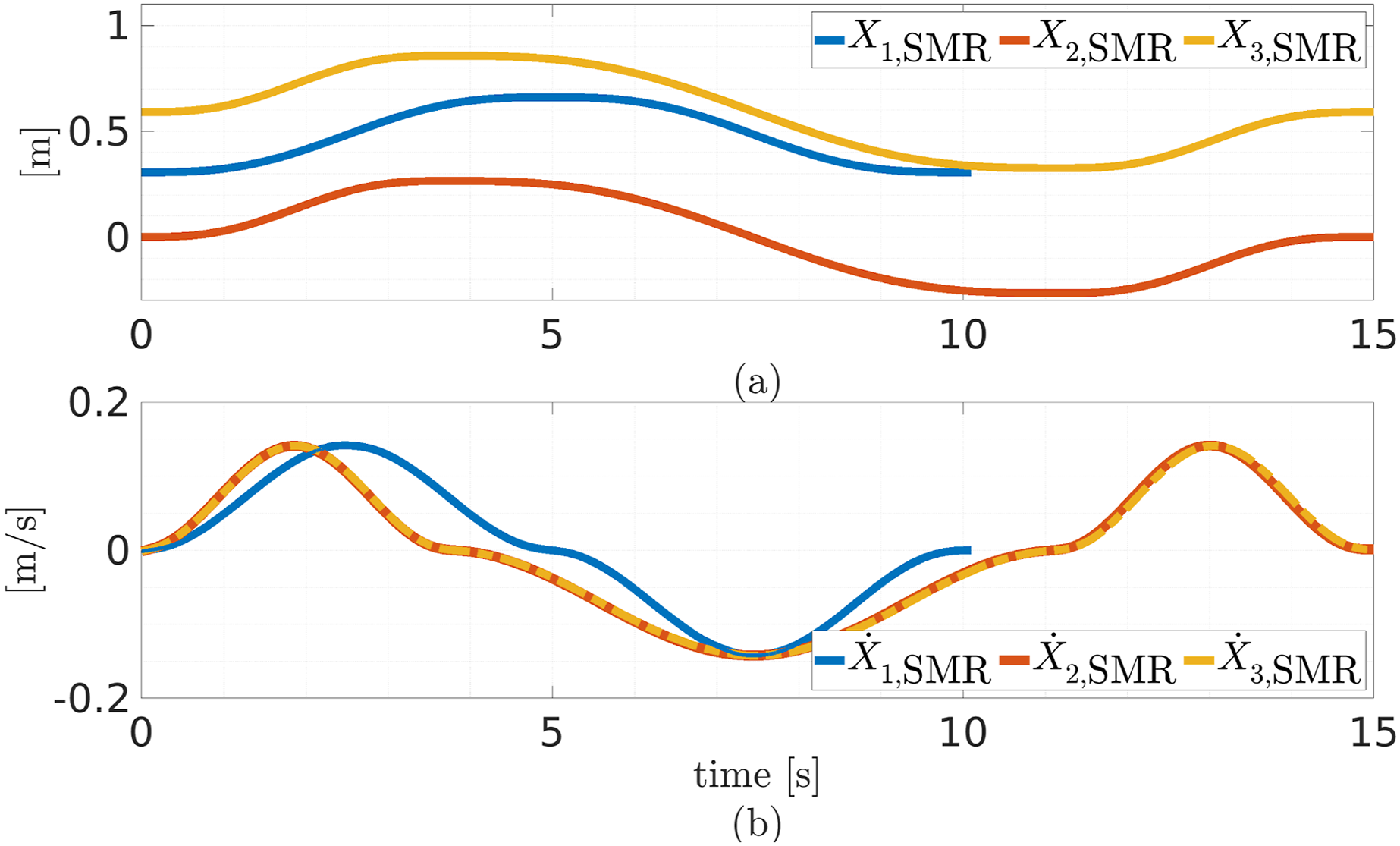
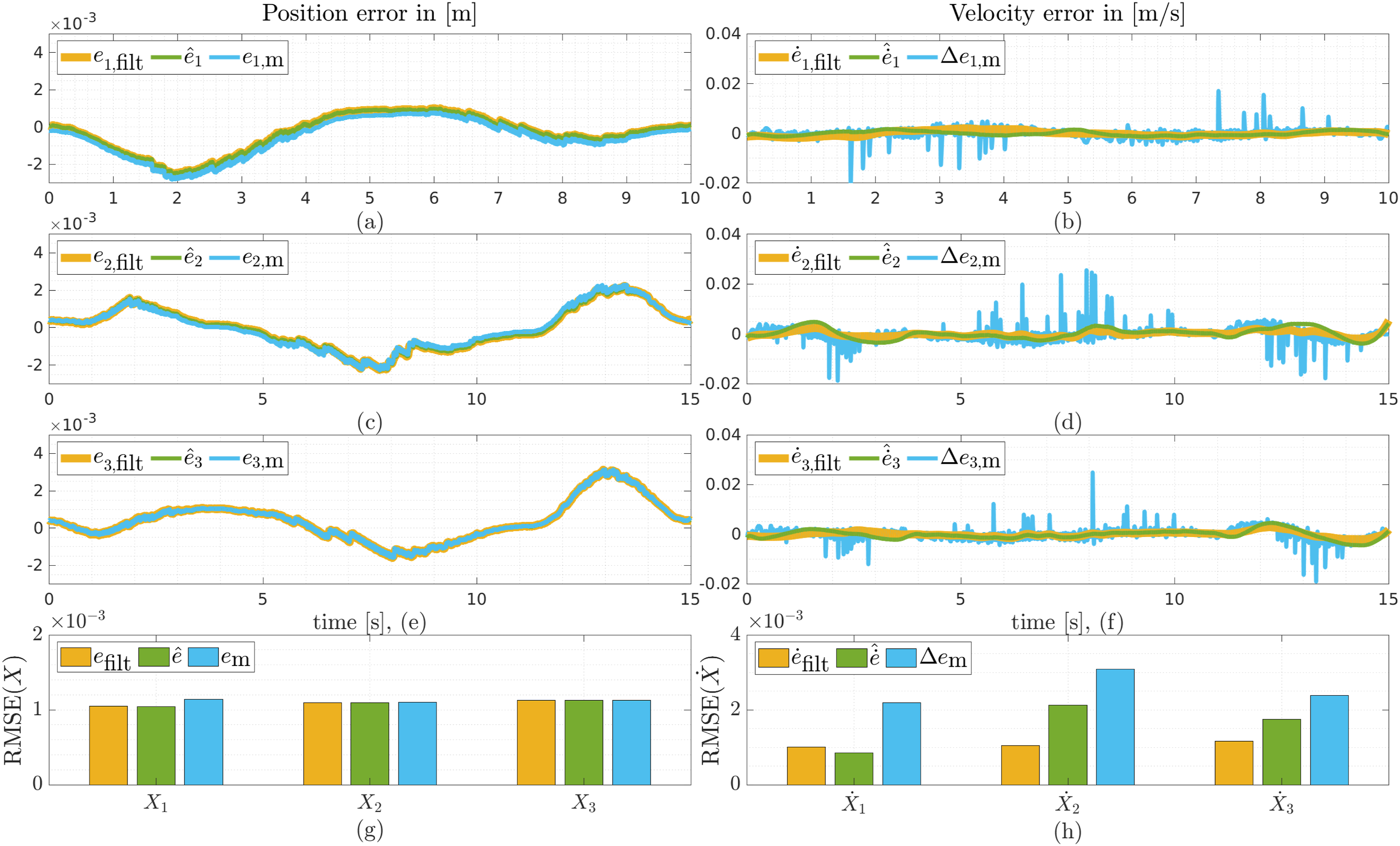
In these experiments, the robot moves along one Cartesian axis (three trajectories in total) in the robot base frame, at a time. The SMR moves along the robot base axes in three Cartesian trajectories (X₁, X₂, and X₃). Therefore, the laser tracker can follow the SMR attached to the robot end-effector. Figures 19(a) and (b) depict the position and velocity trajectories, respectively. In these figures, the ground truth X _SMR is the laser tracker signal, which is transformed to the robot base. The Cartesian position and velocity are estimated using forward kinematics based on the estimated link variables, as explained in Section Cartesian Position and Velocity Estimation. The results are reported in Figure 20. In the figure, the error signals are obtained via

$\begin{array}{ll}\hfill {\mathit{e}}_{\text{filt}}& ={\mathit{X}}_{\text{SMR}}-{\mathit{T}}_{\text{SMR}}({\mathit{q}}_{\text{filt}})={\mathit{X}}_{\text{SMR}}-{\mathit{X}}_{\text{filt}},\hfill \\ \hfill {\dot{\mathit{e}}}_{\text{filt}}& =\frac{\mathrm{\Delta }}{\mathrm{\Delta }t}{\mathit{X}}_{\text{SMR}}-\frac{\mathrm{\Delta }}{\mathrm{\Delta }t}{\mathit{X}}_{\text{filt}},\hfill \\ \hfill \widehat{\mathit{e}}& ={\mathit{X}}_{\text{SMR}}-{\mathit{T}}_{\text{SMR}}(\widehat{\mathit{q}}),\hfill \\ \hfill \widehat{\dot{\mathit{e}}}& =\frac{\mathrm{\Delta }}{\mathrm{\Delta }t}{\mathit{X}}_{\text{SMR}}-{\mathit{J}}_{\text{SMR}}(\widehat{\mathit{q}})\widehat{\dot{\mathit{q}}},\hfill \\ \hfill {\mathit{e}}_{\text{m}}& ={\mathit{X}}_{\text{SMR}}-{\mathit{X}}_{\text{m}},\hfill \\ \hfill {\dot{\mathit{e}}}_{\text{m}}& =\frac{\mathrm{\Delta }}{\mathrm{\Delta }t}{\mathit{X}}_{\text{SMR}}-\frac{\mathrm{\Delta }}{\mathrm{\Delta }t}{\mathit{X}}_{\text{m}}.\hfill \end{array}$

(58)

Here, q _filt is the link position which is (lag-free) filtered. ${\mathit{T}}_{\text{SMR}}:{\mathbb{R}}^7\to {\mathbb{R}}^3$ is the forward kinematics function to the SMR position. Moreover, Δ X _SMR/Δt denotes numerical differentiation of the laser tracker signal, followed by lag-free filtering. The same lag-free filtering is conducted after numerical differentiation of X _filt (Δ X _filt/Δt). Furthermore, X _m is the SMR position in the robot base frame, measured by the robot interface. Its numerical differentiation Δ X _m/Δt is filtered by a second-order low-pass filter with a 20 Hz cutoff frequency. According to the RMSE( X ) (see Figure 20(g)) of the position, all methods generate relatively acceptable results. However, the RMSE $(\dot{\mathit{X}})$ (see Figure 20(h)) of the Cartesian velocity is, in general, more accurate ( $<1.1$ mm/s) when the link position is filtered via lag-free filtering. Therefore, this method can be safely used as the ground truth for a full dynamics motion experiment, where the laser tracker is technically not able to follow the robot. The RMSE $({\dot{\mathit{X}}}_1)$ in the proposed solution is relatively smaller than the other two trajectories. This confirms our findings in Baradaran Birjandi et al. (2022), where we showed that the proposed solution works properly as long as there are few discontinuities in the trajectory. Note that in the reference trajectories, we manually inserted acceleration discontinuities. Moreover, the proposed solution estimates the Cartesian velocity (RMSE $({\dot{\mathit{X}}}_{\mathrm{1,2,3}})$ $<1.8$ mm/s) more accurately compared to numerical differentiation of the measured position (RMSE $({\dot{\mathit{X}}}_2)$ up to 2.8 mm/s).

Figure 19.

Reference position (a) and velocity (b) trajectories in the robot base frame, in slow dynamics experiments. The robot follows one trajectory at a time. The trajectories contain acceleration discontinuities.

Figure 20.

The experiments for evaluating the proposed method for estimating Cartesian position and velocity (see Section Cartesian Position and Velocity Estimation) in slow dynamics motions. (a) The position error in the robot base X₁-axis, based on different methods. (b) The velocity error in the robot base X₁-axis, based on different methods. (c) The position error in the robot base X₂-axis, based on different methods. (d) The velocity error in the robot base X₂-axis, based on different methods. (e) The position error in the robot base X₃-axis, based on different methods. (f) The velocity error in the robot base X₃-axis, based on different methods. (g) RMSE of position for all trajectories. (h) RMSE of velocity for all trajectories.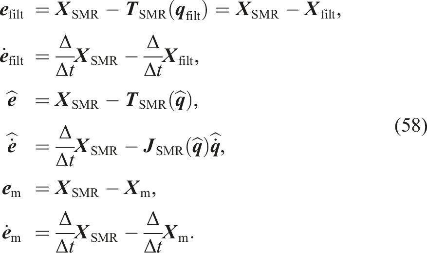

Full dynamics motions

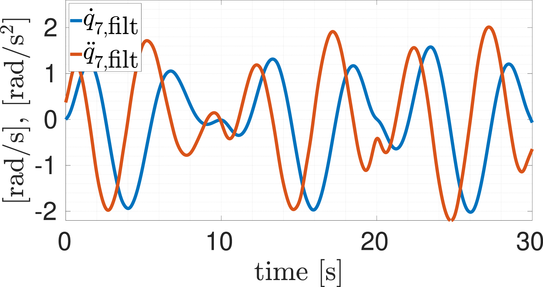
This section fully evaluates estimator equation (6), with seven IMUs installed on all robot links. For the sake of simplicity, the estimator is tuned blindly and equally, independently of each IMU SNR. Five (on links 1, 2, 3, 5, 7) out of seven IMUs in this setup are used for estimating robot link velocity and acceleration via a state-of-the-art method (Fennel et al., 2022) called full Kalman filter (KFF). In this method, error in the measurement is compensated by considering additive parameters in the measurement function. This error is sourced from inaccuracies in the sensor position and the additive sensor bias. However, we do not account for sensor position errors in this section. Furthermore, the number of employed IMUs is independent of the robot’s degrees of freedom. Therefore, any arbitrary number of IMUs can be used. The robot moves along the excitation trajectory explained in Section Full Link Variable Estimation. The ground truth ( $\dot{\mathit{q}}$ and $\ddot{\mathit{q}}$ ) is based on numerical differentiation of the measured link positions q _m. In order to minimize the errors in the ground truth, the signal is (lag-free) filtered. Since the link variables are estimated recursively from the first to the seventh link, the seventh link is most prone to accumulative errors. Therefore, for the sake of clarity, we mainly report the last link estimation results in Figures 21–23(a) and (b). Figure 21 shows the seventh link reference trajectories. Although effective for simpler robots with fewer DoFs (Fennel et al., 2022), Figure 22 shows the divergence of KFF when estimating link velocity and acceleration for our 7 DoF manipulator. The reason may be that the steady-state Kalman gain is dependent on the parameters ⁶ in this approach. In fact, in joint state and parameters estimations, it is evident that the filter stability and, consequently, convergence may be poor when the Kalman gain is a function of the parameters (Ljung, 1979). Furthermore, Figures 23(a) and (b) depict the last link velocity and acceleration error signals, respectively. The error signals in these figures are obtained via

$\begin{array}{ll}\hfill {\widehat{\dot{\mathit{e}}}}_{\text{q}}& ={\dot{\mathit{q}}}_{\text{filt}}-\widehat{\dot{\mathit{q}}},\hfill \\ \hfill {\widehat{\ddot{\mathit{e}}}}_{\text{q}}& ={\ddot{\mathit{q}}}_{\text{filt}}-\widehat{\ddot{\mathit{q}}},\hfill \\ \hfill \mathrm{\Delta }{\mathit{e}}_{\text{q}}& ={\dot{\mathit{q}}}_{\text{filt}}-\frac{\mathrm{\Delta }{\mathit{q}}_{\text{m}}}{\mathrm{\Delta }t},\hfill \\ \hfill {\mathrm{\Delta }}^2{\mathit{e}}_{\text{q}}& ={\ddot{\mathit{q}}}_{\text{filt}}-\frac{{\mathrm{\Delta }}^2{\mathit{q}}_{\text{m}}}{\mathrm{\Delta }{t}^2},\hfill \end{array}$

(59)

with Δ q _m/Δt and Δ² q _m/Δt² being the numerical and second-order numerical differentiation of the measured link position q _m, respectively. These signals are filtered with a second-order low-pass filter with a 20 Hz cutoff frequency.

Figure 21.

Seventh link velocity and acceleration reference trajectories in the full DoF experiment. In this experiment, each robot link is equipped with one IMU. The robot moves along an excitation trajectory and all kinematic states are estimated using estimator equation (6). Here, “filt” refers to the encoder signal, which is differentiated and filtered via a lag-free filtering method.

Figure 22.

Seventh link velocity and acceleration estimation using the state-of-the-art method. KFF denotes the full Kalman filter in this figure.

Figure 23.

The experiment for evaluating estimator equation (6) introduced in Section Link Velocity and Acceleration Estimation. (a) The velocity error signal generated by different methods for the seventh link. (b) The acceleration error signal generated by different methods for the seventh link. (c) RMSE of the estimated/computed link velocity via different methods for all links. (d) RMSE of the estimated/computed link acceleration via different methods for all links. (e) RMSE of the estimated/computed seventh link velocity via different methods, when other links are at rest. (f) RMSE of the estimated/computed seventh link acceleration via different methods, when other links are at rest.

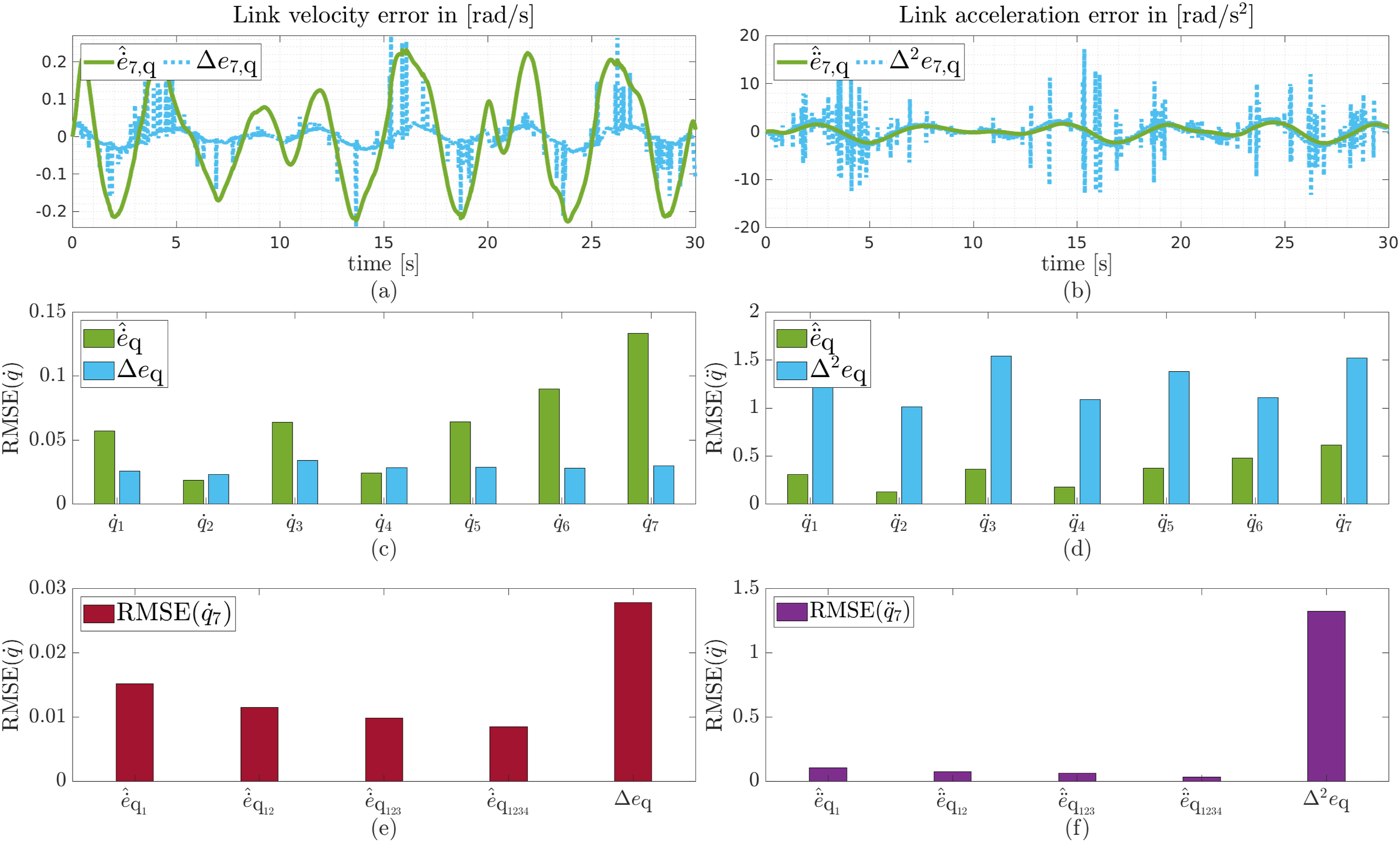
According to Figure 23(c), where the RMSE $(\dot{\mathit{q}})$ for all links is depicted, the numerical differentiation outperforms (with RMSE $<0.03$ rad/s) the proposed method (with RMSE up to 0.13 rad/s for the last link). Moreover, the SNR issue is apparent in the links where the distance from the rotation axis cannot be optimized. Furthermore, the accumulative error contributes to further estimation deviations in the last links. The proposed estimator equation (6), however, outperforms second-order numerical differentiation. The main reason is that the quantization error is amplified after each differentiation, such that the acceleration signal loses reliability (see Figure 23(d)). On the other hand, the SNR issue and cumulative error are apparent in the estimated link acceleration via estimator equation (6), as well.

In the last part of the experiments, we fuse up to four IMUs to estimate the last link velocity and acceleration while the other links are at rest (see Figures 23(e) and (f)). In these figures, ${\widehat{\dot{e}}}_{q_1}$ and ${\widehat{\ddot{e}}}_{q_1}$ represent the RMSE of the link velocity and acceleration estimation, respectively, when only one IMU is used. Moreover, ${\widehat{\dot{e}}}_{q_{12}}$ and ${\widehat{\ddot{e}}}_{q_{12}}$ are estimation errors when IMUs are fused via

$\begin{array}{ll}\hfill {}^{S_1}\mathit{a}_{12}& =\frac{1}{2}{}^{S_1}\mathit{a}_{S_1}+\frac{1}{2}{}^{S_1}\mathit{a}_{S_{1\leftarrow 2}},\hfill \\ \hfill {\mathit{\omega }}_{12}& =\frac{1}{2}{\mathit{\omega }}_{S_1}+\frac{1}{2}{\mathit{\omega }}_{S_2},\hfill \end{array}$

(60)

with ${}^{S_1}\mathit{a}_{12}$ being the fused acceleration at the S₁ frame. Moreover, ${}^{S_1}\mathit{a}_{S_1}$ and ${}^{S_1}\mathit{a}_{S_{1\leftarrow 2}}$ denote the acceleration measured by S₁ and S₂ at sensor S₁ frame ⁷ , respectively. Here, ${}^{S_1}\mathit{a}_{S_{1\leftarrow 2}}$ is computed similarly to equation (56). Furthermore, ω ₁₂ is the fused angular velocity, which consists of angular velocity measured by S₁ $({\mathit{\omega }}_{S_1})$ and S₂ $({\mathit{\omega }}_{S_2})$ . Fusion with equal weighting (similar to equation (60)) is also used when we fuse three and four IMUs. The corresponding estimation errors are denoted by ${\widehat{\dot{e}}}_{q_{123}}$ and ${\widehat{\dot{e}}}_{q_{1234}}$ for link velocity and ${\widehat{\ddot{e}}}_{q_{123}}$ and ${\widehat{\ddot{e}}}_{q_{1234}}$ for acceleration, respectively. Since only the seventh link is actuated in this experiment, the accumulative error is absent in the estimations. Therefore, ${\widehat{\dot{e}}}_{q_1}$ and ${\widehat{\ddot{e}}}_{q_1}$ are already lower than Δe _q and Δ²e _q , respectively. Moreover, with more sensors fused, the estimation error decreases.

Conclusion

Fully accurate state estimation in robot manipulators as a whole has been an unsolved problem. The lack of accurate simultaneous link-side position, velocity and acceleration at high accuracy and bandwidth had to be circumvented with various practical approaches. However, in both rigid robot systems and flexible-joint robots, link acceleration has not been an available signal for control yet.

In this work, we introduced a novel nonlinear estimator framework for acquiring accurate, high-bandwidth link-side velocity and acceleration in flexible-joint robots based on fusing redundant link IMUs with standard proprioceptive measurements, namely, motor position (and joint torque for flexible joint systems). Specifically, we provide the mathematical framework and a computational design approach to optimal IMU placement for subsequent use in estimation and control. Based on the development and analysis of centralized and decentralized fusion architectures for redundant IMUs for link state estimation, the capability of the latter to detect faulty sensors is exploited. A novel fault detection and isolation mechanism is devised that is able to detect arbitrary sensor failures in the considered class of robot systems. The extensive design examples, simulations and experiments validate the novel robust state estimation and fault handling framework as well as underline its practical relevance.

Finally, the link velocity and acceleration observer is extensively evaluated by installing one IMU per manipulator link for the state-of-the-art manipulator Franka Emika Robot. As used in standard industrial practice, numerical differentiation of robot link position is a valid method for obtaining link velocity. However, our method clearly outperforms second-order numerical differentiation when it comes to link acceleration estimation. We also showed that fusing more than one IMU for each link further improves the estimation accuracy. Current limitations of our experimental analysis are the external mounting and external synchronization, which introduce significant disturbances such as mounting compliance, higher delays and thus larger estimation errors. It is therefore reasonable to assume that with tight mechatronic integration and future even more capable IMU technology, our approach will be able to safely and robustly estimate both link velocity and acceleration under a unified framework.

Looking ahead, several developments are expected to unlock an additional tier of performance. Integrating the IMUs directly into the mechatronic structure—rather than attaching them externally—will suppress mounting compliance and vibration. Running the fusion algorithms on modern joint-level hardware at sampling rates of 5 kHz or higher with latencies well below 2 ms will widen usable bandwidth (10 Hz for robot manipulators) and shrink estimation delay. At this bandwidth, the IMU signal-to-noise ratios have already improved by about 60% over the past two decades (from roughly 45 dB to nearly 70 dB), and each further increment is poised to translate directly into observer accuracy. In parallel, recent advances in high-resolution joint-torque sensing promise complementary gains when those signals are incorporated into the framework.

With such tight mechatronic integration and the continued evolution of IMU and torque-sensor technology, our approach is positioned to deliver safe, robust and high-bandwidth estimation of both link velocity and link acceleration under a unified framework for next-generation manipulators.