
Abstract
This article presents MAPS2: a distributed algorithm that allows multi-robot systems to deliver coupled tasks expressed as Signal Temporal Logic (STL) constraints. Classical control theoretical tools addressing STL constraints either adopt a limited fragment of the STL formula or require approximations of min/max operators. Meanwhile, works maximising robustness through optimisation-based methods often suffer from local minima, thus relaxing any completeness arguments due to the NP-hard nature of the problem. Endowed with probabilistic guarantees, MAPS2 provides an autonomous algorithm that iteratively improves the robots’ trajectories. The algorithm selectively imposes spatial constraints by taking advantage of the temporal properties of the STL. The algorithm is distributed in the sense that each robot calculates its trajectory by communicating only with its immediate neighbours as defined via a communication graph. We illustrate the efficiency of MAPS2 by conducting extensive simulation and experimental studies, verifying the generation of STL satisfying trajectories.
Keywords
Introduction
Autonomous robots can solve significant problems when provided with a set of guidelines. These guidelines can be derived from either the physical constraints of the robot, such as joint limits, or imposed as human-specified requirements, such as pick-and-place objects. An efficient method of imposing such guidelines is by using logic-based tools, which enable reasoning about the desired behaviour of robots. These tools help us describe the behaviour of a robot at various levels of abstraction, such as interactions between its internal components to the overall high-level behaviour of the robot (Lamport, 1983). This strong expressivity helps us efficiently encode complex mission specifications into a logical formula. Recent research has focused on utilising these logic-based tools to express requirements on the behaviour of robots. Once these requirements are established, algorithms are developed to generate satisfying trajectories. Such is the focus of our work.
Examples of logic-based tools include formal languages, such as Linear Temporal Logic (LTL), Metric Interval Temporal Logic (MITL), and Signal Temporal Logic (STL). The main distinguishing feature between these logics is their ability to encode time. While LTL operates in discrete-time and discrete-space domain, MITL operates in the continuous-time domain but only enforces qualitative space constraints. On the other hand, STL allows for the expression of both qualitative and quantitative semantics of the system in both continuous-time and continuous-space domains (Maler and Nickovic, 2004). STL thus provides a natural and compact way to reason about a robot’s motion since it operates in a continuously evolving space-time environment. Additionally, STL is accompanied by a robustness metric which allows us to determine the extent of satisfaction compared to only absolute satisfaction (Donzé, 2013).
Another important property of autonomous robots is their ability to coordinate and work in teams. The use of multiple robots is often necessary in situations where a single robot is either insufficient, the task is high-energy demanding, or unable to physically perform certain tasks. However, multi-robot systems present their own set of challenges, such as communication overload, the need for a central authority for commands, and high computational demands. The challenge, therefore, is to derive solutions for multi-robot problems utilising logic-based tools, ensuring the achievement of specified high-level behaviour.
In this article, we propose • The algorithm’s effectiveness lies in its ability to distribute STL planning for multiple robots and in providing a mechanism to decouple the STL formula among robots, thereby facilitating the distribution of tasks. • As opposed to previous work, it covers the entire STL formula and is not limited to a smaller fragment. It reduces conservatism by eliminating the need for approximations of max/min operators and samples in continuous time to avoid abstractions. • It incorporates a wide range of coupled constraints (both linear and nonlinear) into the distributed optimisation framework, enabling the handling of diverse tasks such as pick-and-place operations and time-varying activities like trajectory tracking. • We present extensive simulation and hardware experiments that demonstrate the execution of complex tasks using MAPS2.
Additionally, the algorithm presented is sound, meaning that it produces a trajectory that meets the STL formula and is probabilistically complete, meaning that it will find such a trajectory if one exists.
In our prior study (Sewlia et al., 2023), we addressed the STL motion-planning problem for two coupled agents. There, we extended the conventional Rapidly exploring Random Trees (RRT) algorithm to sample in both the time and space domains. Our approach incrementally built spatio-temporal trees through which we enforced space and time constraints as specified by the STL formula. The algorithm employed a sequential planning method, wherein each agent communicated and waited for the other agent to build its tree. In contrast, the present work addresses the STL motion-planning problem for multiple robots. Here, our algorithm adopts a distributed optimisation-based approach, where spatial and temporal aspects are decoupled to satisfy the STL formula. Instead of constructing an incremental tree, as done in the previous work, we introduce a novel metric called the validity domain and initialise the process with an initial trajectory. In the current research, we only incorporate the STL parse tree and the Satisfaction variable tree from our previous work. Additionally, we present experimental validation results and introduce a novel STL verification architecture.
The rest of the paper is organised as follows. The related work is presented next. Then preliminaries and problem formulation are discussed, followed by the decomposition of the STL formula into temporal and spatial constraints. Next, the main algorithm MAPS2 with its analyses is presented. Afterwards, simulations of various robotics tasks are shown, followed by experimental validation on a real multi-robot setup. Finally, the conclusion is presented.
Related work
In the domain of single-agent motion planning, different algorithms have been proposed to generate safe paths for robots. Sampling-based algorithms, such as CBF-RRT (Yang et al., 2019), have achieved success in providing a solution to the motion-planning problem in dynamic environments. However, they do not consider high-level complex mission specifications. Works that impose high-level specifications in the form of LTL, such as Ayala et al. (2013); Bhatia et al. (2010); Fainekos et al. (2009); Vasile and Belta (2013), resort to a hybrid hierarchical control regime resulting in abstraction and explosion of state-space. While a mixed-integer program can encode this problem for linear systems and linear predicates (Wolff et al., 2014), the resulting algorithm has exponential complexity, making it impractical for high-dimensional systems, complex specifications, and long duration tasks. To address this issue, Kurtz and Lin (2022) propose a more efficient encoding for STL to reduce the exponential complexity in binary variables. Additionally, Lindemann and Dimarogonas (2017) introduce a new metric, discrete average space robustness, and composes a Model Predictive Control (MPC) cost function for a subset of STL formulas.
In multi-agent temporal logic control, works such as Verginis and Dimarogonas (2018) and Kress-Gazit et al. (2009) employ workspace discretisation and abstraction techniques, which we avoid in this article due to it being computationally demanding. Some approaches to STL synthesis involve using mixed-integer linear programming (MILP) to encode constraints, as previously explored in Belta and Sadraddini (2019), Raman et al. (2014), and Sadraddini and Belta (2015). However, MILPs are computationally intractable when dealing with complex specifications or long-term plans because of the large number of binary variables required in the encoding process. The work in Sun et al. (2022) encodes a new specification called multi-agent STL (MA-STL) using mixed-integer linear programs (MILP). However, the predicates here depend only on the states of a single agent, can only represent polytope regions, and finally, temporal operations can only be applied to a single agent at a time. In contrast, this work explores coupled constraints between robots and predicates are allowed to be of nonlinear nature.
As a result, researchers have turned to transient control-based approaches such as gradient-based, neural network-based, and control barrier-based methods to provide algorithms to tackle the multi-robot STL satisfaction problem (Kurtz and Lin, 2022). Such approaches, at the cost of imposing dynamical constraints on the optimisation problem, often resort to using smooth approximations of temporal operators at the expense of completeness arguments or end-up considering only a smaller fragment of the syntax (Lindemann et al., 2017; Charitidou and Dimarogonas, 2021; Chen and Dimarogonas, 2022; Lindemann and Dimarogonas, 2018). STL’s robust semantics are used to construct cost functions to convert a synthesis problem to an optimisation problem that benefits from gradient-based solutions. However, such approaches result in non-smooth and non-convex problems and solutions are prone to local minima (Gilpin et al., 2020). In this work, we avoid approximations and consider the full expression of the STL syntax. The proposed solution adopts a purely geometrical approach to the multi-robot STL planning problem. Our current focus is directed towards the planning problem, specifically the generation of trajectories that fulfil STL constraints, rather than the dynamical constraints or the precise control techniques used to execute the trajectory.
Preliminaries and problem formulation
In this section, we start by introducing STL and STL parse tree, followed by the problem formulation.
Signal Temporal Logic (STL)
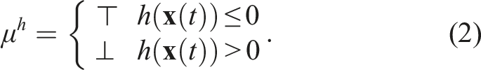
Let

(Madsen et al., 2018). The time horizon th(φ) of an STL formula φ is recursively defined as
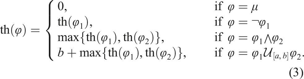
In this work, we consider only time bounded temporal operators, that is, when th(φ) < ∞. In the case of unbounded STL formulas, it is only possible to either falsify an always operator or satisfy an eventually operator in finite time, thus we consider only bounded time operators. Next, we state a common assumption regarding the STL formula.
The STL formula is in positive normal form, that is, it does not contain the negation operator.
The above assumption does not cause any loss of expression of the STL syntax (1). As shown in Sadraddini and Belta (2015), any STL formula can be written in positive normal form by moving the negation operator to the predicate.
STL parse Tree
An STL parse tree is a tree representation of an STL formula (Sewlia et al., 2023). It can be constructed as follows: • Each node is either a temporal operator node • temporal and logical operator nodes are called set nodes; • a root node has no parent node and a leaf node has no child node. The leaf nodes constitute the predicate nodes of the tree.
A path in a tree is a sequence of nodes that starts at a root node and ends at a leaf node. The set of all such paths constitutes the entire tree. A subpath is a path that starts at a set node and ends at a leaf node; a subpath could also be a path. The resulting formula from a subpath is called a subformula of the original formula. In the following, we denote any subformula of an STL formula φ by
The STL parse tree and the satisfaction variable tree for the STL formula

Problem formulation
We consider a team of
For an STL formula φ = (‖x1 − x2‖ > 5) ∧ (‖x2 − x3‖ < 2), h(1) = 5 − ‖x1 − x2‖ and h(2) = ‖x2 − x3‖ − 2. Then
Let K
c
≤ K denote the number of coupled predicate functions, and let these be indexed as
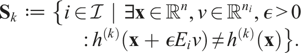
Next, let L
i
be the number of independent predicate functions that involve only the states of robot i, with
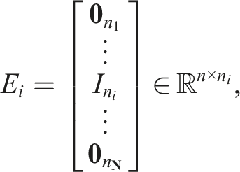
Let

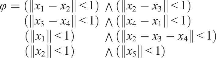
Consider the STL formula, Now we are ready to define the communication structure of the multi-robot system, which is dictated by a graph. Let the communication graph be given by
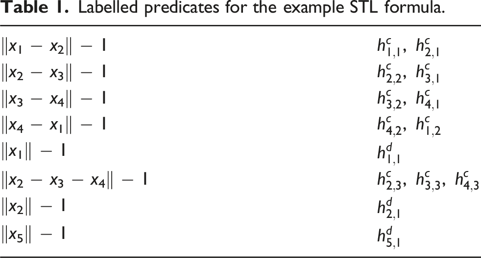
Labelled predicates for the example STL formula.
If (i, j) ∈
We further assume that, every coupled predicate function induces an edge, ensuring that all state variables needed to compute the predicate function are locally available for each robot.
If there exists k ∈ {1, …, K} such that i, j ∈
Note that the aforementioned assumption implies that the graph is undirected, that is, (i, j) ∈
An algorithm is called distributed, if it can be executed individually by each robot i (a local version of the algorithm) by using only information from its neighbours
This definition of distributed algorithm does not allow for any global information sharing among robots that are not neighbours with each other, thus a central computer cannot evaluate an STL formula. For example, consider the STL formula:
We are now ready to formally state the problem addressed in this paper.
It should be noted that we do not currently address the closed-loop stability of the underlying multi-robot system. Instead, we focus on the trajectory generation aspect and rely on existing low-level control approaches to track the generated trajectories. For more information, see Remark 3. The above problem is addressed assuming that at least one such solution exists. This will help us provide probabilistic completeness guarantees later on. Formally, we state the following assumption:
There exists at least one
STL formula decomposition
In this section, we present how to retrieve spatial and temporal constraints from a given STL formula φ.
Spatial constraints
In Section ‘Problem Formulation', we provisioned each predicate function h(k)(
For robot i, cast the constraints (6) into the cost function F
i
as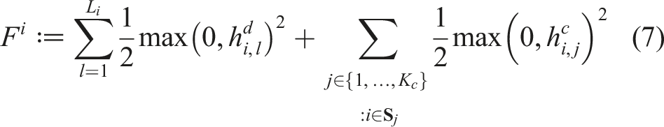
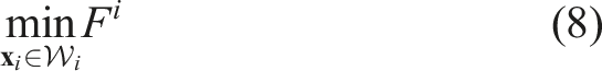
The solution for finding the global minimum of a non-convex function is a subject of extensive research. We argue that employing gradient descent with random initialisations is adequate for addressing this problem, particularly since the initialisations are sampled from a compact set,
algorithm as described in Algorithm 9.3 of Boyd and Vandenberghe (2004), utilising initial conditions
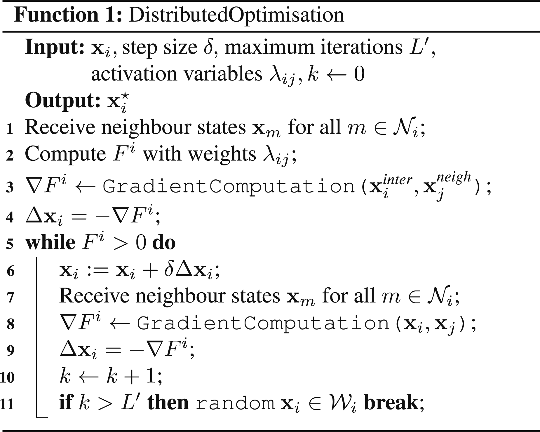
The robots solve their respective optimisation problem cooperatively in a distributed manner via inter-neighbour communication. This makes the problem distributed, as every interaction between robots is part of the communication graph. Given the nature of the optimisation problem, there is a trade-off between robustness and optimisation performance since
Consider a system with 3 agents and the corresponding states {x1, x2, x3}, and let the STL formula be: φ = (‖x1 − x2‖ > 5) ∧ (‖x2 − x3‖ < 2); then, the functions F
i
, for i ∈ {1, 2, 3}, are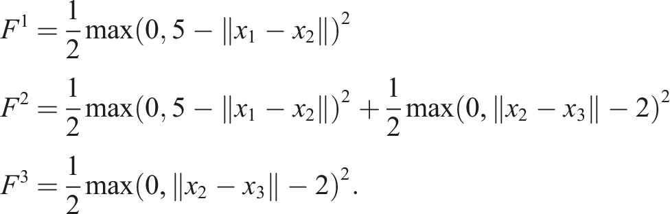
Now that spatial constraints are encoded into the optimisation problem, we are ready to encode temporal constraints in the following section, thus completing our STL decomposition into spatial and temporal constraints.
Temporal constraints
We now introduce the concept of validity domain, a time interval associated with every predicate and defined for every path in the STL formula. This interval represents the time domain over which each predicate applies and is defined as follows:
The validity domain 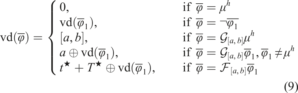
The above definition of t⋆ is necessary due to the redundancy of the eventually operator; we must ascertain the specific instances where the eventually condition is met to ensure finding a feasible trajectory. Additionally, we need to maintain the history of T⋆ for nested temporal operators which require recursive satisfaction. The validity domain is determined for each path of an STL formula in a hierarchical manner, beginning at the root of the tree, and each path has a distinct validity domain. The number of leaf nodes in an STL formula is equal to the total number of validity domains. In Definition 3, we do not include the operators ∧ and ∨ because they do not impose temporal constraints on the predicates and thus inherit the validity domains of their parent node. If there is no parent node, operators ∧ and ∨ inherit the validity domains of their child node.
The validity domain is specially defined in the following cases. If a path contains only predicates, the validity domain of μ
h
is equal to the time horizon of φ (i.e. vd(μ
h
) = th(φ)). Furthermore, if a path contains nested formulas with the same operators, such as
Consider the following examples of the validity domain: • • • • • Regarding the STL formula in equation (4), the validity domains are defined for the following paths:
We use the following notational convenience in this work: if a parent node of a leaf node of a path
Suppose
The proof follows from the construction of the optimisation function (7) and the validity domain. Notice that if the optimisation problem (8) converges to the desired minima at F
i
( In the next Section, we present how to integrate the validity domain with the optimisation problem in (8), completing thus the spatial and temporal integration.
Main results
In this section, we present the algorithm for generating continuous trajectories that meet the requirements of a given STL formula φ. The algorithm is executed by the robots offline in a distributed manner, in the sense that they only communicate with their neighbouring robots. The algorithm builds a tree
In what follows, we give a high-level description of the algorithm. The general idea is to start with an initial trajectory that spans the time horizon of the formula th(φ), then repeatedly sample random points along the trajectory and use gradient-based techniques to find solutions that satisfy the specification at these points. More specifically, the algorithm begins by connecting the initial and final points
Before we get into the technical details, let us consider an example of 4 agents, represented by the colours blue, green, yellow and magenta, to illustrate the procedure. Suppose, at a specific instance in time, say t0, the STL formula requires agent 1 (
We begin the process by connecting the initial and final points  ) and agent 2 (
 ) to be more than 6 units apart and agent 3 (
 ) and agent 4 (
 ) to be closer than 6 units, that is, for ϵ > 0,
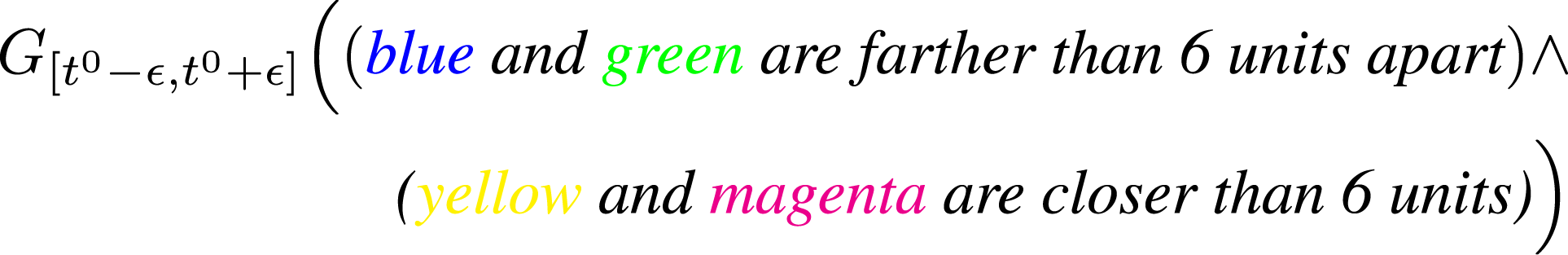
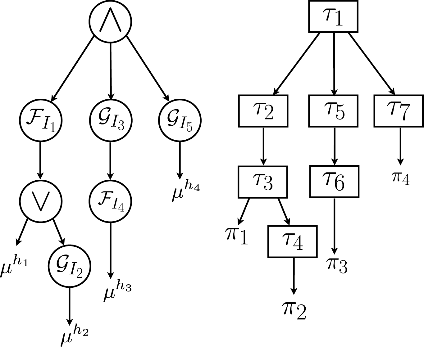
STL parse tree and satisfaction variable tree for the formula in (4).
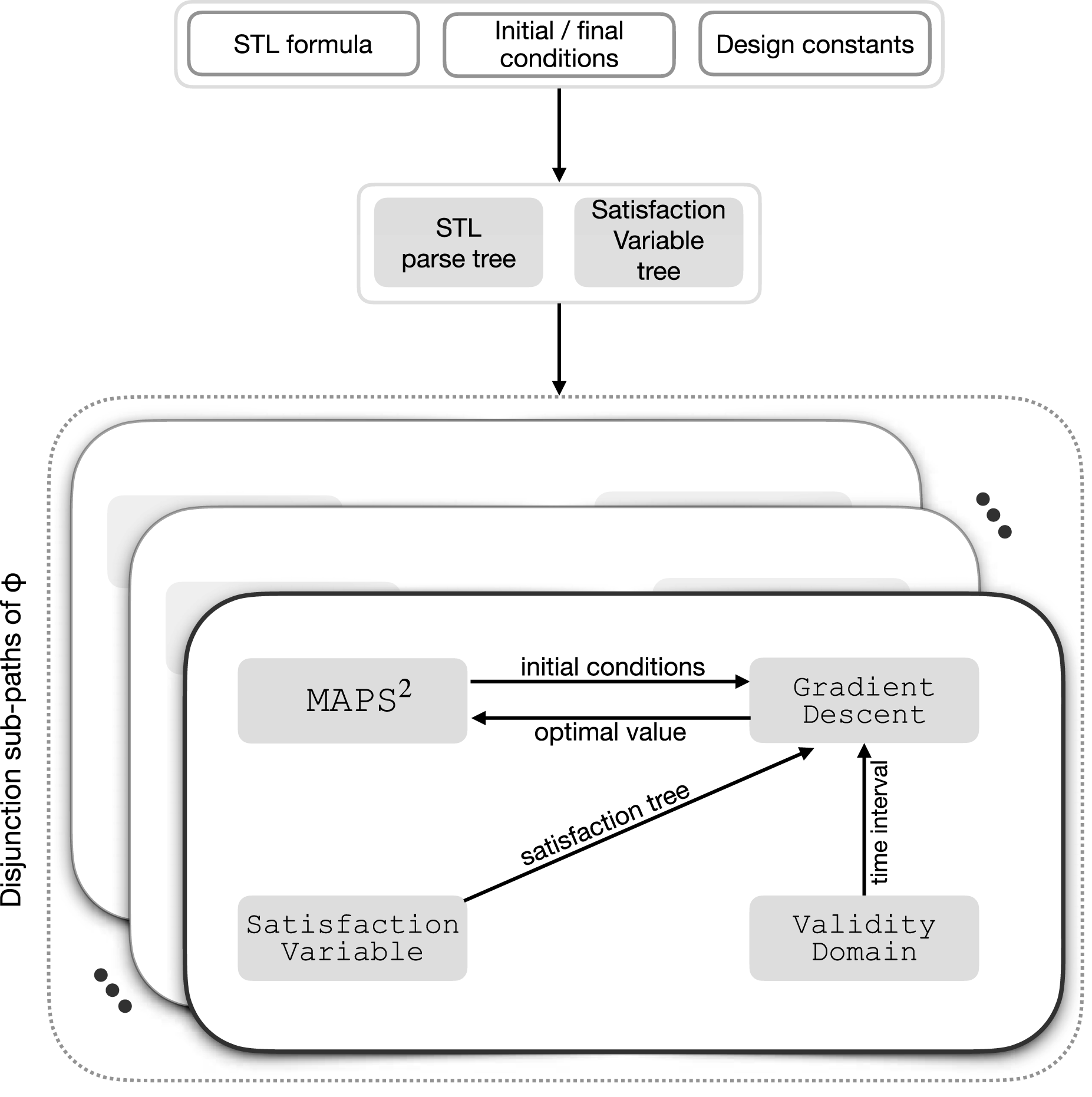
MAPS2
The architecture of the algorithm Illustration of the proposed algorithm.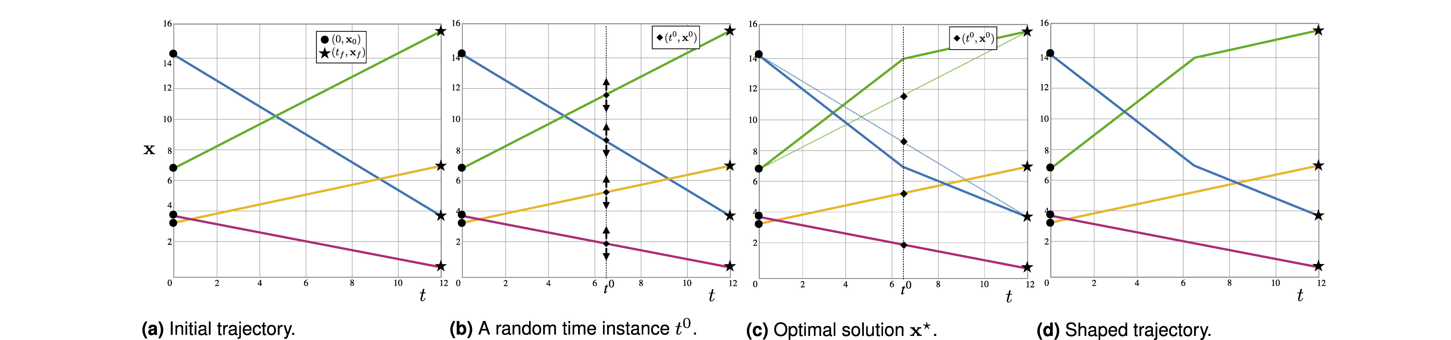
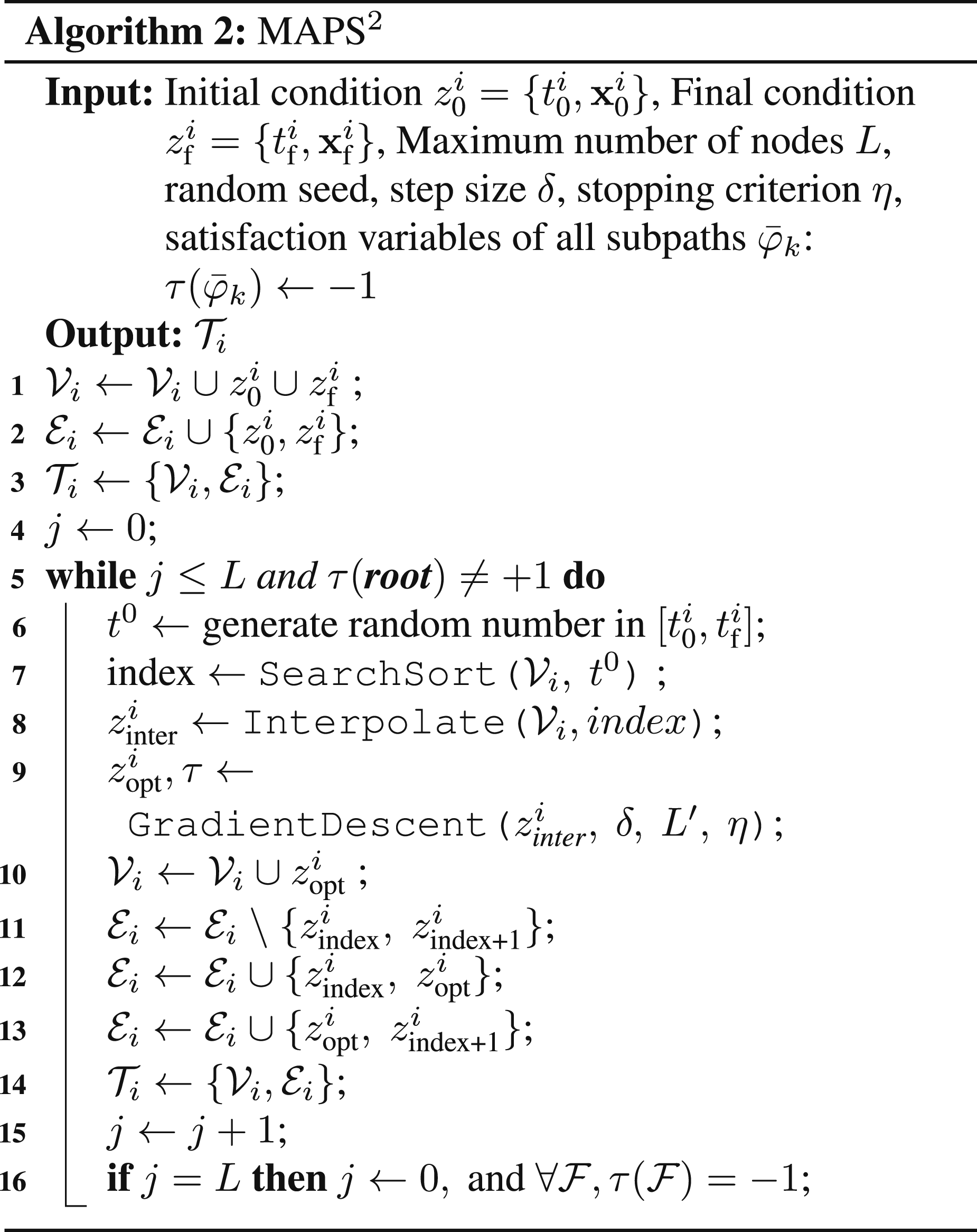
These steps are implemented as follows: In line 4, the 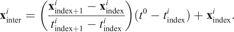
Moreover, as a safeguard, if a solution remains undiscovered following L iterations, line 4 initiates a reset procedure. This involves setting the satisfaction variable for all eventually operators back to −1 and restarting the search. Since we assume that at least one viable solution always exists (refer to Assumption 4), the absence of a solution occurs solely when an eventually operator is satisfied at an impractical instance of time. Such an impractical instance of time affects the solution of the algorithm since there are redundancies in picking the satisfaction instance (
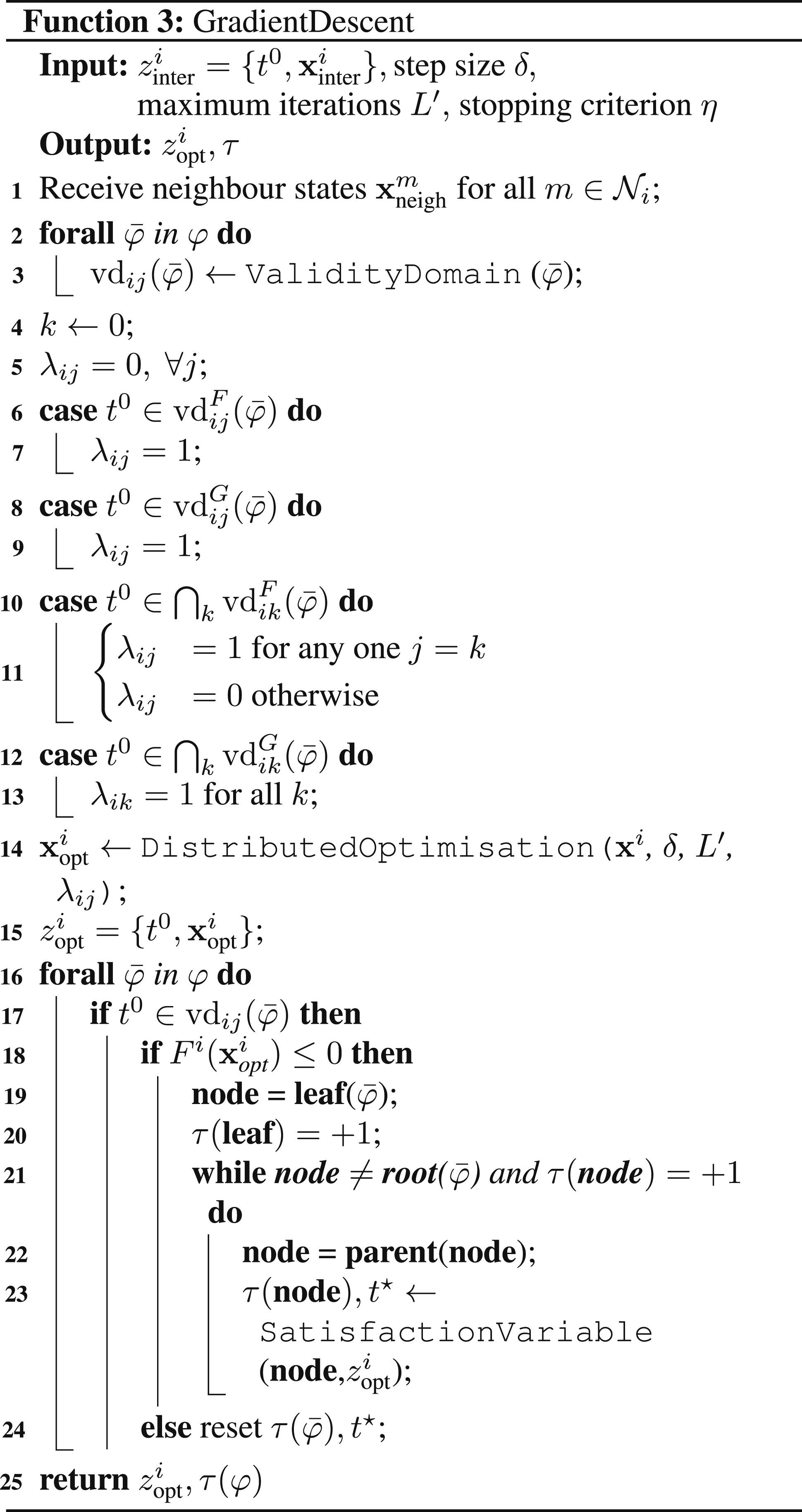
GradientDescent
The function is presented in Function 3 and computes the optimal value,
Based on the validity domain, the Function 3 determines which predicate functions are active in (7) at every sampled time instance t0. The Function • If • If
The indices i and j in λ
ij
and vd
ij
refer to robot i and the jth predicate function associated with robot i, respectively. Here j ∈ {1, …, K
i
}. We distinguish three cases: if the sampled point belongs to the validity domain of a single eventually operator and/or a single always operator, λ
ij
= 1. If the sampled point belongs to the validity domain of multiple eventually operators, we activate only one of them at random, that is, λ
ij
= 1 only for one of them. This avoids enforcing conflicting predicates as it can happen that multiple eventually operators may not be satisfied at the same time instance (e.g.
In lines 21-34, the algorithm updates the satisfaction variable of all paths in the STL formula that impose restrictions on robot i’s states. The algorithm goes bottom-up, starting from the
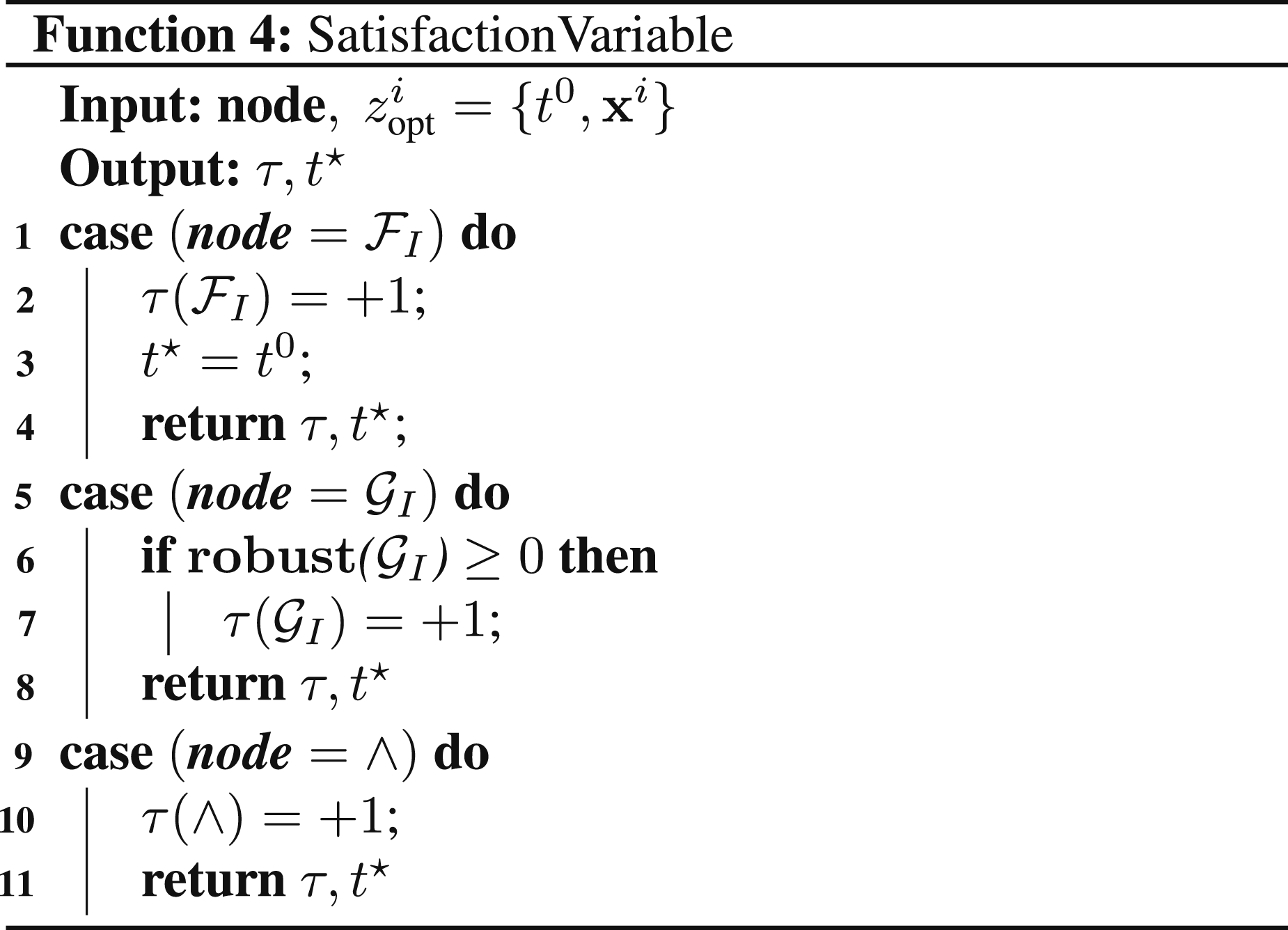
SatisfactionVariable
This function, presented in Function 4, updates the satisfaction variable tree, τ. The aforementioned procedure decides if the satisfaction variable corresponding to each node listed is +1 (satisfied) or −1 (not yet satisfied). The discussion of handling disjunction operators is deferred to Section ‘MAPS2:Branch-and-Pick for Disjunctions', as they are handled differently. Considering the premise that the predicate is true, as indicated in line 27 of Function 3, we evaluate the satisfaction variable as follows: • • • ∧: This set node returns the satisfaction variable as +1 since it does not impose spatial or temporal restrictions.
Branch-and-pick for disjunctions
In our approach, we address disjunctions as follows: Given an STL formula of the form φ =∨i∈1,…,Kϕ
i
, which can also be represented as φ = ∨(ϕ1, ϕ2, …, ϕ
K
), we divide it into K individual STL formulas. The agents then run Algorithm 2 separately for each φ = ϕ
i
, where i ∈ 1, …, K. For instance, consider the STL formula represented as (4) Architecture of the proposed algorithm.

Analysis
In this section, we analyse the proposed algorithm and arrive at proving the probabilistic completeness.
Let the set
Starting with an initial linear trajectory in the augmented time-space domain, each uniformly sampled time point t0 corresponds to a position
Next, divide the trajectory Disjunction representation for disjunctive components using STL parse tree.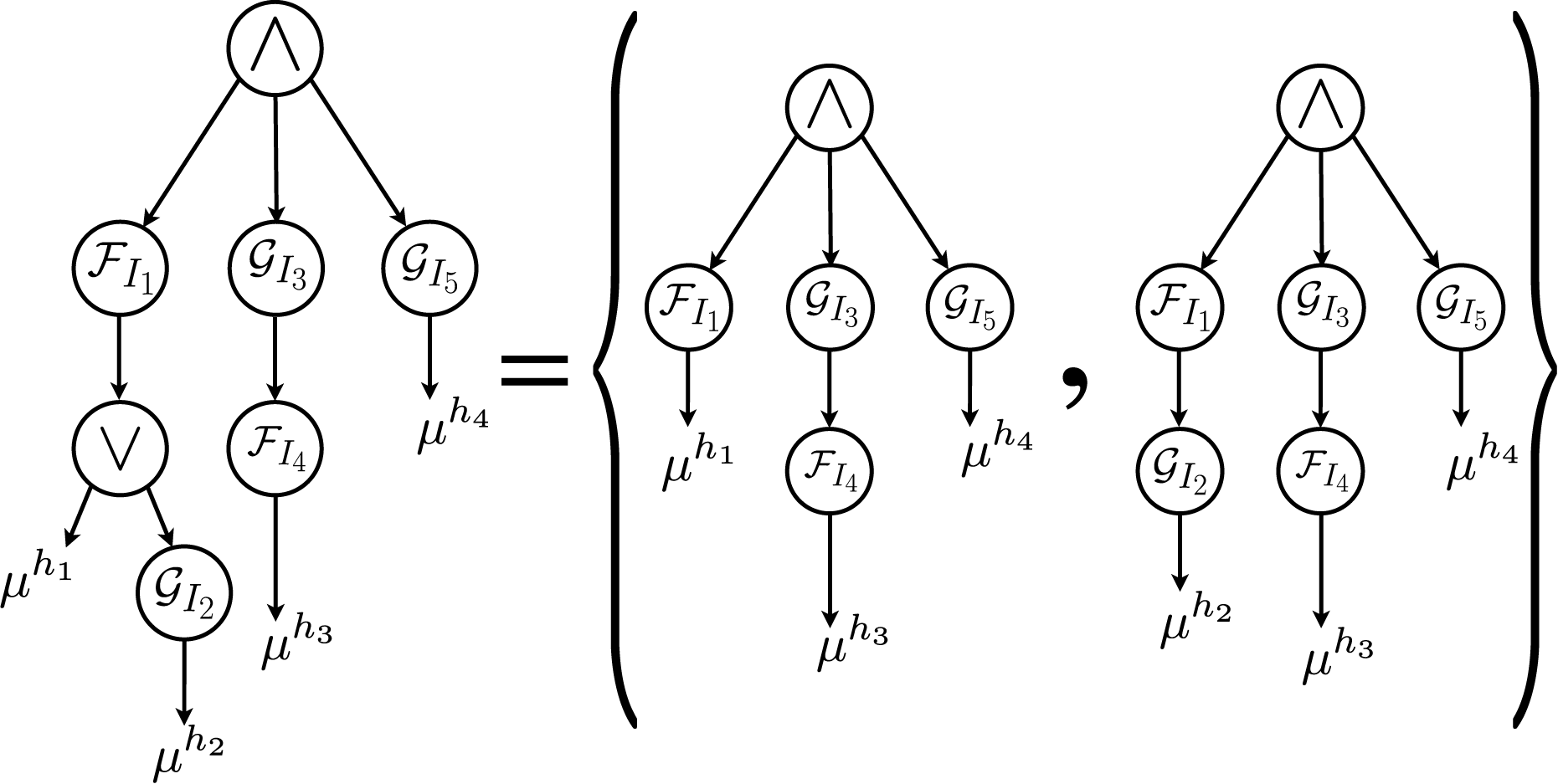
Let a constant L and probability p such that
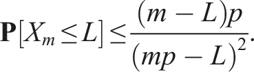
The probability of not having L successful trials after m samples can be expressed as Next, we present a final lemma which helps us prove the probabilistic completeness of the algorithm.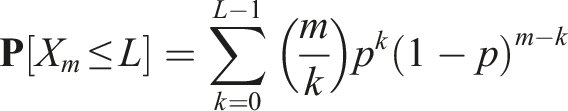
No sampled point
The algorithm initiates by setting all satisfaction variables, τ, to −1, as inputs to Algorithm 2. These variables are updated in Function 4 designed for evaluating whether τ meets the satisfaction criteria. The function adjusts τ in accordance with the definition of STL operators presented in the preliminaries section, ensuring that updates accurately reflect the satisfaction status. Furthermore, the update to τ( Next, the paper’s final result is presented, which states that the probability of the algorithm providing an STL formula satisfying trajectory (if one exists) approaches one as the number of samples tends to infinity. This is a desirable property for sampling-based planners and such algorithms are termed probabilistically complete.
Algorithm 2 is probabilistically complete.
The proof follows from Lemmas 1, 2, and 3. From Lemma 1 and Lemma 3, we know that every sample added to the trajectory satisfies the STL formula. Thus, what needs to be shown is that the algorithm samples infinitely many times and covers the entire time horizon. From Lemma 2, we know that the probability of covering the entire time horizon is 1 −
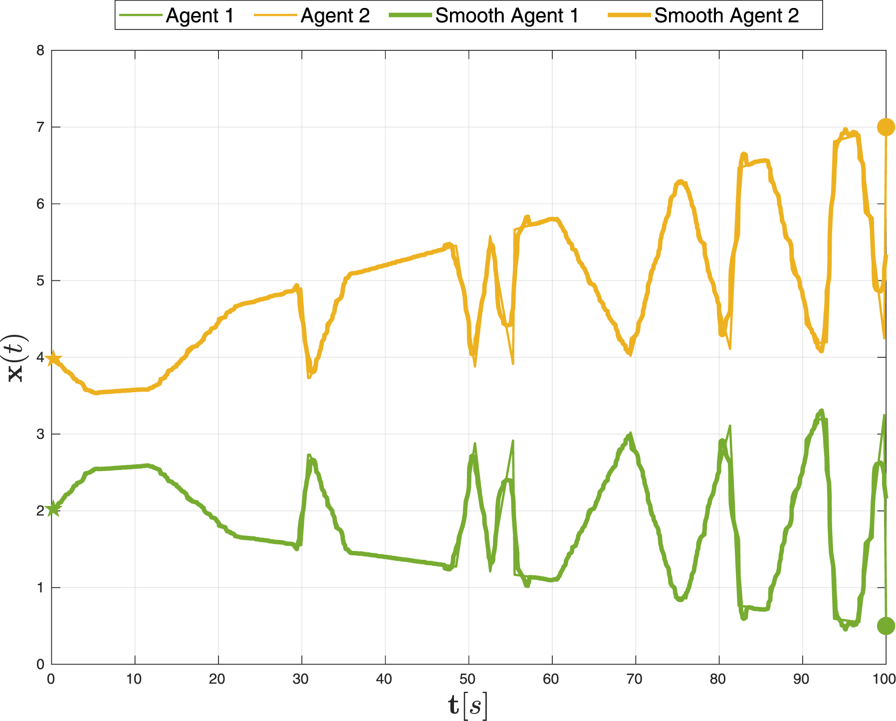
Our algorithm can be endowed in a post-processing stage with a module that smoothens the trajectory to avoid large accelerations. However, care needs to be taken since the smoothened paths may no longer satisfy the STL formula. One could also use more sophisticated approaches like B-splines to impose velocity and acceleration limits as shown in Lapandić et al. (2024).
At present, our approach does not incorporate kinematic or dynamic constraints. Incorporation of such constraints could be attempted by either deploying the kinodynamic version of the RRT algorithm (Webb and van Den Berg, 2012), or by using an existing low-level controller to track the generated open-loop trajectories. Some examples of such controllers include the Model Predictive Controller (Poignet and Gautier, 2000) and the input constrained Prescribed Performance Controller (Fotiadis and Rovithakis, 2024; Trakas and Bechlioulis, 2023). This incorporation is by no means straightforward but requires fusion with another type of methodological machinery that goes beyond the scope of the current work. Moreover, such controllers have been developed for a large variety of dynamical systems and hence the proposed algorithm is practical and applicable to a large class of robots.
Simulations
In this section, we present simulations of various scenarios encountered in a multi-robot system. Restrictions are imposed using an STL formula and MAPS2 is utilised to create trajectories that comply with the STL formula. In the following we consider 4 agents, with δ = 0.1, η = 0.01 and L = L′ = 100. The simulations were run on an 8 core Intel® CoreTM i7 1.9 GHz CPU with 16 GB RAM. 2
Collision avoidance
We begin with a fundamental requirement in multi-robot systems: avoiding collisions. In this scenario, it is assumed that all agents can communicate or sense each other’s positions. The following STL formula is used to ensure collision avoidance in the interval 20[s] to 80[s]: Illustration of 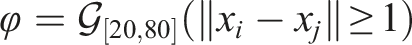
Rendezvous
The next scenario is rendezvous. We use the eventually operator to express this requirement. The STL formula specifies that agents 1 and 3 must approach each other within 1 distance unit during the interval [40,60][s] and similarly, agents 2 and 4 must meet at a minimum distance of 1 unit during the same interval. The STL formula is
Stability
The last task is that of stability, which is represented by the STL formula 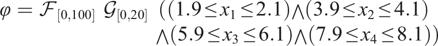
Recurring tasks
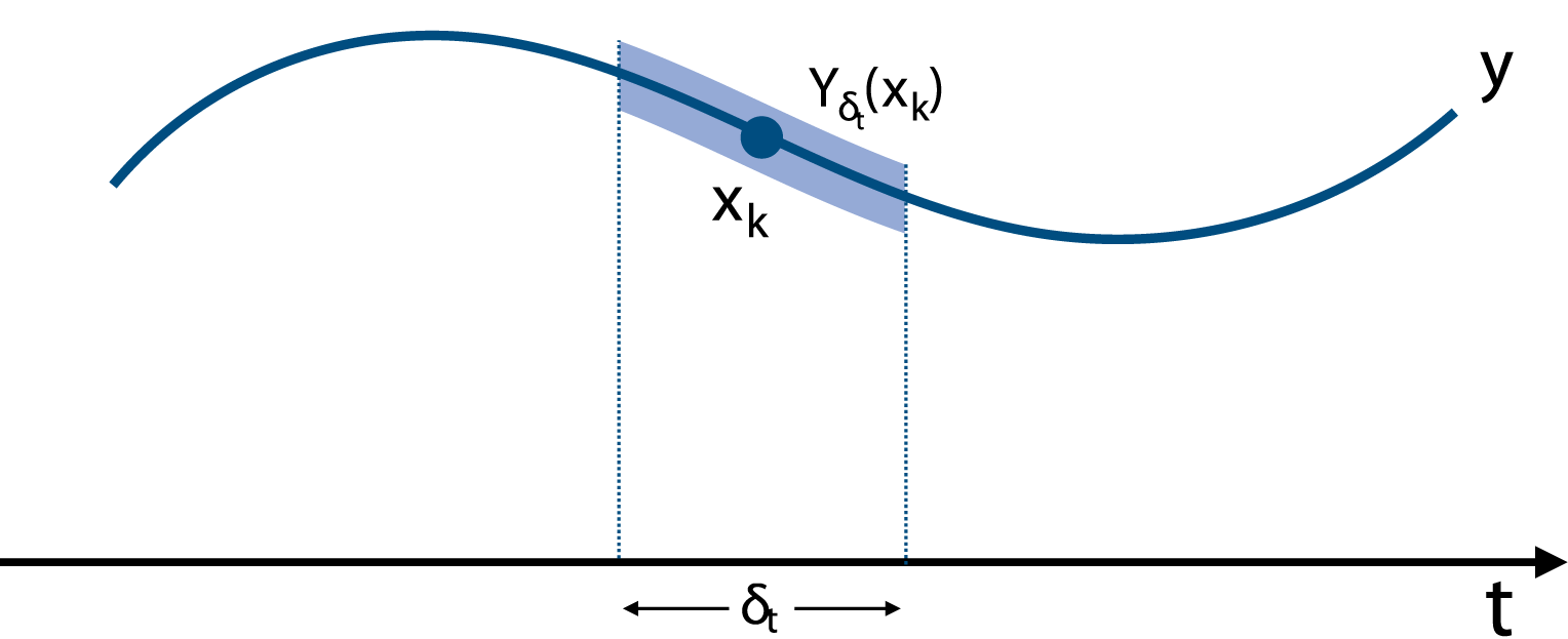
The next scenario is that of recurring tasks. This can be useful when an autonomous vehicle needs to repeatedly survey an area at regular intervals, a bipedal robot needs to plan periodic foot movements, or a ground robot needs to visit a charging station at specified intervals. The STL formula to express such requirements is given by 
In reference to Remark 2, an example of post-processing the trajectories is shown in Figure 7 for the STL formula, Simulation results of MAPS2 with four agents
Multi-agent case study
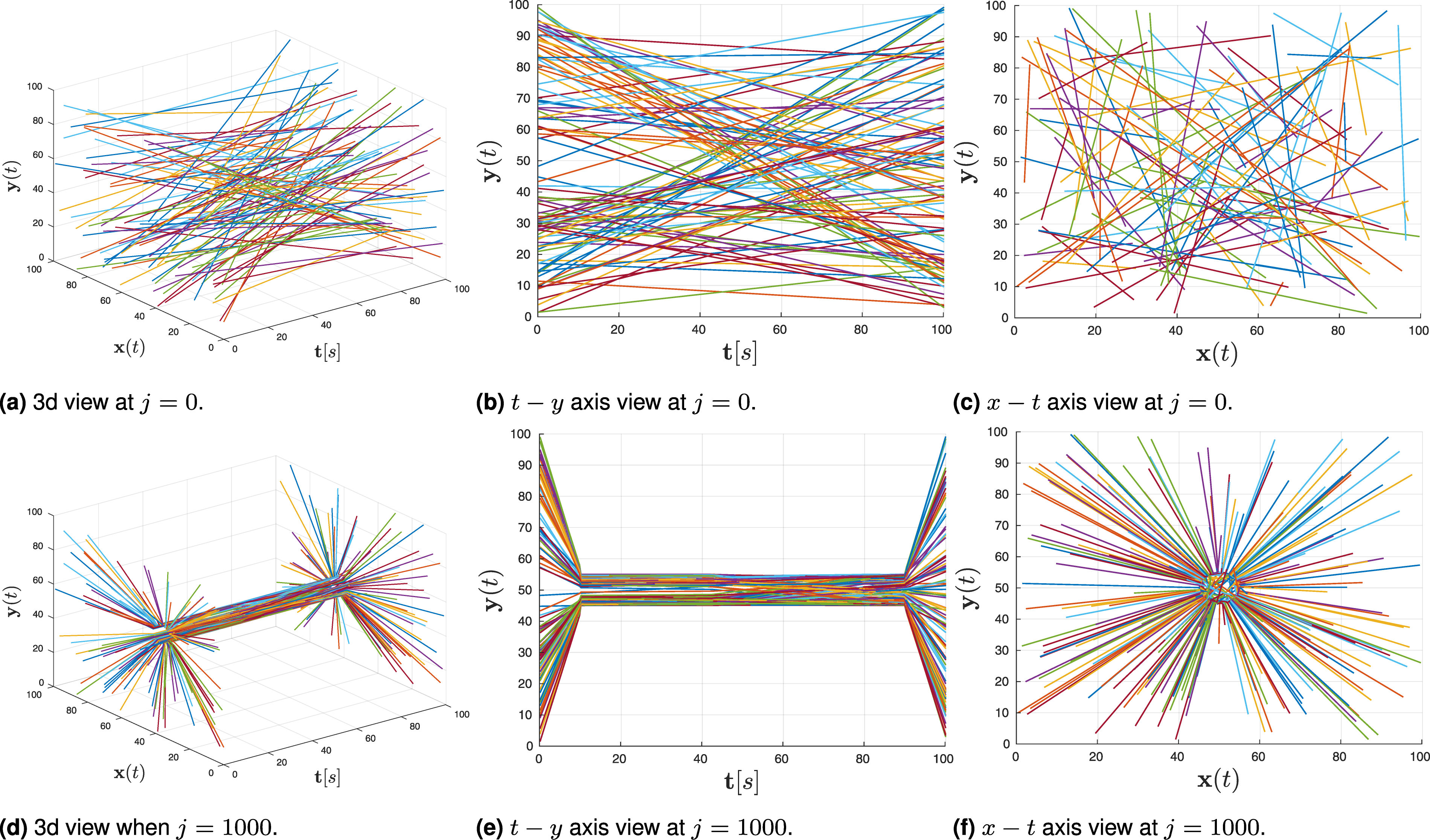
In this case study, we design trajectories for a team of 100 agents that exist in a 100 × 100[m] space and [0,100][s] time span. The team needs to adhere to the following STL formula, Non-smooth and smooth paths for the formula (10). Simulation of trajectory generation for 100 agents for the STL formula (11).
Overall case study
In this case study, we demonstrate the application of the aforementioned scenarios by setting up the following tasks: • Agent 1 always stays above 8 units. • Agents 2 and 4 are required to satisfy the predicate • Agent 3 is required to track an exponential path within the time interval [20,60][s]. • Agent 2 is required to repeatedly visit Agent 1 and Agent 3 every 10 s within the interval [30,50][s]. • Agent 1 is required to maintain at least 1 unit distance from the other three agents within the interval [80,100][s].
The STL formula for the above tasks is as follows: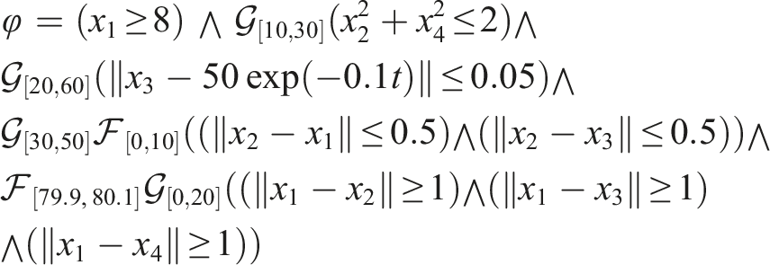
The parameter L was increased to 1000, and η was decreased to 0.001. In Figure 10, we show the resulting trajectories of each agent generated by Robustness of the STL formula in (11).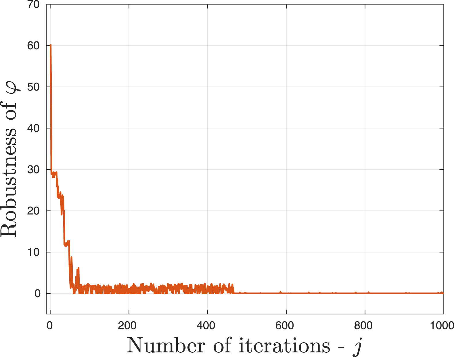
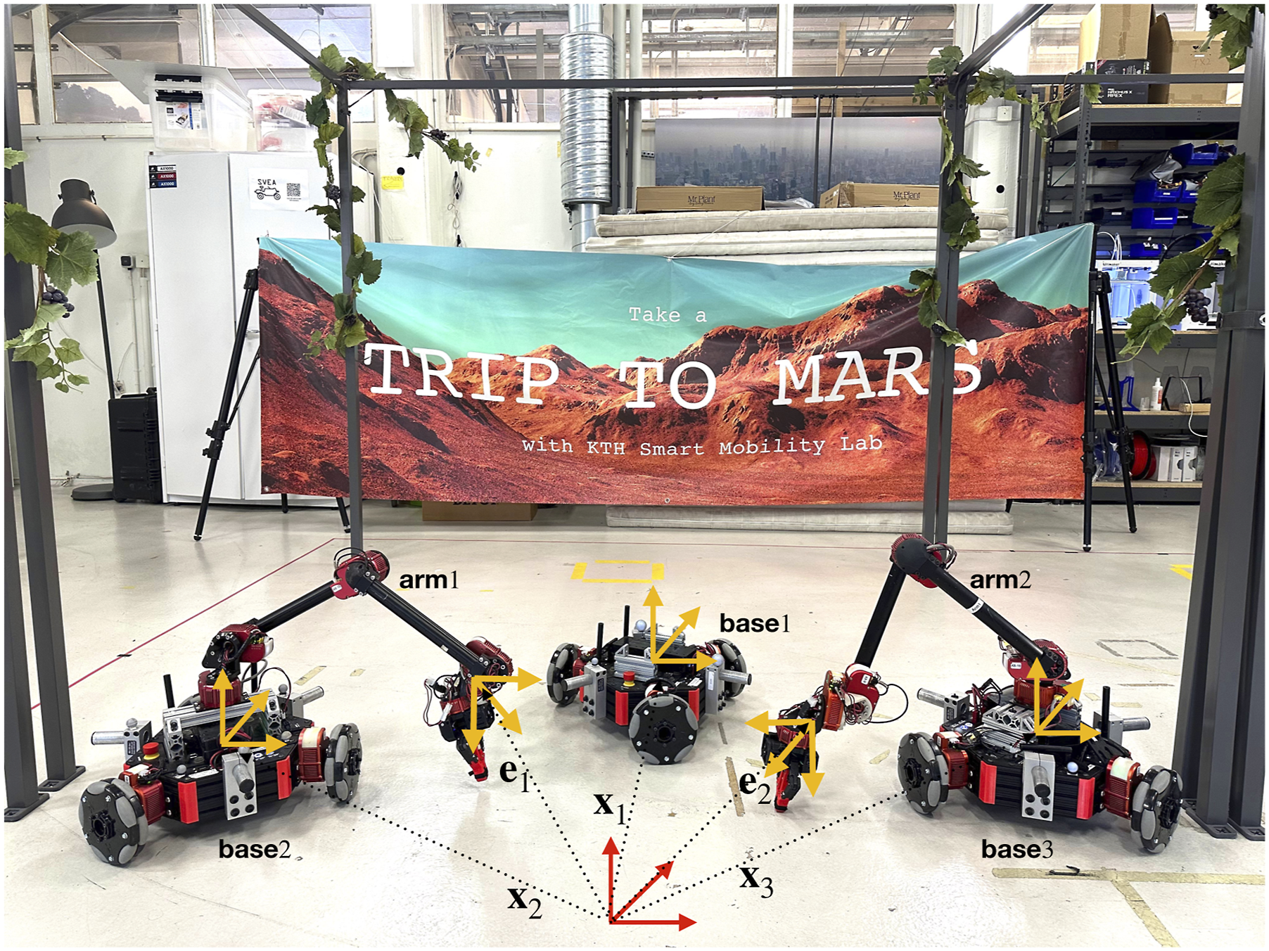
Experiments
We now present an experimental demonstration of the proposed algorithm. The multi-robot setup involves three robots, as shown in Figure 11, and consists of 3 mobile bases and two 6-DOF manipulator arms. The locations of the three bases are denoted as Overall case study. Experimental setup with three mobile bases and two 6-dof manipulators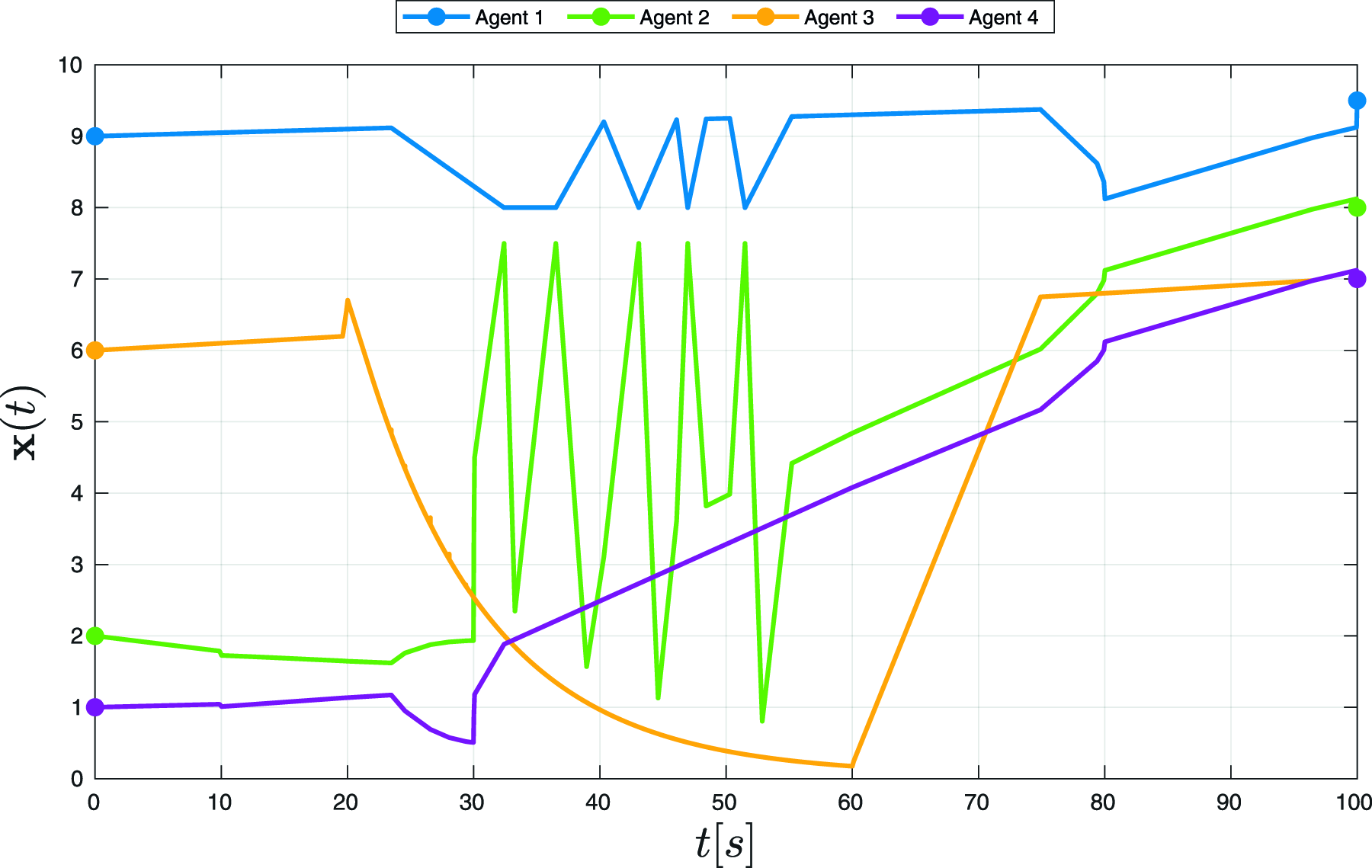
The STL formula defining the tasks is the following,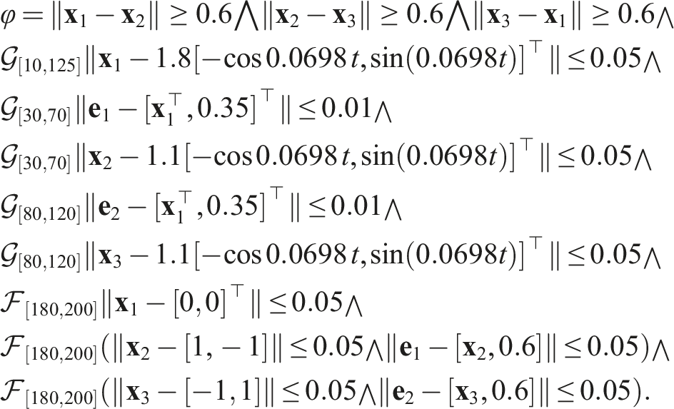
The above task involves collision avoidance constraints that are always active given by the subformula
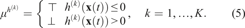
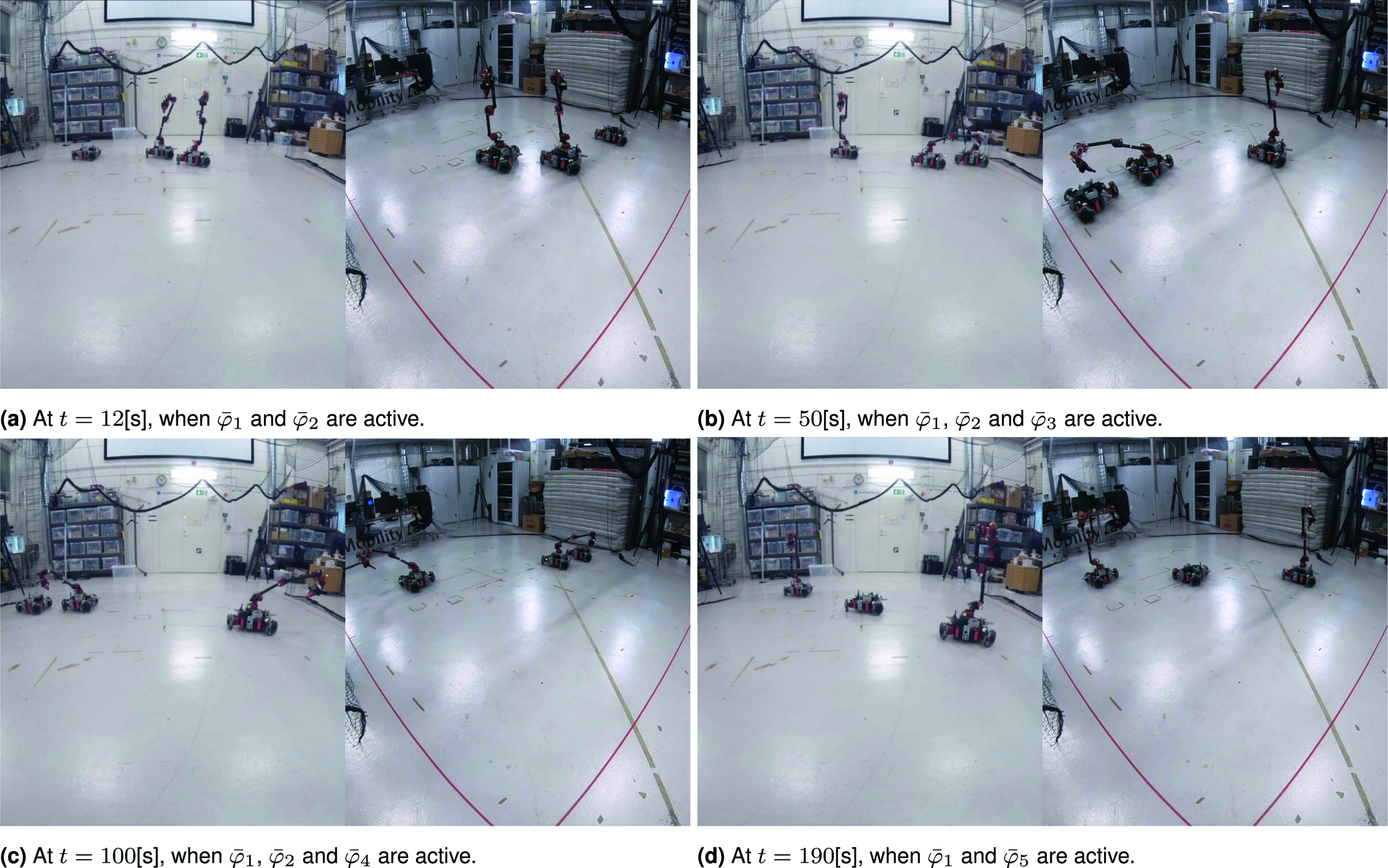
The results are shown in Figure 12, where the x-axis represents time in seconds, and the y-axis represents the predicate functions defined by (5). The dashed line in the plots represents the predicate functions of the trajectories obtained by solving the optimisation problem (8), while the solid line represents the predicate functions of the actual trajectories by the robots. In the context of (5), negative values indicate task satisfaction. However, due to the lack of an accurate model of the robots and the fact that the optimisation solution converges to the boundary of the constraints, the tracking is imperfect, and we observe slight violations of the formula by the robots in certain cases. Nonetheless, the trajectories generated by the algorithm do not violate the STL formula. The coloured lines represent the functions that lie within the validity domain of the formula. Figure 12(a) shows that the collision constraint imposed on all 3 bases is not violated, and they maintain a separation of at least 60 cm. In Figure 12(b), base 1 tracks a circular trajectory in the interval [10, 125] seconds. In Figures 12(c) and 12(d), the end effectors mounted on top of bases 2 and 3 track a virtual point over the moving base 1 sequentially. In the last 20 seconds, the bases and end effectors move to their desired final positions, as seen in Figures 12(e) and 12(f). The maximum computation time by any robot is 3.611[s]. Figure 13 shows front-view and side-view at different time instances during the experimental run.
3
Experimental verification of MAPS2 with the setup in Figure 11. Front-view and side-view during experimental run with the setup in Figure 11.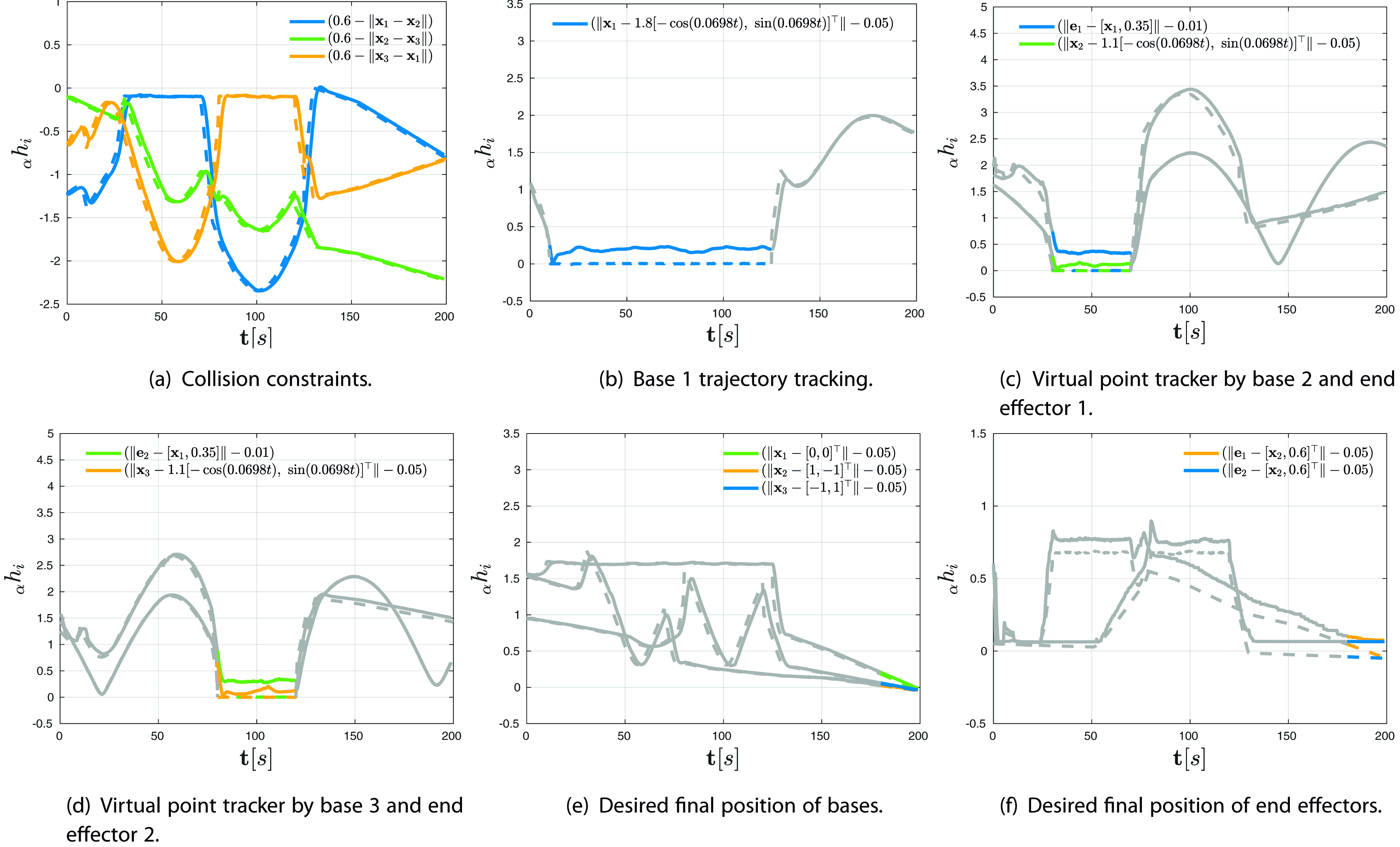
Conclusion
This work proposed MAPS2, a distributed planner that solves the multi-robot motion-planning problem subject to tasks encoded as STL constraints. By using the notion of validity domain and formulating the optimisation problem as shown in (8), MAPS2 transforms the spatio-temporal problem into a spatial planning task, for which efficient optimisation algorithms already exist. Task satisfaction is probabilistically guaranteed in a distributed manner by presenting an optimisation problem that necessitates communication only between robots that share coupled constraints. Extensive simulations involving benchmark formulas and experiments involving varied tasks highlight the algorithms functionality. Future work involves incorporating dynamical constraints such as velocity and acceleration limits into the optimisation problem.
Supplemental Material
Footnotes
Funding
The authors disclosed receipt of the following financial support for the research, authorship, and/or publication of this article: This work was supported by the ERC CoG LEAFHOUND, the Swedish Research Council (VR), the Knut och Alice Wallenberg Foundation (KAW) and the H2020 European Project CANOPIES.
Declaration of conflicting interests
The authors declared no potential conflicts of interest with respect to the research, authorship, and/or publication of this article.
Supplemental Material
Supplemental material for this article is available online.
Notes
References
Supplementary Material
Please find the following supplemental material available below.
For Open Access articles published under a Creative Commons License, all supplemental material carries the same license as the article it is associated with.
For non-Open Access articles published, all supplemental material carries a non-exclusive license, and permission requests for re-use of supplemental material or any part of supplemental material shall be sent directly to the copyright owner as specified in the copyright notice associated with the article.