
Abstract
Seafloor surveys often gather multiple modes of remote sensed mapping and sampling data to infer kilo- to mega-hectare scale seafloor habitat distributions. However, efforts to extract information from multimodal data are complicated by inconsistencies between measurement modes (e.g., resolution, positional offsets, geometric distortions) and different acquisition periods for dynamically changing environments. In this study, we investigate the use of location information during multimodal feature learning and its impact on habitat classification. Experiments on multimodal datasets gathered from three Marine Protected Areas (MPAs) showed improved robustness and performance when using location-based regularisation terms compared to equivalent autoencoder-based and contrastive self-supervised feature learners. Location-guiding improved F1 scores by 7.7% for autoencoder-based and 28.8% for contrastive feature learners averaged across 78 experiments on datasets spanning three distinct sites and 18 data modes. Location-guiding enhances performance when combining multimodal data, increasing F1 scores by an average of 8.8% and 37.8% compared to the best-performing individual mode being combined for autoencoder-based and contrastive self-supervised models, respectively. Performance gains are maintained over a large range of location-guiding distance hyperparameters, where improvements of 5.3% and 29.4% are achieved on average over an order-of-magnitude range of hyperparameters for the autoencoder and contrastive learners, respectively, both comparing favourably with optimally tuned conditions. Location-guiding also exhibits robustness to position inconsistencies between combined data modes, still achieving an average of 3.0% and 30.4% increase in performance compared to equivalent feature learners without location regularisation when position offsets of up to 10 m are artificially introduced to the remote sensed data. Our results show that the classifier used to delineate the learned feature spaces has less impact on performance than the feature learner, with probabilistic classifiers averaging 3.4% higher F1 scores than non-probabilistic classifiers.
Keywords
1. Introduction
Understanding kilo-hectare scale seafloor habitat distributions is a basic requirement for statutory monitoring and scientific advance. Due to the complexity of habitats, traditional workflows require many aspects of environmental data to be measured and then interpreted by human experts to infer habitat class and distribution (Verfaillie and Van Lancker, 2008). Figure 1 illustrates typical approaches for gathering environmental data. Multibeam echo sounder (MBES) surveys are used to gather seafloor depth information and generate bathymetry maps, where some systems also record the acoustic reflection intensity, or backscatter, that helps to determine seafloor substrate, where hard substrates like rock or coarse sand have higher acoustic reflectivity than softer sediments like silt and clay. Side scan sonar (SSS) also measures seafloor acoustic backscatter, achieving a large swath and higher resolution than MBES backscatter measurements when made from the same range. For shallow seafloors (<200 m), acoustic instruments can be used directly from ships to achieve the metre-order resolution needed to identify habitat characterising features. In deeper water, these instruments need to be mounted on ship-towed submersibles or Autonomous Underwater Vehicles (AUV) to achieve sufficient resolution (Brown et al., 2011). In very shallow, clear water (<30 m), satellite images (SI) and aerial images (AI) can also provide valuable information about seafloor appearance over wide areas (Ohlendorf et al., 2011; Price et al., 2022). The direct parametrisation of habitats from metre-resolution data is non-trivial, and typically multiple layers of remote sensed mapping data are correlated with habitat information derived from higher-resolution surveys conducted in some portion of the mapped region. Both physical samples recovered from the seafloor and millimetre-resolution visual imagery (Yamada et al., 2021b) provide information from which habitat classes can be directly derived. Inferred relationships between the remote sensed priors and observation-derived classes can then be used to predict habitat distributions in unobserved parts of the remote sensed data. Overview of kilo-hectare scale seafloor mapping methods (left) and the proposed multimodal inference scheme (right). Satellite and airborne cameras can obtain visual images of benthic habitats in clear shallow water (<30 m) and shipboard side scan sonar (SSS) can gather wide area acoustic backscatter intensity data for seafloor depths of up to 200 m. Shipboard multibeam echo sounders (MBES) can gather bathymetry information in both shallow and deep water, but with resolution decreasing with depth. Higher resolutions can be achieved for deep seafloors using SSS and MBES equipped Autonomous Underwater Vehicles (AUVs). The data gathered using these methods provide some information about habitats but require overlapping sampling to identify specific habitat types, and so can be considered as priors. AUVs equipped with cameras can efficiently gather visual images in which some habitat types can be identified. As shown in the bottom right figure, various types of habitats are depicted in distinct colours. The class of these habitat patches can be ascertained by employing a voting mechanism based on AUVs’ observations. The multimodal inference concept illustrated to the right shows multiple prior map layers being fused, using location metadata to regularise self-supervised feature learning. AUV visual images provide habitat observations that can be used to train and validate habitat inference onto multimodal features extracted from the priors.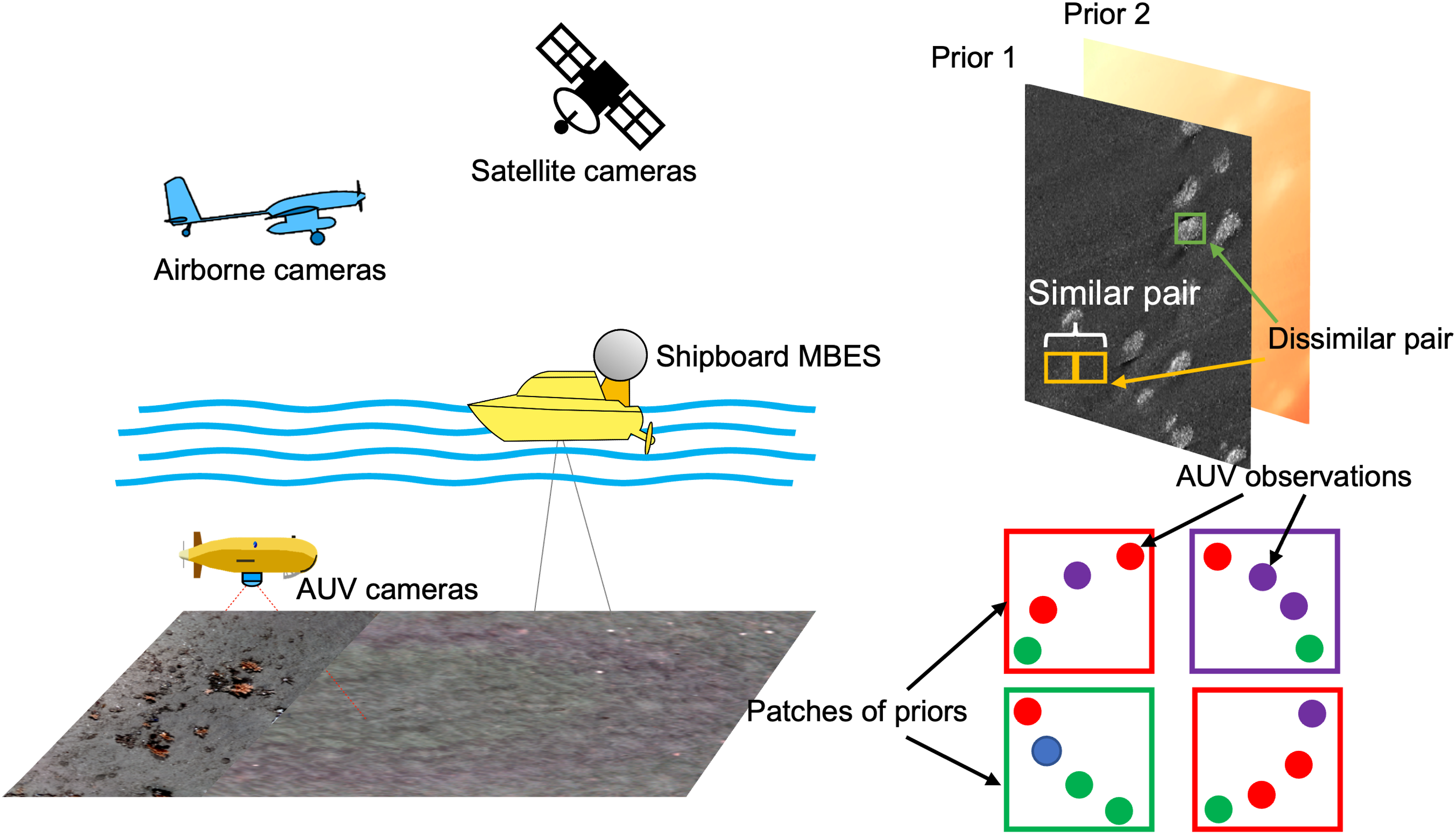
Utilising multimodal data is common in habitat classification. For example, Zelada Leon et al. (2020) considered multiple remote sensed priors for automated habitat classes inference, where feature extraction was performed on individual data modes and then later combined. In Rao et al. (2017), features were simultaneously extracted from a prior map and overlapping in situ observations. Besides, Shields et al. (2020) extended this approach and investigated how to address the different footprints of remote sensed priors and in situ data. However, methods to combine multiple priors during feature extraction and the impact of inconsistencies between data modes, such as positional offsets, shape discrepancies and for dynamic environments different acquisition times, are not well understood. Other barriers, for example, data imbalance due to the uneven distribution and extent of different types of habitats, also need to be considered. To address these challenges, this paper investigates the impact of using location metadata during feature learning for improved prediction of habitat distributions in remote sensed mapping data. We compare the performance of two approaches of incorporating location metadata to equivalent methods. The first approach is the location guided autoencoder, which is an AlexNet-based autoencoder that incorporates a soft-location constraint to regularise learning (Yamada et al., 2021b). We compare this to an equivalent AlexNet-based autoencoder that does not use location metadata. The second approach is a georeferenced contrastive learner, implemented using ResNet-18 that incorporates a hard-location metadata based constraint to regularise learning (Yamada et al., 2022). We compare this to an equivalent ResNet-18 trained using a contrastive learning method that does not use location metadata. Specifically, the following contributions are made: • Developing a method for wide area substrate and habitat classes (facies) predictions by learning features from multiple remote sensing data modes and inferring relationships to classes derived from overlapping in situ imagery. • Investigating the use of location metadata to improve feature learning for both single mode and multimodal remote sensing data, and maintain the robustness to combinations with data modes that have poor information content. • Investigating the robustness to practical issues of position offsets between data modalities and the sensitivity of the method to hyperparameter tuning during location-based regularisation.
The method advances marine perception by enabling machines to interpret multiple layers of prior information about their environment together with their observations. This can inform robotic action by improving their ability to make intelligent decisions, for example, in informative path planning for more targeted or evenly distributed observation of various seafloor habitat types.
The remainder of the paper is arranged as follows: Section II provides a review of related works in data acquisition, feature learning and multimodal inference, identifying current limitations. Section III presents our multimodal inference workflow, which uses self-supervised learning with location-based regularisation when extracting combined features from multiple input modalities. Section IV presents experiment results and analyses conducted on three field survey datasets. Section V presents our conclusions.
2. Literature review
2.1. Seafloor data acquisition
Data from multiple sources can be used for benthic habitat classification (see Figure 1). These can be broadly split as follows: • Remote sensed mapping priors • Sampling and in situ camera observations
Remote sensing mapping methods can seamlessly cover spatial extents of several kilo-hectares to kilometres squared. Examples include acoustic bathymetry from MBES providing depth information, and the backscatter intensity from SSS and MBES illustrating the hardness of substrate. Satellite images (SI) and aerial images (AI) taken by satellites and airborne cameras can also show the visual appearance of the seafloor in shallow water. The resolution of such data modes varies between tens of centimetres to tens of metres depending on acquisition conditions but is typically insufficient to directly determine substrate and habitat types without some separate form of observation.
Substrate and habitat classes can be directly identified through recovery of physical samples or high-resolution images. Sampling is an inherently destructive process and is also time-consuming where typically gathering tens to just over a hundred samples to characterise a region (Neettiyath et al., 2021; Usui et al., 2017). Seafloor visual imaging is a non-destructive process. But due to the strong attenuation of light in water, seafloor visual imaging requires the use of artificial lighting and cameras that are operated within a few metres above the seabed (Bodenmann et al., 2017). Even with high-altitude imaging setups, observational footprints are limited to <100 hectares per 24 h of observation (Thornton et al., 2021). However, the high resolution of imaging surveys (<1 cm) makes them suitable for identifying different types of seafloor habitats, substrata and species. Several prior works have demonstrated semi-supervised classification of seafloor imagery achieving high F1 accuracy scores (Ojala et al., 2002; Yamada et al., 2022).
A major challenge for large-scale seafloor habitat characterisation is the large gap between the extent covered by remote sensing and sampling or in situ camera observations. Remote sensing datasets cover vast regions at high-resolution, they can have measurements across many channels and the same geo-location can be described using multiple sensing modalities. Managing the resulting high-dimensionality is challenging for direct use of classifiers, and various approaches have been investigated to reduce dimensionality while retaining information that is useful for habitat interpretation. To efficiently identify boundaries between the different classes in a mapped region, automated interpretation methods often first project remote sensed data to a lower-dimensional feature space that aims to retain sufficient information while reducing information redundancy.
2.2. Feature extraction
Methods for feature extraction fall into two categories (Yamada et al., 2021b): • Feature engineering, where features designed by humans are manually selected and combined • Feature learning, where features are algorithmically identified through an optimisation process
In feature engineering, Grey Level Co-occurrence Matrices (GLCMs) were first proposed in Haralick et al. (1973) as an effective and generalisable method for textural feature extraction. GLCMs combine image-derived features such as contrast and correlation to provide compact representations of grey-scale images. Zelada Leon et al. (2020) used 64 GLCM features and investigated the accuracy and repeatability of various methods for seafloor habitat classification. Fanlin et al. (2021) combined five GCLM features and angular response curves to represent acoustic images for seafloor classification. Scale-Invariant Feature Transform (SIFT) (Lowe, 1999) is an alternative to GLCMs that is extensively used to extract features from images. SIFT identifies points within an image where the intensity stands out from the local neighbourhood over different spatial scales. The distribution of these points forms a set of features that can be used to describe the image. Speeded-Up Robust Features (SURF) were developed to improve the SIFT by using optimised integral operations (Bay et al., 2006). Other forms of textural features include Local Binary Patterns (LBPs), which encode local relationships between the central pixel and its neighbouring pixels (Ojala et al., 2002). While engineered features have proven to be highly effective across a wide range of tasks, their performance may degrade under challenging conditions, such as in low-contrast or non-rigid scenes. Additionally, some methods, such as GLCMs, still require feature optimisation through combinations, which can be inconvenient to process multiple datasets.
Feature learning eliminates the need for manual optimisation and selection of predefined features. Instead, it leverages learning techniques to automatically extract features that efficiently describe a training dataset. Convolutional neural networks (CNNs) are widely used to flexibly learn representations of features directly from images, without the need for explicit feature engineering. The principle of deep CNNs has been analysed theoretically in Wiatowski and Bölcskei (2017) and many CNN architectures and training methods have been developed and applied to feature extraction and image classification tasks. AlexNet, proposed by Hinton et al. (2012), demonstrated that an increased number of layers in the network architecture enabled more complex feature representations, outperforming shallow networks in benchmarking studies. Later, deeper network architectures such as VGGnet (Simonyan and Zisserman, 2014) and Residual Network (ResNet) (He et al., 2016) were proposed and showed further improvements for classification tasks. A drawback of larger networks is the increased computational cost for network training, and CNNs such as MobileNet have attempted to reduce the number of parameters within the CNN architecture (Howard et al., 2017), for use in applications where computing resources are limited, for example, mobile robotic and sensing applications. Similar efforts have investigated the structure of CNNs to achieve efficient scaling of architectures (EfficientNet) for optimised performance under different computational constraints (Tan and Le, 2019). Recently, CNNs have been applied for automated interpretation of seafloor data. Mahmood et al. (2018) classified images of coral into nine classes, demonstrating the potential of CNNs to model habitats according to taxonomic class boundaries used in conservation ecology. However, a drawback of using CNNs is that traditional supervised learning approaches require large volumes of human-labelled training data to achieve accurate results. This is because the supervised classifiers simultaneously learn image descriptors (i.e., latent representation spaces) and delineate class boundaries in a single training process. The former requires hundreds to thousands of labelled instances for effective training, which is limiting since generating human-labelled data is time-consuming. Transfer-learning attempts to limit the number of domain-specific human-labelled training instances by first training CNNs on large, generic image datasets (Deng et al., 2009; Everingham et al., 2010; Lin et al., 2014), and then fine-tuning networks based on a smaller number domain-specific training data (Weiss et al., 2016). However, the performance of this approach is limited when the appearance of data in the target domain differs from the training repositories (Yamada et al., 2023).
Self-supervised learning has achieved state-of-the-art performance by separating the processes of feature learning and delineation of the learned feature space through semi-supervised classification (Chen et al., 2020a). Self-supervision trains CNNs to learn the features that best describe a dataset without the need for human-labelled datasets, which is an advantage because unlabelled datasets are more numerous and accessible. Instead, these approaches optimise CNNs parameters based on intrinsic structures that exist within unlabelled datasets (Chen et al., 2020a, 2020). Self-supervised learners attempt to map similar instances of data to the same region of a latent representation, or feature space, making them robust to small input or network weight perturbations (Samuli and Timo, 2017). Typically, artificially perturbed instances of the same sample are provided as pairs to the CNNs, where model weights are tuned so that the predictions (i.e., latent representation) are similar across the perturbations (Preciado-Grijalva et al., 2022). Self-supervised training methods have also been developed to pair different samples that are likely to have similar appearances based on certain rules. Yamada et al. (2022, 2021b) introduced a distance parameter when processing seafloor visual image datasets, where seafloor images that were taken close to each other were assumed to share similar properties since the footprint of an image is relatively small to the broader changes in seafloor substrates and habitats. Although this assumption will not always be satisfied, for example, near habitat transition areas, previous studies (Grant et al., 2024; Yamada et al., 2021b) showed that the approach is robust as long as the visual characteristics generally change over spatial scales larger than the distance parameter used.
Semi-supervised classifiers use intrinsic structures in the learned latent-representation space (Yamada et al., 2022, 2023) to reduce the number of labelled instances needed to delineate human class boundaries. In addition, this also reduces the susceptibility to human bias during training. For instance, Bijjahalli et al. (2023) developed a self-supervised learning framework based on variational autoencoders (VAE) to detect artificial objects in underwater imagery. The method applies clustering to the latent representation space and identifies samples that are distant from cluster centres. These images were considered anomalous and potentially showing artificial objects. Semi-supervision through human confirmation of artificial objects further improved learning performance. In order to avoid overfitting a small set of human-labelled data, several studies have investigated machine-guiding to identify samples for human-labelling based on the distribution of data in the latent representation space. For instance, Yamada et al. (2023) achieved 85% of the classification accuracy of an equivalent supervised CNN trained with 10,000 expert labels, using just 40 machine-guided labels. The approach used hierarchical K-means sampling to identify cluster representative images in the latent representation space, where algorithmically selected representative images improved the performance of classifiers compared to an equivalent number of randomly selected images. This approach was also found to improve performance under class imbalance by selecting the same number of images from each cluster found in the data.
2.3. Multimodal data interpretation
Combining different sensing modalities that capture diverse aspects of a measurement target has the potential to improve classification performance, and has been investigated in many applications, including seafloor habitat mapping (Rao et al., 2017), agriculture (Kang et al., 2023) and facial recognition (Nandi et al., 2022). Various approaches have been demonstrated, where these can be broadly grouped as early fusion, late fusion and middle fusion (Boulahia et al., 2021; Hong et al., 2020).
Early fusion merges raw or pre-processed sensor data before feature extraction. This ensures that joint features can be captured from multiple modalities at the onset of training, maximising the information derived from multimodal datasets (Cui et al., 2021; Gadzicki et al., 2020). A limitation of early fusion is an inherent sensitivity to spatial or temporal misalignment, which can arise from sensor resolution mismatches, geometric distortions, or changes in the environment between the acquisition of the different data modes. Boulahia et al. (2021) proposed early fusion to combine RGB images, depth maps and skeletal sequences for recognition of human actions. To address resolution mismatches between data modes, depth maps were resized to match RGB image sizes prior to feature extraction for downstream classification. Early fusion was also used to combine visual and thermal images for improved weed detection in agricultural applications (Zamani and Baleghi, 2023), where pre-processed visual images and thermal images were directly stacked ahead of feature extraction. In Jain et al. (2022), the authors demonstrated early fusion with contrastive self-supervised learning to interpret different satellite imaging modalities as similar pairs from the same geographic location. The results showed improved performance compared to a single mode when using multiple modalities. However, positional and geometric inconsistencies in satellite images are relatively limited compared to the remote sensing modes used in the marine domain, where different measurement physics and observation ranges are used, with inherent limitations in subsea positioning accuracy (Paull et al., 2014). Another factor is the longer time intervals between data acquisition due to mobilisation and survey logistics of marine operations, where even well-studied regions of the seafloor may only be visited once a year or less. The impact of these intermodal inconsistencies on multimodal learning is not understood.
Late fusion approaches combine the outputs from classifiers that are tailored to each sensing modality using a decision tree (Maki et al., 2011) or combine features derived from individual modalities by concatenating, or down-selecting a mixture of informative features as inputs for a classifier (Neettiyath et al., 2021; Takahashi et al., 2023). Advantages are that this approach is modular, where the introduction of new sensing modalities and corresponding mode-specific feature extractors does not impact other sensing modes, and there is flexibility as both feature engineering (Maki et al., 2011; Neettiyath et al., 2021) and feature learning (Takahashi et al., 2023) can be used. This approach can address issues of resolution mismatch that are common in remote sensing data as the feature extraction process can be coordinated between data modes. However, this also limits scalability as each data mode increases the computation cost and memory requirements. In addition, intermediate features that are potentially beneficial for classification may be missed, and conversely features from data modes that do not provide useful information can introduce noise into the final classification result. In Gunes and Piccardi (2005), the authors studied visual emotion recognition from facial expressions and body gestures, fusing the modalities at the decision level. Although the comparison experiments revealed that the early fusion method achieved higher classification accuracy, the late fusion made the feature extraction more flexible, where models for one modality can also be directly used in future tasks or recombined with other modes without re-training.
Middle fusion takes features that are individually extracted from each sensing modality and uses mathematical operations to derive a new set of features that express multimodal information. The distinction from late fusion is that the features used for classification are not a subset or combination of features extracted from each data mode, but instead features that individually contain information from multiple sensing modes. This approach maintains the flexibility of late fusion while allowing redundant information to be removed before classification. The method to fuse features from different modes is an actively researched area, where studies have demonstrated Bayesian optimisation (Ramachandram et al., 2017), genetic algorithms (Whitley et al., 1990), principal component analysis (Zelada Leon et al., 2020) and t-distributed Stochastic Neighbor Embedding (t-SNE) (Takahashi et al., 2023). In the study of Rao et al. (2017), features from visual images and bathymetry were extracted separately in a gated deep-learning architecture and then an intermediate shared layer was constructed to perform data fusion. The intermediate shared layer contains features of both the visual image dataset and bathymetry so that it is capable of predicting visual image and bathymetric features. In Takahashi et al. (2023), features derived from chemical signatures and holographic images of marine particles were combined using t-SNE. A comparison with late fusion, where the features derived from chemical signatures and imagery were concatenated, showed improved classification accuracy with t-SNE-based middle fusion, demonstrating the advantage of being able to recompute features based on multimodal inputs. Karpathy et al. (2014) compared early, late and middle fusion in the study of large-scale video classification, where a low-resolution context stream and a high-resolution fovea stream (i.e., images with non-uniform resolution, optimised based on some image region criteria) were fused in different ways. The result revealed that the middle fusion performed better than early and late fusion for this application (Feng et al., 2020). However, studies have found that the performance of these approaches is sensitive to data modalities, classification targets and network architectures (Feng et al., 2020), with no consensus being reached that any one approach consistently outperforms the others.
For benthic habitat classification, early fusion has the advantage that it can fully consider the information given by multiple modalities while remaining computationally efficient since only a single feature extractor and classifier are needed. However, early fusion is potentially more sensitive to data inconsistencies than late and middle fusion. Although methods such as resampling can be used to address the resolution mismatch, inconsistencies such as geometric distortion, positional offsets, and changes in the environment between the acquisition of different modes still exist. Although approaches to improve consistency across data layers exist, we argue that such spatial and temporal inconsistencies are inherent between seafloor mapping modalities, and so it is valuable to understand their impacts and develop robust approaches that minimise performance degradation.
2.4. Classification
In order to evaluate the feature learning performance, it is imperative to train a classifier to derive the ultimate predictive class labels. A significant challenge encountered during this process is data imbalance, a prevalent issue due to the heterogeneous distribution of habitats on the seafloor, resulting in imbalanced observations of AUVs. To address this, recent methodologies have been developed, focusing on rectifying data imbalance. These include strategies such as under-sampling and over-sampling (He and Garcia, 2009), along with algorithmic approaches like boosting (Singh and Purohit, 2015) and bagging (Hasib et al., 2020). Resampling techniques aim to equalise the representation of data classes by either augmenting or diminishing the number of samples. Conversely, boosting and bagging enhance training effectiveness through methods such as the utilisation of sub-datasets for repeated training and the aggregation of multiple weak classifiers to fortify the overall strength of the model. In this study, we deploy the SMOTE (synthetic minority over-sampling technique) (Fernández et al., 2018), a specific method in resampling techniques, to deal with the data imbalance problem owning to its easier implementation and low computation load compared to other strategies (Chawla et al., 2002).
Labelled visual image datasets are utilised to establish the ground truth through geo-registration processes. However, the footprint of these visual images, denoted as
Deep learning techniques are also often used for direct classification. Both CNNs (Chaganti et al., 2020; Lee and Kwon, 2017) and transformers (Bhojanapalli et al., 2021) can be used to encode images into a feature space, where a MLP (multi-layer perceptron) can be added after these to predict class labels. Recently, transformers have demonstrated state-of-the-art performance in classification tasks (Han et al., 2022). Typically such approaches are trained directly through supervised learning. However, this requires large and well curated datasets (Zhou et al., 2021). Given the challenges of creating such a dataset for diverse marine habitats, supervised CNNs and transformer-based classifiers are not explored in this paper.
3. Method
Multimodal data has the potential to improve the accuracy and robustness of habitat classification as diverse sensing modalities can probe different aspects that characterise an environment. The key stages of our approach include: • Fusing multiple prior layers: Combine multiple remote sensing data layers to generate a rich representation of the seafloor. • Feature learning with location metadata: Enhance feature extraction by leveraging location metadata to regularise learning. • Geo-registration for correlating visual class information: Addressing the different spatial extents of image derived visual habitat classes and the seafloor representations generated from remote sensed priors. • Visual habitat class inference: Training machine learning models to predict visual habitat class distributions and their prediction uncertainty over large spatial extents.
The proposed multimodal inference pipeline is illustrated in Figure 2. We investigate the impact of location based regularisation of the latent representation space, and the impact of combining multiple remote sensed priors. We also investigate the robustness of performance to data inconsistencies. Overview of the seafloor habitat classification method. The grey blocks indicate processes. Self-supervised learning is applied to overlapping patches of the multimodal priors to obtain a latent representation space, or feature space, of the fused remote sensing data. In training, location metadata is used to regulate feature space distances, where geographically closer pairs are placed closer in the feature space compared to equivalent training methods that don’t use location metadata, and geographically distant pairs are left far apart. This constraint prioritises patterns that are found to recur in nearby patches, which can help capture habitat relevant characteristics. Features extracted from multimodal remote sensing data can be correlated with visual habitat classes generated from AUV camera observations in the same region, where we address the mismatch between remote sensing patch size and the footprint of visual images by determining class proportions. The correlation between visual class proportion and patch extracted features is used to infer habitat distributions over a large extent.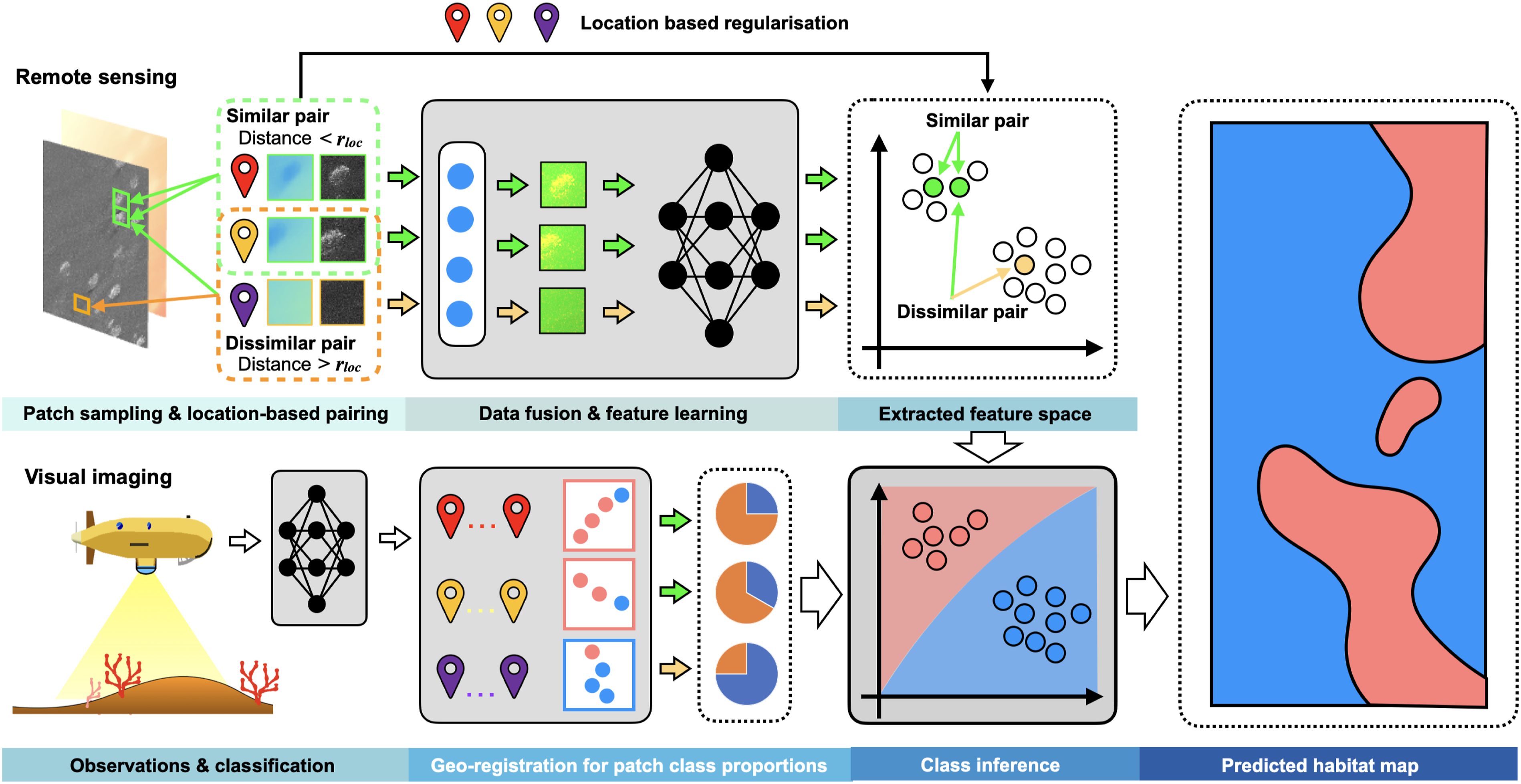
Mapping seafloor substrate and habitat class distributions requires spatial patterns larger than the resolutions of remote sensed mapping data (typically in the order of tens of centimetres to several metres) to be captured. Although localisation uncertainties exist in seafloor mapping applications, these are of a similar order of magnitude to the resolution of remote sensed mapping data, ranging from metres to tens of metres with standard navigational suites (Paull et al., 2014). Since substrates and habitats usually cover spatial extents that are several orders of magnitude larger than the resolution of remote sensed prior maps, it is possible to make the following assumption (Koenig, 1999; Tobler, 1970):
Although patchy features and transitions between habitats can cause the assumption to be locally unsatisfied, previous studies have shown that the assumption improves results compared to methods that do not use location information (Yamada et al., 2021b; Grant et al., 2024). In addition, disturbance events and gradual changes in the environment may also affect the distribution of habitats, in most practical situations the above assumption can still be made without loss of generality. The proximity assumption can be applied across data modes because different sensing modes capture diverse aspects of the underlying substrates and habitats at each location. For feature extraction, we take two self-supervised learning frameworks that have been adapted to take advantage of location metadata and have been shown to be effective for the classification of seafloor imagery. The Location-Guided Autoencoder (LGA) applies a soft location constraint to regularise feature learning through modification of the autoencoder cost function and was shown to improve the quality of features extracted from seafloor images compared to a regular autoencoder (Yamada et al., 2023). Georeferenced Contrastive Learning of Visual Representations (GeoCLR), on the other hand, applies a hard location constraint by selecting nearby images as similar pairs in contrastive learning. We extend these methods to perform multimodal feature learning using early fusion by integrating raw data from multiple remote sensed priors. The feature space is then correlated against classes derived from in situ seafloor imagery in spatially overlapping regions. We compare probabilistic and non-probabilistic approaches to delineate the visually derived class boundaries in the feature space of the remote sensed priors, in order to fully evaluate the performance of the proposed self-supervised learning frame. The method allows the visually derived class distribution to be predicted over the entire remote sensed region, covering significantly larger areas than what is feasible to image directly. Our investigation compares results with feature learners that do not use location metadata and investigates the effects of positional inconsistencies between data modes.
3.1. Convolutional early fusion
We leverage the proximity assumption to perform early data fusion using convolutional windows. Let I
s
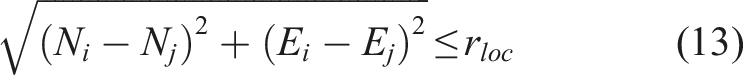
denote different data modes, for example, bathymetry and SSS. In our approach, the surveyed region is divided into geo-referenced patches of equal size, which we call • Contain multiple pixels to allow spatial patterns in the remote sensed data modes to be analysed • Be sufficiently large to absorb the impact of positional offsets that exist between data modes • Be smaller than the size of the habitats that are being characterised
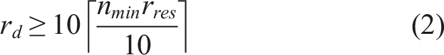
For the first point, although methods such as super-resolution can potentially be applied, we argue that this does not increase the basic information content. To fuse priors with different resolutions and channel depths, we first determine an appropriate patch size using the criteria below. The patch edge length r
d
(in metres) must lie in the range:


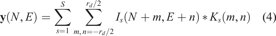
Each patch is discretised to match the feature learning network’s input layer, where we use zero-order sampling to match the resolution of each prior. This ensures the same geo-locations are indexed uniformly across each prior. A learnable 3 × 3 kernel, K
s
, is passed over each patch to fuse the different priors, where for priors with multiple channels (e.g., satellite imagery with RGB layers), each channel is weighted equally. To populate each patch, data from each mode s is fused as follows (Gunes and Piccardi, 2005):
3.2. Self-supervised feature learning
3.2.1. Location-guided autoencoder (LGA)
The LGA is a self-supervised method that extends the autoencoder (AE) to consider location information during feature learning. The AE is a learning architecture that consists of two neural networks, an encoder and a decoder. The former maps the input,

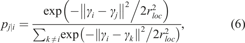
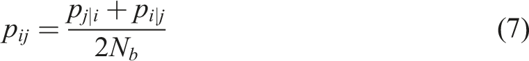
The LGA implements the proximity assumption by modifying the autoencoder loss function to consider location information (Yamada et al., 2021a). We first define p
ij
, which relates the distance between two inputs
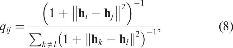
The affinity q
ij
is derived from
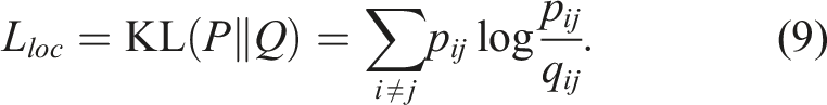

The LGA in this study uses the AlexNet (Hinton et al., 2012) as the encoder architecture, and its inverted counterpart is used as the decoder. Convolutional layers are transformed into transconvolutional layers, and max pooling layers are converted to max unpooling layers. The workflow of the LGA is illustrated in Figure 3(a). Self-supervised feature learning methods. Grey blocks indicate where parameters are optimised through the learning process. (a) The LGA introduces a geo-location-based loss term L
geo
to the standard autoencoder. The geo-location loss term prioritises patterns found between multimodal patches that are geographically close to each other by minimising the KL divergence between location and feature affinity matrices. This imposes a soft location constraint that prioritises features that recur in nearby location. The distance over which similarity is assumed is a parameter that can be tuned, where setting this to zero produces outputs that are identical to a standard autoencoder. (b) GeoCLR modifies SimCLR by selecting positive (i.e., similar) pairs from nearby locations 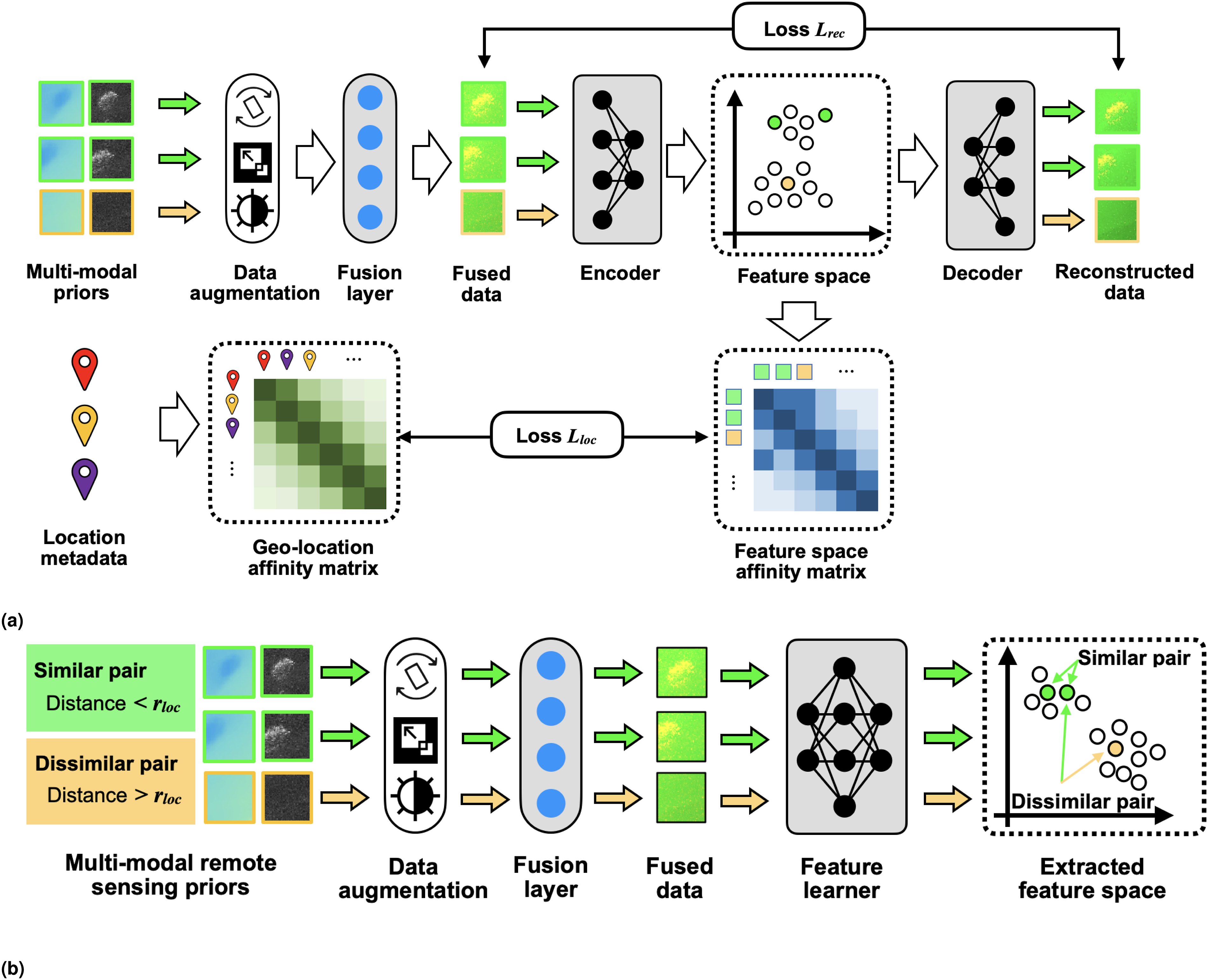
3.2.2. GeoCLR
GeoCLR implements a hard location constraint through contrastive feature learning. It extends SimCLR, which learns feature representations by maximising agreement in the feature space between differently augmented views generated from the same input
Features are extracted using a CNN encoder,
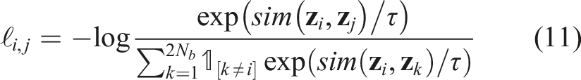
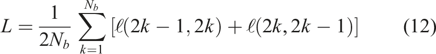
GeoCLR extends SimCLR and implements the proximity assumption by taking location information into account. Positive pairs are generated from distinct inputs [
Since the contrastive loss embeds positive pairs to nearby regions of the feature space, GeoCLR can be considered as a hard location constraint. As r
loc
increases, the positive pair
3.3. Visual class sampling
We use semi-supervised learning to train classifiers to predict visual classes over the remote sensed region. The training and test labels used for benchmarking are generated from visual images (Massot-Campos et al., 2023; Yamada et al., 2022) or by human experts. Since patches generated to discretise the remote sensed priors are typically larger than the footprint of AUV gathered imagery, those that have overlapping imagery are likely to contain multiple visual class labels for training and testing, where these are not guaranteed to be from a single class (Figure 1). Previous studies have used the most frequent label (He and Garcia, 2009; Leevy et al., 2018), or the most central label (Rao et al., 2017) as a definitive single label to use for training and testing purposes. However, this neglects the mixing of different habitat classes near boundaries. To address this, we assign multiple labels to each patch, accompanied by their respective proportions determined based on their frequencies within each patch (Shields et al., 2020), which actually becomes a probabilistic multi-class classification problem.
3.4. Habitat classification and prediction
Classifiers are trained to correlate patterns between learned feature spaces and class labels derived from a random subset of the visual images at each site. Their performance is determined based on the F1 scores against reference class labels derived from the remaining visual images that were not used for classifier training. We note the use of location-based regularisation does not affect the validity of the results since location information is only used during training, and not during testing and inference.
We investigate four well-established probabilistic and non-probabilistic classifiers to delineate the visual class boundaries in the feature space. Compared to non-probabilistic classifiers, probabilistic classifiers provide uncertainty estimates that indicate confidence in their predictions. Regions with high uncertainty may benefit from additional observations to improve correlation between patch features and their corresponding visual habitat classes, but it is also possible that the remote sensing priors do not contain the information required to characterise the environment.
The Support Vector Machine (SVM) is chosen to represent a non-probabilistic classifier due to its proven robustness and performance over a variety of geospatial classification tasks (Ojala et al., 2002). For probabilistic classifiers, we compare the performance of the Gaussian Process Classifier (GPC), Gaussian Process Regression (GPR) and a Bayesian Neural Network (BNN). Based on a preliminary optimisation study using the grid search method (Syarif et al., 2016), we deploy the radial basis function kernel in the SVM, the rational quadratic kernel in GPC and the Matern kernel in GPR, respectively, as these were found to provide the best performance for each classifier. The BNN classifier uses a fully connected neural network using three layers with 64, 32 and 8 nodes, respectively. Classification accuracy scores are determined using the visual image-derived class proportions in each test patch for all classifiers.
4. Experiments and analysis
4.1. Dataset description
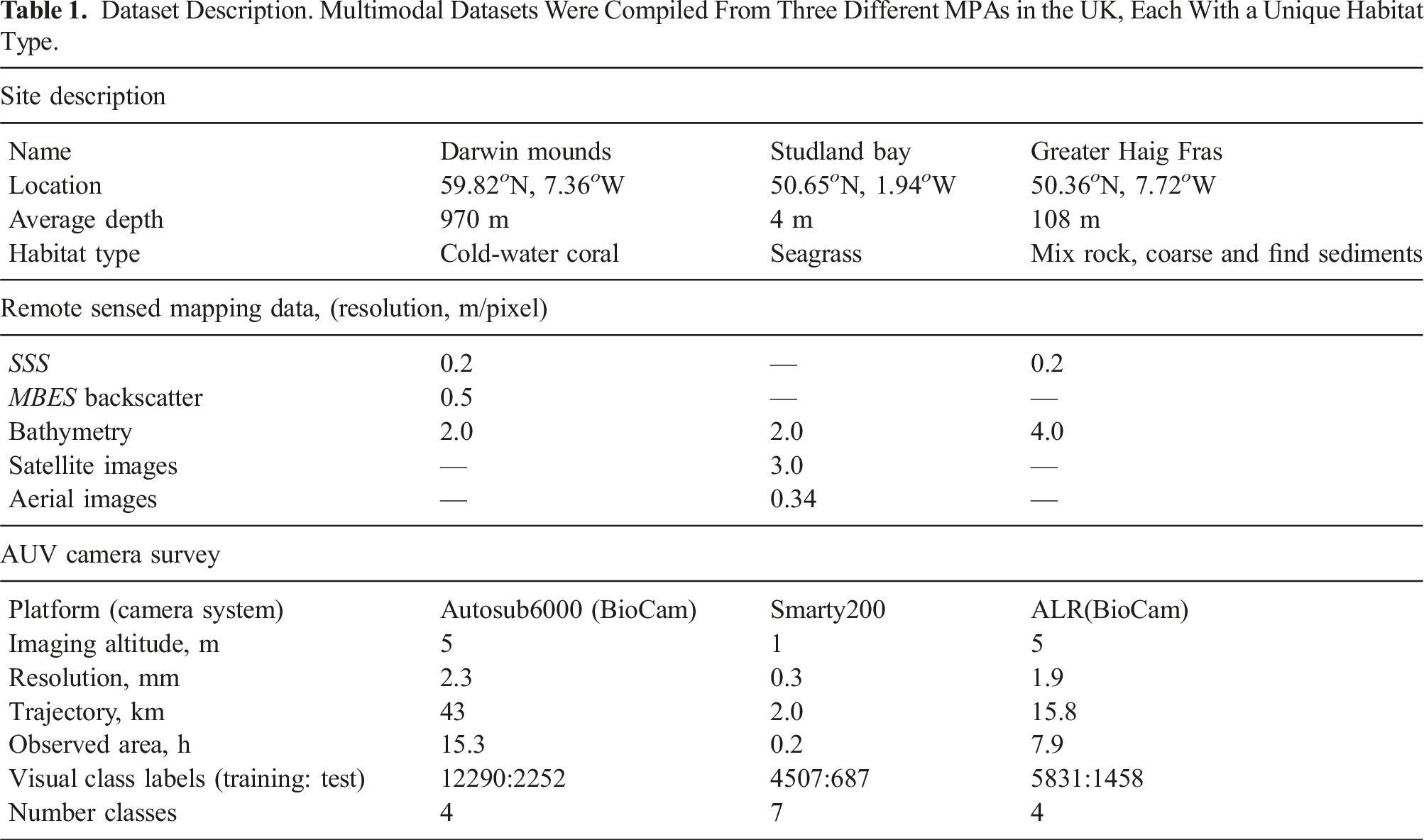
Experiments are carried out on multimodal datasets from three marine protected areas (MPAs) in the UK: Darwin Mounds (DM), Studland Bay (SB) and Greater Haig Fras (HF), as shown in Figure 4. The MPAs have different substrate and habitat types, and the datasets consist of various remote sensed mapping data and seafloor imagery taken by different AUVs (see Table 1). Further information about the data modes used in our comparative experiments can be found in the supplemental material. Locations of the three study sites are sketched as red boxes. Darwin Mounds (DM) is located 160 km northwest of Scotland, at seafloor depths between 710 and 1129 m. The site is characterised by cold-water-coral populated sediment Mounds and xenophyophores densely populated along mound tails (Huvenne et al., 2016). Studland Bay (SB) is located off the coast of Dorset, England, with depths up to 4 m. It is characterised by seagrass beds and long-snouted seahorses (Collins et al., 2010). Greater Haig Fras (HF) is located 95 km northwest of the Isles of Scilly at depths between 38 and 118 m. It is a mosaic habitat alternating between exposed bedrock, or rocky reef, and sediments (Benoist et al., 2019). The images show examples of each visual class, and the pie charts indicate the relative class proportions observed during AUV camera surveys. Dataset Description. Multimodal Datasets Were Compiled From Three Different MPAs in the UK, Each With a Unique Habitat Type.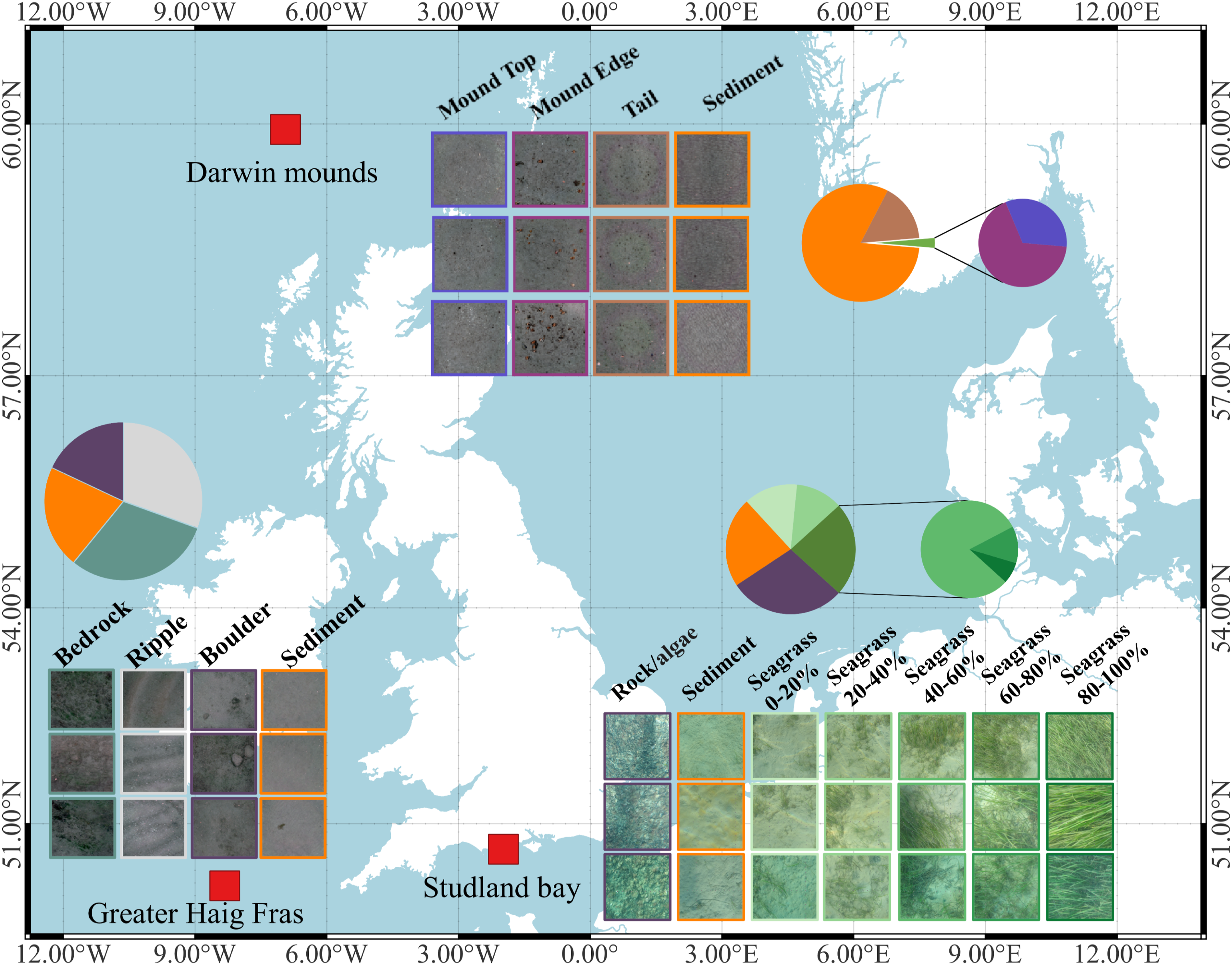
4.1.1. Darwin Mounds
Darwin Mounds is a Special Area of Conservation (SAC) located 160 km northwest of Cape Wrath, Scotland. The area is characterised by sandy mounds that support cold-water coral colonies at a depth of approximately 1000 m (Huvenne et al., 2016). A visual imaging survey was conducted in 2019, using the National Oceanography Centre’s Autosub6000 which was equipped with the University of Southampton’s BioCam high altitude 3D imaging system to survey the region from 5 m altitude. Four visual classes exist in the image dataset: Sediment (81%), (Mound) Tail (16%), Mound Edge (2%) and Mound Top (1%), where Figure 4 shows class exemplary images and relative proportions observed by the AUV. Classification of visual images was performed using semi-supervised learning following the method described in Yamada et al. (2023). Validation against 100 expert human-labelled reference images from each class gave an F1 score of 84%, showing strong performance despite the significant class imbalance. The predicted visual class labels are used as the reference for training and testing in this paper. SSS (Huvenne et al., 2016) and MBES (Wynn et al., 2014) survey data from 2011 were used as remote sensed priors, where physical changes in the environment can be considered negligible relative to the remote sensing resolution (0.2 m) considering the slow growth rate of the Mounds (<3 mm/year (Victorero et al., 2016)) and protected status preventing any trawl activity in this region.
4.1.2. Studland Bay
Studland Bay is a Marine Conservation Zone (MCZ) located on the Dorset coast. The water depth is <4 m and extensive seagrass meadows are visible in satellite and aerial images (Massot-Campos et al., 2023). The seagrass meadows provide a habitat and breeding ground for various fish species including seahorses. A survey was carried out in September 2022 using the University of Southampton’s Smarty200 AUV, with images taken from a low altitude of 1 m. The AUV took 5634 images that were classified following the method described in Yamada et al. (2023) into seven classes, five of which are different percentage covers of seagrass: Rock/algae (29%), Sediment (22%), Seagrass 0%–20% (13%), Seagrass 20%–40% (12%), Seagrass 40%–60%, (19%) Seagrass 60%–80% (3%), and Seagrass 80%–100% (2%), respectively. Figure 4 shows imagery and class proportions, which are significantly imbalanced. Validation against 100 expert human-labelled reference images from each class gave an F1 score of 60%, where most confusion occurred between adjacent seagrass cover percentages. The exemplary images illustrate the visual similarity across class boundaries, where discretizing naturally continuous variations is challenging for both human experts and algorithms. This paper uses the predicted visual class labels as the reference for training and testing. SI data was taken from Sentinal-2 on the same date as the AUV survey, and AI was obtained from Google (2021) with a data collection date in July 2021. The depth data was obtained from the United Kingdom Hydrographic Office, with a data collection date of 2012. Although robust evidence for temporal trends in seagrass meadow cover at Studland Bay does not exist, reported changes are
4.1.3. Greater Haig Fras
The Greater Haig Fras (HF) region is a SAC mosaic habitat (depth from 38 to 100 m), characterised by rocky reefs alternating with sediments. The AUV camera survey was done in July 2022 using the National Oceanography Centre’s Autosub Long Range (ALR), which was equipped with the University of Southampton’s BioCam camera system. The image dataset used here consists of 7289 images that were classified by human experts into four classes: Sediment (31%), Bedrock (30%), Ripple (21%) and Boulder (18%), showing relative balanced between classes. SSS data was taken by the Autosub6000 AUVs of NOC (Zelada Leon et al., 2020) in 2015 using Edgetech sidescan sonar and the bathymetry data was collected in 2014 by the United Kingdom Hydrographic Office. Considering the substrate types in the surveyed region, temporal variations can be considered negligible in this region.
4.2. Experimental setup
The patch size used in this study has r
d
= 10 m, which is the smallest patch size that satisfies the criteria in equations (1)–(3) for our datasets. The patch window was shifted by an interval of 5 m and all patches were used for feature learning. Two sets of experiments were carried out to investigate the following aspects of performance: • Effectiveness of multimodal feature learning with location regularisation for habitat classification • Robustness to distance hyperparameter tuning • Sensitivity to data inconsistencies when combining multimodal priors
For the LGA and AE, AlexNet was used as the encoder network where the latent representation dimension was set to 16. The network was trained for 100 epochs with a learning rate of 1.0 × 10⁻⁵, λ = 1.0 × 10³ and the weight decay was set to 1.0 × 10⁻⁵, with a minibatch size of N d = 128 following the recommendations of Yamada et al. (2023). For the LGA, the distance parameter was set to r loc = 8 m to apply the soft proximity assumption to all neighbouring patches.
Experiments with GeoCLR and SimCLR used ResNet18 as the underlying architecture. The latent representation
AE-LGA and SimCLR-GeoCLR network training epochs were fixed to 100 and 800, respectively. Network training took 7 h and 30 h, respectively, on a NVIDIA TITAN RTX 24 GB GPU. Computing the distance metrics from location metadata for LGA and GeoCLR took less than a minute, which is negligible compared to the total network training time.
Experiments were performed using both single mode and multimodal priors, where multimodal experiments combine remote sensed backscatter (SSS or MBES) or imagery (SI or AI), with bathymetric data (depth or relative depth (RD)). RD was calculated using equation (14):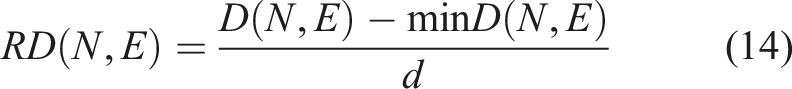
To investigate the sensitivity of each method to the distance hyperparameter, we selected the remote sensed priors that give the best multimodal inference results and investigated the sensitivity of the results to tuning of the location regularisation (i.e., distance parameter r loc ). The value of r loc was varied between 0, 8, 15, 22, 44, 66, 100 m for both the LGA and GeoCLR, where r loc = 0 corresponds to the AE and SimCLR, respectively. The final set of experiments investigates the robustness of the method to data inconsistencies between the remote sensed priors by introducing 2.5, 5, 7.5 and 10 m positional offsets between each mode being combined.
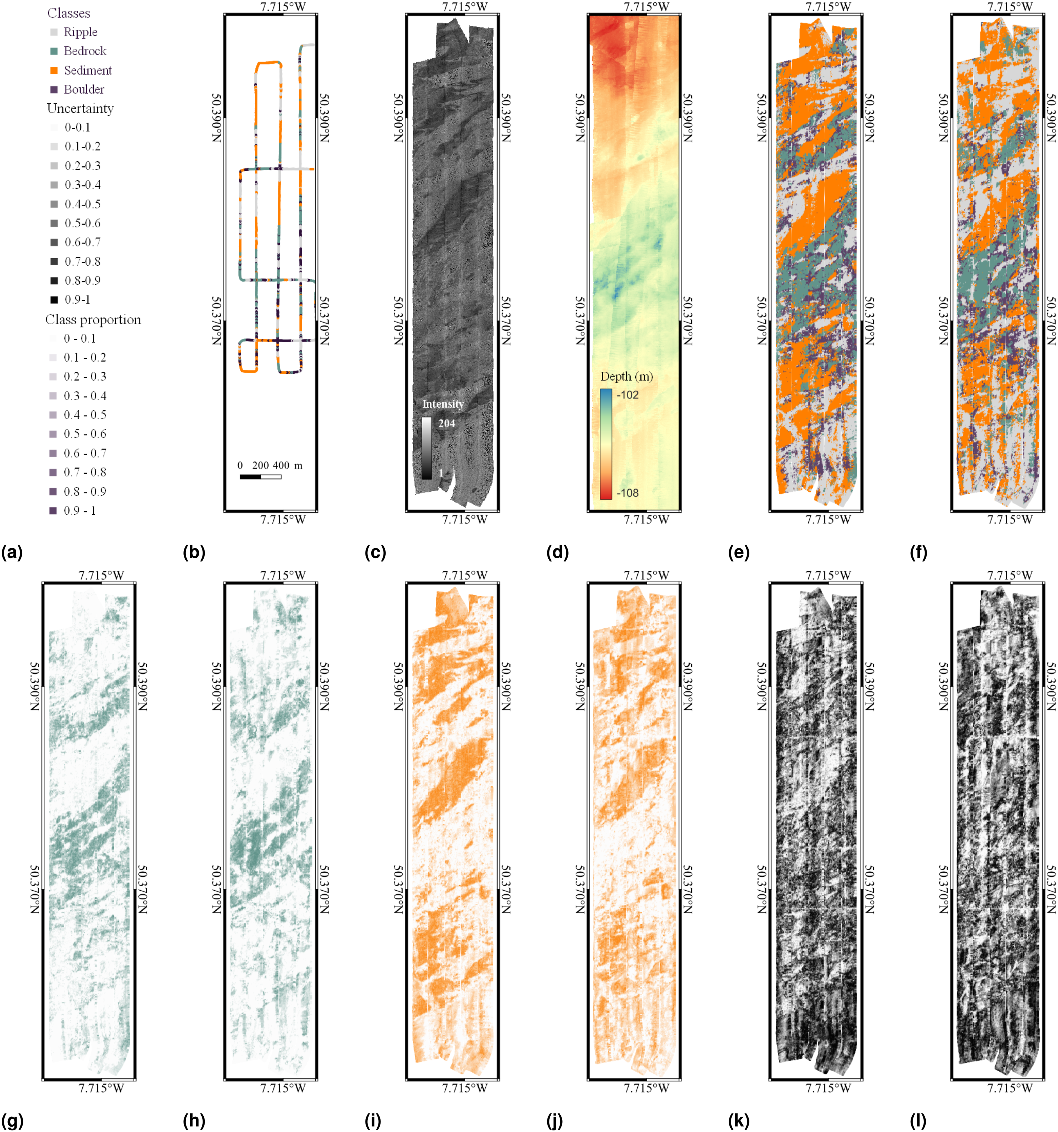
The macro F1 score, averaging precision for each predicted class and recall for each labelled class (Grandini et al., 2020), is used to evaluate multi-class prediction performance. Specifically, we compute the average class proportion error as the differences between the predicted and labelled class proportions for each pair of classes over the testing dataset. Based on this, a confusion matrix of accuracy can be constructed, enabling the calculation of the macro F1 score for probabilistic multi-class classification. For visualisation purposes, the habitat maps in Figures 7–9(e) and (f) assign the class with the highest predicted proportion per patch. Figures 7–9(g)–(j) show the proportion of an individual class within each patch.
4.3. Multimodal feature learning and classifier performance
Results comparing the performance of the different feature learning and classification methods are summarised in Figure 5, while full tables of results can be found in the supplemental material. The results show that early fused multimodal data consistently outperforms the use of a single mode, and that location regularisation improves the performance of both the AE based and contrastive feature learning models. The hard location constraint of GeoCLR outperforms the soft location constraint in LGA, with GeoCLR achieving 16.7% higher average F1 score overall conditions. The best results for each dataset are achieved by GeoCLR using multimodal data, reaching 79.0%, 56.8% and 83.0% for DM, SB and HF, respectively. The lower F1 score for the SB dataset is attributed to this being a harder classification problem, with a large number of visual classes that have a similar appearance (i.e., seagrass with varying percentage cover). F1 scores of habitat classification using AE, LGA, SimCLR and GeoCLR as feature extraction methods. The results reveal that LGA and GeoCLR are generally better than AE and SimCLR, respectively. In addition, multimodalities also enhance the classification performance.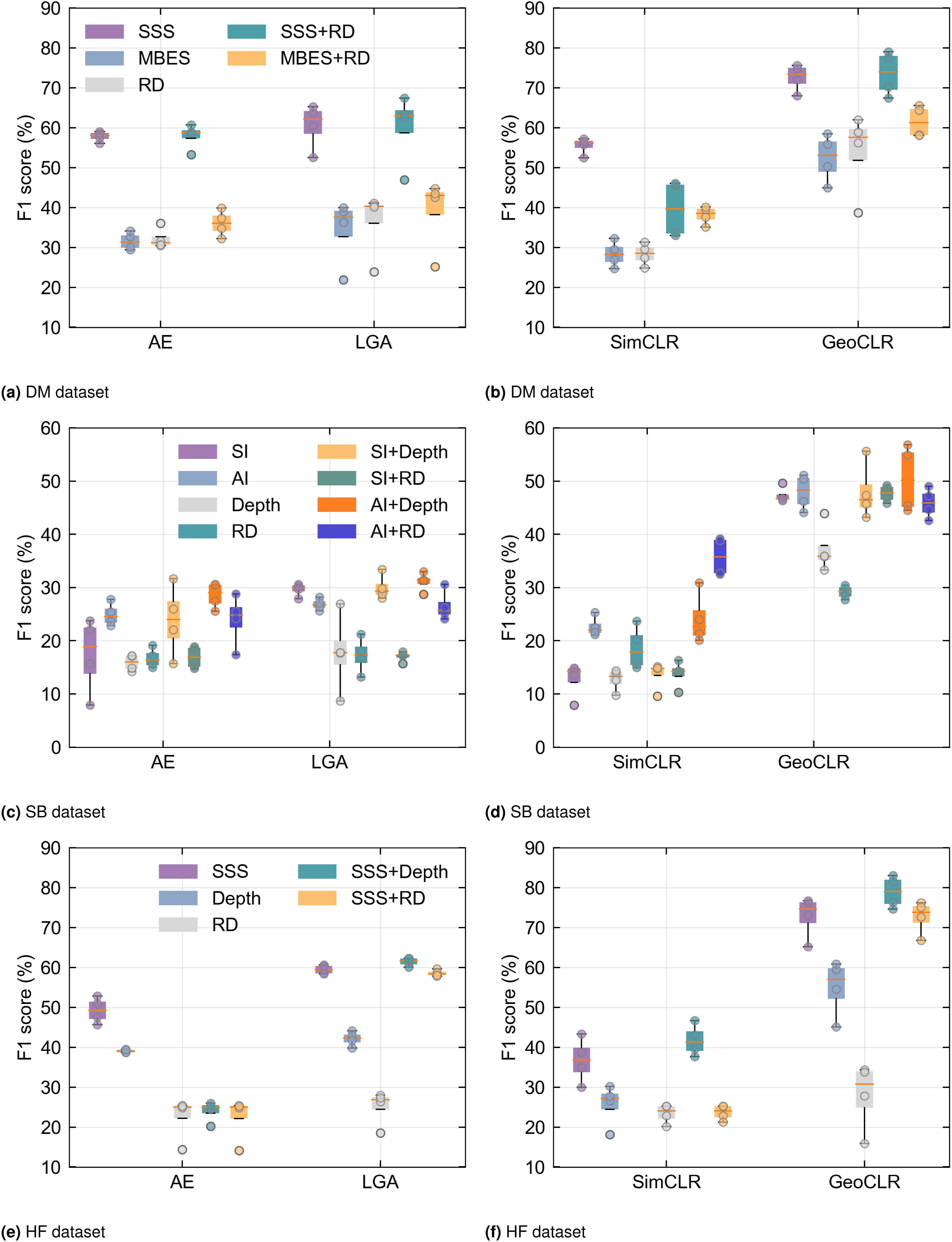
For the DM dataset, combining SSS + RD achieves an F1 score of 79.0%, improving performance over the best-performing single mode SSS by 3.4%. Similar improvements are seen for SB, with AI + Depth achieving 56.8%, improving the best-performing single mode AI by 6.4%, and for HF SSS + Depth achieved 83.0%, outperforming the best single mode SSS by 6%. In general, GeoCLR improves F1 scores when combining modes, increasing the F1 score by an average of 5.27% over the best-performing individual mode it combines, demonstrating its ability to take advantage of multimodal patterns in early fused data. However, improvement is not guaranteed in cases where there is a large discrepancy in the information content of the layers being combined. For example, RD performs poorly for the SB and HF datasets (F1 scores <30% across all conditions), and when combined with higher-performing single modes, the combined F1 score falls short of the single mode score in some of the cases. However, even in these scenarios, the F1 score is significantly higher than the average of the modes being combined (on average 11.9% higher), indicating that rather than just naively merging information, feature learning actively rejects poor information content. This property is also demonstrated by LGA, which improves over the average of combined modes by 4.7%. An interesting results for the DM dataset is that although combining MBES + RD improves performance (65.6%) over each individual mode (58.5% and 62.0%), the overall performance is still significantly below SSS + RD (79.0%). The backscatter measurements of MBES originate from the same acoustic pulses used to determine RD (i.e., same sensor and signal, but using different processing). Therefore, these datasets have perfect alignment. On the other hand SSS backscatter data has an average positional offset of 12.0 m relative to RD due to localisation uncertainty and different measurement physics causing geometric distortions between the dataset (discussed in the supplemental material). Despite this the higher quality of acoustic backscatter information in the SSS outweighs any negative impacts of these spatial inconsistencies when combining the layers. A more detailed investigation into the effects of spatial inconsistencies will be discussed in the robustness analysis section.
Figure 6 summarises the performance of each classifier across all feature learners. Probabilistic classifiers (GPC, GPR, BNN) marginally outperform the non-probabilistic classifier (SVM) by 3.4% for equivalent feature and dataset conditions. The overall performance is less dependent on classifier choice than feature learners. However, probabilistic classifiers can provide uncertainty estimates for predictions, which may be advantageous in scenarios such as path planning where a larger proportion of observations could be gathered from such areas to improve the prediction certainty. Average performance of classifiers in studied cases for each dataset regardless feature learners. There is no significant difference between classifiers in terms of F1 score.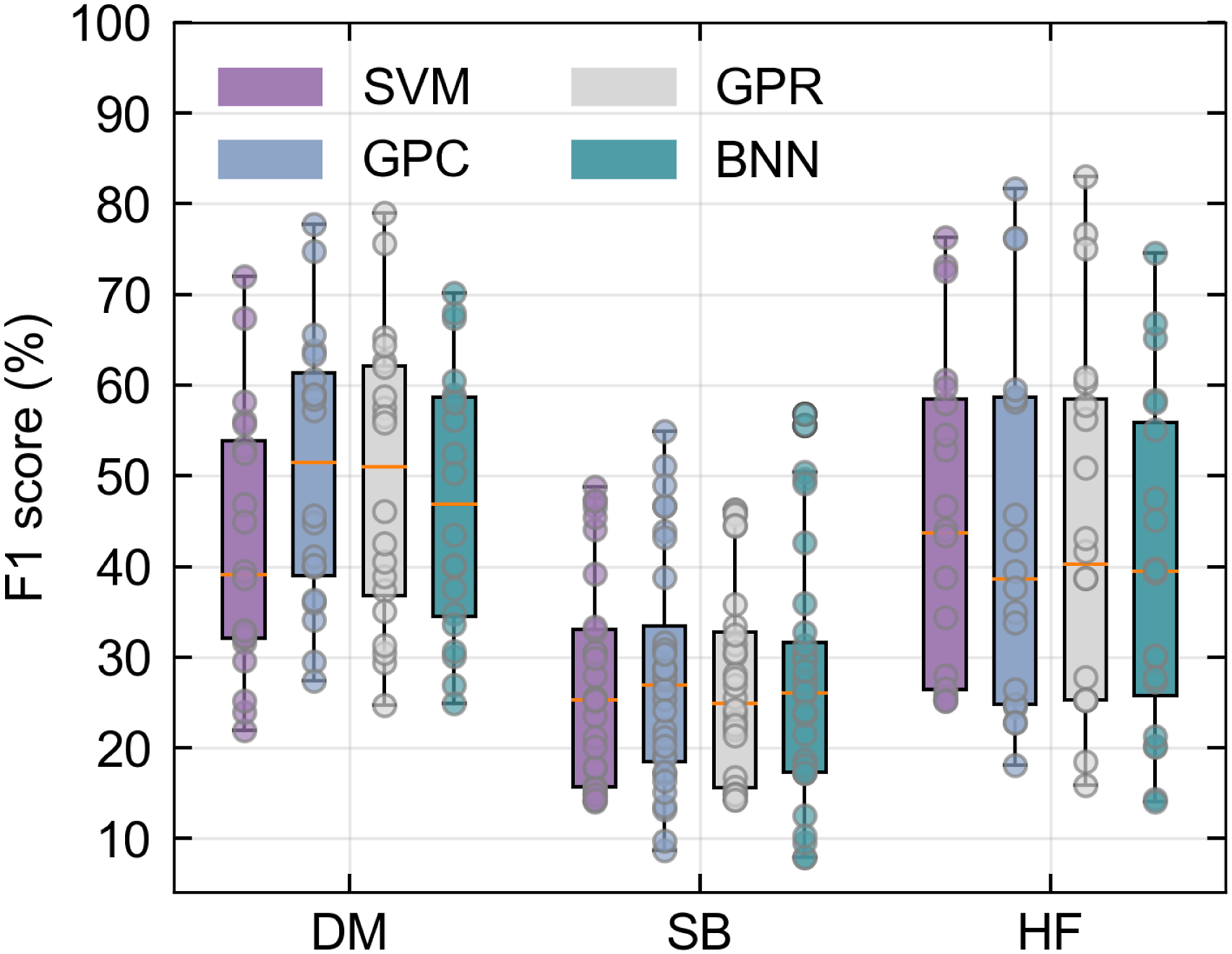
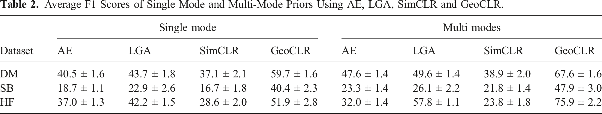
4.4. Importance of location metadata
Average F1 Scores of Single Mode and Multi-Mode Priors Using AE, LGA, SimCLR and GeoCLR.
4.5. Habitat class prediction and class uncertainty
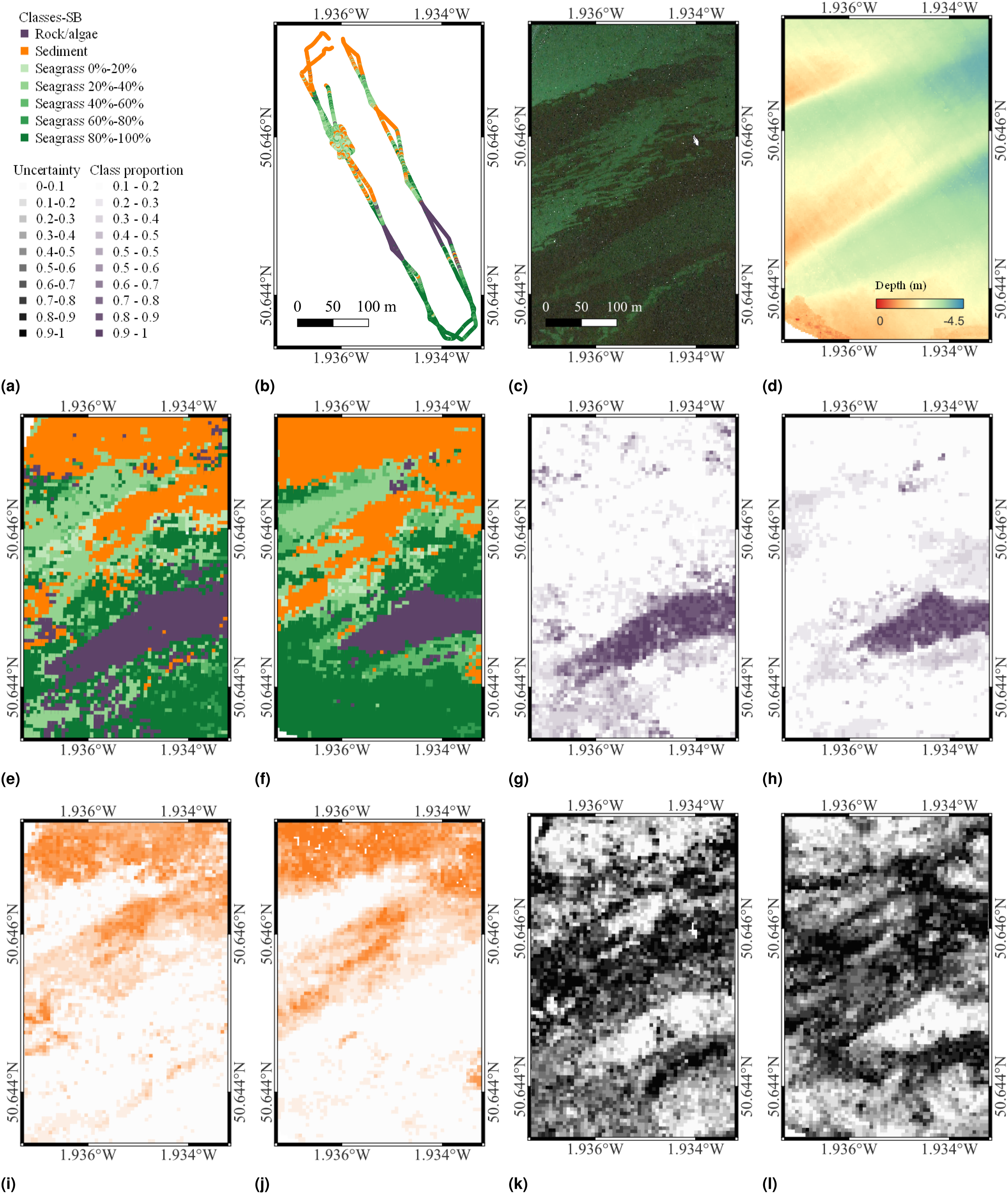
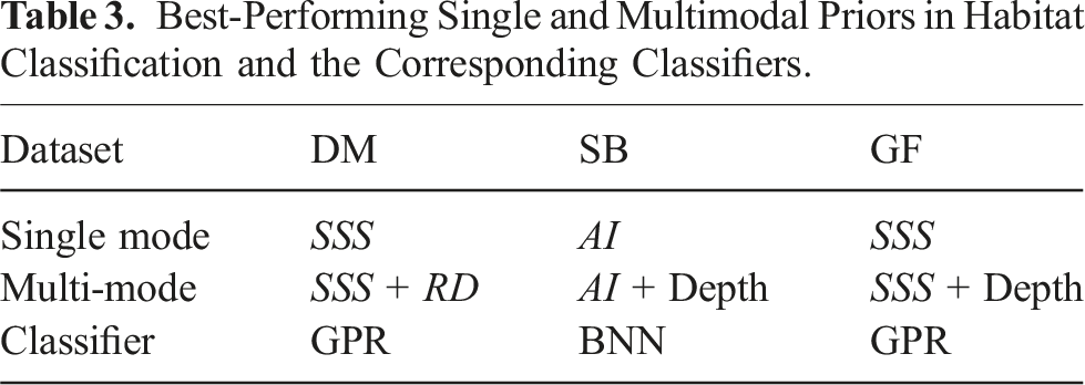
Figures 7–9 show the best performing single and multimodal remote sensing priors, visual class training inputs and classification results for the DM, SB and HF datasets, respectively. The predicted visual class distribution for single and multimodal scenarios corresponds to the best-performing feature learner and classifier pairing (see Table 3). In Figures 7 and 9 for the DM and HF datasets, panels (e) and (f) show the class with the highest predicted proportion within each patch, and panels (k) and (l) present uncertainty maps given by the classifier, which reflect the confidence of the classifier to predictions. Figure 8 also shows the same information for the SB dataset. Habitat classification results for the DM dataset, showing (a) the figure legend; (b) the reference class distribution derived from visual images; (c) SSS; (d) Depth; (e) and (f) are habitat classification results using a single mode data SSS and multimodal data SSS + RD; (g) and (h) are example class proportion maps of Mound edge inferred by GPR classifiers using single mode and multimodal data, respectively; (i) and (j) are example class proportion maps of Mound top. It can be seen that class boundaries are clearer when using multimodal priors (see boxes in red); (k) and (l) show uncertainties given by GPR classifier. Habitat classification results for the SB dataset, showing (a) the figure legend; (b) the reference class distribution derived from visual images; (c) and (d) are the aerial images (AI) and Depth priors; (e) and (f) are classification maps inferred from AI and AI + Depth; (g) and (h) are example class proportion maps of class Rock/algae inferred from single mode and multimodal priors; (i) and (j) are example class proportion maps of Sediment inferred from single model and multimodal priors. (k) and (l) present the uncertainties given by the BNN classifier. Habitat classification results for the Greater Haig Fras, showing (a) the figure legend; (b) the used reference class distribution derived from visual images (full visual image dataset class distribution could be seen in supplemental materials); (c) and (d) are SSS and Depth data; (e) and (f) depict the habitat classification results derived from the single mode data SSS and multimodal data SSS + Depth, respectively; (g) and (h) are example class proportion maps of Bedrock inferred from single mode and multimodal priors; (i) and (j) are example class proportion maps of Sediment inferred from single mode and multimodal priors; (k) and (l) present the uncertainty in given by GPR classifiers. Best-Performing Single and Multimodal Priors in Habitat Classification and the Corresponding Classifiers.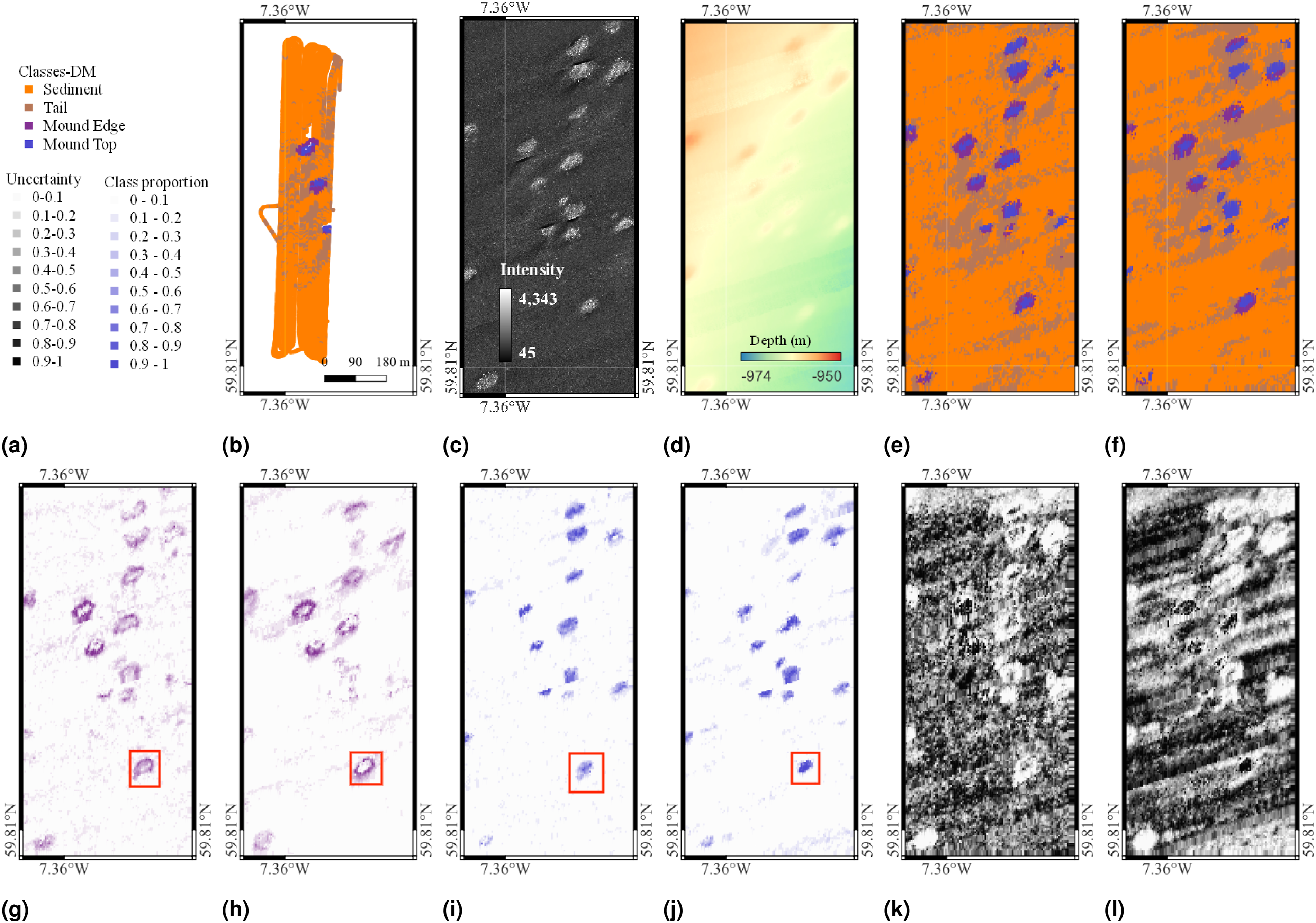
In the DM dataset, Figure 7(f), corresponding to multimodal inputs (SSS + RD), diagonal strips exist in classification maps, which are caused by the offsets seen between adjacent passes of the AUV when gathering bathymetry data. Although these are artefacts, the overall F1 achieved using multimodal data is higher than the best performing single mode input SSS (see Figure 7(e)), showing robustness to common practical issues relating to input data quality. The predicted proportion and distribution of Mound Top, where the majority of cold-water corals are found are relatively similar between the single and multi-mode scenarios in Figure 7(e) and (f), respectively.
The SB dataset results show a similar overall distribution pattern between Figure 8(f) for multimodal (AI + Depth) classification and Figure 8(e) for the best single mode (AI). The AI image has a boat visible in the data, where this region was masked during training and testing and adopted the most frequent predicted class of its nearest neighbours. Although the overall distribution patterns are similar, the Rock/algae in the bottom left predicted by the single mode Figure 8(e) is not predicted in the multimodal case in Figure 8(f), where the predictive uncertainty is also higher in this region compared to the single mode case. The multimodal individual class proportions show a transition from the Rock/algae class and the Seagrass 80%–100% class in this region.
For the HF dataset, we also see similar overall distribution patterns between the single mode (SSS) and multimodal (SSS + RD) inputs. However, Figure 9(l) shows less uncertainties in the Sediment class for the multimodal input compared to the single mode classification shown in Figure 9(k).
Overall, inconsistencies among multiple priors tend to increase predicted class and uncertainty. This is reflected by reduced F1 scores in these areas which is the expected behaviour and illustrates that the classifiers demonstrated in this work provide useful predictions of uncertainty in their class predictions. A detailed discussion of proportion maps for other classes is provided in the supplemental material.
4.6. Sensitivity to distance parameters
The parameter r loc in both LGA and GeoCLR determines the distance over which the proximity assumption is applied during self-supervised feature learning. In order to understand its impact, a sensitivity analysis is conducted using the best priors and classifiers for each dataset (i.e., conditions in Table 3).
The results across the three datasets over an order of magnitude difference in the value of r
loc
are shown in Figure 10. Compared to LGA, GeoCLR is more sensitive to the distance parameter, which is an expected outcome given the hard constraint implemented by contrastive learning. GeoCLR achieves the best results when location metadata is set so that only neighbouring patches are used as positive pairings, where the improvement deteriorates with the increasing r
loc
, which can be explained as positive pairings being forced from regions of the data that are apart and so more likely to be of different visual classes. The results for single and multimodal inputs follow a similar trend with increasing r
loc
from 8 to 100 m. However, even with over an order of magnitude of the r
loc
value, GeoCLR outperforms the equivalent SimCLR that does not implement the location regularisation. The performance of habitat classification varying with the distance hyperparameter r
loc
for the best performing multimodal data and classifier for each MPA. The top row shows results for the LGA for (a) DM, (b) SB and (c) HF datasets. The bottom row shows results for the GeoCLR for (d) DM, (e) SB and (f) HF datasets. For all cases, performance improvements are achieved compared to equivalent feature learning without the proximity assumption (i.e., AE and SimCLR) for all tested distance parameters, which span an order of magnitude in value. The LGA is less sensitive to variations in the distance hyperparameter, with 7.5% deviation in F1 from its optimal performance, though the overall gain in performance from using distance with the soft constraint is less than for GeoCLR. GeoCLR is more sensitive, with 14.6% deviation in F1 from its optimal performance. The different behaviours highlight the inherent properties of the soft and hard location constraints implementation by the LGA and GeoCLR, respectively.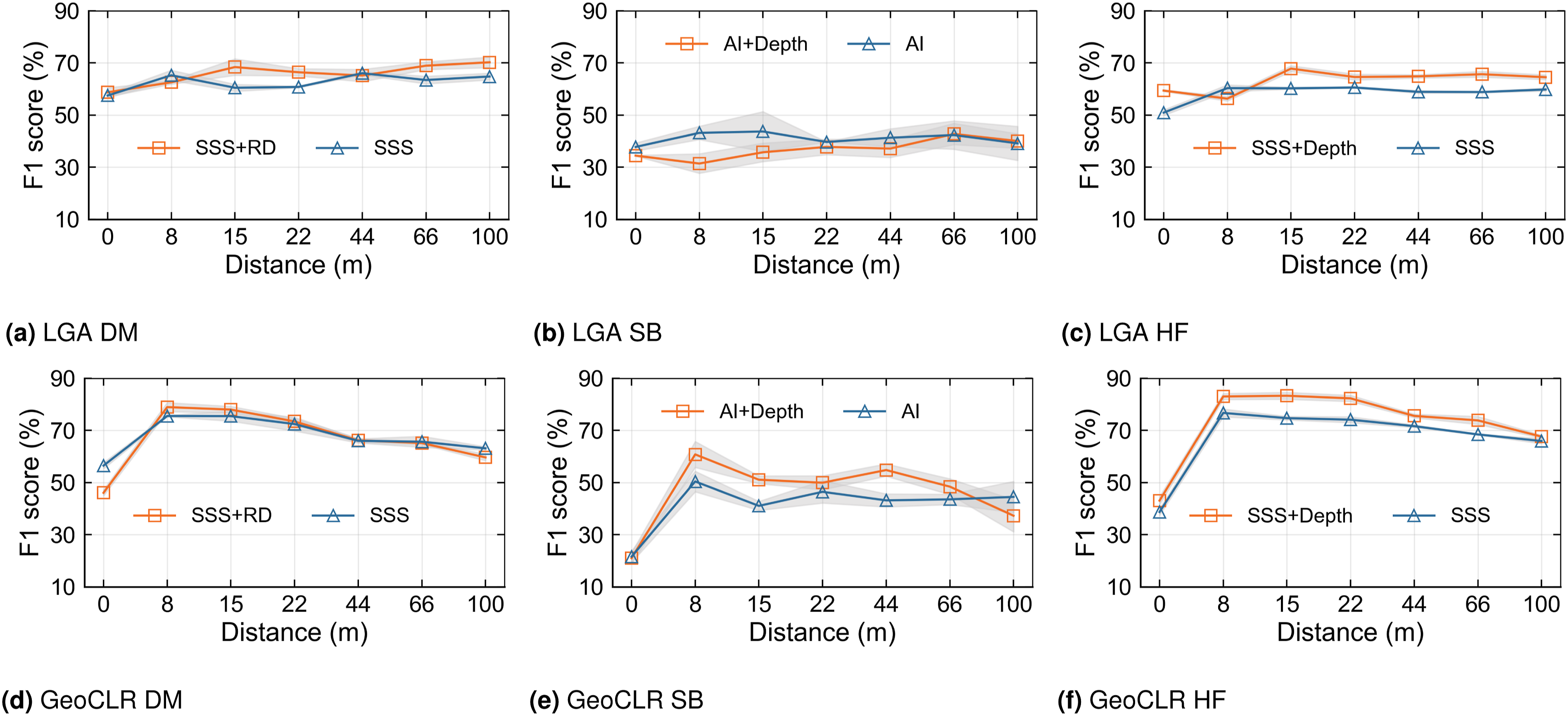
The LGA is less sensitivity to variations in r loc over the same range. This is expected since the soft constraint implemented via the modified loss function prioritises features of patches in geographically closer regions in a smooth manner, where the reconstruction loss term means that patches that do not have similar appearances in the first place can remain far apart in the feature space, minimising the risk of overfitting the proximity constraint. The results for single and multimodal inputs show a less obvious trend with increasing r loc , where the performance gains over AE are generally smaller, and are maintained over the entire range of distance parameters tested.
4.7. Robustness analysis
Multimodal data has inherent positional offsets between individual data modes. Information about the actual positional offset magnitude and direction for multimodal data used in this study is given in the supplemental material (Table A1). Manually co-registered points between the data layers have large variability in their offset magnitude and direction, which can be explained as due to geometric distortions that are known to occur in some measurements modes, for examples, SSS. To investigate the robustness of our models to these practical aspects, we introduced artificial offsets in various directions (45°, 135°, 225° and 315°), with magnitudes of 2.5 m, 5 m, 7.5 m and 10 m, respectively, based on representative positional errors of 10 m in subsea mapping (Paull et al., 2014). No significant correlation was found between the directions of the true and artificial offset directions, and so here we present only bulk statistics for the different offset distance magnitudes.
The choice of patch size can influence the training and robustness of the model. Large patches can degrade performance, in particular around habitat transition areas where seafloor characteristics can change over small spatial scales causing nearby patches to have different characteristics. Conversely, smaller patches risk omitting significant patterns critical to classification. Therefore, determining an appropriate patch size requires careful consideration of prior resolution and the scale of habitats, as guided by equations (1)–(3).
The impact of introducing different artificial positional offsets on the performance of multimodal feature learning varies across the three datasets. As a reference, the results in Figure 11 include conditions that do not implement location regularisation during feature learning (i.e., r
loc
= 0 corresponding to AE and SimCLR), and compare optimally tuned conditions r
loc
= 8 m to r
loc
= 100 m. Larger positional offsets gradually reduce the performance of multimodal inference but the overall reduction in performance remains Habitat classification performance with different positional offsets for r
loc
values of 0, 8 and 100 m. LGA and GeoCLR with r
loc
= 0 correspond to AE and SimCLR, respectively. Based on the sensitivity research of r
loc
as shown in Figure 10, the best-tuned r
loc
is around 8 m. The conditions where r
loc
= 100 are taken as comparative experiments. All methods show reduced performance as positional offsets are introduced, but the benefit of using location metadata during feature learning are maintained for both optimised and unoptimised hyperparameter values.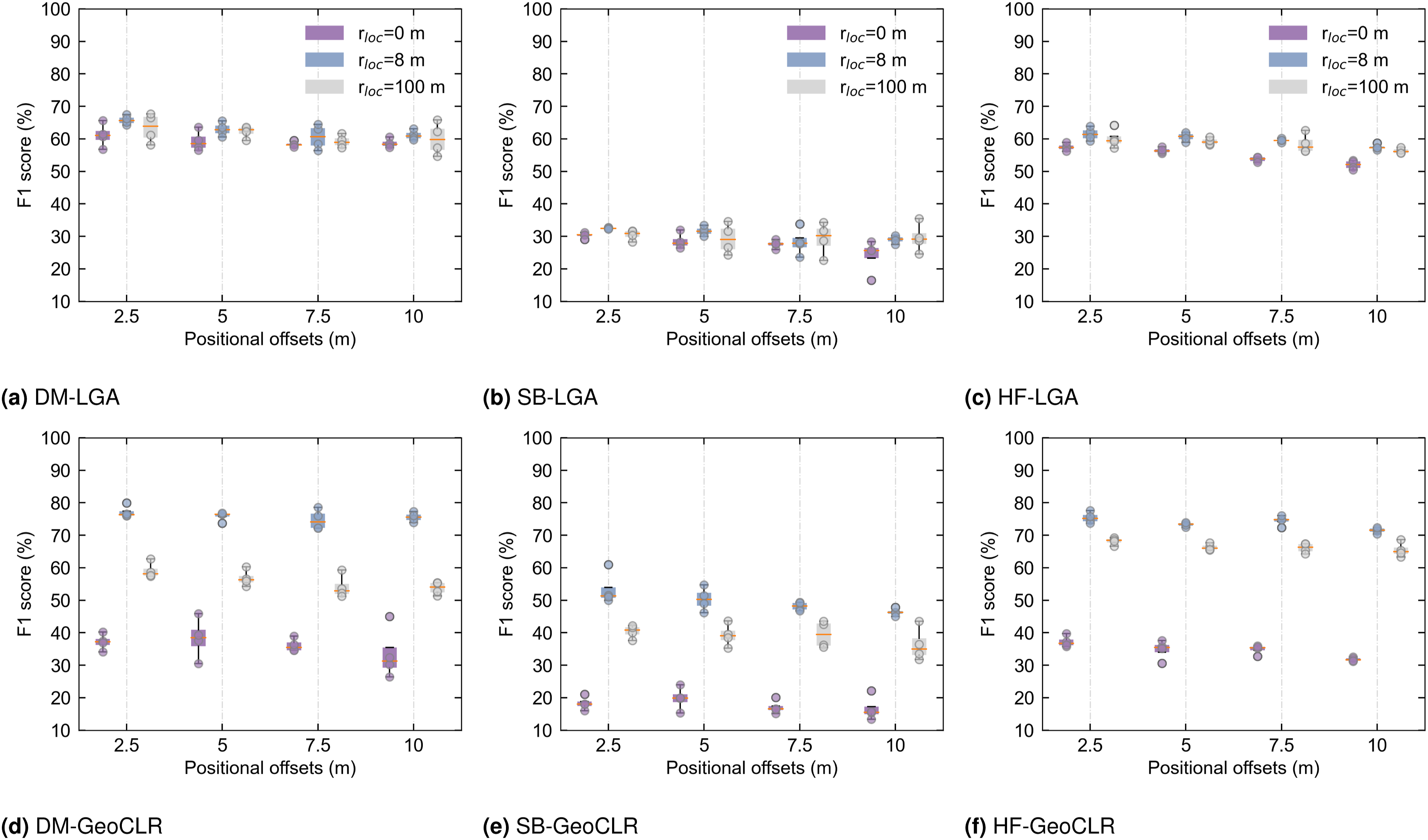
Based on the results, we can conclude that LGA is less sensitive to the distance parameter rloc and more robust to positional offsets compared to GeoCLR, which implements a harder distance constraint in contrastive learning. However, it is important to note that GeoCLR remains the most effective feature learning method, outperforming AE, LGA and SimCLR in all the investigated scenarios.
5. Conclusion
The method proposed in this study enhances marine perception by integrating multiple layers of prior data and observations. This can potentially be used to develop informative or adaptive path planning strategies during AUV surveys. Our investigation shows that incorporating location metadata improves the ability of self-supervised feature learners to take advantage of early fused multimodal mapping data, robustness to hyperparameter tuning and positional offsets in the remote sensed data. Experiments carried out on datasets from three different MPAs show that: • Incorporating location metadata enhances the quality of extracted features, where an average improvement of 18.3% across three datasets was achieved compared to features extracted with no location metadata when using a single modality. We demonstrate that a hard location constraint, that is, GeoCLR, results in a larger improvement (28.8%) compared to a softer location constraint, that is, LGA, (improvement of 7.7%) when the distance parameter is optimally tuned. LGA is less sensitive to distance parameter tuning than GeoCLR, where the use of location metadata improves performance over equivalent feature learners and conditions that do not use location metadata for all distance parameters (r
loc
= 8, 15, 22, 44, 66 and 100 m) investigated in this study. Although LGA is less sensitive to the distance parameter, GeoCLR exhibits a higher overall performance across the experiments in this work, with a 16.8% improvement in the F1 score compared to the LGA under equivalent conditions. • Early fused multiple remote sensed modalities increase classification performance over the best single mode when using self-supervised feature learners that incorporate location information and further boost habitat classification performance, showing an average increase of up to 5.1% across three datasets compared to using a single modality. Improvement of 3.3% and 6.8% were achieved for GeoCLR and LGA, respectively. The method also demonstrates robustness when combining data modes with poor information content, achieving improvements of 11.9% and 4.7% over the average F1 of the individual mode being combined when using GeoCLR and the LGA, respectively. The improved performance can be attributed to the use of location metadata during feature learning as equivalent autoencoders and contrastive learning with SimCLR did not achieve consistent improvement when using multimodal inputs. The use of location metadata also showed robustness of multimodal performance to positional inconsistencies between multimodal inputs, with performance decrease remaining • Investigations of different classifiers to delineate feature spaces according to visual class boundaries showed that probabilistic classifiers performed marginally better than the non-probabilistic classifier for the patch size chosen in this work, resulting in an improved predicted visual class F1 score of 3.4%. This is because multiple visual class labels exist for each patch due to the lower resolution of remote sensed priors compared to the in situ observations. However, no single classifier performed best across all datasets and feature learners, highlighting the importance of empirical optimisation. The GPR and BNN probabilistic classifiers that achieved the highest F1 scores in this study have the advantage of being able to predict class proportions and indicate inter-class confusion, which can be useful for interpretation or path planning.
Our experiments found that GeoCLR consistently outperformed SimCLR and LGA for feature extraction. Combining multimodal priors generally improved performance. Although the choice of classifier does not significantly impact F1-scores, using probabilistic approaches like GPC, GPR and BNN can predict class proportions and their associated uncertainties. This is valuable for addressing the varying extents of camera observations and the size of remote sensing patches. The uncertainty estimates provide valuable information for downstream applications.
Other key considerations include the patch size and the distance metric over which to apply the proximity assumption during feature learning. Patch sizes need to be large enough to contain a sufficient number of remote sensing pixels to capture characteristic patterns, while remaining smaller than the minimum size of the habitat being characterised. Within these constraints, although larger patch sizes contain more information, this does not necessarily improve performance as they have a higher chance of violating the proximity assumption used during feature learning. The distance metric should be smaller than the minimum size of the habitat being characterised, with GeoCLR showing gradual degradation in performance when the distance metric exceeds the length scale of habitats. However, it is more important to ensure that the distance metric is large enough for neighbouring patches to be available as similar in order to taking advantage of location-based regularisation during feature learning.
Supplemental Material
Supplemental Material - Self-supervised learning with multimodal remote sensed maps for seafloor visual class inference
Supplemental Material for Self-supervised learning with multimodal remote sensed maps for seafloor visual class inference by Cailei Liang, Jose Cappelletto, Miquel Massot-Campos, Adrian Bodenmann, Veerle AI Huvenne, Catherine Wardell, Brian J Bett, Darryl Newborough and Blair Thornton in The International Journal of Robotics Research
Footnotes
Acknowledgements
Datasets used were collected during NERC CLASS (NE/R015953/1) and Oceanids BioCam cruises of the RRS Discovery (NE/P020887/1 and NE/P020739/1) with the support of the NOC MARS team. Trials in Studland Bay were supported by the SMMI, Dorset Council, the National Trust and the Seahorse Trust. We acknowledge the United Kingdom Hydrographic Office for the bathymetry data of Studland Bay and Greater Haig Fras datasets. Copernicus Sentinel data 2019, processed by ESA and Google Earth (GE) were used for satellite and aerial imagery of Studland Bay.
Declaration of conflicting interests
The authors declared no potential conflicts of interest with respect to the research, authorship, and/or publication of this article.
Funding
The authors disclosed receipt of the following financial support for the research, authorship, and/or publication of this article: This research was supported in part by the Kakenhi Grant Aid B (22H01695) of the Japan Society for the Promotion of Science. Cailei Liang is funded by the China Scholarship Council.
Supplemental Material
Supplemental material for this article is available online.
References
Supplementary Material
Please find the following supplemental material available below.
For Open Access articles published under a Creative Commons License, all supplemental material carries the same license as the article it is associated with.
For non-Open Access articles published, all supplemental material carries a non-exclusive license, and permission requests for re-use of supplemental material or any part of supplemental material shall be sent directly to the copyright owner as specified in the copyright notice associated with the article.