
Abstract
Contact detection for continuum and soft robots has been limited in past works to statics or kinematics-based methods with assumed circular bending curvature or known bending profiles. In this paper, we adapt the generalized momentum observer contact estimation method to continuum robots. This is made possible by leveraging recent results for real-time shape sensing of continuum robots along with a modal-space representation of the robot dynamics. In addition to presenting an approach for estimating the generalized forces due to contact via a momentum observer, we present a constrained optimization method to identify the wrench imparted on the robot during contact. We also present an approach for investigating the effects of unmodeled deviations in the robot’s dynamic state on the contact detection method and we validate our algorithm by simulations and experiments. We also compare the performance of the momentum observer to the joint force deviation method, a direct estimation approach using the robot’s full dynamic model. We also demonstrate a basic extension of the method to multisegment continuum robots. Results presented in this work extend dynamic contact detection to the domain of continuum and soft robots and can be used to improve the safety of large-scale continuum robots for human–robot collaboration.
1. Introduction
Human–robot collaboration presents a host of sensing and situational awareness challenges in order to ensure worker safety. These challenges are exacerbated for in-situ collaborative robots (ISCRs) where robots must safely coexist and interact with a human co-worker within a confined space. An example of such an ISCR is shown in Figure 1. In Abah et al. (2022), we presented our work on achieving active safety using sensory disks ① along the length of the continuum robot. While these sensory disks sense proximity, contact, and contact force along the length of the robot, in this paper, we consider an alternate approach for contact estimation using the robot’s dynamics because we realize that achieving enhanced active safety requires several independent methods to ensure fail-safe operation. The scope of this paper is therefore focused on identifying the challenges of contact detection and wrench estimation for continuum robots and on presenting what we believe is the first adaptation of the generalized momentum observer (GMO) method for continuum robots. A collaborative robot for cooperative manipulation in confined spaces using continuum segments. Contact detection and wrench estimation is a key component of ensuring worker safety during human–robot interaction. ① Robot sensory skin as described in Abah et al. (2022).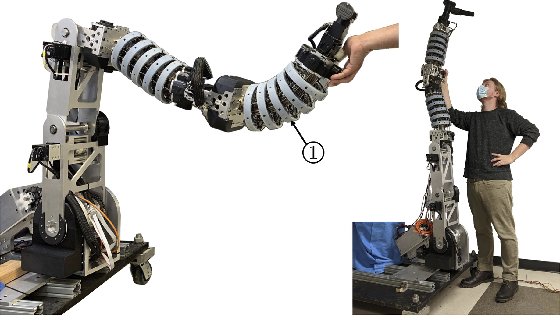
2. Related works
2.1. General contact estimation
In past works, to address the challenge of contact detection and estimation, other researchers have also incorporated sensors into robots in order to estimate the location and magnitude of the wrench applied during contact. Examples of this include sensory skins such as Yamada et al. (2005), Abah et al. (2019), and Abah et al. (2022), strain gauges placed onto the body of the robot as in García et al. (2003) and Malzahn and Bertram (2014), force/torque sensors in the robot’s wrist and/or base as in Lu et al. (2005) and Shimachi et al. (2008), vibration and acoustic analysis as in Richmond and Pai (2000), Min et al. (2019), and Fan et al. (2020), and joint torque sensors as in Popov et al. (2017).
Sensor-based methods can suffer from dead zones where sensors are not present and can be cost-ineffective. Therefore, researchers explored methods for contact detection that do not rely on adding extra sensors to the robot. The earliest technique is the joint force/torque deviation (JFD) method given in Takakura et al. (1989), Suita et al. (1995), Yamada et al. (1996), and Bajo and Simaan (2010). This method is also referred to as direct estimation by some authors (e.g., in Haddadin et al. (2017)). The JFD method consists of subtracting model-predicted generalized forces from the sensed generalized forces (e.g., using joint torque sensing). The model-predicted generalized forces may be from a full dynamic model as in Suita et al. (1995) or from a statics model as in Bajo and Simaan (2010). A model of the joint level friction is sometimes added to increase the accuracy of the method. The downside of this method is that it relies on joint-level current (or torque) sensing and is highly sensitive to the accuracy of the dynamic/static model. This can lead to false positives due to modeling errors and/or unmodeled friction. For methods that rely on the full dynamic model to predict the generalized forces such as Takakura et al. (1989), Suita et al. (1995), and Yamada et al. (1996), a numerical second-derivative of the joint positions is required which can lead to extremely noisy estimation signals. Additionally, JFD works best for slow motions where viscous friction and the effect of unmodeled dynamics are small.
Due to the aforementioned issues with estimation noise, it may be desirable to use methods that do not rely on the second derivative of the joint position and provide estimation noise filtering. These methods are based on the fault detection literature such as Wünnenberg and Frank (1990), Freyermuth (1991), Caccavale and Walker (1997), Hammouri et al. (1999), and De Persis and Isidori (2001) and typically rely on knowledge of the robot’s dynamic parameters. They work by observing an unexpected deviation in some aspect of the robot’s dynamic state such as its energy, joint velocity, or generalized momentum. A detailed review of these methods is given in Haddadin et al. (2017). The most common of these methods is the generalized momentum observer (GMO). This method was first developed in De Luca and Mattone (2003) and has been used in a wide range of applications such as flying robots in Tomić et al. (2017), humanoids in Vorndamme et al. (2017), redundant manipulators in De Luca and Ferrajoli (2008) and Cho et al. (2012), and robots with series-elastic actuators in De Luca et al. (2006) and Kim et al. (2015). The GMO has also been combined with Kalman filters in Wahrburg et al. (2015, 2018)bib_wahrburg_et_al_2018, additional sensory input in Buondonno and De Luca (2016), and friction models in Lee et al. (2015) and Lee and Song (2016) to improve the performance of the observer. The performance of the observer under characterized dynamic model uncertainty has also been studied in Briquet-Kerestedjian et al. (2017) and Li et al. (2021). It should also be noted that the GMO bares some similarities to the time-delay control paradigm introduced in Youcef-Toumi and Ito (1988) as it relies on previous measurements of the system state to estimate the contributions of external disturbances.
The GMO method for contact estimation has been used predominantly for rigid-link robots with/without series-elastic actuators. A detailed review of contact detection and localization methods for continuum robots is presented next in the related works section. Despite its successful use for various robot architectures, adapting the GMO method has not been previously applied to continuum robots. Furthermore, investigating the effects of state uncertainty on the performance of the contact estimator of a continuum robot has not been carried out.
The contribution of this paper is in presenting a modal space formulation of the GMO and verification of the GMO method to variable curvature continuum robots while taking into account uncertainty in the dynamic state of the robot. Unlike serial rigid-link robots, the shape of continuum robots is heavily dependent on external loading. To enable successful adaptation of the GMO method for continuum robots, one must overcome the challenge due to the load-induced shape changes. One, therefore, needs a modeling framework that takes this information into account. For these reasons, we leverage our recent result on real-time shape sensing in Orekhov et al. (2023) along with a dynamic formulation in the modal curvature space to present a formulation of the GMO method that can be used for continuum and soft robots. Relative to prior works in GMO-based contact estimation, we present a unique constrained optimization formulation for solving the problem of contact wrench estimation. We also present a model of the effects of dynamic state uncertainty on the output of the GMO and leverage this result to make recommendations for setting detection thresholds. Lastly, we compare the performance of the GMO to the performance of the JFD method in both simulation and experiment.
The next section presents related works while focusing on the most relevant works on contact detection/estimation for continuum robots. The following sections present the shape sensing approach and a dynamic formulation in the space of curvature modal factors. We then present an adaptation of the GMO method and an investigation of state parameter uncertainty on expected performance. Finally, sections 11 and 12 present a simulation-based study and experimental validation on the isolated distal continuum segment of the robot shown in Figure 1. Lastly, in section 13 we present a preliminary extension of the method to multisegment continuum robots.
2.2. Contact estimation for continuum robots
In addition to the seminal works on collision detection reviewed above, the most relevant work to this paper is De Luca and Mattone (2003), which we build on and extend in this paper. Within the scope of contact detection/estimation for continuum robots, the most relevant works are Xu and Simaan (2008), Bajo and Simaan (2010), Bajo and Simaan (2012), and Santina et al. (2020). In Bajo and Simaan (2010), the authors considered the JFD method and the effects of bounds of joint-force sensing uncertainty on the detectability of contact. In Bajo and Simaan (2012), a kinematics-based contact detection and localization approach based on motion tracking and detection in the shift of the instantaneous screws of motion was presented and shown to be quite effective for continuum robots that bend in circular shapes. Roy et al. (2016) simulated the effects of dynamics on this method assuming constant curvature bending profiles. In Rucker and Webster (2011), the authors combine Cosserat rod theory and extended Kalman filters to estimate the applied wrench to the tip of a continuum robot in quasi-static configurations. More recently, in Ashwin et al. (2021), the authors presented contact detection and estimation for wire-actuated continuum robots subject to quasi-static modeling assumptions. Lastly, in Leung et al. (2024), the authors present two tip-force estimation techniques for a two segment continuum robot using constant curvature assumptions. Their first technique uses a cantilever beam model to estimate the tip force and their second technique uses support vector regression to estimate the difference between no-load tendon forces and loaded tendon forces.
Table 1 summarizes the key modeling assumptions and capabilities supported by this work compared to the most relevant prior works. The limitations of these prior works on continuum robot contact estimation/detection are: ➣ The assumption of a known external load state (mostly unloaded) and known bending shape profiles of the continuum robot segments (e.g., most works in Table 1 assume constant curvature or use piece-wise constant curvature (PCC)). For example, Xu and Simaan (2008) assumed constant curvature and a force at the segment tip while Bajo and Simaan (2012) assumed constant curvature and detected contact along the length of a segment. Finally, Chen et al. (2021) assumed a planar curvature experimentally captured via a modal representation of the local tangent angle of a fiber-reinforced bellow actuator acting as a single-segment soft robot. ➣ The methods do not estimate the magnitude of the contact force and assume negligible dynamics. For example, Bajo and Simaan (2012) assumed negligible dynamics in their kinematics-based contact detection and localization approach. In Santina et al. (2020), the authors estimated contact forces in soft robots while assuming PCC, ignoring Coriolis/centrifugal and inertial effects, and assuming extrinsic sensing of the robot shape using optical tracking. Summary of the continuum robot contact estimation literature.
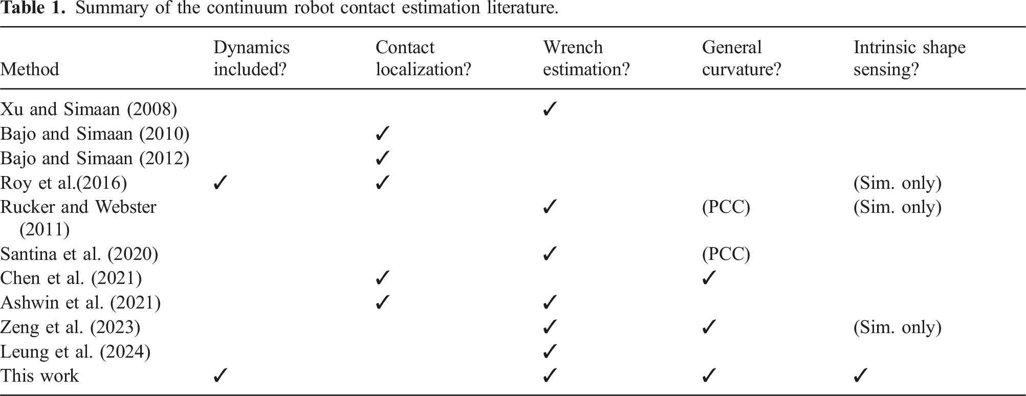
While these approaches can work very well for small continuum robots with negligible dynamics and gravitation-induced deflections, large robots such as in Figure 1 require special consideration of their dynamics and the ensuing shape deflections.
The goal of this work is to address the limitations of prior works as shown in Table 1 via an extension/adaptation of the GMO method to continuum robots subject to dynamic loading and with general bending shape profiles. The robot shown in Figure 1 is very large and therefore its segments undergo significant passive deflections violating the constant curvature assumptions. This robot is also designed to work within confined spaces where external optical tracking may not be possible, therefore a combined approach achieving intrinsic shape sensing, contact detection, and contact wrench estimation is sought in this work.
Another set of key works that we build on and extend is the literature on continuum robot dynamics and kinematics. In this work, we build on Chirikjian’s (Chirikjian and Burdick, 1994, 1995; Chirikjian, 1994) early works on modal space representation of hyperredundant robots. We present a modal-space dynamics model for the purpose of formulating the GMO contact estimation approach and analyzing the effects of uncertainty.
3. Problem definition and modeling assumptions
This paper focuses on presenting an extension of the GMO contact estimation method to continuum robots. Because these robots are very different from traditional serial rigid-link robots, these robots have significant sources of geometric, dynamic, and mechanics uncertainty. This combination of challenges requires solutions for online shape sensing, updated kinematics, and updated dynamics in a way that allows reliable application of the GMO algorithm. Therefore, the two problems targeted by this paper are: ➣ Collision Estimation: Detect contact and estimate the wrench applied to the robot during contact. ➣ Effects of Uncertainty: Formulate the effects of uncertainty and provide an estimate of the effects of uncertainty on the GMO estimator, thereby delineating the limits of contact detectability due to uncertainty.
In dynamics model presented in this paper, we make the following assumptions: ➣ The friction in the actuation tendons can be modeled as concentrated forces at the contact points between the actuation tendons and the robot body. ➣ The friction can be modeled as a smooth Coulomb friction model ➣ Viscous effects that may arise due to gearhead losses can be neglected ➣ The robot is torsionally rigid. This assumption is justified since the robot shown in Figure 1 has bellows with very high torsional stiffness as reported in Orekhov et al. (2023). ➣ The central backbone of the robot includes a superelastic nickel-titanium (NiTi) rod. NiTi is known to exhibit a nonlinear, hysteretic stress-strain curve (Liu et al., 1999). Because we mostly operate in the second stress-strain curve plateau that occurs past approximately 2% strain (Liu et al., 1999), we neglect these effects and assume a linear elasticity model for simplicity. ➣ Although the method can handle more complex contact types, we evaluate the method in simulation and experiment using only point contacts.
4. Modal kinematics
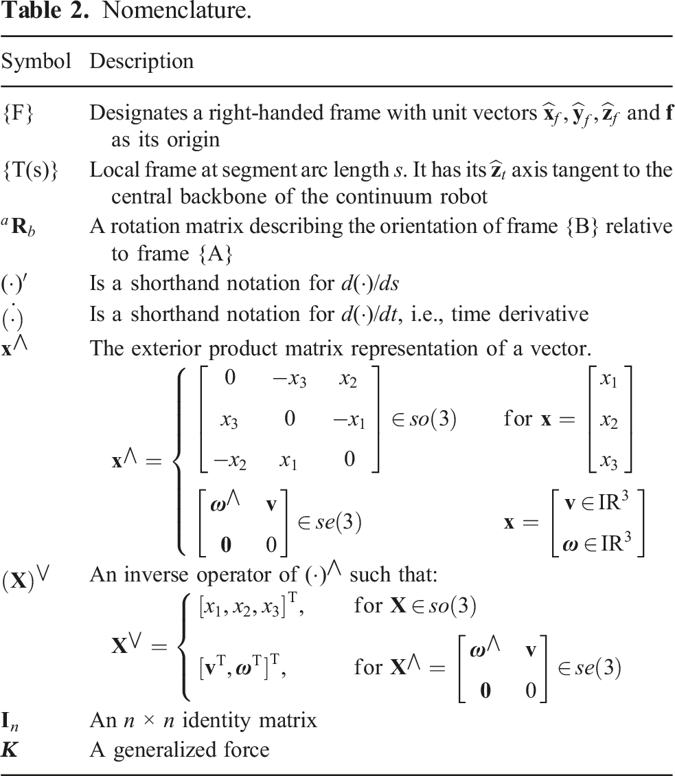
The instantaneous shape of the continuum segment shown in Figure 2 will be represented using a modal representation following the model presented in Orekhov et al. (2023). For completeness, we briefly summarize the modal kinematics below while using the nomenclature presented in Table 2. (a) Actuation tendons and passive shape sensing strings whose lengths are used to calculate Nomenclature.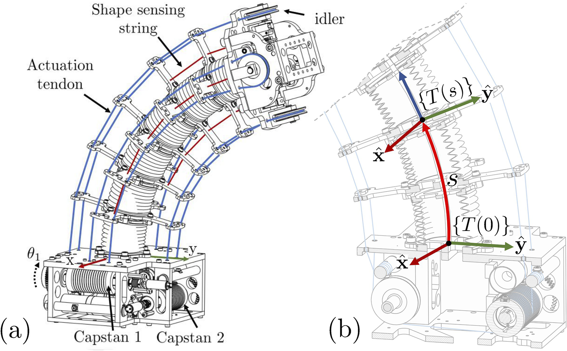
The continuum segment of Figure 2 uses two capstans with two fixed-length wire loops to bend in any direction. The robot uses torsionally rigid metal bellows assembled on a superelastic NiTi rod. Since the bellows are torsionally very stiff, we assume the robot does not experience torsional strains and that the robot has a fixed arc length L. For a given arc length s ∈ [0, L] along a continuum segment, a local frame 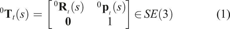
As the robot undergoes a deformation parameterized in the local frame as a twist 
The body twist 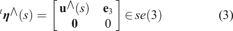
In this work, we choose to represent 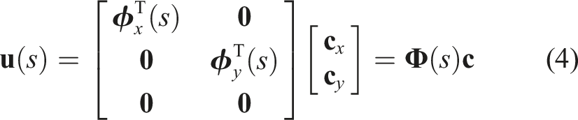
We chose these polynomial basis functions to be the first three Chebyshev polynomials of the first kind: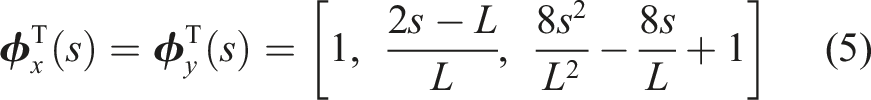
Chebyshev polynomials of the first kind were chosen over a simple monomial basis because Chebyshev polynomials are bounded to within ±1 and therefore improve scaling of the modal coefficients. Additionally, monomial bases are known to suffer from poor conditioning at higher powers as shown in Gautschi (1975). For a discussion on how the choice of Chebyshev polynomial order affects the accuracy of the kinematics model see Orekhov and Simaan (2020).
4.1. Shape sensing
As shown in Figure 2, the robot used in this work is endowed with four string encoders that measure the change in arc length between the end-disk and one of the spacer disks. As reported in Orekhov et al. (2023), these string encoders are custom-made using Renishaw AM4096 12 b incremental rotary encoders. These custom-made string encoders have an average measurement error of 0.1 mm (0.08% of the total stroke) and a maximum error of 0.27 mm (0.23% of total stroke). Using the string encoder measurements, as well as the change in backbone lengths, we can calculate the modal coefficients 
Because the robot used in this paper is torsionally stiff and has constant pitch-radius string encoder/actuation tendon routing,
4.2. Modal body Jacobian
In this section, we will derive the Jacobian
The body twist of the end-effector can be found using:
After integration of (2), 
To calculate (9), we must compute the partial derivative of
4.3. Modal capstan Jacobian
In this section, we will derive the Jacobian 
5. Continuum robot dynamics in the space of modal coefficients
Since the GMO method requires the robot’s dynamics, the dynamics of the continuum segment shown in Figure 2 is derived in the space of modal coefficients using the Euler–Lagrange method. The closest work to this section is the work of Roy et al. (2016). However, the dynamic model presented in Roy et al. (2016) assumes constant curvature (i.e., circular) bending. In this section, we will relax this assumption. The derivations provided in sections 5.1 and 5.2 are extended to general curvature from the constant-curvature models presented in Roy et al. (2016). The friction model presented in section 5.3 is unique to this paper.
5.1. Kinetic energy
The total kinetic energy of the robot can be modeled as the sum of the central backbone’s kinetic energy T
CB
, the kinetic energy of the spacer disks T
SD
, and the kinetic energy of the actuation capstans and motors T
A
.
The models presented in sections 5.1.1 and 5.1.2 are adapted to general curvature from the constant curvature models presented in Roy et al. (2016). However, the derivations provided in section 5.1.3 are unique to this paper.
5.1.1. Central backbone
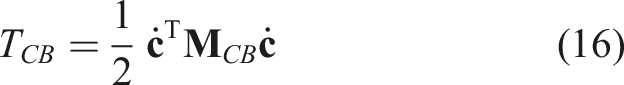
The kinetic energy of the central backbone can be found using the robot body twist coordinates 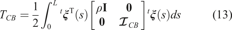
In this equation, 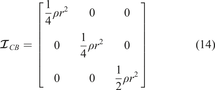
Using the modal Jacobian matrix 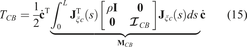
5.1.2. Spacer disks
In the following, we define for each spacer disk the local backbone frame {T
Using 
Using 
5.1.3. Actuation capstans and motors
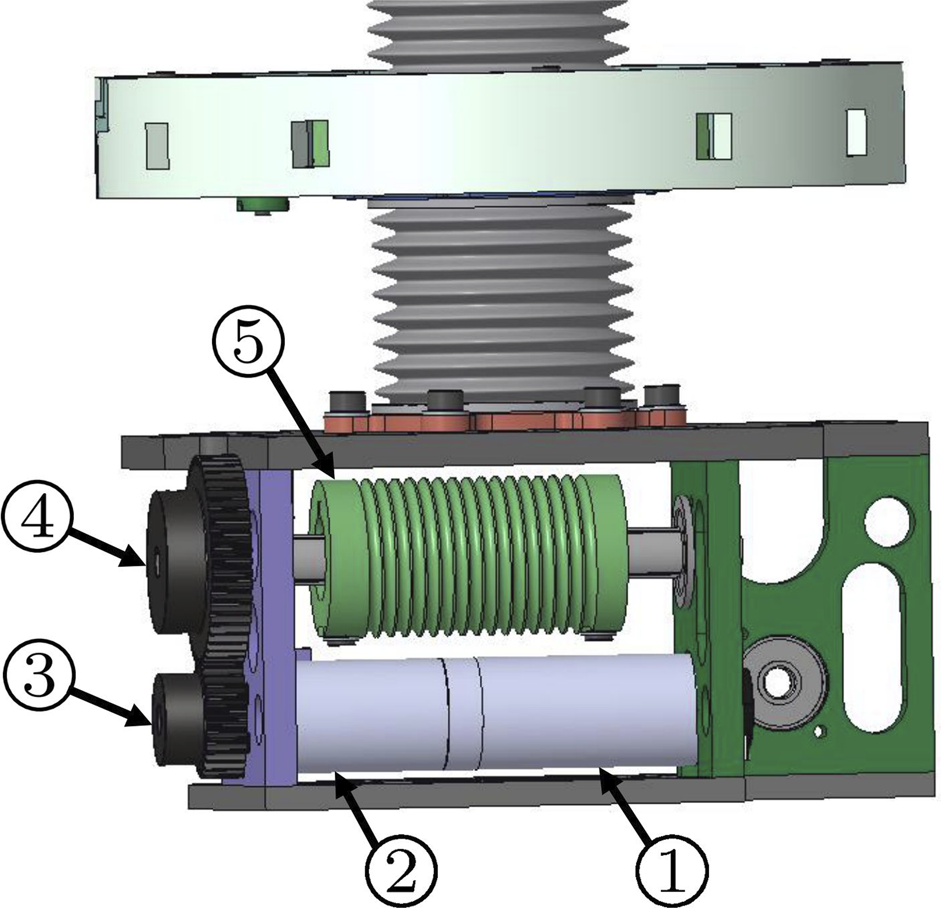
Each axis of the continuum robot actuation unit consists of a motor (Figure 3①) with rotor inertia J
m
attached to gearhead (Figure 3②) with inertia J
gh
as viewed by the gearhead input and reduction ratio R
gh
. The gearhead is attached to a pinion (Figure 3③) with inertia J
p
which meshes with a gear (Figure 3④) with inertia J
g
. The gear is rigidly attached to a shaft and capstan (Figure 3⑤) with combined inertia J
c
. Using this information, the inertia of the entire actuation chain as viewed by the capstan can be written as: Continuum robot actuation unit: ① Motor with rotor inertia J
m
, ② gearhead with inertia J
gh
and reduction ratio R
gh
, ③ pinion with inertia J
p
about the center of rotation, ④ gear with inertia J
g
about the center of rotation, and ⑤ shaft and capstan with combined inertia J
c
. The gear and pinion have a reduction ratio of R
gp
.
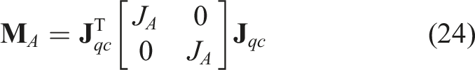
The kinetic energy of the capstans T
A
can be found using J
A
and the angular velocity of the capstans 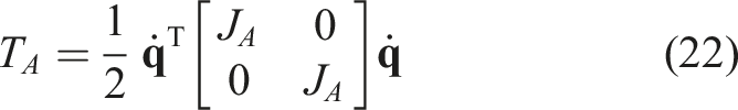
T
A
can be written in terms of the modal coefficient rates using: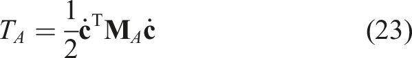
Using (16), (19), and (23), the total kinetic energy of the continuum robot can be written as: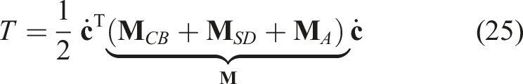
Note that, in reality, the capstans also slowly translate along their supporting shafts as they rotate. The kinetic energy from this effect is ignored in this model.
5.2. Potential energy
The total potential energy of the robot can be modeled as the sum of the bending energy V
B
of the central backbone, the gravitational potential energy of the central backbone V
CB
, and the gravitational potential energy of the spacer disks V
SD
.
The derivations given in this section are extended to general curvature from the constant curvature models presented in Roy et al. (2016).
5.2.1. Elastic potential energy
The bending stiffness matrix of the central backbone can be written as:
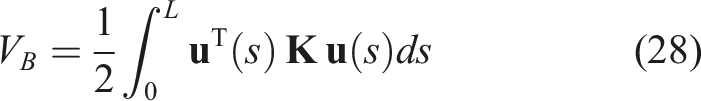
Using (4), V
B
can be written in terms of 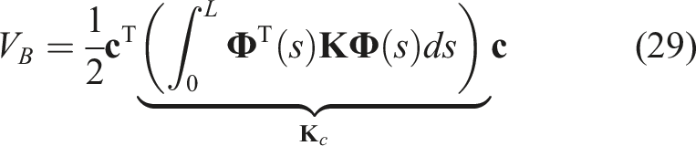
5.2.2. Gravitational potential energy
The gravitational potential energy of the central backbone can be written as: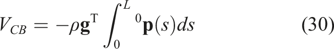
The gravitational potential energy of the spacer disks can be written as: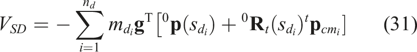
5.3. Approximate joint friction
In this section, we will approximate the effect of friction between the actuation tendons and the brass bushings that guide the actuation tendons through the spacer disks. Our approach, which is unique to this paper, uses a simplistic Coulomb friction model that ignores nonlinear, velocity-dependent effects such as Stribeck and viscous friction. As shown in Figures 2 and 4, the robot’s actuation tendons are wrapped around a motorized capstan and then routed through holes in the spacer disks. Once the tendon reaches the end-disk, they are rerouted back through the spacer disks using a pulley (see Figure 2) and terminated on a fixed shaft. This is repeated on the same capstan, but separated by 180° to control bending in both directions in the same plane. To ensure the tendons are always in tension, each side of the tendon are pre-tensioned to f
pl
= 208 N. Continuum segment cross section showing the terms used to calculate the joint friction.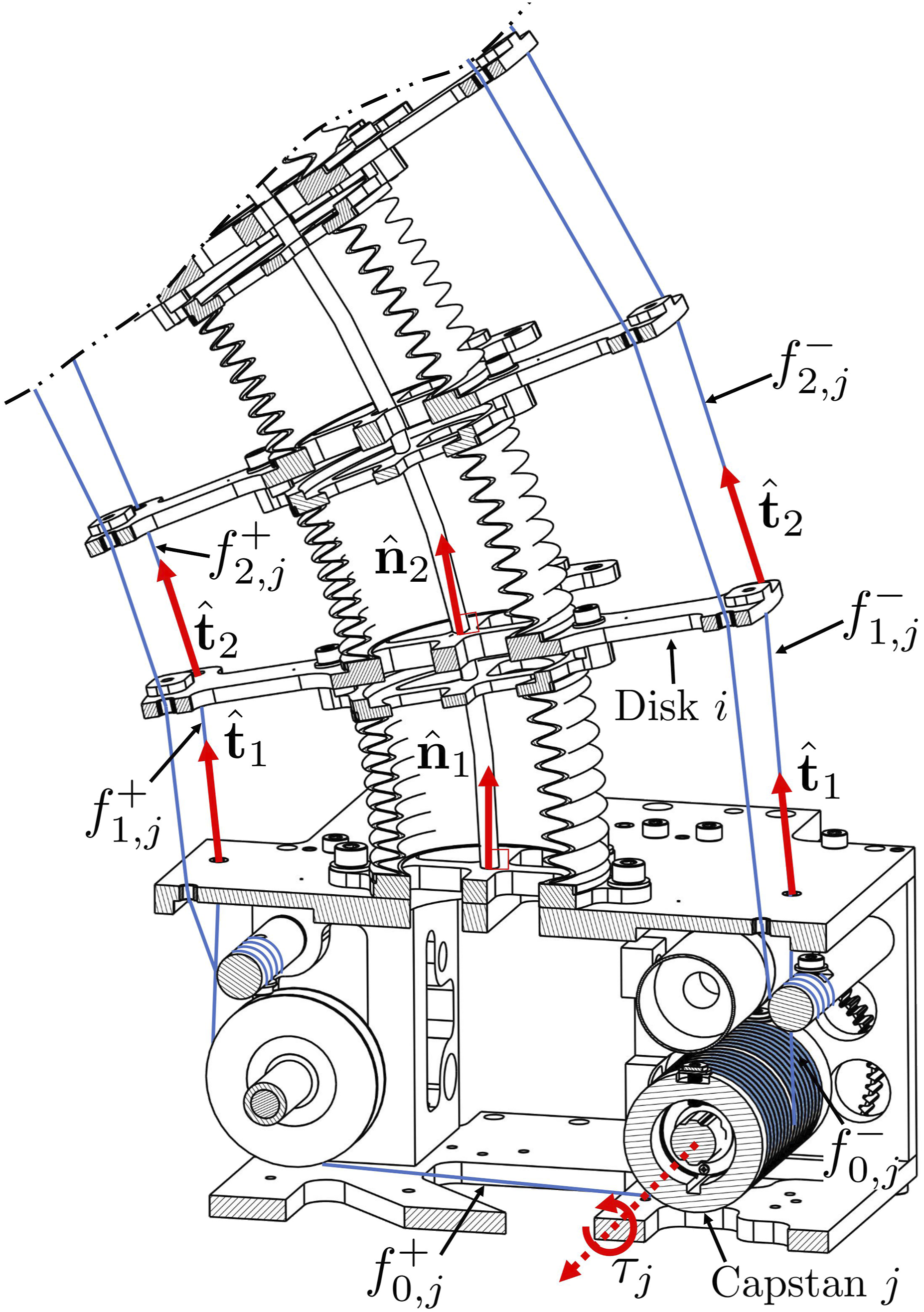
The pretensions cannot create a moment about the capstan because they act in equal and opposite directions on the capstan.
1
The pretension does, however, affect the friction between the tendons and the bushings because it contributes to the normal force. When torque τ
j
is applied to capstan j ∈ [1, 2], the tension in the tendon being pulled by the capstan is 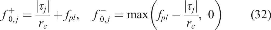
As the tendon passes through the bushing in disk i, the tendon tension is reduced by the friction force between the bushing and the tendon (
In this section, we will use the convention that i = 1 at the segment base as shown in Figure 4. The friction forces depend on the magnitude of normal force between the tendon and the bushing (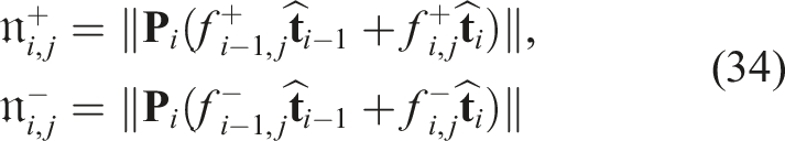
Given the tension 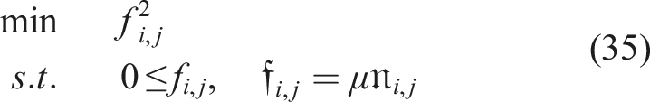
This optimization problem must be solved starting from i = 1 (i.e., the segment base) and progressing at each section of tendon until the end-disk and back from the end-disk to the termination point. In our approach, the constrained minimization problem given in (35) is solved using the sequential quadratic programming algorithm implemented in MATLAB’s fmincon function. At each disk, after
Once the friction force at each bushing is known, the total friction force experienced by capstan j is the sum of each value of 
The torque on the capstans due to friction can now be found using the capstan radius r
c
:
For the purposes of simulation, the 
5.4. Equations of motion
Using the total kinetic energy of the segment from section 5.1 and the total potential energy of the segment from section 5.2, the Lagrangian 
Using 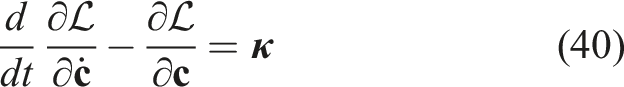

In this equation, 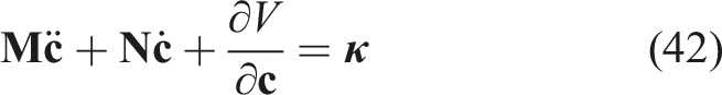
6. Modal-space momentum observer collision detection
6.1. Observer formulation
In this section, we adapt the momentum observer framework presented in De Luca and Mattone (2003) to our modal approach and present our implementation of the observer. The momentum observer approach relies on a detection of a change in the robot’s generalized momentum as a means to detect an incident of collision. The generalized momentum 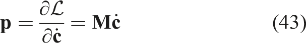
Since the contact impulse is related to a temporal change in momentum, we calculate 
Substituting the solution for 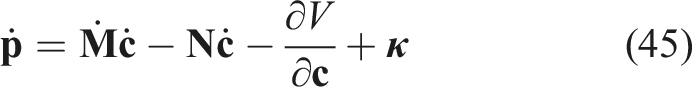
Since the matrix 
Using this result along with (41), equation (45) can now be expressed as: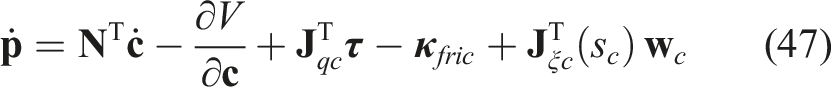
Since we do not know the contact wrench 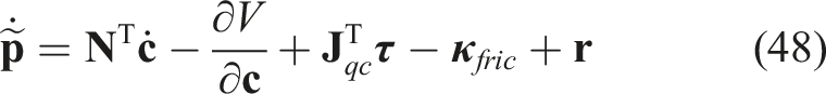
In the following derivation, we assume that a contact estimation algorithm is updated at every sensory acquisition cycle i, but the value of 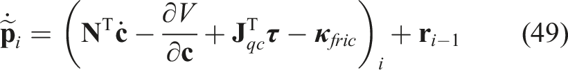
To reject sensory noise, we assume that 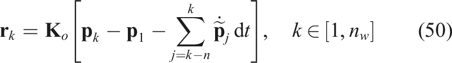
In the above definition, dt is the sensory update cycle time, n
w
denotes the total number of cycles where the estimator is allowed to run before it is reset. This is needed to avoid false positives due to cumulative summation/integration effects of measurement noise and model error. The matrix
Substituting (49) in (50) results in the explicit form of the update law for the residual: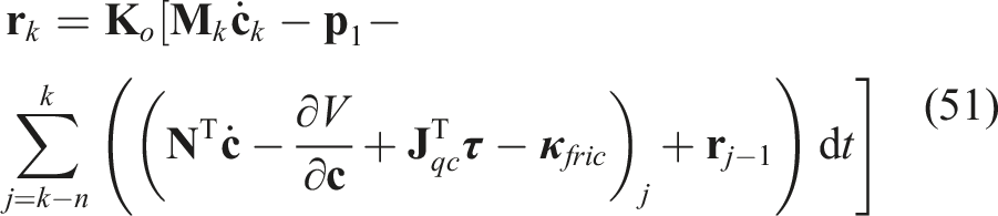
6.2. Estimator dynamics and stability
In this section, we will repeat a result first introduced by De Luca and Mattone (2003) which proves that the GMO is a stable, first-order, filtered estimate of the generalized forces due to contact. To investigate the estimation dynamics, we will cast (50) into the continuous time domain and then take the derivative with respect to time: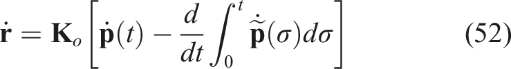
This equation simplifies to: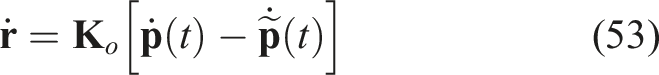
Plugging (45) and (49) in for 

Solving for κc,i yields: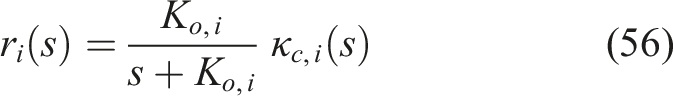
This equation can be re-written to reveal the time constant of the filter: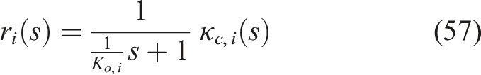
As shown in De Luca and Mattone (2003), for a positive estimation gain Ko,i > 0, the transfer function r i (s)/κc,i(s) given in (57) has one stable (i.e., negative) pole at s = −Ko,i. Therefore, in ideal scenarios, the estimation signal r i will approach the true generalized force κc,i with time constant 1/Ko,i. From this analysis, it can be seen that selecting a gain is a balancing act between responsiveness of the estimator and noise filtering. Selecting a higher Ko,i value will create a more responsive estimator, but the estimator will be more sensitive to noise. Conversely, a lower gain will more effectively filter noise, but will have a delay in the estimation.
7. Wrench estimation
The output of the momentum observer 
In scenarios where the location of contact is known (e.g., from a sensor Abah et al. (2019; 2022)) and
7.1. Constrained minimization-based wrench estimation
However, the continuum segment shown in Figure 2 cannot instantaneously translate along the local 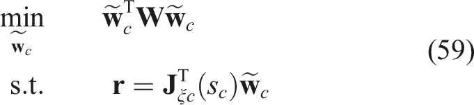
In this equation,
7.2. Incorporating knowledge of the contact type
In some scenarios, information about the type of external contact is known which imposes constraints on the components of the applied wrench. For instance, if the contact is assumed to be a point contact, it cannot impart a moment to the segment and the moment components of 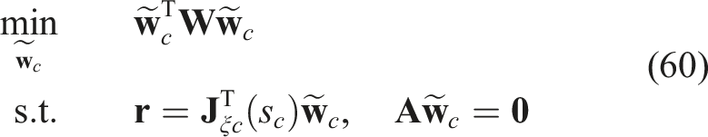
For the simulations and experiments in this paper, the applied wrench is assumed to be a point contact and the force along the local z axis is assumed to be zero for the reasons described above. Therefore, we will use the following 
For the simulations and experiments in this paper, (60) was implemented in MATLAB 2023a and was compiled using MATLAB coder. During the experiments shown in Figure 9(a), (60) was solved with a median execution time of 0.0390 seconds and a maximum execution time of 0.1297 seconds. The computer used for this analysis has 32 GB of RAM and an Intel™ i7-13700 processor. The operating system was Windows 10.
8. Effect of state uncertainty on wrench estimation
In the following, we consider the effect of parameter and model uncertainty on the GMO method. Understanding how uncertainty in the segment’s dynamic state affects the output of GMO is critical to characterizing the expected performance of the method. We therefore investigate how an unmodeled error in the state vector will affect the GMO residual.
Since our formulation is in modal space, we define the segment state vector as:
The effect of an unmodeled change Δ
In this work, we will approximate the effect of an unmodeled deviation in dynamic state Δ
The derivative of 
First, we will calculate d
Note that in this equation and the subsequent analysis, the subscript k, indicating the sample number, has been dropped for clarity. Using this summation representation of 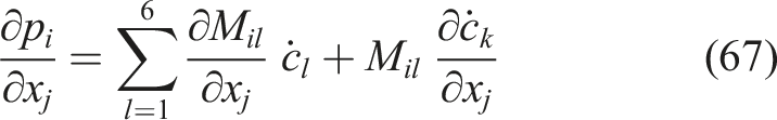
In our implementation, the partial derivatives of the elements of 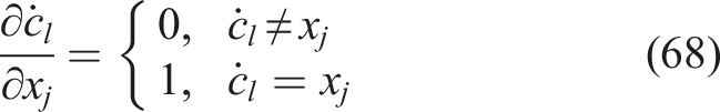
Next, we will compute the derivative of 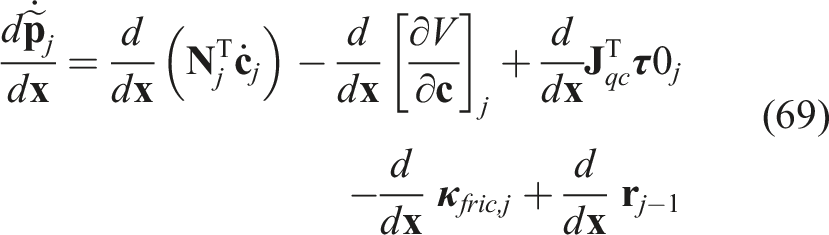
Because
Given a characterized uncertainty in
9. Joint force/torque deviation
One intuitive method for contact detection/estimation is the joint force/torque deviation (JFD) method. This method was proposed in some of the earliest works on robot contact estimation (e.g., Suita et al. (1995)) and has been applied to continuum robots for contact detection for static scenarios in Bajo and Simaan (2010). This method is also referred to in the literature as the direct estimation method (e.g., Haddadin et al. (2017)). The key idea of this method is to rearrange the robot’s full dynamic model (42) to directly solve for the generalized forces due to contact: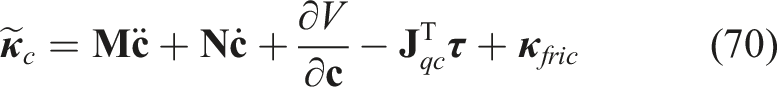
Using
In the experimental evaluation section of this paper, the JFD method is used as a baseline of comparison for the performance of the GMO.
10. Dynamic model calibration
Dynamic model parameters.
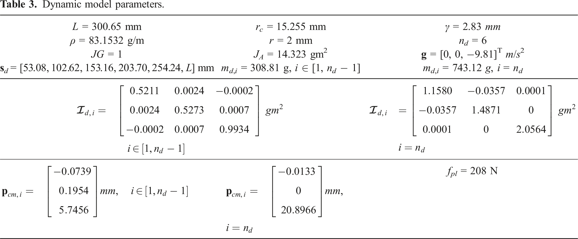
To calibrate these parameters, the segment’s capstans were commanded to move with a chirp trajectory that starts from f1 = 0.01 Hz and linearly increases to f0 = 0.25 Hz in t
f
= 6 seconds, has an amplitude of qmax = 360° (which corresponds to 42 degrees of segment bending), and a phase offset of ϕ0 = 90°. The chirp trajectory is given by: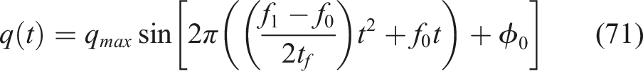
During the experiment, the string encoders were read using a Teensy 4.1 microcontroller and sent to the central control computer using user datagram protocol (UDP) communication. For more information on the string encoders see Orekhov et al. (2020, 2023). The segment’s motors (Maxon™ DCX22L GB KL) were controlled using Maxon™ ESCON 50/5 motor drivers, Sensoray™ 526 encoder reading cards, and a Diamond Systems™ Aries PC/104 CPU running Ubuntu 14.04 with the PREEMPT-RT real-time patch. The segment motors were current controlled and the commanded current was used to estimate the capstan torque using the motor’s torque current constant, the rated efficiency of the motor and gearhead (Maxon™ GPX22HP 62:1), and the reduction ratios of the gearhead and the additional gearing (Figure 3③ and ④). The encoders and capstan torque readings are sent to the central control computer using UDP communication. The central control computer runs Ubuntu 18.04 with the Melodic distribution of the Robot Operating System (ROS). For the duration of the experiment, data was recorded from the motor encoders, motor torques, and string encoders using ROS topics at an average sampling rate of ∼100 Hz.
Using the recorded starting pose of the segment and the recorded capstan torques, the segment’s motion was simulated using MATLAB’s implementation of the Dormand–Prince version of the Runge-Kutta method (ode45) first described in Dormand and Prince (1980). Using the recorded modal coefficients from this experiment, the backbone flexural rigidities and friction coefficients were calibrated using the following constrained minimization problem: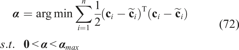
Calibrated dynamic model parameters.
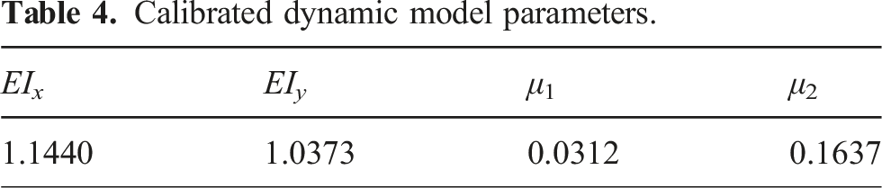
Figure 5 compares the simulated and experimental x, y, and z components of the segment tip position Simulated versus measured continuum segment tip positions after calibration: ① Experimental tip x position, ② simulated tip x position, ③ experimental tip y position, ④ simulated tip y position, ⑤ experimental tip z, and ⑥ simulated tip z position.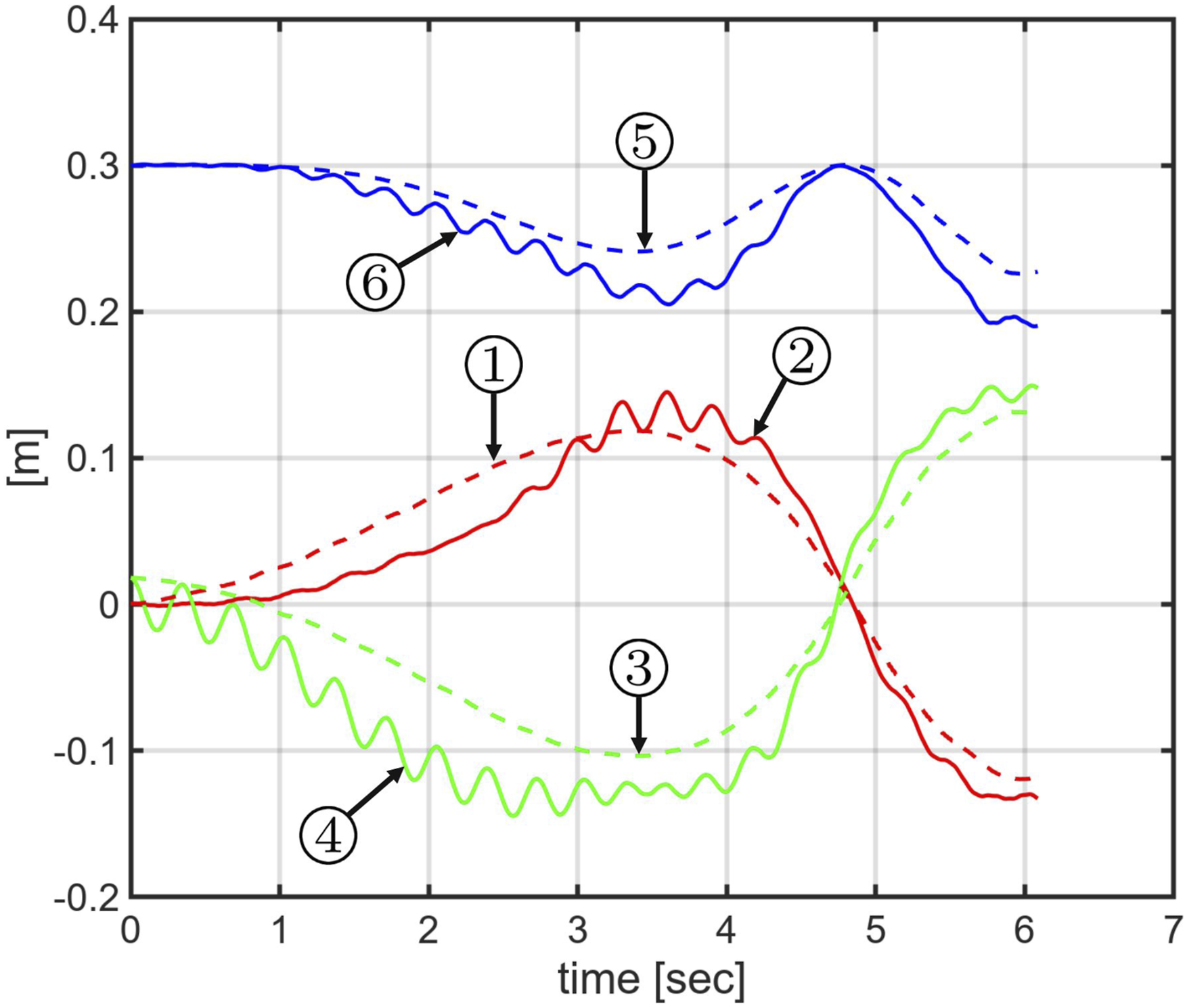
Other than the errors in the dynamic model, potential sources of error in this experiment include the use of commanded current to estimate the applied torque (the actual current supplied to the motor may differ from the command), the lack of exact data synchronization inherent in the decentralized structure of the control framework, errors due to numerical differentiation of the modal coefficients, backlash in the drive train, and sensor noise. Another major source of error was the shape sensing approach first presented in Orekhov et al. (2023). In this paper, the authors report an average end-disk positional error of 5.9 mm (1.9% of L) and a maximum error of 14.4 mm (4.8% of L).
11. Simulation studies
11.1. Effect of state-uncertainty
To investigate the effects of state uncertainty on the output of the momentum observer and the joint force/torque deviation method, we generated 21 body frame wrenches with x and y forces ranging between ±50 N. For each wrench, we also generated capstan torque values ranging between ±2 Nm. Using MATLAB’s implementation of the Dormand–Prince version of the Runge-Kutta method (ode45) (Dormand and Prince (1980)), the segment’s motion was simulated for 1 second for each randomly generated applied wrench/capstan torques. The simulations were started with the segment in the straight configuration and the applied wrench and capstan torques were increased from zero to the generated value over the 1 second simulation. The wrench was applied to the tip of the continuum robot (s
c
= L). For each of the 21 generated wrenches, the applied wrench was estimated with constant errors in the state vector ranging from a 0% to 20% in steps of 2.22% for a total of 210 simulation conditions. For the GMO, the observer gain used in the simulation was
The results of these simulations are shown in Figure 6 and Table 5. Figure 6 shows polar scatter plots of the simulation results. Figure 6(a) shows the results for the GMO and Figure 6(b) shows the results for the JFD method. In both plots, the radial coordinate indicates the RMSE in the estimated force magnitude Simulation results: (a) GMO and (b) JFD. In both plots, the radial axis shows the RMSE in the sensed force norm w
e
, the angular axis shows the RMSE in the estimated wrench direction θ
e
, and the color of the data points represent the percent error in the state vector. Simulation results: Mean and max estimated force RMSE values at representative state vector percent errors.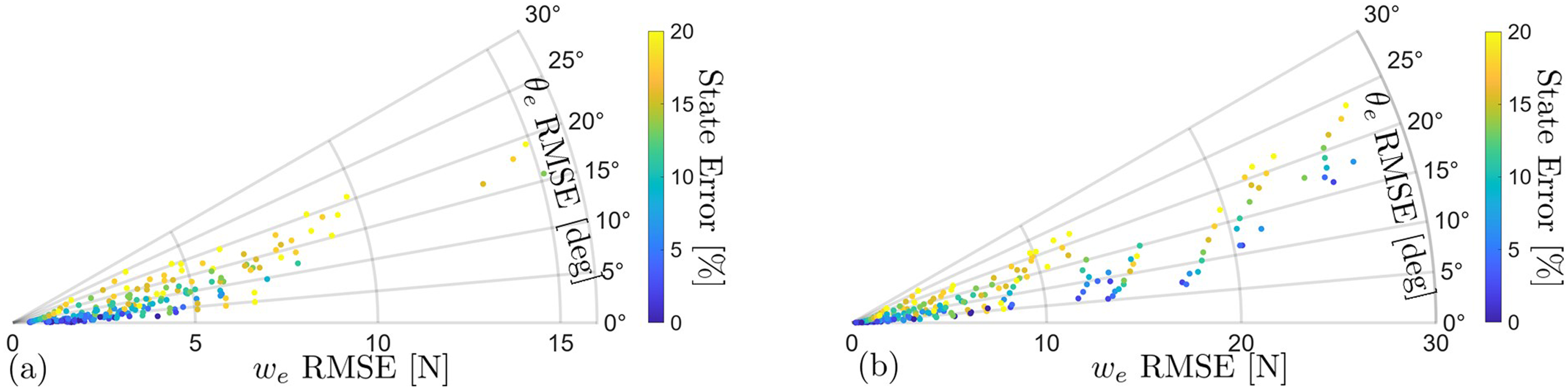
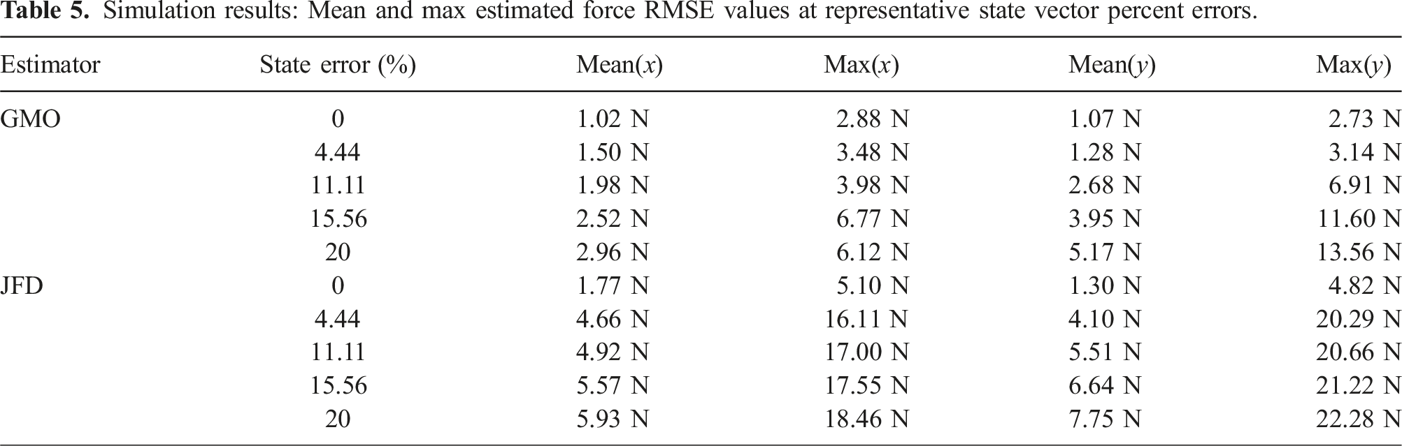
Table 5 shows the mean and max RMSE values at representative percent errors in the state vector. These results indicate that, assuming the applied forces are bounded to ±50 N and the error in the dynamic state is bounded to 20%, the average RMSE in the GMO force estimation is expected to be around 2.96 N in the x direction and 5.17 N in the y direction. The RMSE can be expected to be below 6.12 N in the x direction and 13.56 N in the y direction. For the JFD method, the average RMSE can be expected to be around 5.93 N in the x direction and 7.75 N in the y direction. The RMSE for the JFD method can be expected to be at or below 18.46 N in the x and 22.28 N in the y.
The largest reason for the difference between the errors in the GMO and JFD method is the need for a numerical second derivative of the modal coefficients which introduces additional errors into the system. In these simulations and the experiments in section 12, the estimation errors for forces in the x direction are lower than in the y direction. There are many sources that contribute to this difference. The biggest contributors are the difference between the calibrated flexural rigidities and friction coefficients in Table 4. Additionally, there is small difference in the elements of
11.2. Effect of sensor noise
As previously stated, a major advantage of the GMO is the ability to filter sensor noise. In this section, we present a simple simulation study showing how sensor noise affects the performance of the GMO and JFD methods. In this simulation study, we simulated the dynamics of the robot for a two second interval. During the first second, Effect of sensor noise simulation results: (a) GMO with no sensor noise. (b) JFD with no sensor noise. (c) GMO with 0.001 peak-to-peak amplitude random noise added to 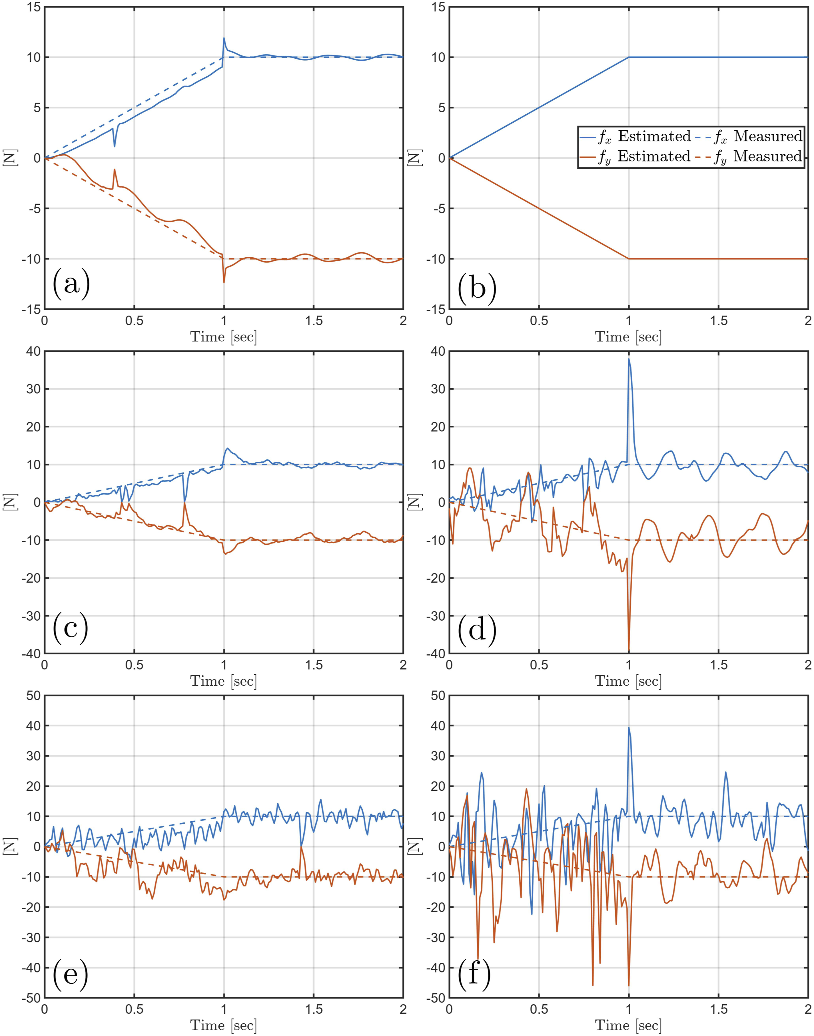
Sensor noise simulation results for GMO and JFD at increasing noise levels.
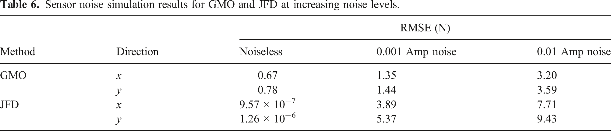
As can be seen in Figure 7 and Table 6, when the state vector and dynamic parameters are known exactly, the JFD perfectly predicts the applied wrench to within numerical precision. On the other hand, the GMO has small differences in the estimation mostly due to the sensing delay and estimator dynamics as discussed in section 6.2. However, when noise is introduced into the simulation, the GMO becomes more accurate for two primary reasons: (1) as discussed in section 6.2 the GMO acts as a low-pass filter and (2) the GMO does not require the numerical second derivatives of
12. Experimental evaluation
In order to experimentally validate our method and investigate how the speed, location, and direction of contact affects the results, we mounted a Bota Systems™ Rokubi force/torque sensor (Figure 8①) in a known location relative to the continuum segment such that the positive z axis of the force/torque sensor aligned with the positive x axis of the segment base frame {T(0)}. The force/torque sensor was positioned such that the tip was barely touching the center of first spacer disk. The segment was then commanded to move away from the sensor with capstan velocities Film strip showing an example of the experimental results given in Table 7: ① Bota Systems™ Rokubi force/torque sensor. Experimental test cases and results. The highlighted column indicates the experiment that was plotted in Figure 9.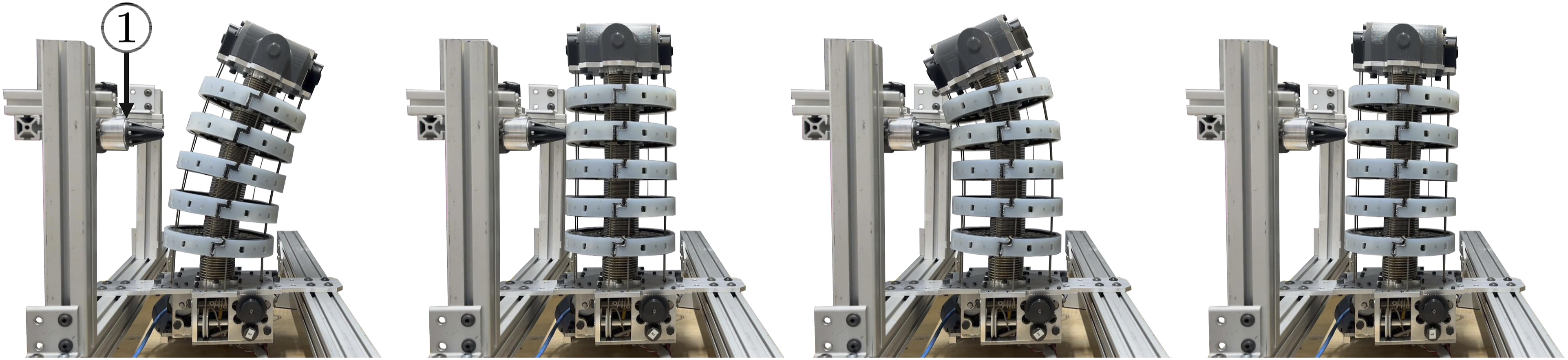
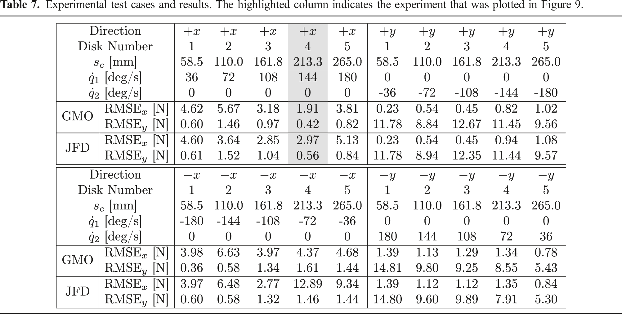
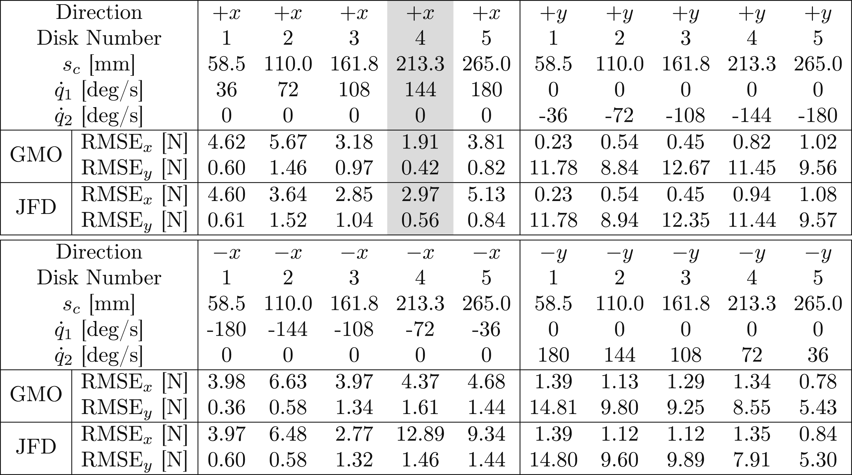
In the experiments, the modal coefficients
For the GMO, the residual gain was Plots showing an example of the experimental results given in Table 7. This is the same experiment shown in Figure 8. (a) The measured versus GMO-estimated applied force in the local disk frame. (b) The measured versus JFD estimated applied force in the local disk frame. (c) The GMO-estimated generalized forces 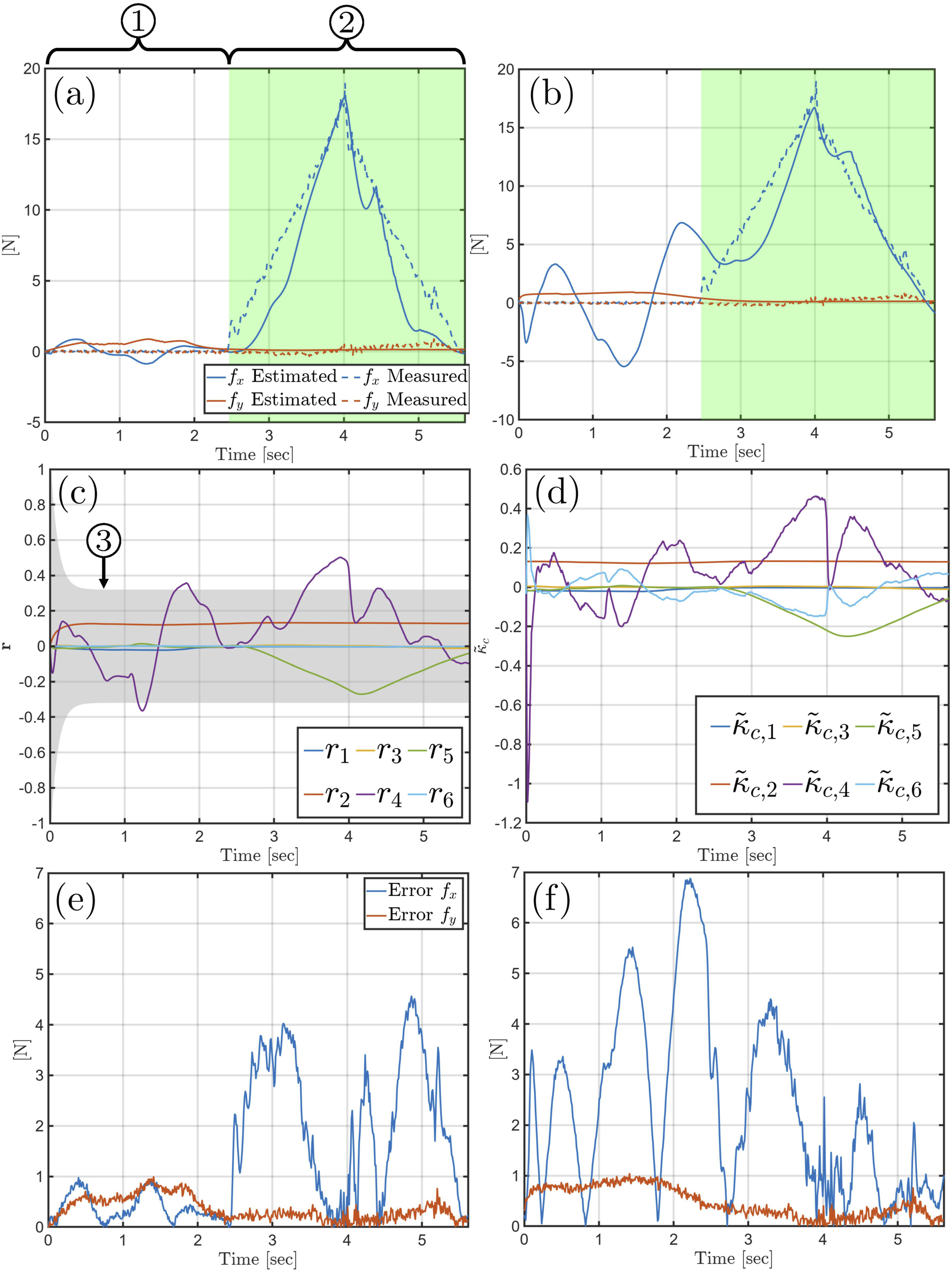
For the JFD, a 200 point, backwards-facing Gaussian filter was applied to both the estimated generalized forces
The shaded region of Figure 9(c) labeled ③ shows the threshold on the elements of
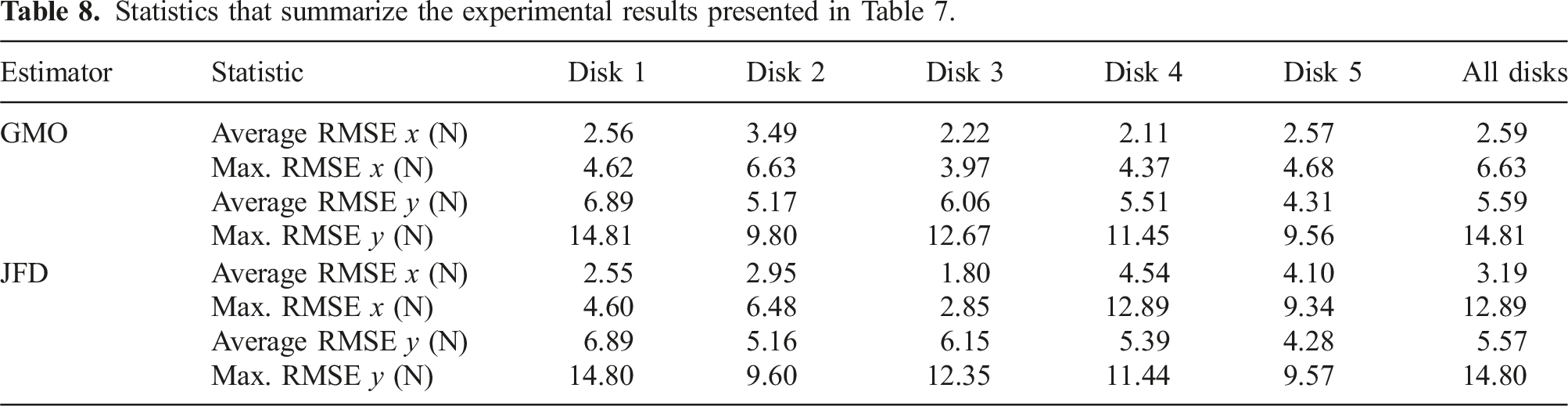
Statistics that summarize the experimental results presented in Table 7.
The vast majority of prior works on continuum robot contact detection assume a constant curvature (i.e., circular) bending model. A key contribution of this paper is a method for robots that do not bend in constant curvature arcs. To demonstrate that the robot did not bend in constant curvature during the experiment shown in Figure 8, we introduce a simple measure of how non-circular the robot was bending at any given time. First we define, the maximum curvature along the robot’s arclength, umax = max(u(s)), s = [0, L], and the minimum curvature along the robot’s arclength, umin = min(u(s)), s = [0, L]. The measure β is simply:
The closer β is to zero, the better the robot’s bending can be approximated by a circular arc. Figure 10(a) shows the maximum curvature during the experiment shown in Figure 8. Figure 10(b) shows the circular-ness measure β during the experiment.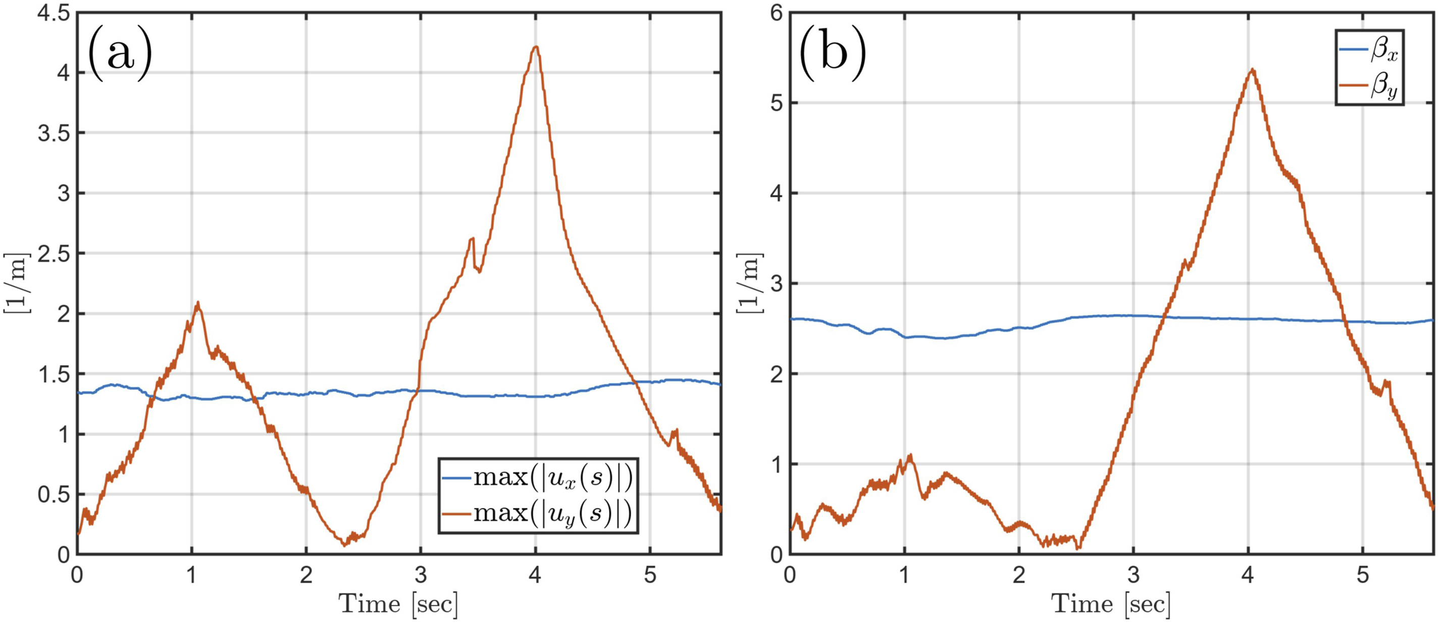
13. Preliminary experimental extension to multi-segment continuum robots
The results given in the previous section were for the distal segment in isolation. In this section, we will show preliminary results extending the method to the multisegment continuum robot shown in Figure 1. To do this, we must first discuss how the reaction moments from the distal segment’s actuation affects the dynamics of the proximal segment.
13.1. Reaction wrenches on the proximal segment
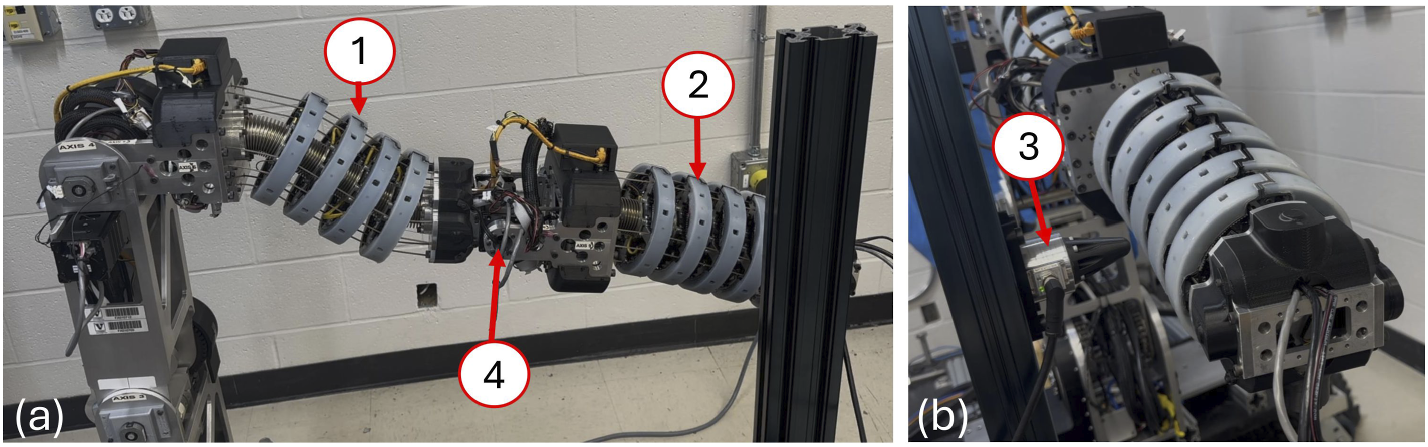
In these experiments, the mass and inertia of the distal segment was statically lumped into the end-disk. Additionally, the proximal segment must resist the reaction moments from the distal segment’s actuation motors as well as the reaction moment from the elbow motor placed between the two segments (see Figure 11④). To include these moments, we included the generalized forces due to the distal segment, Multisegment experimental setup. (a) Robot at its starting configuration. (b) Close-up of the contact point. ① Proximal segment, ② distal segment, ③ Rokubi force/torque sensor, and ④ elbow motor between segments. Videos of these experiments are provided in multimedia extension II.
To calculate 
In these equations,
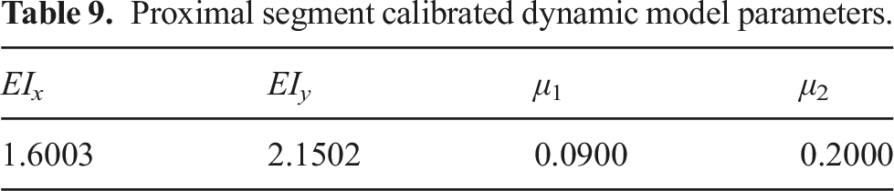
13.2. Proximal segment calibration
Proximal segment calibrated dynamic model parameters.
13.3. Experimental setup
In these experiments, we placed the continuum segments in a horizontal configuration as shown in Figure 11 (
In the experiments, the robot came into contact with the 4th spacer disk of the distal segment s c = 213.293 mm. The observer gains and filter windows were the same as the single-segment experiment.
13.4. Results
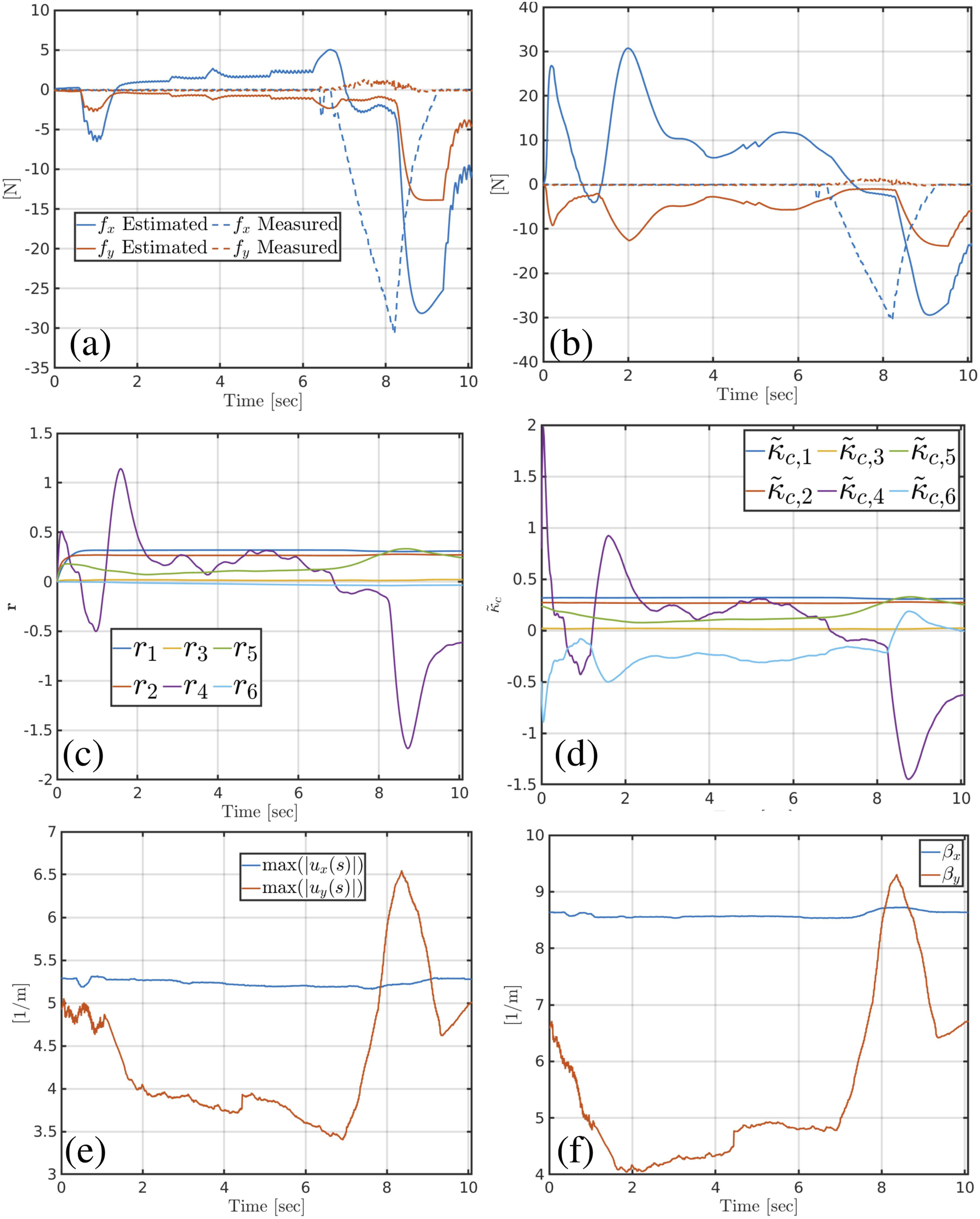
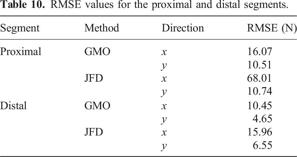
Figure 12 shows the experimental results for the proximal continuum segment and Figure 13 shows the results for the distal segment. In both figures, (a) shows the estimated wrench using the GMO and (b) shows the estimated wrench on the proximal segment using the JFD. Subfigures (c) and (d) show the estimated generalized forces due to contact for the GMO and JFD methods, respectively. Lastly, (e) shows the maximum curvature during the experiment and (f) shows the circular-ness measure during the experiment. Table 10 shows the estimation RMSE for the distal and proximal segments using both the JFD and GMO methods. Experimental results for the proximal segment. (a) Estimated forces in the x and y directions using the GMO. (b) x and y directions using the JFD. (c) GMO-estimated generalized forces Experimental results for the distal segment. (a) Estimated forces in the x and y directions using the GMO. (b) x and y directions using the JFD. (c) GMO-estimated generalized forces RMSE values for the proximal and distal segments.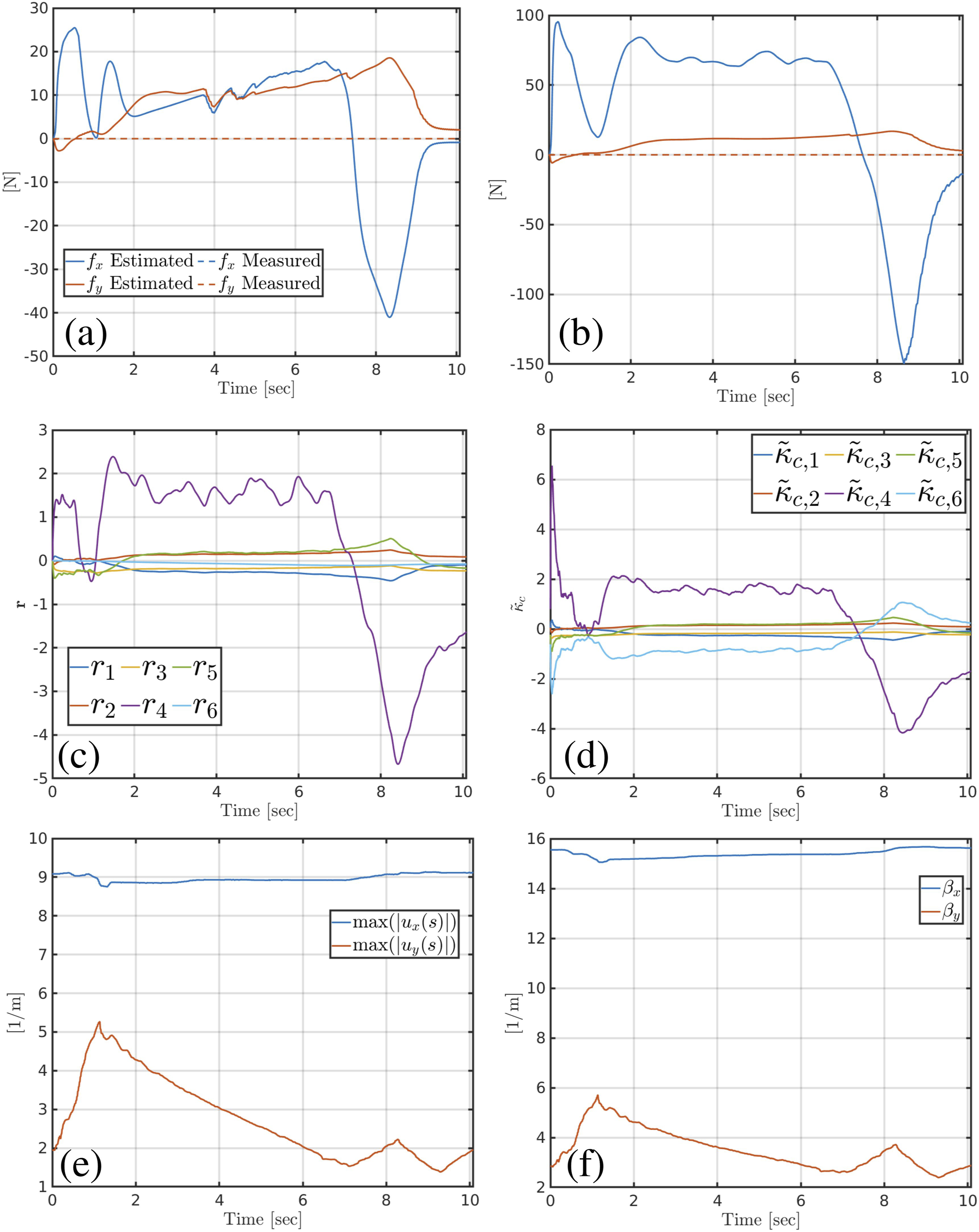
13.5. Discussion and limitations
As can be seen in Figure 11, the proximal segment is bent in a noticeable S-curve shape. This shape could not be reasonable approximated using a constant curvature assumption. In these experiments, both methods performed worse during the multisegment experiments than the single segment experiments. This is mostly because the segments GMO and JFD estimators were mostly run in isolation with minimal coupling effects. For example, the kinetic energy due to the motion in the proximal segment was not taken into account for the distal segments and the reaction forces due to motion of the distal segments were not taken into account for the proximal segment. Additionally, the distal segment was approximated as a fixed mass and inertia and lumped into the end-disk parameters. This approximation was a major source of error.
Also, although there was not contact with the proximal segment, the GMO detected contact as can be seen in Figure 12(a). This is due to the contact on the distal segment. The GMO was therefore estimating an equivalent wrench at its fourth disk that would cause the same change in dynamics as the true contact with the distal segment. In practice, the contact sensors in the robot’s sensor disk (see Abah et al. (2022)) could be used to determine which portion of the robot was in contact and the GMO could be used to determine the location of contact.
14. Conclusions
To safely operate alongside workers in a confined space, in-situ collaborative robots (ISCRs) must be endowed with a host of sensory information not typically present in traditional industrial robots. One of the most important of these sensory modalities is the ability to detect and estimate wrenches applied to the robot by the environment or by the human operator.
In this paper, we presented a formulation of the generalized momentum observer (GMO) in the space of modal coefficients of curvature. This formulation enables contact estimation for continuum robots with variable curvature. We presented a modal-space dynamic model for the continuum segment shown in Figure 8 and calibrated the central backbone flexural-rigidities and static friction coefficients that minimize errors in the dynamic model. Additionally, we presented a constrained minimization approach for estimating the wrench applied to the segment during the contact. This approach allows for incorporating knowledge of the contact type. The effect of dynamic state uncertainty on the estimation signal was then investigated and recommendations were made about establishing contact detection thresholds. A simulation study was presented that establishes limits on the expected performance of the method for up to 20% error in the segment’s dynamic state and compared the performance of the GMO to the joint force/torque deviation (JFD) method. The GMO and JFD methods were also compared using 20 different experimental conditions. In these experiments, the JFD was found to have similar performance in the local y direction (which had worse performance in general), but the GMO was found to have a better performance in the local x direction. We also demonstrated a basic extension of the method for multisegment continuum robots and showed preliminary experimental results.
A major limitation of this work is that the contact location cannot be determined. In order to achieve this, this method could be used in conjunction with the screw-deviation method presented in Bajo and Simaan (2012). This would have the added benefit of increasing sensitivity of the method at very low speeds. Another limitation of our work is that it does not work effectively for the first and second spacer disks.
Future work will include investigating contact localization, improving the dynamic model by including hysteretic elastic effects, and viscous friction effects. Although our method is the first to be specifically tailored to general curvature robots with significant inertial effects, we will work on a systematic comparison to additional existing contact detection methods to establish a baseline of comparison. Additionally, we will work on real-time non MATLAB-based implementation of this method to enable real-time contact estimation. Lastly, we will also investigate how the choice of Chebyshev polynomial order affects the performance of the method.
Dynamic matrices derivation
In this appendix, we expand upon the derivations of the terms in the dynamic model described in section 5. First, we will expand (40):
The potential energy does not depend 
The time derivative of 
The ith row of (78) can be written as:
The partial derivative of 
Because
The third term in (40), the partial derivative of the kinetic energy with respect to the ith modal coefficient, can be written as:
Next, we will find the partial derivative of the potential energy V with respect to the modal coefficients:
The derivative of the bending potential energy:
The derivative of the gravitational potential energy of the central backbone: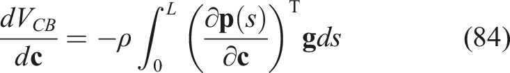
The derivative of the gravitational potential energy of the spacer disks: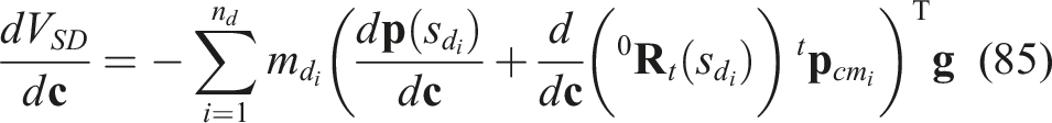
Combining the above terms, the ith row of the segment dynamics can be written as: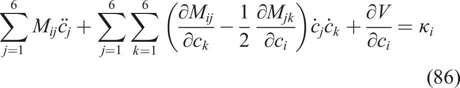
Using Christoffel symbols, the second term in the above equation can be written in terms of the centrifugal/Coriolis matrix, 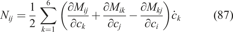
Supplemental Material
Supplemental Material
Footnotes
Declaration of conflicting interests
The author(s) declared no potential conflicts of interest with respect to the research, authorship, and/or publication of this article.
Funding
The author(s) disclosed receipt of the following financial support for the research, authorship, and/or publication of this article: This work was supported in part by the National Science Foundation grant #1734461 and by Vanderbilt University internal funds.
Supplemental Material
Supplemental material for this article is available online.
Notes
References
Supplementary Material
Please find the following supplemental material available below.
For Open Access articles published under a Creative Commons License, all supplemental material carries the same license as the article it is associated with.
For non-Open Access articles published, all supplemental material carries a non-exclusive license, and permission requests for re-use of supplemental material or any part of supplemental material shall be sent directly to the copyright owner as specified in the copyright notice associated with the article.