
Abstract
Robots will increasingly operate near humans that introduce uncertainties in the motion planning problem due to their complex nature. Optimization-based planners typically avoid humans through collision avoidance chance constraints. This allows the planner to optimize performance while guaranteeing probabilistic safety. However, existing real-time methods do not consider the actual probability of collision for the planned trajectory but rather its marginalization, that is, the independent collision probabilities for each planning step and/or dynamic obstacle, resulting in conservative trajectories. To address this issue, we introduce a novel real-time capable method termed Safe Horizon MPC that explicitly constrains the joint probability of collision with all obstacles over the duration of the motion plan. This is achieved by reformulating the chance-constrained planning problem using scenario optimization and predictive control. Out of sampled realizations of human motion, we identify which cases affect the optimization. This allows us to certify the planned trajectory in real-time. Our method is less conservative than state-of-the-art approaches, applicable to arbitrary probability distributions of the obstacles’ trajectories, computationally tractable and scalable. We demonstrate our proposed approach using a mobile robot and an autonomous vehicle in an environment shared with humans.
Keywords
1. Introduction
Mobile robots can improve our quality of life, from transporting goods in warehouses (Simon, 2019) to helping us commute more efficiently and safely using self-driving vehicles (Walker, 2019). In most applications where robots are currently deployed, the operating domain does not allow the robots to operate near humans or they do so in a conservative manner to simplify the robot navigation task. To deploy mobile robots in real-world environments, such as our cities, they need to be capable of navigating among humans, which remains challenging.
In crowded environments, the robot needs to understand and infer the motion of humans in order to move safely and efficiently. Unfortunately, human behavior is hard to predict and varies per person. In addition, human intentions cannot be explicitly communicated to the robot. This inherently makes the motion prediction of humans nondeterministic. Recent perception methods, such as Kooij et al. (2019), Salzmann et al. (2021), and Yue et al. (2023), infer human intentions, returning probabilistic information concerning humans. These probabilistic predictions need to be considered and exploited by the motion planner.
If we look at the motion planning problem from a probabilistic perspective, the occurrence of a collision is a probabilistic event. Our goal is to assess and bound the Collision Probability (CP) of the planned trajectory. This is challenging because of the non-Gaussian and multi-modal, that is, multiple paths are possible, distributions involved when predicting human behavior. In addition, when the collision probability spans a duration, for example, over the planned trajectory, then it must consider the correlation over time. The time correlation exists because the first collision in a trajectory renders it unsafe, such that all subsequent collisions can be ignored. Almost all of previous works, such as Blackmore et al. (2006), Luders et al. (2010), van Den Berg et al. (2011), Zhu and Alonso-Mora (2019), Wang et al. (2020a, b), and De Groot et al. (2021), do not account for this correlation, which leads to conservative trajectories. Similarly, the collision probability in these works is computed per obstacle, which degrades performance when more obstacles influence the plan, that is, in crowded environments. By accounting for the correlation in time and by considering all obstacles, one would be able to plan more efficient trajectories without compromising safety.
We achieve this goal by devising a novel probabilistic safe motion planner based on scenario optimization and nonlinear Model Predictive Control (MPC). Nonconvex scenario optimization (Campi et al., 2018) is a sampling-based approach for assessing the probability that a constraint holds under uncertainty. In the context of this paper, the imposed constraint probabilistically enforces collision avoidance between the controlled robot and the dynamic obstacles over the duration of the motion plan (see Figure 1). Scenario optimization has found limited applications in robotics. Its a posteriori safety verification is computationally demanding and it cannot directly be applied to distributions with unbounded support (e.g., Gaussians). We address these limitations in this work for our target application of motion planning in dynamic 2D environments, enabling its use in similar robotics applications. Overview of the proposed scenario-based motion planner. Predicted obstacle trajectories are sampled to obtain scenarios, where each scenario represents a trajectory for all obstacles over the planning horizon. By ensuring safety for all scenarios, probabilistic safety of the motion plan is guaranteed.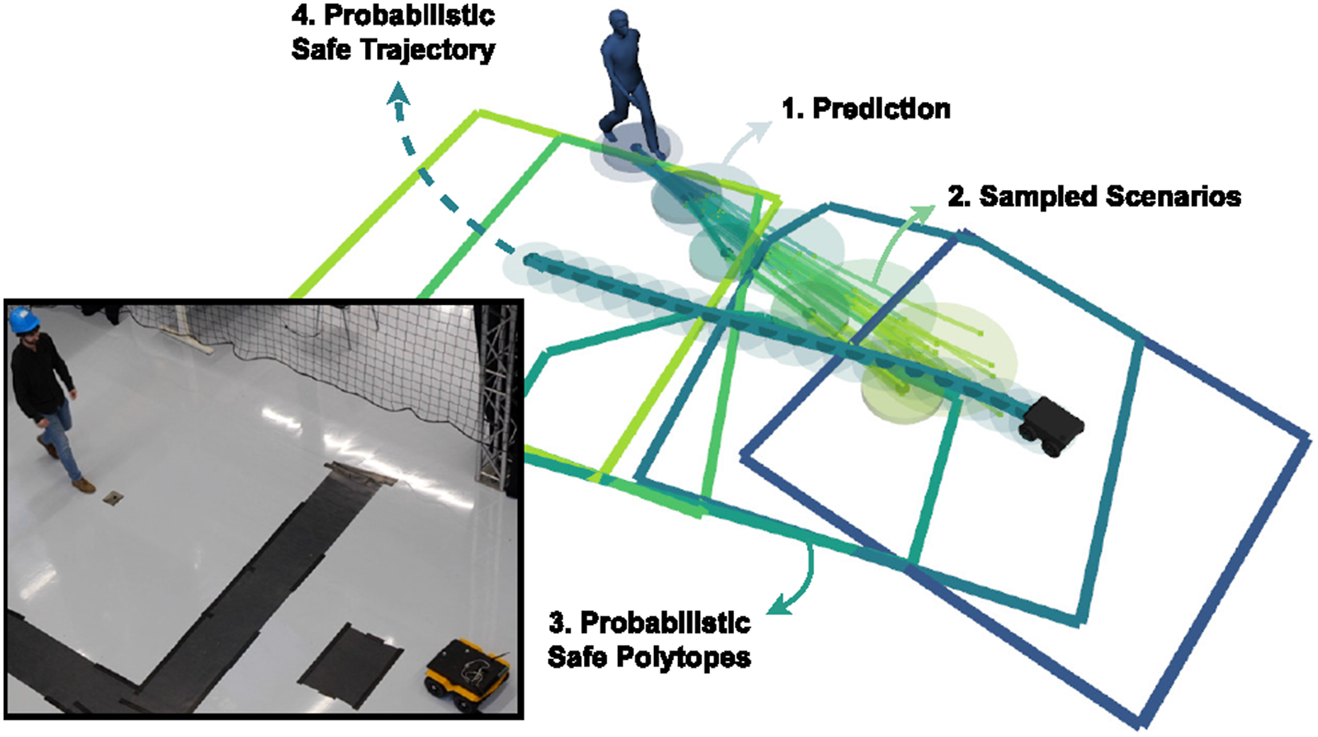
In practice, the uncertainty associated with the motion of detected obstacles is predicted forward in time (Step 1). We sample scenarios from these predictions that describe the trajectories of all dynamic obstacles during the planning horizon (Step 2) and construct collision avoidance constraints around each of the scenarios (Step 3). The robot trajectory is optimized with respect to the constraints (Step 4), which provides probabilistic collision avoidance. This is, to our knowledge, the first real-time capable method that bounds the CP of the planned trajectory jointly, in contrast with the existing state-of-the-art where the same quantity is conservatively approximated through its marginals. Our method therefore provides more consistent real-time guarantees on the CP, irrespective of the number of time steps and obstacles, and the underlying probability distribution that describes obstacle motion. This ultimately enables our method to trade-off safety and planning performance more accurately. We refer to our novel probabilistic safe motion planner as Safe Horizon MPC (SH-MPC).
2. Related work and contribution
A sizable body of literature exists on motion planning for safe, autonomous navigation. In this section, we review some of the existing work on trajectory optimization with collision avoidance under uncertainty. For a general overview of autonomous navigation, we refer the reader to Paden et al. (2016) and Schwarting et al. (2018b).
2.1. Collision avoidance under uncertainty
An important problem in autonomous navigation is to prevent collisions with dynamic obstacles. In trajectory optimization (Brito et al., 2019; Schwarting et al., 2018a), the navigation problem is formulated as an optimization problem where performance criteria are optimized (e.g., lane following and progress towards the goal) under constraints (e.g., collision avoidance and actuator limits). Due to large and multi-modal uncertainties in human motion prediction, collision avoidance in the mean or nominal case (e.g., constant velocity) may lead to collisions in practice. Many works therefore consider how to address this uncertainty.
One can consider the collision avoidance problem as a special case of optimization under uncertainty, for which two common approaches exist. Robust optimization (Ben-Tal and Nemirovski, 1998) requires the constraints to be satisfied for all possible realizations of the uncertainty, while stochastic optimization (see Mesbah (2016) for an overview) allows for a violation of the constraints, as long this happens with a probability smaller than an upper bound ϵ. Because the set of all possible realizations is often not available or too conservative, we focus in the remainder of this section on stochastic optimization. We refer to Kouvaritakis and Cannon (2016) for more details on both methods in the context of Model Predictive Control (MPC).
2.2. Collision-avoidance chance constraints
The probability of constraint violation in stochastic optimization is specified through chance constraints, which constrain the probability that a nominal constraint is satisfied. Exact evaluation of these chance constraints is however intractable in almost all applications. Existing works therefore focus on an approximation of the constraints. These can be divided into discrete-time and continuous-time methods. Discrete-time methods (e.g., Blackmore et al. (2006)) consider the CP at a fixed set of time intervals, usually at the discretization time of the robot dynamics. Continuous-time methods (e.g., Frey et al. (2020)) instead consider the CP over a continuous time interval, resulting in more accurate approximations but usually at a high computational cost. For our real-time application, we focus on the discrete-time methods. Existing discrete-time methods usually approximate chance constraints through additional assumptions on the probability distribution associated with the uncertainty, for example, by assuming Gaussian distributions in Zhu and Alonso-Mora (2019) and in Fisac et al. (2018) or through additional assumptions on the controlled robot, for example, by assuming linear dynamics in Blackmore et al. (2006). The recent works (Wang et al., 2020a; De Groot et al., 2021) have resolved many of the assumptions, making the framework applicable to nonlinear robot dynamics and arbitrary probability distributions. However, the chance constraints in these and many other works are not imposed on the robot’s planned trajectory, that is, the timed sequence of planned positions, but rather on each of its individual positions over the planning horizon. This fails to accurately bound the probability of colliding at any time. Similarly, chance constraints imposed per obstacle fail to estimate the probability of colliding with any obstacle. In this regard, three types of chance constraint formulations have been considered in previous work: Marginal, Conditional, and Joint.
2.2.1. Marginal chance constraints
Constraints on each position along the trajectory are referred to as marginal chance constraints. Let event A
k
denote the case that no collisions occur at time k and
Additive approaches impose constraints on each marginal probability (i.e.,
The multiplicative formulation explicitly constrains the product of the marginal probabilities. It was applied in van Den Berg et al. (2011) to plan motion under sensing and actuation uncertainty. An alternative marginal formulation is proposed in Fisac et al. (2018), which bounds the largest marginal constraint violation.
The limitation of marginal approaches is that the bound on the CP of the trajectory is inaccurate, as noted by Patil et al. (2012) and Janson et al. (2018). It is shown in Janson et al. (2018) that the trajectory CP approaches ∞ and 1 for the additive and multiplicative formulation, respectively, when the number of evaluations in the trajectory increases, regardless of the real CP. Marginal constraints only asses the risk correctly for the first time step and a single obstacle. The risk of the remainder is under- or overestimated. Overestimation of the risk and the associated unsafe space along the time horizon can cause the planning problem to become infeasible and may cause the robot to freeze. Due to these limitations, Patil et al. (2012) conditioned marginal chance constraints on being collision-free at prior times and evaluated them by truncating the part of the distribution in collision in each time instance. This formulation is more accurate but is limited to Gaussian distributions.
2.2.2. Joint chance constraint
Some authors formulate a joint chance constraint on the CP of the planned trajectory. Joint chance constraints estimate the open-loop risk over the time horizon more accurately, making it less likely that the problem becomes infeasible and improving performance. The joint CP can be evaluated by using sampling-based methods (Janson et al., 2018). In particular, Blackmore et al. (2010), Janson et al. (2018), and Schmerling and Pavone (2017) consider Importance Sampling Monte Carlo (ISMC) sampling to approximate the CP. An empirical estimate of the constraint violation is obtained by sampling the joint distribution over trajectories and evaluating the constraint for each sample. Since MC methods approximate the CP and its gradient with sampling, they can be computationally expensive to apply in trajectory optimization without further alterations. An alternative is to formulate a mixed-integer problem (Blackmore et al., 2010) to decide which samples may be violated, but these problems are hard to solve in real-time.
2.3. Scenario optimization
Rather than constraining each of the marginal CPs along the planned trajectory, we constrain the joint CP of the trajectory. We solve the resulting problem with Nonconvex Scenario Optimization (NSO) (Campi et al., 2018) under an explicit chance constraint on the joint CP. Scenario optimization is well established for convex optimization under uncertainty (Calafiore and Campi, 2006; Campi and Garatti, 2008, 2011; Schildbach et al., 2013) and has recently been extended to the general nonconvex case (Campi et al., 2018; Garatti and Campi, 2023). NSO solves the optimization problem under uncertainty by drawing a large set of samples from the uncertainty, that is, possible future motions of all obstacles, and formulating a deterministic constraint, for example, collision avoidance, for each sample. Our approach leverages a constraint formulation where many of the sampled constraints can be pruned, resulting in a deterministic program that can efficiently be solved online.
The NSO framework (Campi et al., 2018) cannot directly be applied to reformulate the joint collision avoidance chance constraint. To assess probabilistic safety, it traditionally needs to repeat the optimization problem once for each scenario and thus cannot be applied in real-time. In addition, unbounded distributions (e.g., Gaussian distributions) cannot be readily incorporated. We address these limitations in this work, including distributions with unbounded support (Sec. 5.1) and significantly reducing the computational complexity of the online safety assessment (Sec. 5.3) for our application to motion planning in dynamic environments. This allows us to apply the framework to online motion planning in real-time.
2.4. Contribution
The contributions of this paper are: (1) A novel trajectory optimization method, Safe Horizon MPC, that explicitly constrains the collision probability over the full duration of the planned trajectory. This distinguishes our work from previous work, where the collision probability is constrained per planning time instance. The idea is that each sample we draw from the distribution of the uncertain obstacle trajectories corresponds to a single collision avoidance constraint over the horizon. We want to stress that each sample represents a possible trajectory for all obstacles. The probability of collision is controlled through the number of samples drawn. By relying on sampling, our planner is distribution agnostic. (2) An approach that, under a convexity assumption on the iterations of the underlying optimization algorithm (that holds, for example, for Sequential Quadratic Programming), identifies the scenarios that hold the solution in place (known as the support) during optimization, in contrast with the general framework of Campi et al. (2018) where the support is computed after optimization. We leverage this information to certify the motion plan online.
We compare our approach in two simulation environments, on a mobile robot and a self-driving vehicle, with pedestrians against marginal baselines and show that our method achieves shorter task durations while maintaining the probabilistic safety specification. In addition, we show that the computation times scale well with respect to the number of obstacles and the type of distribution. Finally, we deploy our method on a mobile robot navigating among pedestrians. Our planner is implemented in C++/ROS and will be released open source.
2.5. Notation
Vectors and matrices are expressed in bold and capital bold notation, respectively. We use ⋀ to denote the “and” operation and ⋁ to denote the “or” operation. The notation
3. Problem formulation
We consider a controlled robot with nonlinear discrete-time dynamics

3.1. Chance constrained planning problem
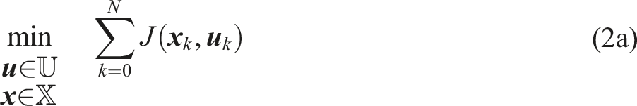
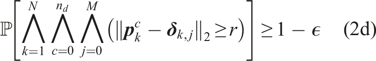
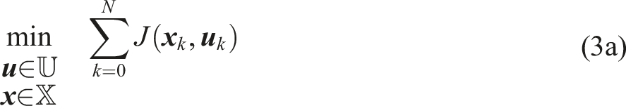
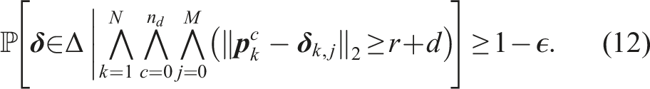
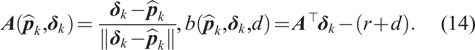
The planning problem is visualized in Figure 2. The dynamic uncertainty of other road users affects the navigation envelope of the robot. To constrain the probability of a collision with any obstacle along the horizon, we formulate a single chance constraint for collision avoidance. This leads to the following Chance Constrained Problem (CCP) The chance constrained motion planning problem considered in this paper with the robot (yellow) navigating under probabilistic motion predictions of obstacles (blue/green). The distribution of the motion predictions can take any form but is visualized here with several modes and their variance (arrows/shaded regions).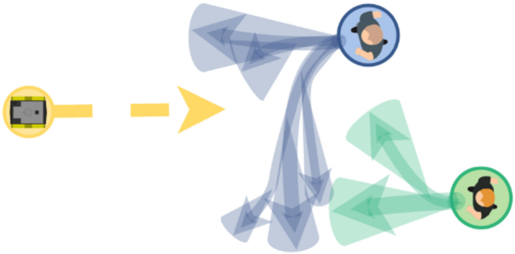
When


3.2. Scenario-based planning problem
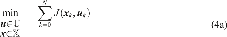
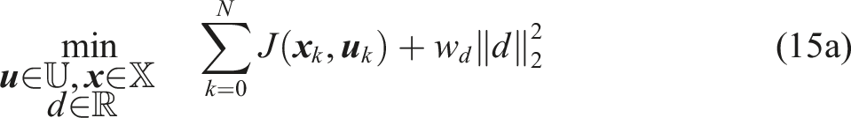
Directly evaluating chance constraint (2d) is not computationally feasible in closed loop. Our goal is to formulate a sampled deterministic version of the CCP, known as a Scenario Program (SP) (Campi et al., 2018). The challenges for safe robot navigation within this framework are to determine the number of samples that must be drawn and, consequently, to identify the samples that affect the optimization.
3.3. Paper organization
In the following, we first consider a more general CCP formulation that can be solved by the proposed framework. We provide a brief summary of the nonconvex scenario optimization framework of Campi et al. (2018) to show how this general class of CCPs can be solved via its associated SP. We then present our main results in Sec. 5, which shows how this SP can be solved in closed loop as MPC. Finally, we apply our main results to probabilistic motion planning in dynamic environments, in Sec. 6.
4. Nonconvex scenario optimization
In the following, we summarize the main results of the NSO framework of Campi et al. (2018) that we use to build our motion planning framework. To this end, consider the following generalization of Problem 1,
The nominal constraint g(


General SP.


We focus our attention on the planning problem by considering only finite sample sizes S. Assumption 1 is not trivially satisfied for motion planning. It requires that a feasible trajectory exists for all possible extractions in the support, which is particularly problematic for unbounded distributions (e.g., Gaussians). We will consider a relaxed constraint formulation in Sec. 5.1 to address this limitation. Since the scenario decision accounts for all sampled scenarios, each additional scenario makes the scenario decision more robust. Consequently, the more scenarios that are used to compute the scenario decision, the lower is the probability that the resulting decision will violate the constraints. Formally, the violation probability, V : Θ → [0, 1], given by


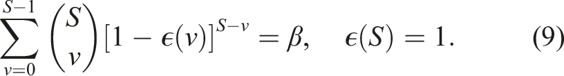
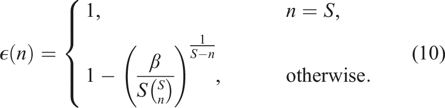
The cardinality of the support subsample is referred to as the support size, that is, The support size captures the number of scenarios necessary to hold the solution of the SP in place and is strongly correlated with its risk. This correlation can be used to derive a probabilistic guarantee on the solution of the SP using only the support and sample size. For a confidence 1 − β, Theorem 1 in Campi et al. (2018) provides the bound A general algorithm to determine the support is the greedy algorithm of Campi et al. (2018). After solving Problem 3, this algorithm removes one scenario at a time, solving Problem 3 again. If the solution changes for a scenario, then that scenario is part of the support. The samples remaining after checking all scenarios constitute a support subsample.


4.1. Limitations of NSO for motion planning
An SP can be constructed from the CCP in Problem 1 by sampling scenarios from the distribution over obstacle trajectories and formulating collision avoidance constraints for each scenario. However, this strategy is not directly applicable for the motion planning problem because of two limitations.
Our goal is to address these limitations so that we can solve Problem 1 with an SP to bound the joint CP.
5. Safe horizon model predictive control
This section introduces our safe motion planning framework. First, we reformulate the SP to obtain a real-time solvable problem that satisfies Assumption 1. Then, we show how the support can be estimated during optimization. Finally, we derive the sample size of the SP.
5.1. Motion planning scenario program
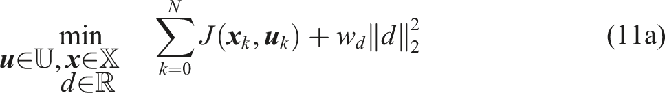
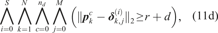
Safe Horizon MPC bounds the joint CP by solving an SP. In the planning problem, the scenarios extracted from Schematic illustration of Safe Horizon MPC applied to a mobile robot. (a) Scenarios are sampled from the trajectory distributions. Each time instance of SP (Equation (4)) is associated with a set of sampled obstacle positions as visualized by the green and blue circled pedestrians. (b) Halfspace constraints are constructed between sampled obstacles and the robot, and are reduced to a probabilistic safe polytope for each time instance and robot disc, depicted by the yellow lines. (c) Problem 5 is solved via Algorithm 1. The resulting trajectory is certified up to a probabilistic bound.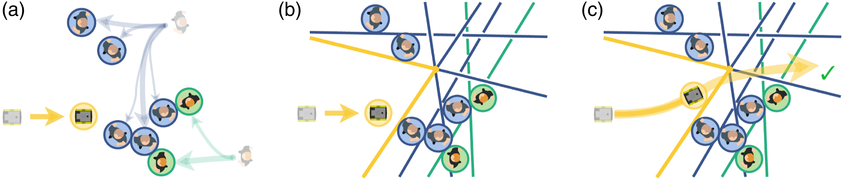


5.2. Improved computational efficiency
While Problem 4 can be solved with off-the-shelf nonlinear program solvers, its problem statement is computationally inefficient. The collision-free space described by (11d) is nonconvex and can lead to high support (i.e., requiring many samples). We consider a more efficient overapproximation of the collision avoidance constraints with lower support.
We linearize the collision regions with respect to the previously planned robot trajectory (denoted


The linearization exploits the geometry of the motion planning problem to reduce the size of the support. Most of the linearized constraints become redundant (they are fully contained in other constraints) and can be excluded from the planning problem. We provide more details in Appendix A.
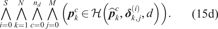
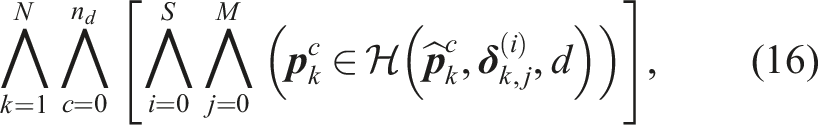
To drastically reduce the computational demand of this formulation, we reorder Constraints (15d) as
The final SP that is solved online, after pruning, is given by
The SH-MPC problem can be solved in real-time while bounding the joint CP of its trajectory (see Figure 3(c)).


5.3. Estimating the support
The joint CP that is bounded by SH-MPC depends on the sample size S and the support n. In the following, we propose an estimate of the support
For a convex SP, the support can easily be computed as its support constraints are active (Campi and Garatti, 2008; Garatti and Campi, 2019). Computing the support in the nonconvex case is much harder as this property does not hold. We show here that the support can be estimated through the active constraints after each iteration of the nonconvex optimization. An iteration refers to the procedure that is repeated to solve the nonconvex optimization, such that the decision algorithm can be described by a repeated sequence of iterations

The support set obtained through Lemma 1 is an overestimation. It is possible that a scenario changes the solution of an intermediate iteration without changing the final solution. To apply this lemma to SH-MPC, we note that a local optimum of Problem 5 can be computed by iteratively linearizing the problem and solving a convex optimization. In this case, each iteration of the solver is a convex scenario optimization for which the support constraints are active (Campi and Garatti, 2008). For example, in Sequential Quadratic Programming (SQP), each iteration


The active constraints can be identified by verifying which of the scenario constraints of the convex program are exactly satisfied. We therefore require the additional assumption that the constraints of the convex problem are satisfied in each iteration.
The scenario constraints are in general nonlinear due to the robot dynamics. In each iteration, and as commonly done to solve nonlinear problems, the solver makes the problem convex, deriving constraints from the locally linearized dynamics. We only require that these constraints are satisfied. Using these assumptions, we propose the following support estimation.
The support of SH-MPC can therefore be estimated by the aggregated set of active scenarios over all iterations, addressing Limitation 2. In practice, we use Sequential Quadratic Programming (SQP) (Nocedal and Wright, 2006) Chapter 18 to solve Problem 5, which satisfies Assumption 2 (convexity of iterates) and Assumption 3 (feasibility of intermediate iterates).

5.4. Determining the sample size
With the support of SH-MPC estimated through Theorem 1 and directly available after optimization, it remains to determine the sample size S for SH-MPC such that the joint CP of its trajectory is at most ϵ.
Problem 5 can only be solved once due to the strict real-time requirements on the planner. We therefore propose to find a sufficiently high S that certifies the joint CP almost always. To that end, we define a support limit
Theorem 2 shows that SH-MPC solves the CCP in Problem 1 if its support is lower than the support limit (and if d = 0). In practice, the support limit can be estimated by deploying the planner and collecting the support estimation of Theorem 1. In our approach, we keep track of the largest estimated support over a large number of iterations and use this empirical worst-case support as the support limit. An alternative could be to start with a large support limit, lowering it when it is not passed for many iterations. Since the support limit is likely higher than necessary for many iterations, the trajectories computed by SH-MPC become conservative. The support limit however allows the planner to incorporate the joint collision avoidance chance constraint in real-time. Conservatism can be reduced by running several instances of SH-MPC in parallel (along the lines of Mustafa et al. (2023)), which can lead to lower and more consistent support. Alternatively, the support limit could be continuously adapted based on its online estimation. We consider these future work.
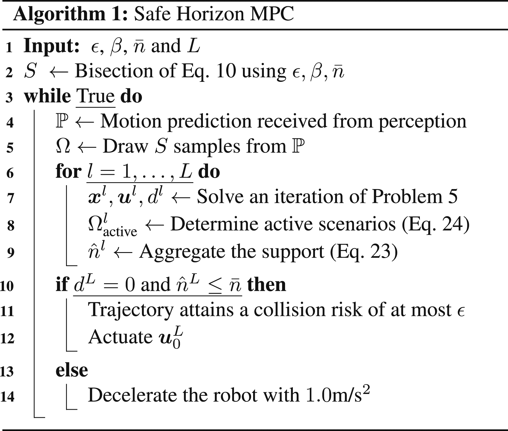
5.5. Algorithm outline
Algorithm 1 summarizes the SH-MPC framework. Offline, we compute the sample size S based on the joint CP ϵ, confidence 1 − β and support limit
6. Results
We evaluate SH-MPC in simulation, comparing against two MPC baselines, and in real-world experiments on a mobile robot among pedestrians. A video of the results accompanies this paper (De Groot et al., 2024a).
6.1. Simulation setup
We consider a mobile robot moving through an environment with pedestrians (see Figure 4) in which the robot is modeled by a kinematic unicycle model (Siegwart and Nourbakhsh, 2011). We assume throughout that the distribution of pedestrian motion is known in order to evaluate the performance of the planner in isolation (i.e., without prediction errors). We first validate on a Gaussian case, where the baselines may leverage the shape of the distribution to approximate the probabilistic collision-free space accurately. In this case, the pedestrian dynamics are given by Planned trajectories for the different methods in the Gaussian simulation with eight pedestrians. The robot plan and associated collision areas are drawn in blue. For all methods, visualizations are shown in blue to green colors for stages 0, 5, 10, 15, and 19, respectively. (a) Circles show the predicted areas occupied by the obstacles following the mean of the Gaussian distribution. (b) Circles show the level sets of the Gaussian distribution at the specified ϵ. (c) Sampled pedestrian positions (excluding pruned samples in the center) are drawn as points with their collision area, borders of the safe polytopes are drawn as colored lines. (d) Similar to (c) but depicting sampled trajectories as dashed lines and highlighting support constraints. (a) Deterministic baseline. (b) Gaussian baseline at ϵ
k
= 0.0003125. (c) S-MPCC at ϵ
k
= 0.0025. (d) SH-MPC at ϵ = 0.05.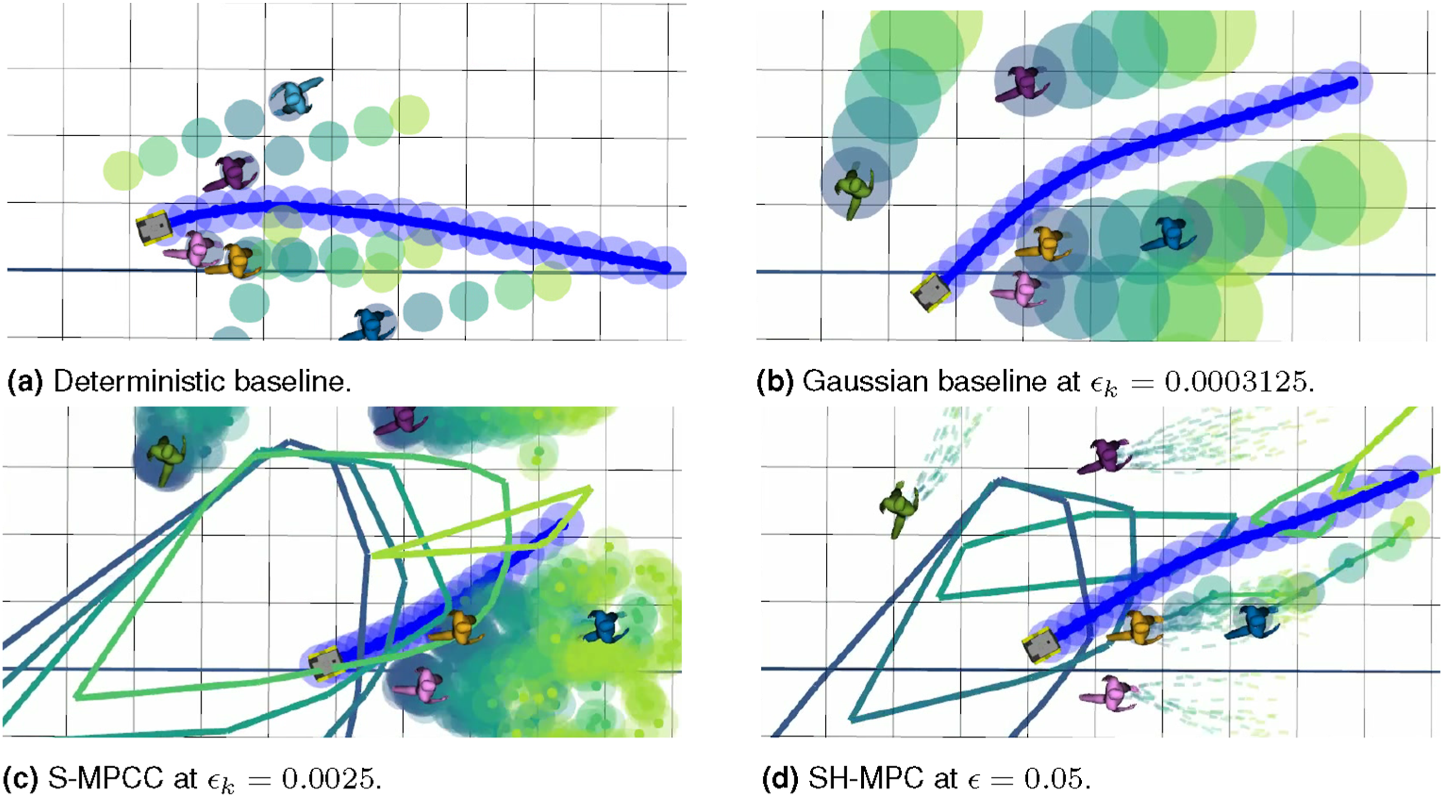

6.2. Implementation of SH-MPC
All baselines and SH-MPC use the Model Predictive Contouring Control formulation in Brito et al. (2019), which tracks a reference path and reference velocity while penalizing robot inputs. We solve Problem 5 using the Forces Pro SQP solver (Domahidi and Jerez, 2014) with at most 12 iterations. We empirically selected the support limit
6.3. Baselines
We compare SH-MPC against a deterministic baseline and two probabilistic baselines that constrain the marginal CP, that is, the independent CP per time instance and/or obstacle. (1) (2) (3)
S-MPCC handles arbitrary distributions. It solves an SP where scenario constraints are posed on the marginal distributions. For each time k, it samples from the independent obstacle distribution at k to obtain a collision-free polygon. It is assumed that all constraints in the polygon are of support (set to 20 in these simulations), which requires S = 75946 for instance when ϵ k = 0.0025. Samples in the center of the distribution are pruned in the Gaussian case to reduce the number of samples considered online.
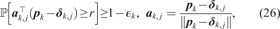
CC-MPC is strictly applicable to Gaussian distributions. It approximates the collision probability via the Cumulative Density Function (CDF) of the Gaussian distribution. The linearized collision avoidance chance constraint

Since SH-MPC is characterized by a single bound ϵ on the trajectory CP, while the baselines specify bounds ϵ k on the CP for each k and for each obstacle, we consider three versions of the baselines. The first sets ϵ k = ϵ, which is not provably safe but relies on updates of the controller to remain safe. The second version sets ϵ k = ϵ/N, accounting for the marginal approximation over time since ∑ k ϵ k = ϵ, but ignoring marginalization per obstacle. As S-MPCC inherently accounts for the obstacle marginalization, it matches SH-MPC’s safety specification (joint CP of ϵ) with this version. The third version accounts for both marginalizations, setting ϵ k = ϵ/NM such that M∑ k ϵ k = ϵ. CC-MPC only attains the same safety specification as SH-MPC using this last version.
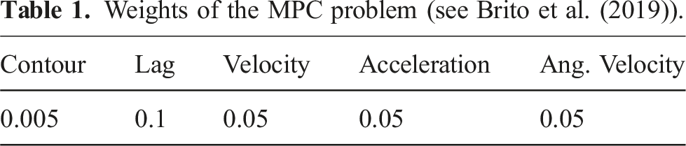
6.4. Weights and parameters
Weights of the MPC problem (see Brito et al. (2019)).
6.5. Baseline comparison—Gaussian uncertainties
We consider an environment with multiple dynamic pedestrians following the dynamics in equation (25) where
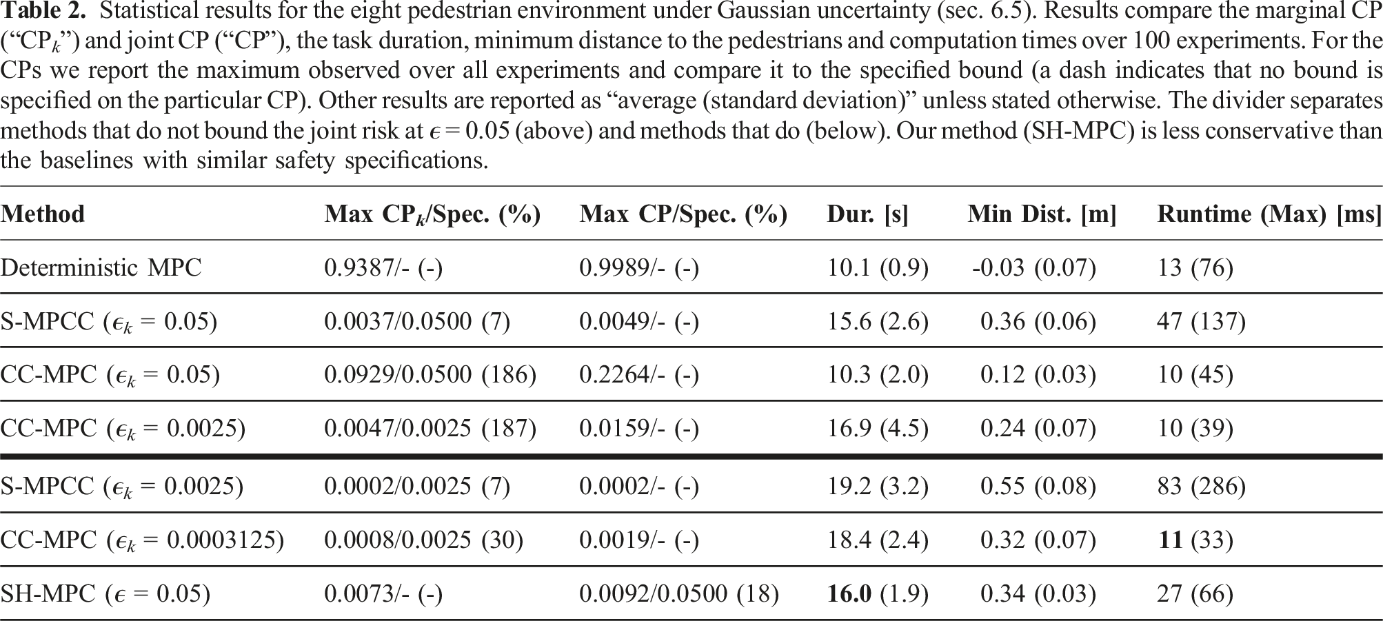
Statistical results for the eight pedestrian environment under Gaussian uncertainty (sec. 6.5). Results compare the marginal CP (“CP k ”) and joint CP (“CP”), the task duration, minimum distance to the pedestrians and computation times over 100 experiments. For the CPs we report the maximum observed over all experiments and compare it to the specified bound (a dash indicates that no bound is specified on the particular CP). Other results are reported as “average (standard deviation)” unless stated otherwise. The divider separates methods that do not bound the joint risk at ϵ = 0.05 (above) and methods that do (below). Our method (SH-MPC) is less conservative than the baselines with similar safety specifications.
6.6. Baseline comparison: Gaussian mixture
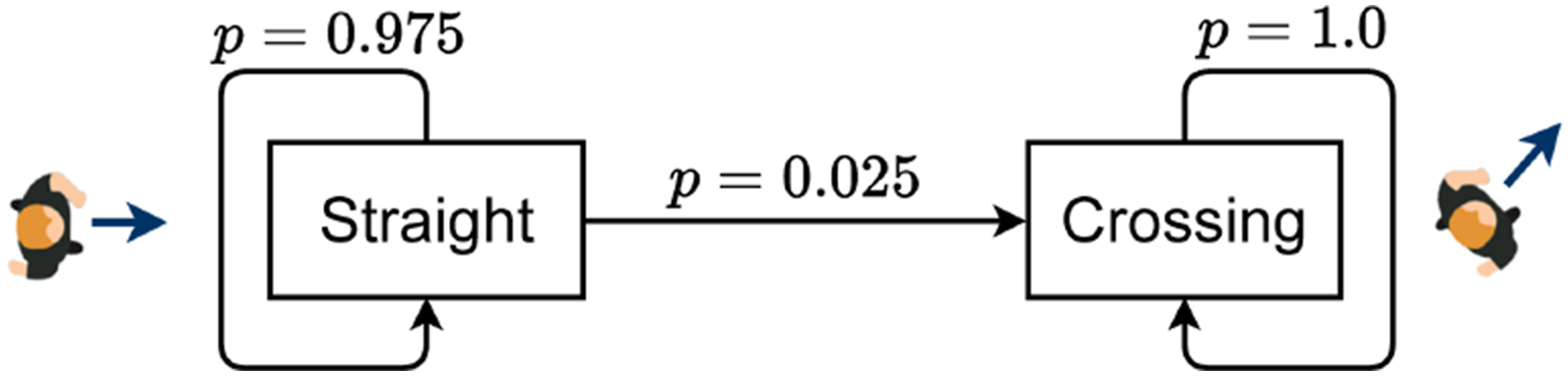
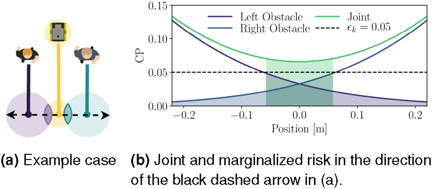
We now modify the distribution to incorporate a probability that the pedestrians will cross. We encode this scenario with a Markov Chain (see Figure 5) that changes pedestrian movement from horizontal to diagonal in addition to the Gaussian process noise of the previous simulations. We define the pedestrian dynamics as Markov chain modeling of a crossing pedestrian. A 1D illustration of the case where two obstacles constrain the robot. Even though the marginal probability of collision for each obstacle is less than ϵ
k
(shaded tails) in the center region, the joint probability of collision in the feasible region (green shaded area) is larger than ϵ
k
. (a) Example case. (b) Joint and marginalized risk in the direction of the black dashed arrow in (a).
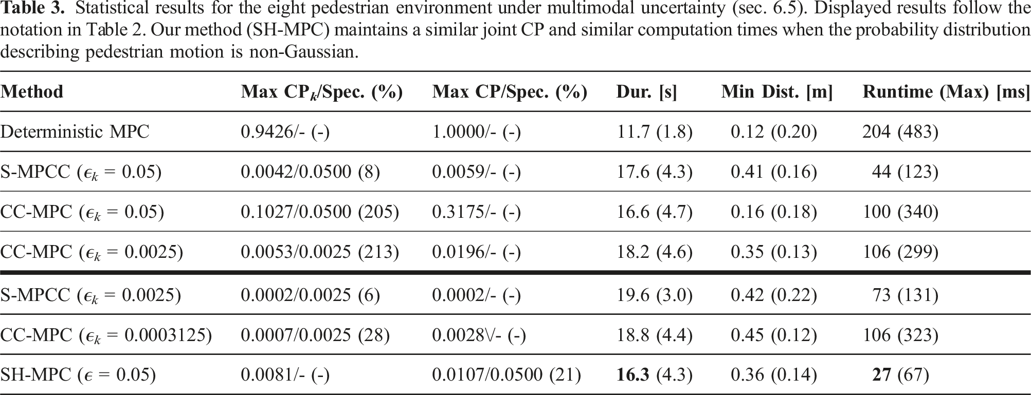
Statistical results for the eight pedestrian environment under multimodal uncertainty (sec. 6.5). Displayed results follow the notation in Table 2. Our method (SH-MPC) maintains a similar joint CP and similar computation times when the probability distribution describing pedestrian motion is non-Gaussian.
6.7. Empirical analysis and sensitivity
6.7.1. Support estimation
We compare our proposed support estimation in equation (23) with the default Greedy algorithm of Campi et al. (2018) in a scenario with one static pedestrian. We manually vary the sample size between 100 and 1000 and collect, for 100 iterations of each sample size, the runtime of the optimization with support estimation and the estimated support size. Figure 7 shows that, while the runtime of our support estimation is negligible compared to the optimization, the greedy algorithm takes roughly S + 1 times as long to solve. The mean and standard deviation of the runtime (top) and estimated support size (bottom).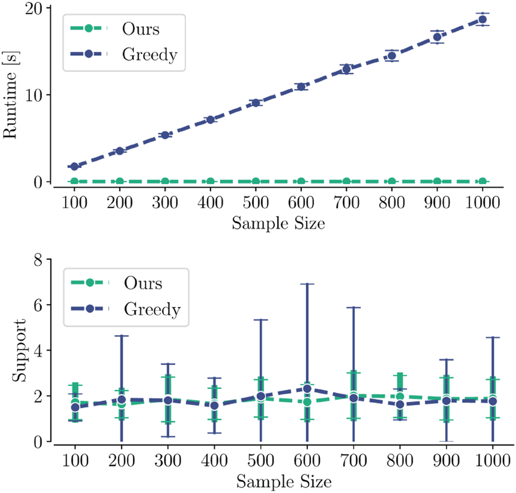
6.7.2. Empirical risk distribution
We visualize the empirical distribution of the joint CP for each value of the support estimate in Figure 8 computed for the simulations of Sec. 6.5. In line with the theory, we observe that the trajectory CP is on average higher for higher support values. Our support limit (n = 10) is reached in only 2 out of 33564 cases and is never exceeded. In the other cases, our support limit is conservative. In the simulations of Sec. 6.6, the support limit is exceeded six times in total. This usually indicates that the planner’s intended trajectory is becoming increasingly risky and is a valid cause for slowing the robot down. The same situation can result in d > 0 (i.e., infeasible optimization problem) of which we detected 50 occurrences in the same simulations. The empirical distribution of the joint CP for SH-MPC for each estimated support over 33,564 planner iterations (in simulations of Sec. 6.5). Dots denote individual planner iterations. Boxplots denote the statistics per support value.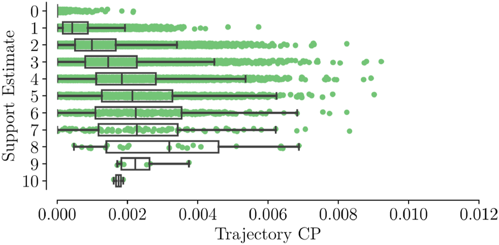
6.7.3. Sensitivity to ϵ and N
We validate the sensitivity of SH-MPC to varying risk specifications (ϵ) and horizon lengths (N) in the scenario of Sec. 6.5. Figure 9(a) shows that reducing the specified risk results in longer task durations and that the approach becomes slightly more conservative for lower risk specifications. In line with the theory, Figure 9(b) indicates that changing the horizon length does not significantly affect the CP. Instead, the trajectories become more cautious when the same risk must be guaranteed over a longer duration. Sensitivities of the empirical CP and task duration with respect to (a) the specified CP with constant N = 20 and (b) the horizon length with constant specified CP ϵ = 0.05, evaluated over 25 experiments in the setting of Sec. 6.5. (a) Risk sensitivity. (b) Horizon sensitivity.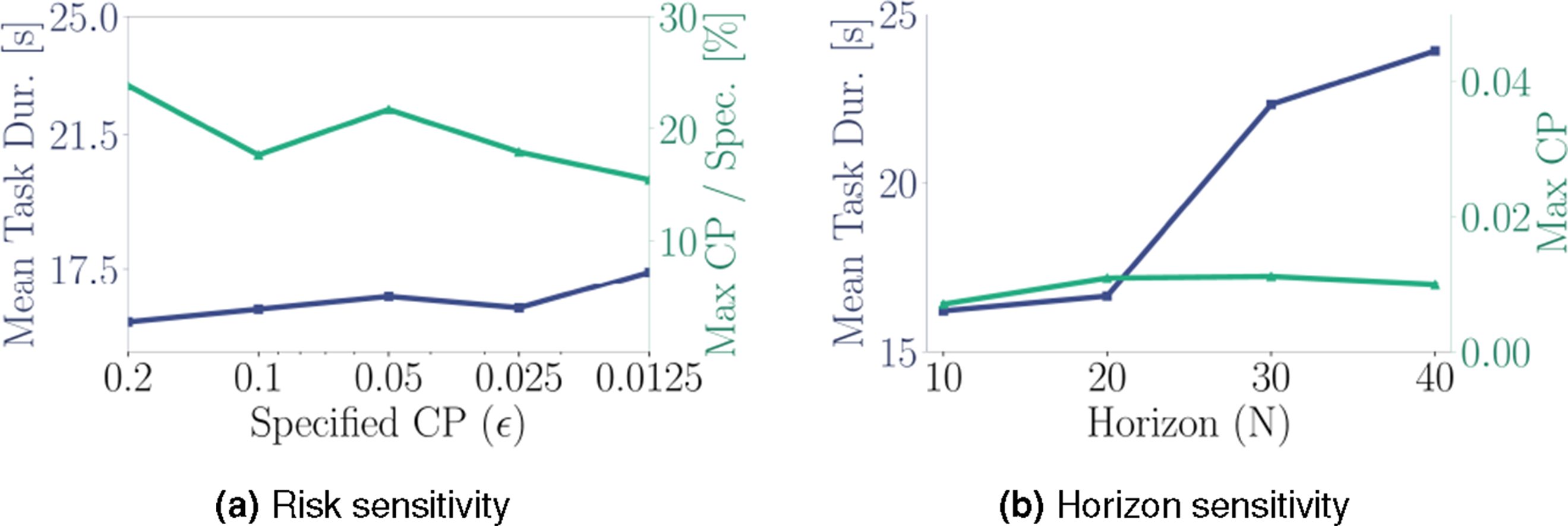
6.8. Real-world experiments
We validate SH-MPC in the real world by applying the planner on a mobile robot navigating among pedestrians. The experimental setup consists of a Clearpath Jackal and up to three pedestrians in a 7 m × 9 m space. We detect the positions of all agents with a motion capture system. The robot is given a reference path along the center of the space and a reference velocity of 1.5 m/s. When the robot reaches the end of the reference path, it rotates without MPC control and is given the reversed reference path. The robot is controlled at 20 Hz by SH-MPC that models the dynamics as a second-order unicycle. We specify an acceptable risk of ϵ = 0.05 over a 20 step and 4s horizon with confidence 1 − β = 0.99 and support limit
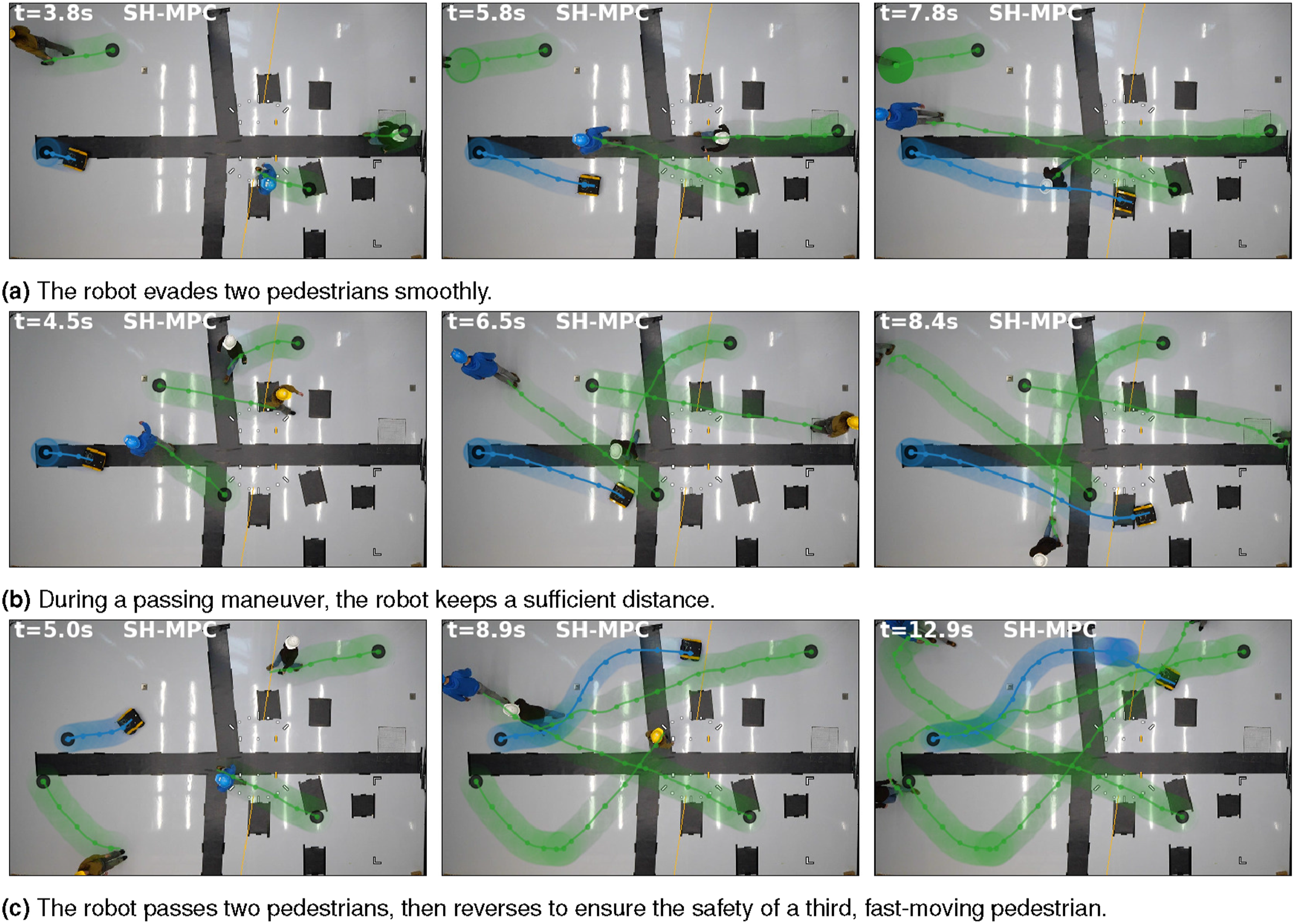
Figure 10 depicts three experiments with one pedestrian. SH-MPC keeps its distance from the pedestrian so that its motion remains smooth even when the pedestrian deviates from constant velocity behavior. In Figure 10(a) and 10(b), it keeps sufficient lateral distance when passing, while in Figure 10(c), it reacts to the pedestrian speeding up its pace. Figure 11 shows three experiments with three pedestrians. The robot evades the pedestrians smoothly in this more crowded environment. In Figure 11(a) and 11(b), the robot smoothly evades multiple pedestrians. In Figure 11(c), the planner first evades two pedestrians, then reverses to ensure the safety of the third, fast-moving pedestrian. Past trajectories of the robot and one pedestrian overlayed with top-view camera images. By accounting for the possible future motion of the pedestrian, SH-MPC remains safe and smooth even when the pedestrian deviates from constant velocity behavior. (a) The pedestrian turns in a straight encounter. (b) The pedestrian turns with the robot passing from behind. (c) The pedestrian speeds up. Past trajectories of the robot and three pedestrians overlayed with top-view camera images. The robot consistently avoids collisions with pedestrians. (a) The robot evades two pedestrians smoothly. (b) During a passing maneuver, the robot keeps a sufficient distance. (c) The robot passes two pedestrians, then reverses to ensure the safety of a third, fast-moving pedestrian.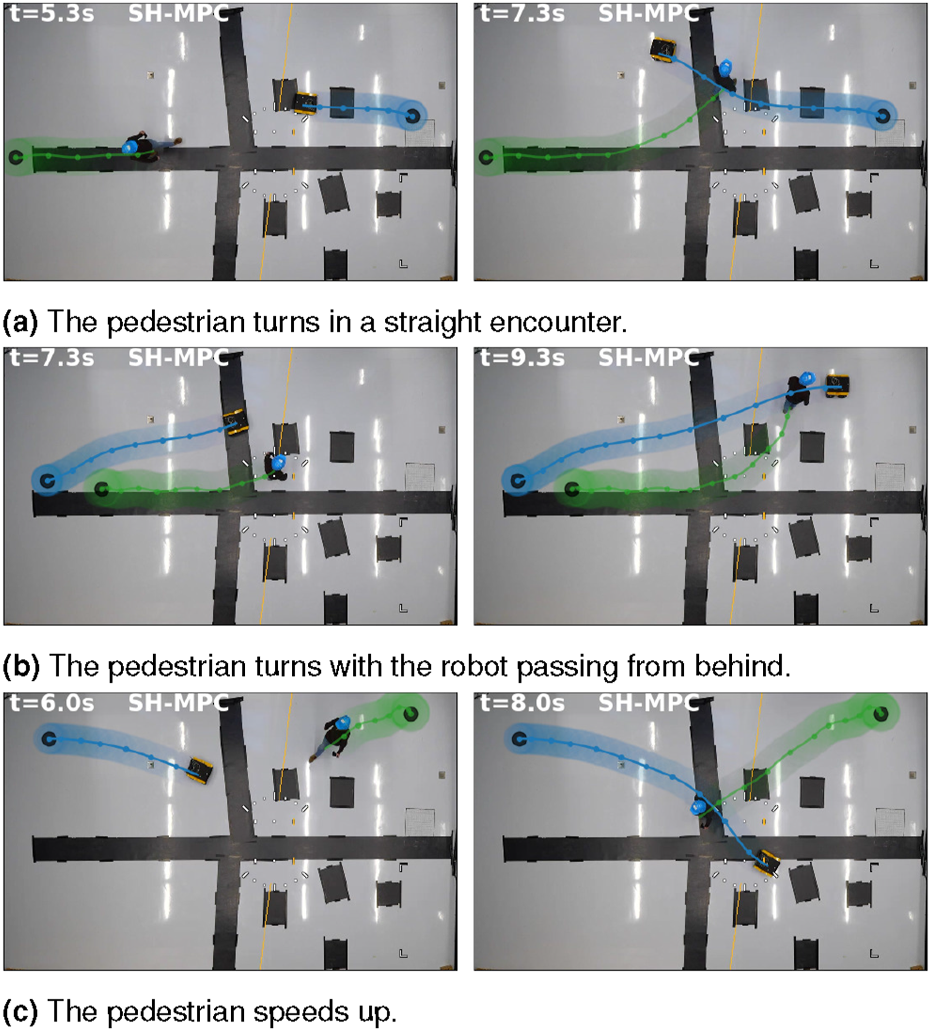
With 1 pedestrian, the support limit was never exceeded. With three pedestrians, it was exceeded 30 times in total. This could be resolved by increasing the support limit when it is exceeded. In our case, slowing down led to safe behavior. We did not observe collisions in any of the experiments. Because the proposed planner is a local planner, it does sometimes get infeasible when its intended passing maneuver becomes impossible within the specified risk. This can be resolved by considering multiple distinct maneuvers in parallel (e.g., as considered in De Groot et al. (2023)) but this is outside of the scope of this paper.
6.9. Autonomous navigation in an urban environment
SH-MPC can be applied to different robot morphologies and scenarios. To demonstrate this, we deploy our approach on a simulated self-driving vehicle in Carla simulator (Dosovitskiy et al., 2017). The dynamics are modeled with a second-order bicycle model (Kong et al., 2015) and the collision region consists of three discs. We construct a collision-free polytope for each of the discs. The pedestrians are programmed to follow the same dynamics as in Sec. 6.6, that is, a GMM modeling crossing behavior. We do not model the interaction between the vehicle and the pedestrians. The control frequency is 10 Hz. We measured the computation time to be 88 ms on average and 135 ms maximum. Figure 12 visualizes snapshots of the simulations. In Case A (see Figure 12(b)), the planner keeps enough distance to let the pedestrians cross while driving as close to the path as is safe. In Case B (see Figure 12(c)), the vehicle passes behind the pedestrians while keeping its distance from the pedestrian that is not crossing. (a) Snapshot from Carla simulations. Visualization follows Figure 4(d) for the frontal vehicle disc. (b, c) Observed trajectories of the vehicle (dark blue) and pedestrians (green) with start positions as black dots in two cases. (a) A snapshot of the proposed approach in the Carla simulator. (b) Case A: Safe overtake. (c) Case B: Passing behind.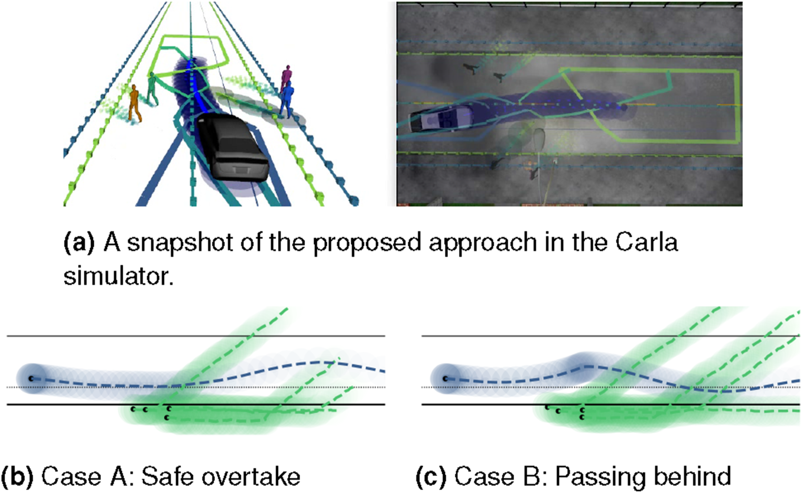
7. Discussion
As expected from the theoretical analysis, our experiments showed that SH-MPC can consistently bound the CP of the overall trajectory. Where methods that impose marginal constraints need to decide between performance (ϵ k = ϵ) and safety (ϵ k = ϵ/NM), SH-MPC makes this trade-off more explicit by ensuring that the CP remains consistent under different operating conditions, such as with regards to number of obstacles, probability distributions, and the horizon length.
The proposed method is widely applicable. It handles dynamic obstacles (e.g., cyclists, cars, or non-cooperative robots) and controls systems with nonlinear dynamics. In addition, the joint distribution of the uncertainty can capture interactions of dynamic obstacles with other obstacles or the robot (e.g., to predict that pedestrians evade other pedestrians and the vehicle). It cannot yet account for interaction during planning, where the dynamics of the robot and pedestrians directly influence each other, as the probability measure
7.1. Reducing conservatism
Planning performance could be improved by reducing the gap between the guaranteed and obtained risk, for example, by assuming some knowledge of the distribution or by running multiple scenario programs in parallel as considered in Mustafa et al. (2023). Over-approximating Monte Carlo sampling may be less conservative than NSO and may reduce conservatism while maintaining safety. Recent work (Brudermüller et al., 2024) proposed such an approximation. Their method is less conservative, but also computationally more demanding than SH-MPC, achieving about an order of magnitude slower computation times than SH-MPC without considering non-holonomic constraints.
The guarantees provided in this paper rely on an accurate model of the uncertainty, which may be challenging to obtain, for example, in the case of human motion prediction. Nevertheless, the proposed method provides a planner that attains a desired level of risk with respect to the predicted probability distribution. The prediction model could also be replaced by recorded samples (see De Groot et al. (2024b)), in line with the typical scenario approach, to reduce modeling errors and provide formal guarantees with respect to the true motion of the obstacles.
7.2. Computational efficiency
We showed that our approach is online capable and scalable under typical operating conditions. For extremely low risk specifications (e.g., ϵ ≤ 5 ⋅ 10−3), computational requirements may become excessive as a result of the increase in sample size. This can be addressed, for example, by either pruning the samples, given that only the extreme samples are of interest (see, for example, De Groot et al. (2021)), or by solving an approximate scenario optimization (Sartipizadeh and Açikmeşe, 2020). In addition, most computations of SH-MPC are parallel linear computations (for each sample), which potentially leave room for further optimization, for example, by delegating computations to a Graphical Processing Unit (GPU).
The computational efficiency of our approach derives from the merging of linear constraints which is facilitated by modeling collision regions as discs. While this modeling can be used to represent several obstacles, we currently cannot efficiently handle more complex shaped obstacles, such as objects with sharp corners. Future work could explore if other linear constraints (e.g., towards vertices of obstacles) could be merged safely. The same comment holds for extension to planning problems in higher dimensions. Directly merging halfspaces in 3D may, for example, be more complicated than in the 2D case and may require constraints of different shapes to be merged effectively.
7.3. Support limit
We showed that the support limit could be estimated online by using a solver that convexifies the problem in each iteration, such as SQP. Although this limits the generality of the support estimation, SQP solvers are a common choice for robotics applications. SH-MPC furthermore requires the user to estimate a support limit online because the support depends on the complexity of the problem to be solved. We do provide the online estimation of this single parameter, so that the user can bound it conservatively based on real-world data, enabling real-world robotics applications. Future work could explore if the support limit could be known before optimization. For example, by adapting the constraint formulation so that the support is fixed by construction (see Appendix A in Campi et al. (2018)).
8. Conclusions
Safe Horizon Model Predictive Control (SH-MPC) enabled mobile robots to constrain the joint open-loop probability of collision over the planned trajectory and with respect to all obstacles in real-time for 2D dynamic environments. It does so without making simplifying assumptions on the robot dynamics or underlying probability distribution describing the motion of the obstacles. The method uses a scenario optimization formulation where samples of the involved uncertainty are used as constraints to limit the collision probability of the motion plan. The number of samples is the main indicator for the collision probability and, under our approach, could be computed before deploying the controller.
Our results, with a mobile robot and an autonomous vehicle, showed that SH-MPC better approximates the collision probability over the duration of the motion plan than existing methods that rely on the marginal probability of collision. The main baseline, which achieved tight evaluations of the risk for each time step, was shown to be conservative over the duration of its motion plan and there was significant variation in its overall risk when we varied the underlying distribution. The overall risk of SH-MPC remained less conservative and more consistent between different environments and distributions, which resulted in faster trajectories. In addition, we showed excellent scaling of the computation time with respect to the number of obstacles and under varying distributions.
The real-time performance of SH-MPC is currently tied to a 2D environment with disc-shaped collision regions, while the probabilistic safety certification poses assumptions on the solver (satisfied by SQP) and requires the support limit to be estimated online. Our future work will try to alleviate these assumptions to further generalize our approach.
Supplemental Material
Footnotes
Acknowledgments
The authors would like to thank Bruno Brito for assisting in the simulated experiments.
Declaration of conflicting interests
The author(s) declared no potential conflicts of interest with respect to the research, authorship, and/or publication of this article.
Funding
This work received support from the Dutch Science Foundation NWO-TTW, within the SafeVRU project (14667) and Veni project HARMONIA (18165), and the European Union, within the ERC Starting Grant INTERACT (101041863). Views and opinions expressed are however those of the author(s) only and do not necessarily reflect those of the European Union or the European Research Council Executive Agency. Neither the European Union nor the granting authority can be held responsible for them.
Supplemental Material
Supplemental material for this article is available online.
Note
Appendix
In practice, linearization of the collision avoidance constraints results in a support that consists of a small subset of the scenarios. To support this observation, we consider here how the constraint formulation impacts the support.
An example shadow is visualized in Figure 13(a) for the proposed constraints. Note that in Figure 13(b), the shadow always occupies a non-zero area. This is a result of the linearization and a set of box constraints on the position that limit the range in which constraints are considered. In this case we can prove the following.
Although this does not prove that the support is bounded for finite S, it shows that it is very likely that redundant scenarios are sampled, which are not of support.
References
Supplementary Material
Please find the following supplemental material available below.
For Open Access articles published under a Creative Commons License, all supplemental material carries the same license as the article it is associated with.
For non-Open Access articles published, all supplemental material carries a non-exclusive license, and permission requests for re-use of supplemental material or any part of supplemental material shall be sent directly to the copyright owner as specified in the copyright notice associated with the article.