Nonlinear model predictive dynamic positioning of a remotely operated vehicle with wave disturbance preview

Abstract

Exploiting preview information of disturbances within robot control is an effective method of handling state perturbations. For underwater vehicles operating in wave-dominated environments, disturbances significantly influence vehicle response and pose a threat to operational safety. In consideration of this, a complete end-to-end control architecture is developed in this work for disturbance rejection during station keeping tasks under wave perturbations, encompassing a nonlinear model predictive controller (NMPC) combined with a deterministic sea wave predictor (DSWP). The wave predictor exploits a continuous measurement of the wave elevation at a location upstream of the vehicle to form a forecast of the temporal evolution of the wave elevation at the vehicle location. The predicted wave parameters are then used to estimate the impending wave-induced hydrodynamic loading, enabling explicit consideration of accurate short-term disturbance forecasts within the controller, ensuring this preview is incorporated in the optimised control sequence. Experimental testing confirms the validity of the wave predictor, producing RMSE as low as 0.017 m. The proposed strategy is then simulated under various wave conditions, optimising control actions inclusive of the preview information. The NMPC outperforms a similar disturbance mitigating feed-forward controller, with average improvements of up to 52% and is found to perform best even with noisy, lower accuracy wave predictions, as well as with communication time delays, providing a high degree of robustness. This demonstrates the potential of the proposed control framework to effectively tackle disturbance mitigation of underwater vehicles subject to large magnitude wave disturbances, expanding the operational envelop of autonomous systems towards forbidding ocean environments.

1. Introduction

Significant investment has been made into the development of marine robotics in recent years, with the offshore industry looking to exploit the sector’s dramatically advancing current capabilities (Khalid et al., 2020). In the oil and gas industry, remotely operated vehicles (ROVs) are already routinely deployed for inspection and maintenance purposes to increase the safety of associated tasks whilst also reducing costs incurred (Yu et al., 2019). The use of underwater vehicles for inspection and maintenance operations is currently being expanded towards the marine renewable sector. However, wave energy converters, tidal turbines and offshore wind farms are all located in highly energetic climates in order to operate effectively (Sivcêv et al., 2018; Trslić et al., 2018), making the reliance on autonomous vehicles problematic. For example, underwater manipulation and inspection operations at close proximity to a submerged structure require stringent positional constraints for safety during station keeping tasks (Koltsidopoulos et al., 2021). Here, traditional feedback control or piloted control may be unfit due to large magnitude wave disturbances, significantly influencing vehicle behaviour (Walker et al., 2021b).

Other classical methods such as sliding mode or adaptive control (Fischer et al., 2014; Sebastian, 2007) have been proposed to reduce set-point error, adopting state estimation techniques (Long et al., 2021) or exploiting in-situ sensor fusion to estimate and mitigate disturbances (Hosseini and Seyedtabaii, 2016). However, an inherent trait of these approaches is the inability to consider constraints or incorporate a plant model, resulting in inefficient and often ineffective control. This also relates to methods such as H _∞ /H₂, which although offer robustness can be impractical for systems with large dimensions due to complexity (Sedhom et al., 2020). Disturbance observers have been proposed to improve control performance, but these have been limited to steady or impulse perturbations instead of realistic time-varying waves (Guerrero et al., 2020; Selvakumar, 2012). This has ultimately led to the consideration of optimal control architectures, such as predictive methods which encompass some form of wave forecasting (Halvorsen et al., 2020), but the formulation of a complete end-to-end framework for rejecting hydrodynamic disturbances remains elusive.

One method which has received significant attention has been model predictive control (MPC), proposed for tasks including motion planning (Wei and Shi, 2023) and trajectory tracking (Long et al., 2021; Molero et al., 2011). Approaches have varied, for example, using a Lyapunov-based MPC (Shen et al., 2017, 2018; Wei et al., 2021) or a sampling-based MPC (Caldwell et al., 2010). Where these approaches lack is the consideration of external hydrodynamic disturbances, often neglecting them entirely or assuming the disturbance to be perfectly known, providing no method of estimating the load on the vehicle (De Oliviera et al., 2022; Fernandez and Hollinger, 2017). This is similar to works that have examined reinforcement learning (RL) (Anderlini et al., 2019; Chu et al., 2023; Yu et al., 2017) and other artificial intelligence (AI) based methods (Van De Ven et al., 2005); disturbances are either neglected, considered as system noise, or simulated with a constant magnitude. This ultimately hinders their applicability to real-world scenarios. Considering disturbances within the MPC architecture directly has been investigated for wave energy converters, often assumed to operate at a fixed-point (Li and Belmont, 2014a, 2014b; Richter et al., 2013) and over large timescales. Including a preview of oncoming disturbances shows promise to enhance control performance (Monasterios and Trodden, 2019; Xu and Peng, 2020; Zhan and Li, 2019), in contrast to the typical approach of handling disturbances in MPC which models the disturbance as a source of noise and generalises the mitigation process. The flaw in this process is the potential of instabilities when larger disturbances are encountered (Fang and Chen, 2022); this is common when operating near marine renewables, with large magnitude waves common-place. Given ocean waves are inherently deterministic, it is postulated that the disturbance can be forecast and incorporated as preview information within the MPC optimisation process, mitigating unwanted displacements and substantially reducing the possibility of instabilities arising.

To achieve this, the accuracy of hydrodynamic load estimations is key to exploit the preview element – this forms a key priority for a fast, ad-hoc wave predictor. As noted above, ocean waves possess a degree of predictability and periodicity, therefore short term wave forecasts can be exploited to provide a time-varying prediction along the control horizon, thus realising the full potential of the MPC method. Disturbance observers could be used to achieve this (Yang et al., 2016, 2020), but attempts in this context have been tailored towards unknown or impulse-like disturbances such as wind gusts (Liu et al., 2012), limiting applicability. Alternative propositions for effective wave estimators have focused on learning-based methods (Walters et al., 2018) or using auto-regressive models (Ge and Kerrigan, 2016; Pena-Sanchez et al., 2020). However, recent literature has demonstrated no real benefits derive from using complex nonlinear models (Fusco and Ringwood, 2010), strengthening the case for simpler (and faster) techniques, especially for short time-frame predictions.

With respect to this, deterministic methods (Al-Ani et al., 2020; Belmont et al., 2006a, 2006b) that employ explicit low-order models have shown great promise at producing accurate forecasts of the sea surface elevation over short-term horizons. These techniques have been mainly oriented towards optimised operation of wave energy converters (Fusco and Ringwood, 2010, 2012; Li et al., 2012), but adaptation for subsea vehicle control has been largely disregarded. The key advantage of a deterministic approach is the process remaining agnostic to the sea state, with predictions formed solely on real-time measurements related to the wave elevation. Furthermore, the fact that the wave measurement site and the prediction site are distinct in space, a deterministic sea wave prediction (DSWP) is highly advantageous from the perspective of deploying an MPC strategy, as it allows sufficient time to predict wave disturbances before the vehicle experiences the induced forces/torques.

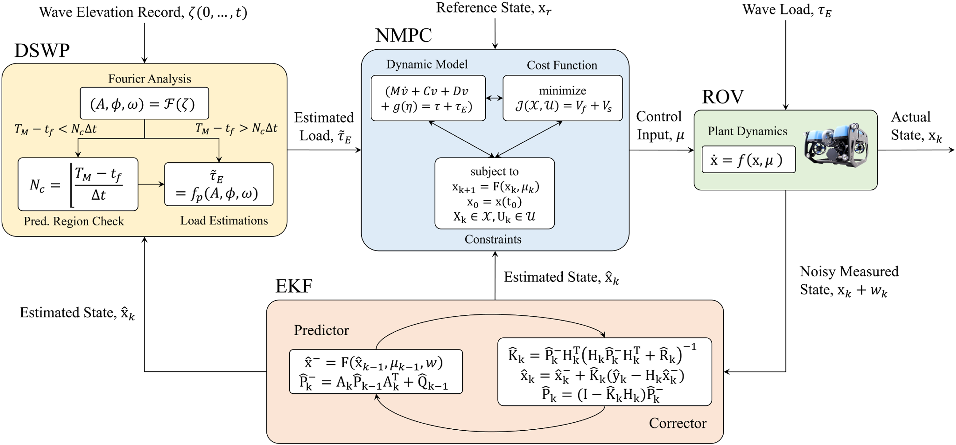
With reference to the above, this paper presents a complete end-to-end architecture for fast prediction and rejection of wave-induced hydrodynamic loading on an ROV by means of a nonlinear model predictive controller (NMPC). Here, we consider a preview of future time-varying disturbances, explicitly including these in the control action optimisation with the goal of improving station keeping control. This disturbance preview information can be transmitted from the measurement point to the vehicle (prediction point) using one of two methods (1) wireless transmission to a base station and relayed to the vehicle via a tether or (2) wireless transmission underwater directly to the vehicle, if operating untethered; see Figure 1. Both of these methods have benefits and drawbacks and are analysed further in Section 5.6. Conceptually, the framework entails the following strategy (see also Accompanying Video) schematically depicted in Figure 1: (a) measurements of sea surface elevation are accumulated at a fixed-location distant from the vehicle; (b) DSWP forms an estimate of the sea spectral parameters to predict the surface elevation at the vehicle location over a future time interval; (c) this information is transmitted to the vehicle using one of the two communication methods shown in Figure 1; (d) the future wave elevation profile at the vehicle is exploited to estimate the future time-varying hydrodynamic disturbances (leveraging previous validations detailed in (Walker et al., 2021a, 2021b)) at the vehicle’s depth which (e) are explicitly accounted for within the NMPC to yield a future sequence of optimised control actions. Information of the vehicle location is obtained through an extended Kalman filter (EKF) and the full strategy is tested across three different sea climates. Similarly, the performance of the control is analysed in the presence of varying levels of noise associated with the wave observer, along with varying degrees of time delay exhibited during communication between the measuring device and the vehicle, producing evidence of high robustness in the proposed method.

Figure 1.

Schematic representation of the proposed end-to-end protocol – the ROV receives predictive information relating to the oncoming wave from a measuring device upstream which the onboard control can exploit to compensate for future hydrodynamic disturbances. This information can be transmitted wireless to a base station and relayed to the ROV via a tether (communication option 1), or if operating untethered transmitted wireless directly underwater (communication option 2).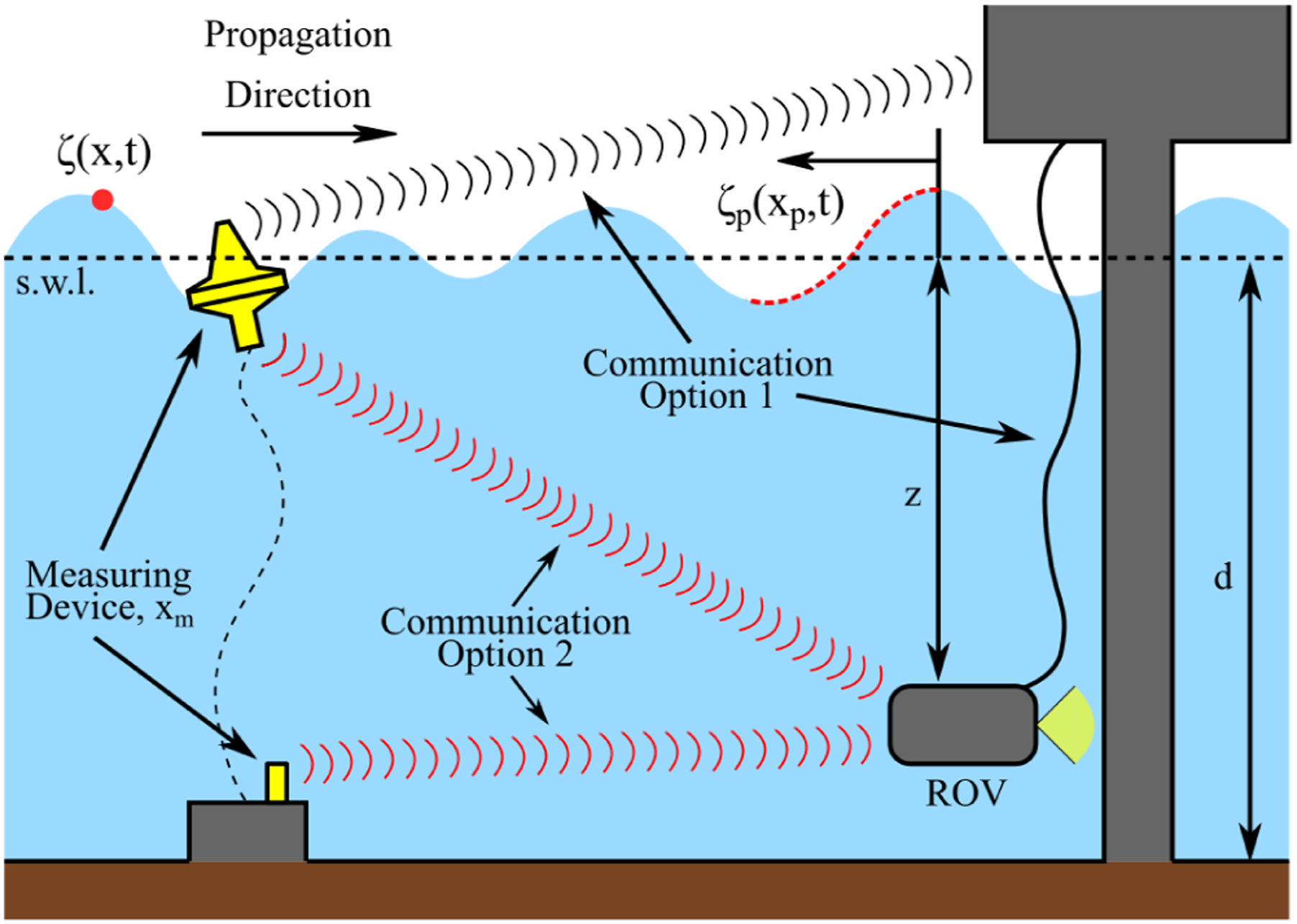

Ultimately, this work addresses the challenge of ROV operation in hazardous sea conditions by providing: (1) an experimental validation of a robust predictor for wave-induced disturbances over future, short-term, time-horizons; (2) the implementation of an NMPC architecture able to explicitly exploit the disturbance preview information to perform effective disturbance rejection; and (3) an in-depth analysis of the robustness of the proposed NMPC with preview method in handling noise and uncertainty, both in the elevation measurements and disturbance predictions. Conjunctionally, a discussion on the trade off in terms of power requirements during station keeping tasks is provided. This study proves the high potential associated with explicitly forming accurate future temporal wave predictions and implementing this directly within a real-time control scenario, providing a solution for close-quarters inspection and maintenance of shallow water offshore assets.

2. System modelling

2.1. Kinematics

The 6 degree-of-freedom (DoF) kinematics of the vehicle in the body-fixed frame relative to the earth-fixed frame is given by (Fossen, 1994):

$\dot{\mathit{\eta }}=\mathbf{J}(\mathit{\eta })\mathit{\nu }$

(1)

where $\mathit{\eta }\in {\mathbb{R}}^6$ is a state vector in the earth-fixed frame describing the position and orientation of the vehicle, $\mathit{\nu }\in {\mathbb{R}}^6$ is a state vector of linear and angular velocities in the body-fixed frame and $\mathbf{J}\in {\mathbb{R}}^{6\times 6}$ is a transformation matrix relating the two frames. The state vectors, shown in Figure 2, are explicitly defined as:

$\mathit{\eta }={\left[\begin{array}{cccccc}\hfill x\hfill & \hfill y\hfill & \hfill z\hfill & \hfill \varphi \hfill & \hfill \theta \hfill & \hfill \psi \hfill \end{array}\right]}^T$

(2)

$\mathit{\nu }={\left[\begin{array}{cccccc}\hfill u\hfill & \hfill v\hfill & \hfill w\hfill & \hfill p\hfill & \hfill q\hfill & \hfill r\hfill \end{array}\right]}^T$

(3)

where x, y and z describe the position of the vehicle in Cartesian co-ordinates; ϕ, θ and ψ describe the orientation of the vehicle in Euler angles; u, v and w represent linear velocities and p, q and r represent angular velocities. Given the equilibrium position of the vehicle at θ = 0 ^o , the constraints of J( η ) being undefined for θ = ±90 ^o represents a highly unlikely operating point and thus are assumed satisfied.

Figure 2.

The BlueROV2 heavy, labelled with SNAME notation and displaying the earth-fixed and body-fixed co-ordinate frames.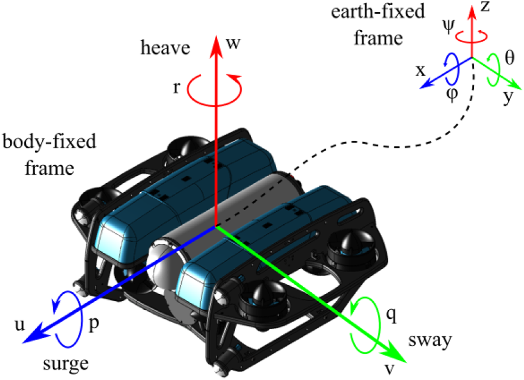

2.2. Dynamics

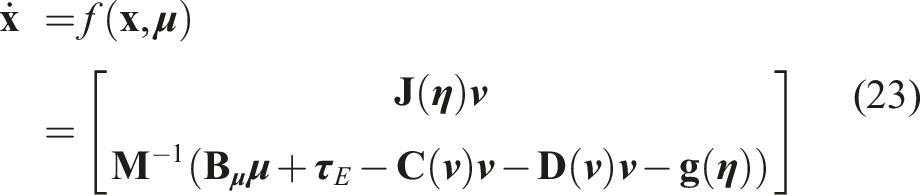
Considering the kinematic description in Section 2.1 and under the rigid-body approximation, the nonlinear dynamic behaviour for an underwater vehicle is described by:

$\mathbf{M}\dot{\mathit{\nu }}+\mathbf{C}(\mathit{\nu })\mathit{\nu }+\mathbf{D}(\mathit{\nu })\mathit{\nu }+\mathbf{g}(\mathit{\eta })=\mathit{\tau }+{\mathit{\tau }}_{\mathit{E}}$

(4)

where $\mathbf{M}\in {\mathbb{R}}^{6\times 6}$ is an inertia matrix, $\mathbf{C}(\mathit{\nu })\in {\mathbb{R}}^{6\times 6}$ is a matrix of Coriolis and centripetal terms, $\mathbf{D}(\mathit{\nu })\in {\mathbb{R}}^{6\times 6}$ is a hydrodynamic damping matrix, $\mathbf{g}(\mathit{\eta })\in {\mathbb{R}}^6$ is a vector of hydrostatic restoring forces, $\mathit{\tau }\in {\mathbb{R}}^6$ is a vector of external forces and moments (e.g. thrust) and ${\mathit{\tau }}_{\mathit{E}}\in {\mathbb{R}}^6$ is a vector of environmental disturbances, which in this instance arise from the presence of surface waves.

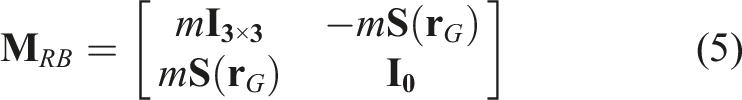
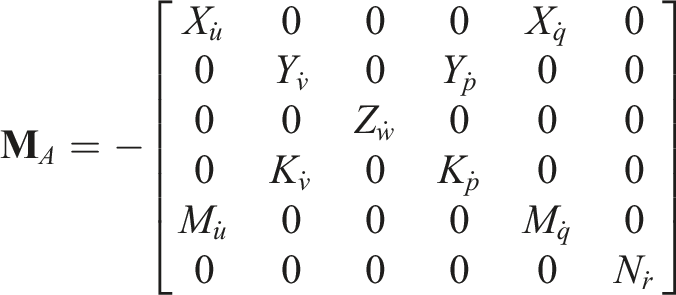
The inertia matrix is inclusive of added mass effects and is therefore defined as M = M _RB + M _A where M _RB is the rigid-body inertia matrix and M _A is the added-inertia matrix. In generalised compact form, the rigid-body inertia matrix is defined as:

${\mathbf{M}}_{RB}=\left[\begin{array}{cc}\hfill m{\mathbf{I}}_{\mathbf{3\times 3}}\hfill & \hfill -m\mathbf{S}({\mathbf{r}}_G)\hfill \\ \hfill m\mathbf{S}({\mathbf{r}}_G)\hfill & \hfill {\mathbf{I}}_{\mathbf{0}}\hfill \end{array}\right]$

(5)

where m is the vehicle dry mass, I_3×3 is an identity matrix, ${\mathbf{r}}_G={[x_G,y_G,z_G]}^T\in {\mathbb{R}}^3$ is the location of the vehicle’s centre of gravity and I₀ is the inertia tensor. S(−) is a skew-symmetric matrix.

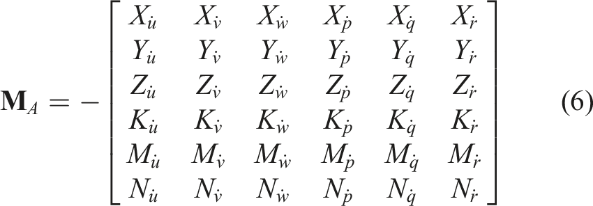
With respect to the added-inertia matrix, adopting the notation of SNAME (Fossen, 1994) it follows that:

${\mathbf{M}}_A=-\left[\begin{array}{cccccc}\hfill X_{\dot{u}}\hfill & \hfill X_{\dot{v}}\hfill & \hfill X_{\dot{w}}\hfill & \hfill X_{\dot{p}}\hfill & \hfill X_{\dot{q}}\hfill & \hfill X_{\dot{r}}\hfill \\ \hfill Y_{\dot{u}}\hfill & \hfill Y_{\dot{v}}\hfill & \hfill Y_{\dot{w}}\hfill & \hfill Y_{\dot{p}}\hfill & \hfill Y_{\dot{q}}\hfill & \hfill Y_{\dot{r}}\hfill \\ \hfill Z_{\dot{u}}\hfill & \hfill Z_{\dot{v}}\hfill & \hfill Z_{\dot{w}}\hfill & \hfill Z_{\dot{p}}\hfill & \hfill Z_{\dot{q}}\hfill & \hfill Z_{\dot{r}}\hfill \\ \hfill K_{\dot{u}}\hfill & \hfill K_{\dot{v}}\hfill & \hfill K_{\dot{w}}\hfill & \hfill K_{\dot{p}}\hfill & \hfill K_{\dot{q}}\hfill & \hfill K_{\dot{r}}\hfill \\ \hfill M_{\dot{u}}\hfill & \hfill M_{\dot{v}}\hfill & \hfill M_{\dot{w}}\hfill & \hfill M_{\dot{p}}\hfill & \hfill M_{\dot{q}}\hfill & \hfill M_{\dot{r}}\hfill \\ \hfill N_{\dot{u}}\hfill & \hfill N_{\dot{v}}\hfill & \hfill N_{\dot{w}}\hfill & \hfill N_{\dot{p}}\hfill & \hfill N_{\dot{q}}\hfill & \hfill N_{\dot{r}}\hfill \end{array}\right]$

(6)

where the individual coefficients describe added inertia effects related to the vehicle’s hydrodynamic properties. Similarly, the Coriolis and Centripetal matrix is defined as C( ν ) = C _RB ( ν ) + C _A ( ν ) where C _RB ( ν ) is the rigid-body contribution and C _A ( ν ) accounts for added inertia effects.

With respect to hydrodynamic damping, these effects can be conveniently grouped into contributions from linear and quadratic terms, ${\mathbf{D}}_L\left(\mathit{\nu }\right)\in {\mathrm{ℝ}}^{6\times 6}$ and ${\mathbf{D}}_Q\left(\mathit{\nu }\right)\in {\mathrm{ℝ}}^{6\times 6}$ , respectively. Thus:

$\mathbf{D}(\mathit{\nu })\mathit{\nu }=\{{\mathbf{D}}_L(\mathit{\nu })+{\mathbf{D}}_Q(\mathit{\nu })\odot |\mathit{\nu }|\}\mathit{\nu }$

(7)

Here, ⊙ represents the Hadamard product where each row of the matrix D _Q ( ν ) undergoes element-wise multiplication with the vector ν .

Finally, all terms arising from gravitational and buoyancy forces are grouped into a column vector dependent on the position of the vehicle centre of gravity (CoG), r _G , the vehicle centre of buoyancy (CoB), ${\mathbf{r}}_B={[x_B,y_B,z_B]}^T$ and the orientation of the vehicle. The resulting vector is given as:

$\mathbf{g}(\mathit{\eta })=\left[\begin{array}{c}\hfill (W-B)s\theta \hfill \\ \hfill -(W-B)c\theta s\varphi \hfill \\ \hfill -(W-B)c\theta c\varphi \hfill \\ \hfill -(y_{G}W-y_{B}B)c\theta c\varphi +(z_{G}W-z_{B}B)c\theta s\varphi \hfill \\ \hfill -(z_{G}W-z_{B}B)s\theta +(x_{G}W-x_{B}B)c\theta c\varphi \hfill \\ \hfill -(x_{G}W-x_{B}B)c\theta s\varphi -(y_{G}W-y_{B}B)s\theta \hfill \end{array}\right]$

(8)

where W and B are the vehicle weight and buoyancy and notations $c\varphi ,s\varphi$ are abbreviations for $\cos \varphi ,\sin \varphi$ respectively. The vehicle dynamics can be simplified based on the following assumptions:

Assumption 2.1

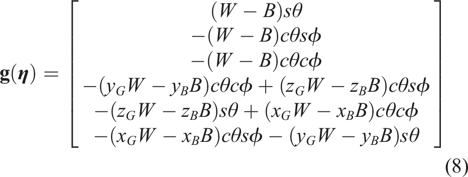
The centre of gravity (CoG) of the vehicle is aligned with the origin of the body-fixed frame:

${\mathbf{r}}_G={[x_G,y_G,z_G]}^T={[\mathrm{0,0,0}]}^T$

(9)

Assumption 2.2

The centre of buoyancy (CoB) of the vehicle is assumed to be aligned with the origin in the longitudinal and lateral axes:

${\mathbf{r}}_B={[x_B,y_B,z_B]}^T={[\mathrm{0,0},z_B]}^T$

(10)

Assumption 2.3

The vehicle is considered to possess two planes of symmetry, fore-aft and port-starboard, owing to the vehicle design, thus the added mass matrix can be reduced to:

${\mathbf{M}}_A=-\left[\begin{array}{cccccc}\hfill X_{\dot{u}}\hfill & \hfill 0\hfill & \hfill 0\hfill & \hfill 0\hfill & \hfill X_{\dot{q}}\hfill & \hfill 0\hfill \\ \hfill 0\hfill & \hfill Y_{\dot{v}}\hfill & \hfill 0\hfill & \hfill Y_{\dot{p}}\hfill & \hfill 0\hfill & \hfill 0\hfill \\ \hfill 0\hfill & \hfill 0\hfill & \hfill Z_{\dot{w}}\hfill & \hfill 0\hfill & \hfill 0\hfill & \hfill 0\hfill \\ \hfill 0\hfill & \hfill K_{\dot{v}}\hfill & \hfill 0\hfill & \hfill K_{\dot{p}}\hfill & \hfill 0\hfill & \hfill 0\hfill \\ \hfill M_{\dot{u}}\hfill & \hfill 0\hfill & \hfill 0\hfill & \hfill 0\hfill & \hfill M_{\dot{q}}\hfill & \hfill 0\hfill \\ \hfill 0\hfill & \hfill 0\hfill & \hfill 0\hfill & \hfill 0\hfill & \hfill 0\hfill & \hfill N_{\dot{r}}\hfill \end{array}\right]$

Assumption 2.4

The damping matrix can be simplified to purely diagonal-form due to the vehicle symmetry, where the remaining off-diagonal elements after Assumption 2.3 are assumed negligible:

$X_q,X_{q|q|},Y_p,Y_{p|p|},K_v,K_{v|v|},M_u,M_{u|u|}\approx 0$

${\mathbf{D}}_L(\mathit{\nu })=-\mathrm{d}\mathrm{i}\mathrm{a}\mathrm{g}\{X_u,Y_v,Z_w,K_p,M_q,N_r\}$

${\mathbf{D}}_Q(\mathit{\nu })-\mathrm{d}\mathrm{i}\mathrm{a}\mathrm{g}\{X_{u|u|},Y_{v|v|},Z_{w|w|},K_{p|p|},M_{q|q|},N_{r|r|}\}$

2.3. Wave-induced disturbances

The focused applications of our proposed method are based in shallow water environments where wave breaking is not occurring, but where wave disturbances are prominent across the upper section of the water column. To account for hydrodynamic forcing from random sea states, a second-order model of the wave elevation and particle trajectories beneath the sea surface is adopted. In the cases considered throughout this work, the wave elevation is modelled to propagate in a single direction and can be considered as a planar two dimensional wave.

Assumption 2.5

Ocean waves are considered to propagate uni-directionally and interact with the vehicle head-on, allowing simplification to a planar case in relation to the vehicle dynamics.

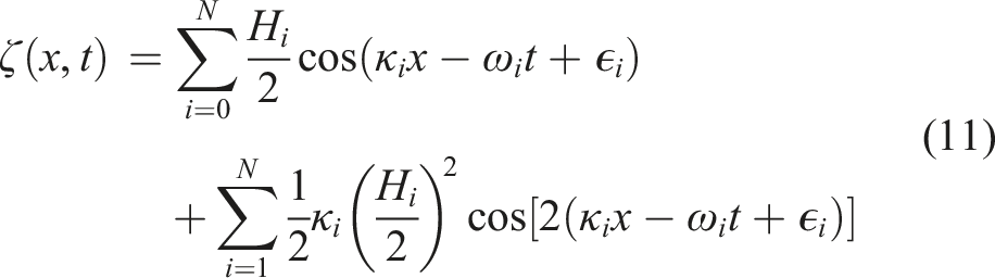
Assuming that the sea state can be described by a spectrum of N monochromatic components, each with a unique wave height, H, period, T, and phase offset, ϵ and that the second-order effects can be linearly superimposed (McCormick, 2010), the surface elevation at a point (x, t) in space and time is described by:

$\begin{array}{ll}\hfill \zeta (x,t)& =\sum _{i=0}^N\frac{H_i}{2}\cos ({\kappa }_{i}x-{\omega }_{i}t+{ϵ}_i)\hfill \\ \hfill & +\sum _{i=1}^N\frac{1}{2}{\kappa }_i{\left(\frac{H_i}{2}\right)}^2\cos [2({\kappa }_{i}x-{\omega }_{i}t+{ϵ}_i)]\hfill \end{array}$

(11)

where κ and ω represent the wave number and the angular frequency, respectively, solved for by consideration of the dispersion relation:

${\omega }_i=\sqrt{g{\kappa }_i\tanh {\kappa }_{i}d}$

(12)

where g and d are the gravitational constant and seabed depth.

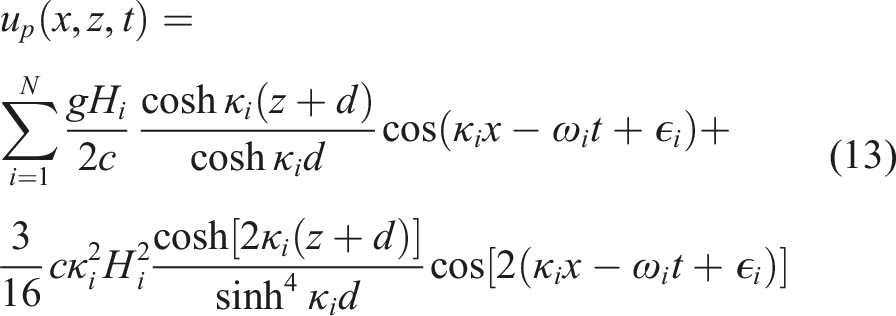
Spectral information also facilitates deduction of the particle velocities in the global frame, which for the surge and heave components are given by

$\begin{array}{ll}\hfill & u_p(x,z,t)=\hfill \\ \hfill & \sum _{i=1}^N\frac{g{H}_i}{2c}\frac{\cosh \hspace{0.17em}{\kappa }_i(z+d)}{\cosh \hspace{0.17em}{\kappa }_{i}d}\cos ({\kappa }_{i}x-{\omega }_{i}t+{ϵ}_i)+\hfill \\ \hfill & \frac{3}{16}c{\kappa }_i^2{H}_i^2\frac{\cosh [2{\kappa }_i(z+d)]}{{\sinh }^4{\kappa }_{i}d}\cos [2({\kappa }_{i}x-{\omega }_{i}t+{ϵ}_i)]\hfill \end{array}$

(13)

$\begin{array}{ll}\hfill & w_p(x,z,t)=\hfill \\ \hfill & \sum _{i=1}^N\frac{g{H}_i}{2c}\frac{\sinh \hspace{0.17em}{\kappa }_i(z+d)}{\cosh \hspace{0.17em}{\kappa }_{i}d}\sin ({\kappa }_{i}x-{\omega }_{i}t+{ϵ}_i)+\hfill \\ \hfill & \frac{3}{16}c{\kappa }_i^2{H}_i^2\frac{\sinh [2{\kappa }_i(z+d)]}{{\sinh }^4{\kappa }_{i}d}\sin [2({\kappa }_{i}x-{\omega }_{i}t+{ϵ}_i)]\hfill \end{array}$

(14)

where z ∈ [−d, 0] and c are the evaluated depth and celerity, respectively. The definition for celerity is dependent on the seabed depth, d, to wavelength, λ, ratio as follows (Reeve et al., 2004):

$c(\omega )=\left\{\begin{array}{cc}\sqrt{(g\lambda )/2\pi },\hfill & \text{if}d/\lambda \ge 0.5\hfill \\ \sqrt{gd},\hfill & \text{if}d/\lambda \le 0.05\hfill \\ \sqrt{(g/\kappa )\tanh \kappa d},\hfill & \text{if}0.5>d/\lambda >0.05\hfill \end{array}\right.$

The solutions of equations (13) and (14) and their derivatives are the primary inputs to the system dynamics for modelling the vehicle behaviour by defining ${\mathit{\nu }}_p={\left[{\nu }_{p,x},{\nu }_{p,z}\right]}^T={\mathbf{R}}_y^T(\theta ){\left[u_p,w_p\right]}^T$ (where R _y (θ) is a rotation matrix) yielding

${\mathit{\tau }}_E=\left[\begin{array}{c}\hfill X_E\hfill \\ \hfill Z_E\hfill \\ \hfill M_E\hfill \end{array}\right]=\left[\begin{array}{c}\hfill X_{\dot{u}}{\dot{\nu }}_{p,x}+\{X_u+X_{u|u|}|{\nu }_{p,x}|\}{\nu }_{p,x}\hfill \\ \hfill Z_{\dot{w}}{\dot{\nu }}_{p,z}+\{Z_w+Z_{w|w|}|{\nu }_{p,z}|\}{\nu }_{p,z}\hfill \\ \hfill {\int }_{-L/2}^{L/2}{Z}_E(x^{\prime },z^{\prime },t)x^{\prime }dx\hfill \end{array}\right]$

(15)

where L is the vehicle body length and (x′, z′) refers to the position of evaluation in the vehicle’s local frame, allowing for an unsteady flow to be accounted for across the body length with respect to the pitch disturbance. This approach was experimentally validated in previous work (Gabl et al., 2020, 2021; Walker et al., 2021a, 2021b) and was shown to produce accurate and computationally inexpensive estimations of the wave-induced forces and moments on an ROV. This approach lends itself to near real-time short-horizon predictions of impending wave disturbances, enabling effective implementation in predictive control schemes.

As this work is an initial investigation of the proposed methodology and for the sake of demonstration, the analysis herein is restricted to a planar case focusing on uni-directional waves where disturbances to the sway, roll and yaw motion are negligible. Therefore, these can be regulated without explicit consideration in the optimised control. Therefore, the predictive strategy detailed henceforth is only applied to the surge, heave and pitch. Extension to a multi-directional wave case can be achieved by considering a sparse array of wave buoys rather than just a single point of measurement, for example, using the PTPD (Fernandes et al., 2000) or SPAIR method (Draycott et al., 2016).

3. Wave disturbance prediction

Short temporal prediction of future disturbances facilitates the inclusion of preview information within the control problem, framing this as an optimisation over a time horizon for which an optimal control trajectory can be calculated. To enable this kind of anticipatory control, a dedicated predictor of oncoming disturbances is required. As alluded to earlier, forming predictions ahead of time before the vehicle is subjected to any wave disturbances is crucial for inclusion in an NMPC scheme. The disturbance predictor proposed here relies on deterministic sea wave prediction (DSWP) (Al-Ani et al., 2020; Belmont et al., 2006a, 2006b) and specifically the fixed-point method. This method entails on-line inference of the sea state spectral parameters to produce short term forecasts of the future sea surface elevation at a point of interest, based purely on prior measurements of the wave temporal profile at some distance from the vehicle’s location.

3.1. Fixed-point deterministic sea wave prediction

The fixed-point variant of DSWP employed in this work accumulates temporal data over a period T _M from a fixed location upstream of the vehicle at a distance x _P , subsequently producing a prediction of the wave elevation and particle trajectories at the vehicle location, Figure 1. The sea surface is assumed statistically stationary for a time duration longer than the actual prediction window. Therefore, spectral parameters can be exploited to determine the sea state properties. 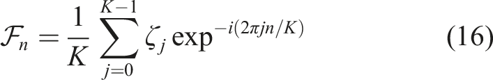By defining the wave measuring point as x _M = 0, the sea-state frequency spectrum can be obtained by considering a wave-height record ${\zeta }_M=\zeta (0,\left[t_0,t_0+\mathrm{\Delta }t,\dots ,T_M\right])$ discretized by steps of Δt:

${\mathcal{F}}_n=\frac{1}{K}\sum _{j=0}^{K-1}{\zeta }_j{\exp }^{-i(2\pi jn/K)}$

(16)

where K = T _M $/$ Δt is the number of wave-height samples in the wave-height record. Given these Fourier coefficients, the prediction model is obtained by consideration of equation (11) with the vehicle location x _V as an input, producing the predicted temporal evolution of the sea surface elevation at the vehicle location:

$\begin{array}{ll}\hfill \tilde{\zeta }(x_V,t)& =\sum _{n=0}^N{A}_n\cos ({\kappa }_n{x}_V-{\omega }_{n}t+{ϵ}_n)\hfill \\ \hfill & +\sum _{n=0}^N\frac{1}{2}{\kappa }_n{A}_n^2\cos 2({\kappa }_n{x}_V-{\omega }_{n}t+{ϵ}_n)\hfill \end{array}$

(17)

with

$A_n=|{\mathcal{F}}_n|{ϵ}_n=\angle {\mathcal{F}}_n{\kappa }_n={\omega }_n^2/g$

${\omega }_n\in \left[\frac{2\pi n}{K\mathrm{\Delta }t},\frac{2\pi (n+1)}{K\mathrm{\Delta }t},\dots ,\frac{2\pi }{K\mathrm{\Delta }t}(K-1)\right]$

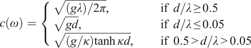
For shallow water waves, the limit of the dispersion relation takes the form lim_d→∞ κ² → ω² $/$ gd, resulting in a linear phase filter where κ _n x _V is considered a phase-shifting parameter for propagating the wave through space (Belmont et al., 2006a). Given the amplitude spectrum, the transformation into the power density representation is straight forward:

$S_n=\frac{A_n^2}{2\mathrm{\Delta }\omega }$

(18)

where Δω = 2π/KΔt.

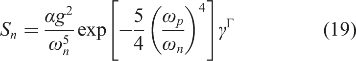
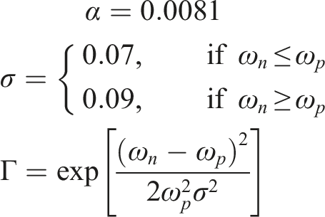
Several well-known spectral representation are typically used, the two most common being the JONSWAP and the Pierson-Moskowitz. In this work, the JONSWAP definition is adopted to model the sea state and therefore this is assumed to be the ideal form returned by equation (18). The JONSWAP representation is defined by:

$S_n=\frac{\alpha g^2}{{\omega }_n^5}\exp \left[-\frac{5}{4}{\left(\frac{{\omega }_p}{{\omega }_n}\right)}^4\right]{\gamma }^{\mathrm{\Gamma }}$

(19)

where ω _p is the spectral peak frequency, γ is the Phillips constant and

$\alpha =0.0081\sigma =\left\{\begin{array}{cc}0.07,\hfill & \text{if}{\omega }_n\le {\omega }_p\hfill \\ 0.09,\hfill & \text{if}{\omega }_n\ge {\omega }_p\hfill \end{array}\right.\mathrm{\Gamma }=\exp \left[\frac{{({\omega }_n-{\omega }_p)}^2}{2{\omega }_p^2{\sigma }^2}\right]$

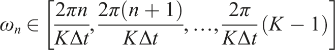
A key consideration when forming the prediction requirements and capabilities of the algorithm is to deduce the maximum length that the prediction will be valid, in accordance with the assumption of statistical stationarity of the sea state. This is dictated by the space-time diagram for the system, with an example shown in Figure 3. By analysing the celerity of the spectral components with the minimum and maximum frequency, the predictable region can be determined. To extend the prediction length, the wave spectrum is bounded such that components with minimal influence on the resulting waveform are disregarded.

Figure 3.

Space-time diagram for the fixed point method, where the grey area represents the region in which a prediction can be obtained. Here, x_p,max is the distance at which a prediction of maximum time, t_p,max is obtainable and d_max is the furthest point from the measurement site where the prediction can be considered reliable.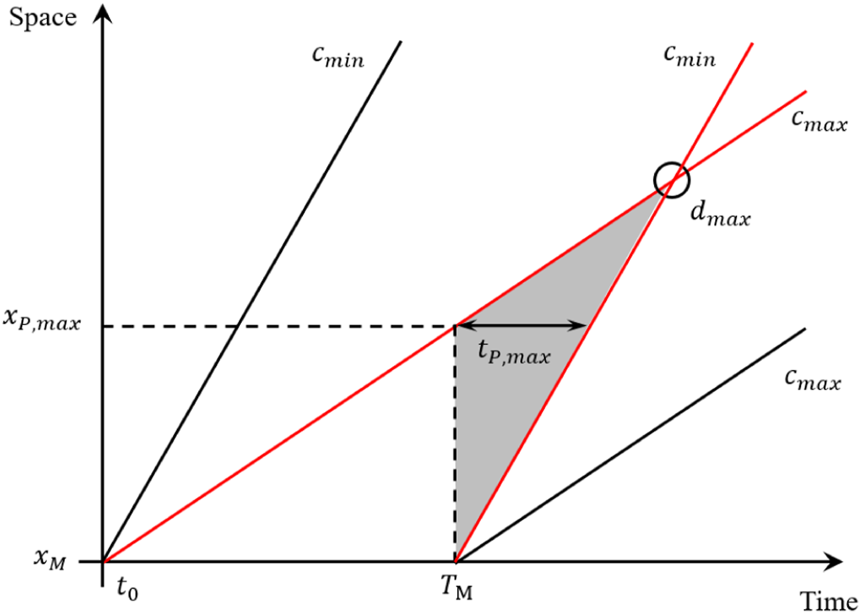

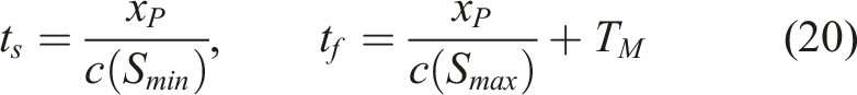
For any sea state, a wave spectrum S _n can be identified such that bounding frequency components f _min and f _max can be prescribed, respectively, correspondent to spectral components S _min and S _max . Following this, the maximum valid predictable region can be determined with reference to the time-frame t _s → t _f :

$t_s=\frac{x_P}{c(S_{\mathit{min}})},t_f=\frac{x_P}{c(S_{\mathit{max}})}+T_M$

(20)

Any prediction outwith this time-frame cannot be considered reliable and therefore the prediction is deemed to be invalid. Most importantly, T _M and t _f dictate a cut-off temporal threshold for the time scale of the receding horizon in the NMPC.

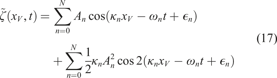
From the estimated spectral representation of the sea-state, equation (17) can be considered to predict the particle trajectories at the vehicle location beneath the surface, substituting x _V into equations (13) and (14) to obtain ${\tilde{\mathit{\nu }}}_p=\left[\begin{array}{c}\hfill {\tilde{\nu }}_{p,x},{\tilde{\nu }}_{p,z}\hfill \end{array}\right]$ . The prediction of environmental disturbances can then be obtained by considering:

${\tilde{\mathit{\tau }}}_E=\left[\begin{array}{c}\hfill {\tilde{X}}_E\hfill \\ \hfill {\tilde{Z}}_E\hfill \\ \hfill {\tilde{M}}_E\hfill \end{array}\right]=\left[\begin{array}{c}\hfill X_{\dot{u}}{\dot{\tilde{\nu }}}_{p,x}+\left(X_u+X_{u|u|}|{\tilde{\nu }}_{p,x}|\right){\tilde{\nu }}_{p,x}\hfill \\ \hfill Z_{\dot{w}}{\dot{\tilde{\nu }}}_{p,z}+\left(Z_w+Z_{w|w|}|{\tilde{\nu }}_{p,z}|\right){\tilde{\nu }}_{p,z}\hfill \\ \hfill {\int }_{-L/2}^{L/2}{\tilde{Z}}_E(x^{\prime },z^{\prime },t)x^{\prime }dx\hfill \end{array}\right]$

(21)

This forms the complete process from the initial recorded wave height measurements through to the propagation and evaluation of hydrodynamic loading at the vehicle location. This is given in compact form as Algorithm 1.

3.2. Experimental validation

As our application is tailored towards short horizon dynamic control, it was desirable to understand the physical limitations of the predictable region and the accuracy of the estimated temporal wave evolution. To this end, an experimental study was conducted at the FloWave Ocean Energy Research Facility at the

Algorithm 1. Fixed-Point Deterministic Sea Wave Prediction with Wave-induced Disturbance Estimation Algorithm

University of Edinburgh (Ingram et al., 2014). The study consisted of three irregular wave trains (JONSWAP spectra) generated by the wave-makers and propagated across the diameter of the tank, with the parameters of these given in Table 1. The purpose of the experiment was to predict the time evolution of wave elevation at a fixed location by relying on a continuous measurement at a fixed point upstream.

Table 1.

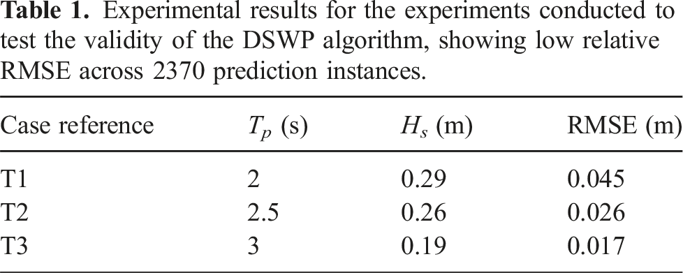
Experimental results for the experiments conducted to test the validity of the DSWP algorithm, showing low relative RMSE across 2370 prediction instances.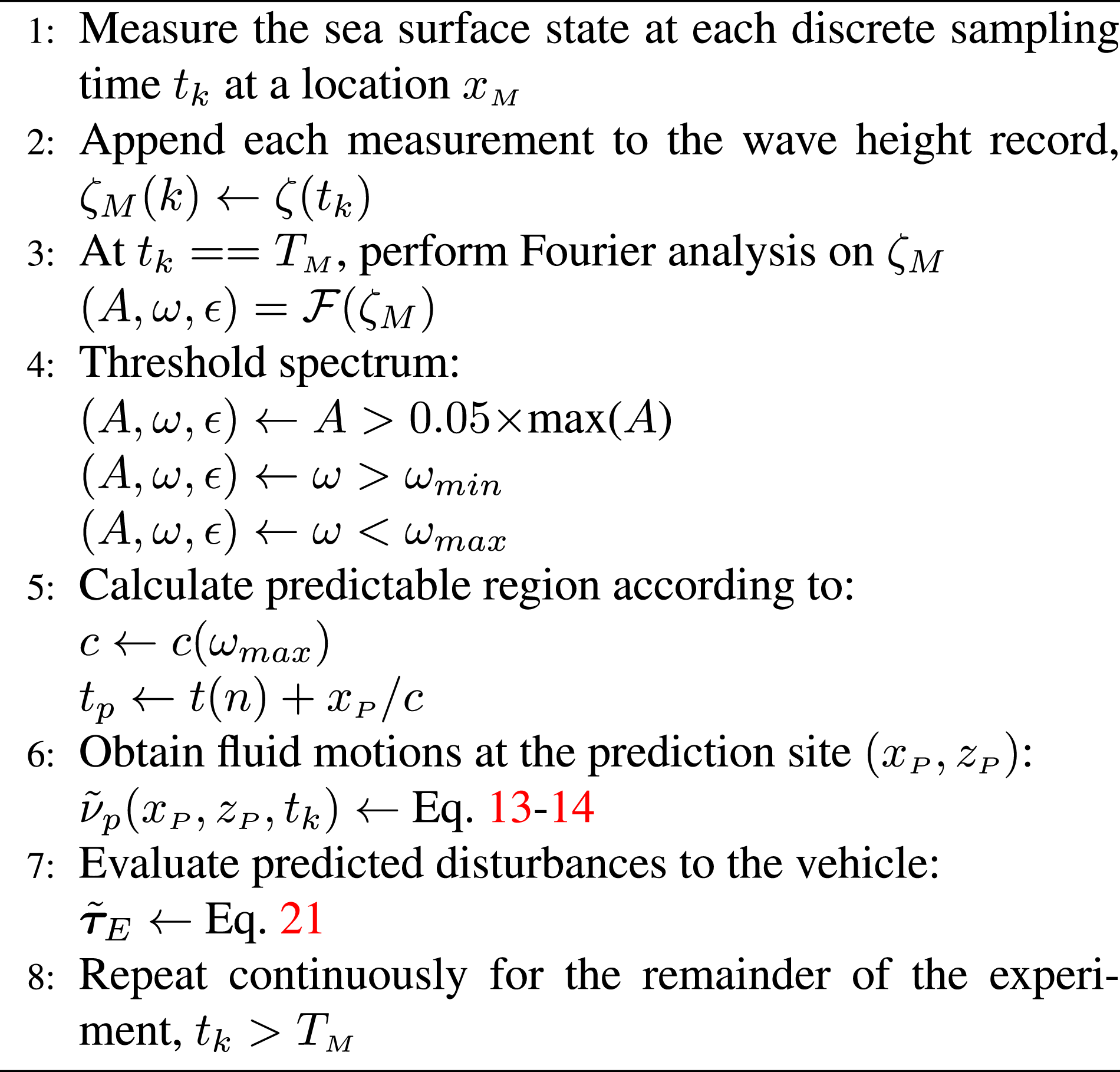

Case reference	T p (s)	H s (m)	RMSE (m)
T1	2	0.29	0.045
T2	2.5	0.26	0.026
T3	3	0.19	0.017

Due to the physical limits of the tank, the length of waves attainable was limited at the expense of larger wave height. A five-piece conductive wave gauge array was placed coincident to the propagation direction, with each unit equally spaced by 3.77m and with a maximum of 15.08m between the two furthest wave gauges (WG), indicated as WG1 and WG5. A gauge at the centre of the tank, WG3, was used as a reference position of 0m to align with the reference of the tank software when generating the wave formation. See Figure 4 for a visual representation of the arrangement stating the gauge labels and showing a recorded snapshot of a wave from case W2. The wave gauges monitoring the surface elevation have an accuracy smaller than 1 mm (MARINET, 2012), with a standard calibration of five points covering ± 100 mm conducted to ensure this high accuracy. Data collection and transfer is computationally inexpensive (Gabl et al., 2019), confirming its suitability for real-time usage as part of the disturbance preview formulation and control optimisation loop. The wave was recorded at each gauge location throughout the experiment duration of $\approx 500$ s, providing a basis to test the DSWP algorithm by attempting to predict the wave formation at WG5 using only temporal measurements at WG1.

Figure 4.

Experimental example of obtaining the results shown in Figure 5 and Table 1, displaying (a) a snapshot of the recorded wave train from the side-view, (b) wave gauge locations and wave height with respect to the tank x-axis from the top view, and (c) the experimental set-up. Due to Assumption 2.5 the wave is uniform across the tank y-axis, as shown in subplot (b).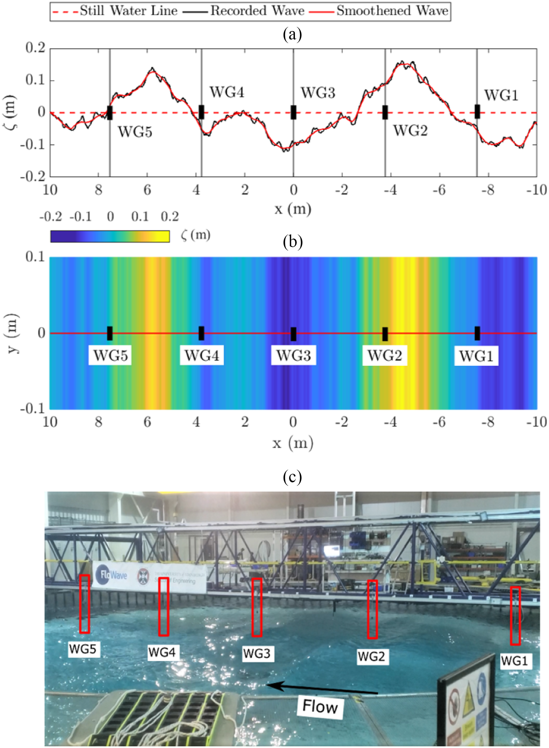

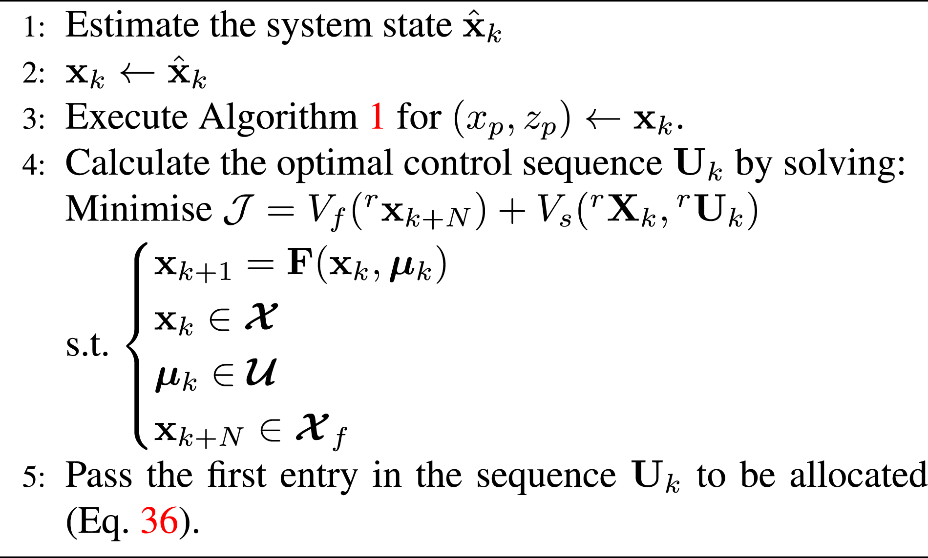
To analyse the accuracy of the DSWP algorithm, the root-mean-square-error (RMSE) of the wave elevation within the predicted region was evaluated by taking a prediction at each time-step and summarising the mean RMSE across all predictions. During this analysis, the first 300s of wave-height measurements at WG1 was accumulated before attempting to form predictions during the final 200s of the trial as a rolling temporal window relative to the length of the predictable region attainable. In Algorithm 1, the initial steps 1 and 2 refer to the initial accumulation stage. To maintain consistency, a sliding window was applied meaning only the previous 300s of wave measurements prior to the current time-step were used in the prediction process. The data was discretized at a rate of 16Hz, thus the analysis concerns 3,600 individual predictions – the reconstructed spectrum was bounded between f_min = 0.2Hz and f_max = 2Hz, allowing a predictable region of $\approx 2$ s to be obtained (which would be sufficient for the NMPC to be effective).

The RMSE reported in Table 1 clearly indicates that DSWP is capable of estimating the wave height at the prediction site with high accuracy. The maximum RMSE of 0.045m refers to the wave with the shortest period, confirming that longer waves which are better approximated by a linear swell model are predicted with higher accuracy. This is convenient for control applications, as wavelength tends to increase with significant wave height and energetic climate conditions typically relate to spectra with larger peak periods. A set of rolling temporal prediction snapshots relating to case T2 are depicted in Figure 5, showing the measured wave elevation at WG5 against the prediction based on only measurements at WG1. Within Figure 5, a prediction is shown prior to the current time-step which can be explained by referring to equation (20). The time-frame t _s → t _f dictates the length where the assumption of statistical stationarity holds at the prediction site, thus also includes reconstruction of past wave elevations. The additional predicted section of the wave elevation arises from the shift in space (defined by the filter parameter κ _n x). Each snapshot indicates the current time and the horizon over which prediction is performed, offering confidence in the capability of the predictor to generate a reliable temporal evolution of the sea surface at the point of interest.

Figure 5.

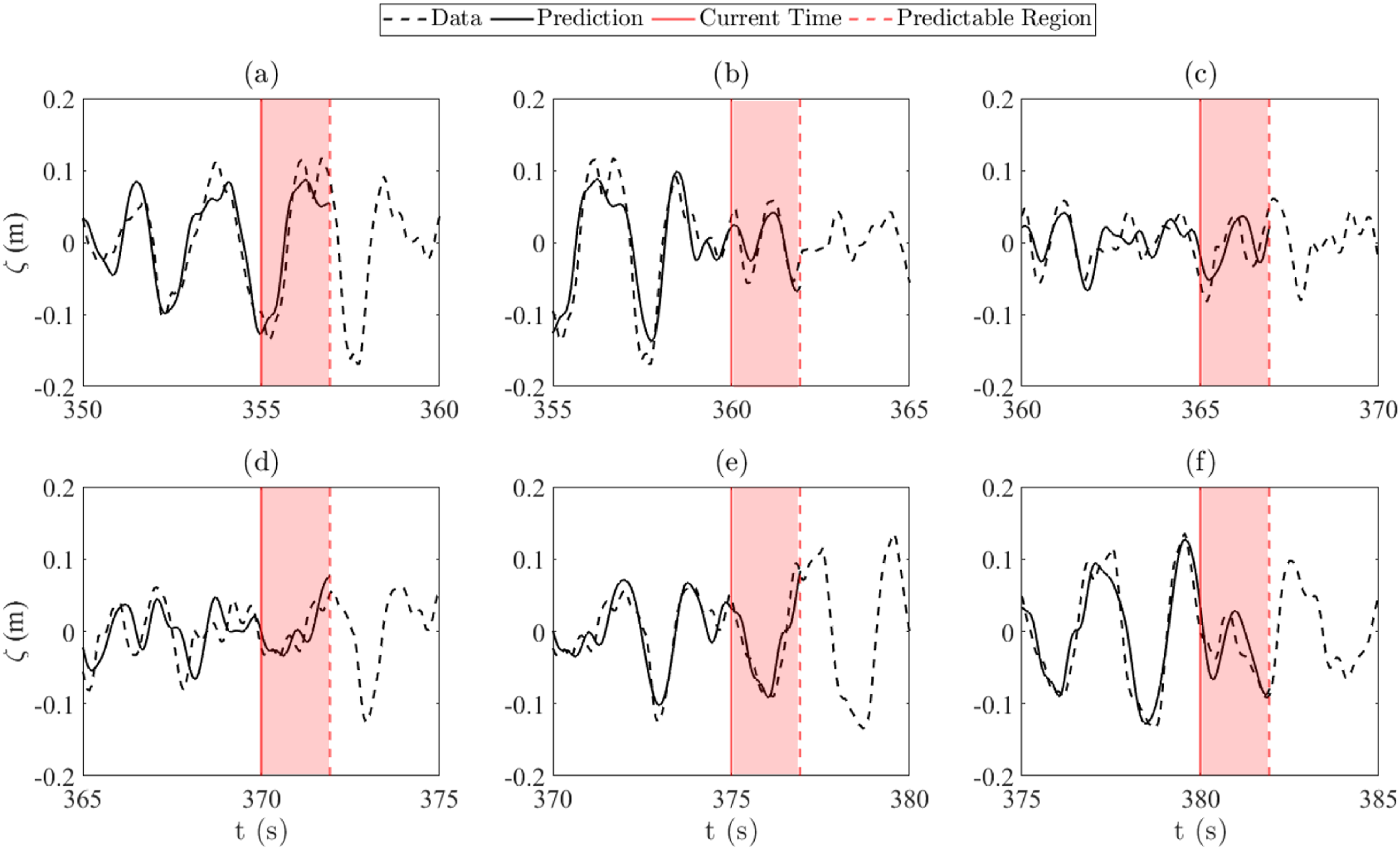
Various instances showing the DSWP algorithm producing accurate short-term predictions ( $\approx 2$ s) of the temporal wave-height, where the prediction is formed exclusively based on measurements from a wave gauge ≈ 15 m upstream. Subplots (a–f) show different predicted snapshots as the wave evolves in time. The red shaded area is the interval over which wave prediction in the future is regarded as reliable, t_p,max based on the given wave parameters (see also Accompanying Video).

4. Nonlinear model predictive control

Given the results obtained from the prediction algorithm, the controller adopted for performing the station keeping task was a nonlinear model predictive controller (NMPC) coupled with an EKF for performing state estimation. This section details formulation of the optimal control problem.

4.1. NMPC formulation

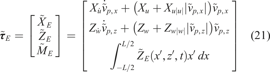
With reference to the theoretical model described in Section 2, the system state is defined as the position and velocity of the vehicle such that

$\mathbf{x}=\left[\begin{array}{c}\hfill \mathit{\eta }\hfill \\ \hfill \mathit{\nu }\hfill \end{array}\right]$

(22)

The nonlinear dynamics are therefore described by the function:

$\begin{array}{ll}\hfill \dot{\mathbf{x}}& =f(\mathbf{x},\mathit{\mu })\hfill \\ \hfill & =\left[\begin{array}{c}\hfill \mathbf{J}(\mathit{\eta })\mathit{\nu }\hfill \\ \hfill {\mathbf{M}}^{-1}({\mathbf{B}}_{\mathit{\mu }}\mathit{\mu }+{\mathit{\tau }}_E-\mathbf{C}(\mathit{\nu })\mathit{\nu }-\mathbf{D}(\mathit{\nu })\mathit{\nu }-\mathbf{g}(\mathit{\eta }))\hfill \end{array}\right]\hfill \end{array}$

(23)

where x and μ represent the system state and control input. Equation (23) is then time-discretized and solved via fourth-order Runge-Kutta integration:

${\mathbf{x}}_{k+1}=F({\mathbf{x}}_k,{\mathit{\mu }}_{\mathit{k}})$

(24)

where each step k represents a timestep Δt and F(⋅) describes the discrete dynamics function, in contrast to the continuous representation f (⋅). The predicted trajectories for the prediction horizon of N _c steps are then represented as a sequence of states and control inputs such that:

${\mathbf{X}}_k=\left[\begin{array}{c}\hfill F({\mathbf{x}}_k,{\mathit{\mu }}_{\mathit{k}})\hfill \\ \hfill F({\mathbf{x}}_{k+1},{\mathit{\mu }}_{\mathit{k}+\mathbf{1}})\hfill \\ \hfill ⋮\hfill \\ \hfill F({\mathbf{x}}_{k+N_c-1},{\mathit{\mu }}_{\mathit{k}+{\mathit{N}}_{\mathit{c}}-\mathbf{1}})\hfill \end{array}\right]$

(25)

${\mathbf{U}}_k={\left[\begin{array}{cccc}\hfill {\mathit{\mu }}_k,\hfill & \hfill {\mathit{\mu }}_{k+1},\hfill & \hfill \dots ,\hfill & \hfill {\mathit{\mu }}_{k+N-1}\hfill \end{array}\right]}^T$

(26)

where ${\mathbf{x}}_k\in \mathcal{X}$ and ${\mathit{\mu }}_k\in \mathcal{U}$ represents feasible sets related to the defined system constraints. With reference to equation (20), inclusion of disturbance preview information is reliant on T _M − t _f > N _c Δt, that is, the prediction horizon of the NMPC cannot be longer than the wave prediction window. In the event that this inequality is not satisfied, N _c can be adjusted online according to Figure 6.

Figure 6.

The proposed framework for predictive disturbance mitigation, showing each element in block diagram format. In the DSWP block, f _p is a function which transforms the spectral parameters into wave loading – see equation (21).

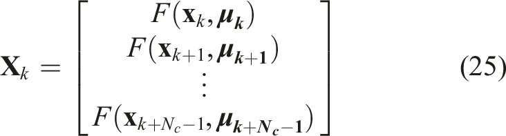
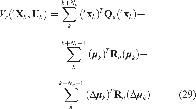
From this, the NMPC can be formulated for reference tracking using a quadratic cost function, by defining a reference state, 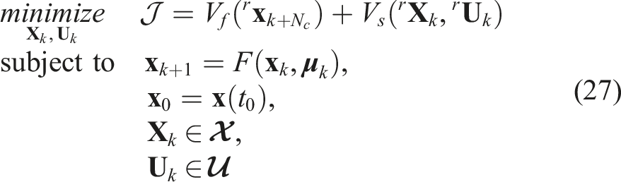x _r . The optimal control problem inclusive of a terminal cost can then be formulated as:

$\begin{array}{ll}\underset{{\mathbf{X}}_k,{\mathbf{U}}_k}{minimize}\hfill & \mathcal{J}=V_f({}^r\mathbf{x}_{k+N_c})+V_s({}^r\mathbf{X}_k,{}^r\mathbf{U}_k)\hfill \\ \mathrm{s}\mathrm{u}\mathrm{b}\mathrm{j}\mathrm{e}\mathrm{c}\mathrm{t}\mathrm{t}\mathrm{o}\hfill & {\mathbf{x}}_{k+1}=F({\mathbf{x}}_k,{\mathit{\mu }}_k),\hfill \\ {\mathbf{x}}_0=\mathbf{x}(t_0),\hfill \\ {\mathbf{X}}_k\in \mathcal{X},\hfill \\ {\mathbf{U}}_k\in \mathcal{U}\hfill \end{array}$

(27)

Here, ^r x _k = x _r − x _k and x (t₀) is the initial system state. Also, V _f and V _s are functions representing the terminal and stage costs, respectively, such that:

$V_f({}^r\mathbf{x}_{k+N_c})={({}^r\mathbf{x}_{k+N_c})}^T{\mathbf{P}}_{\mathbf{x}}({}^r\mathbf{x}_{k+N_c})$

(28)

$\begin{array}{ll}\hfill V_s({}^r\mathbf{X}_k,{\mathbf{U}}_k)& =\sum _k^{k+N_c}{({}^r\mathbf{x}_k)}^T{\mathbf{Q}}_{\mathbf{x}}({}^r\mathbf{x}_k)+\hfill \\ \hfill & \sum _k^{k+N_c-1}{({\mathit{\mu }}_k)}^T{\mathbf{R}}_{\mu }({\mathit{\mu }}_k)+\hfill \\ \hfill & \sum _k^{k+N_c-1}{(\mathrm{\Delta }{\mathit{\mu }}_k)}^T{\mathbf{R}}_{\mu }(\mathrm{\Delta }{\mathit{\mu }}_k)\hfill \end{array}$

(29)

where ${\mathbf{P}}_{\mu }\in {\mathbb{R}}^{3\times 3}$ , ${\mathbf{Q}}_{\mathbf{x}}\in {\mathbb{R}}^{3\times 3}$ and ${\mathbf{R}}_{\mu }\in {\mathbb{R}}^{3\times 3}$ are weighting matrices on the terminal state, intermediate state and control. Inclusion of this terminal cost on the final state in the optimisation sequence helps facilitate recursive feasibility and improved stability within the control problem (Mayne et al., 2000). Implementation of the NMPC scheme was performed using the CasADi Matlab library in conjunction with the IPOPT solver (Andersson et al., 2019), using a direct multiple shooting method, given in Algorithm 2.

4.2. Integrated architecture

The NMPC and DSWP formulation assumes that the vehicle state is known in order to compute the wave-induced disturbances and subsequently the optimal trajectory. Hence, knowledge of the vehicle instantaneous position is key to the performance of the proposed system: a poor state estimation will yield a poor wave prediction. In real-world operations the vehicle’s absolute state is obtained from sensor readings, which are subsequently input to a state estimation algorithm to reduce the inherent uncertainty. Two well-known methods are the EKF (Simanek et al., 2015; Soylu et al., 2016) and the unscented Kalman filter (UKF) (Allotta et al., 2015), the former being computationally lighter but the latter handling nonlinearities better. Both are formulated assuming the vehicle’s state to be measurable by means of a DVL (velocity) (Soylu et al., 2016), an underwater acoustic positioning system (Munafó and Ferri, 2017) or a form of underwater SLAM (Hidalgo and Braunl, 2015), extending these sensor measurements to approximate the full state recursively.

In this work, a baseline EKF was opted for, owing to the need for a high frequency of algorithm execution critical for the NMPC to be effective. Also, because the specified task of station-keeping takes place in the proximity of a fixed-point, the vehicle velocity will remain low, thus yielding weak nonlinearities and giving confidence that the employment of an EKF will produce an accurate state estimation. It is arguable that the slow nature of acoustic positioning systems may negatively affect the wave-prediction accuracy, however, given that our target cases relate to operation in the upper section of the water column and under disturbances of much greater wavelength than the ROV body length, errors arising from timescale mismatch between state estimation and environmental forcing are deemed minor. On the other hand, the effects pertaining to prediction uncertainty do represent a major source of error in real-world applications, so are therefore delved into in greater detail in Section 5.5.

The EKF algorithm has two update phases: the predictor phase and the corrector phase. The predictor phase considers the initial estimates above and projects the error covariance and state ahead in time, such that:

${\mathbf{P}}_k^{-}={\mathbf{A}}_k{\mathbf{P}}_{k-1}{\mathbf{A}}_k^T+{\mathbf{Q}}_{k-1}$

(30)

${\widehat{\mathbf{x}}}_k^{-}=F({\widehat{\mathbf{x}}}_{k-1},{\mathit{\mu }}_{\mathit{k}-\mathbf{1}},\mathbf{w})$

(31)

where $\mathbf{A}=\frac{dF}{dx}{|}_{\mathbf{x}=\widehat{\mathbf{x}}}$ is the linearised state transition matrix, Q is the process error covariance and w represents the process noise. From this, the corrector phase proceeds to compute the Kalman gain in order to update the estimated state and error covariance using a measurement y _k :

${\mathbf{K}}_k={\mathbf{P}}_k^{-}{\mathbf{H}}_k^T{({\mathbf{H}}_k{\mathbf{P}}_k^{-}{\mathbf{H}}_k^T+{\mathbf{R}}_k)}^{-1}$

(32)

${\widehat{\mathbf{x}}}_k={\widehat{\mathbf{x}}}_k^{-}+{\mathbf{K}}_k({\mathbf{y}}_k-{\mathbf{H}}_k{\widehat{\mathbf{x}}}_k^{-})$

(33)

${\mathbf{P}}_k=(\mathbf{I}-{\mathbf{K}}_k{\mathbf{H}}_k){\mathbf{P}}_k^{-}$

(34)

where H _k is a measurement matrix and R _k is the measurement error covariance.

Integrating the prediction algorithm, state estimator and control scheme constitutes the end-to-end framework proposed in this work, as indicated schematically in Figure 6.

Algorithm 2. Discrete Nonlinear Model Predictive Control Algorithm at each time step, t _k

5. Controller performance

5.1. Scenario configuration

In order to emulate the conditions the ROV may encounter under a typical operating scenario, real-world data was sourced and exploited to construct a representative sea state. Spectral data harvested by a wave buoy located in the Moray Firth, an inlet off the coast of Inverness in the north of Scotland (57°57′.99N, 003°19′.99W), was sourced from the online repository of the Centre For Environment Fisheries and Aquaculture Science (Cefas) (Cefas, 2021). The location of the buoy was chosen primarily due to the majority of offshore wind farms being located in areas of similar depth (d = 54m) or below (Bailey et al., 2014; Oh et al., 2018). Similarly, an offshore wind development is currently under construction at this location (MorayEast, 2021), thus making these spectral data-sets suitable for simulating typical inspection/maintenance tasks.

The vehicle behaviour was simulated under three different sets of environmental conditions, varying in significant wave height and peak period to demonstrate robustness to a variety of disturbances. The key parameters of the chosen spectral data are shown in Table 2 and plotted in Figure 7. Large significant wave heights were purposefully chosen to demonstrate the effectiveness of the proposed control methodology in harsh conditions. Each simulation involved a 600s temporal segment with a resolution of Δt = 0.1s during which wave-height measurements were assumed to be recorded for the initial 300s from a fixed point upstream of the ROV at a distance of x _P = 50m. The distance required in these instances are larger due to the increase in peak spectral period in comparison to the wave formations tested during the experiments in Section 3.2. In these simulated scenarios, the ROV performed a station keeping task for the final 300s. In all cases, the ROV was tasked with maintaining a stationary pose at a fixed depth of z = −5m, exposing the vehicle to significant wave-induced disturbances.

Table 2.

Statistical parameters for the three wave spectra considered in this work, varying in peak spectral period and significant wave height.

Case	Peak period (s)	Sig. wave height (m)
W1	7.1	2.78
W2	9.5	3.47
W3	11.1	3.24

Figure 7.

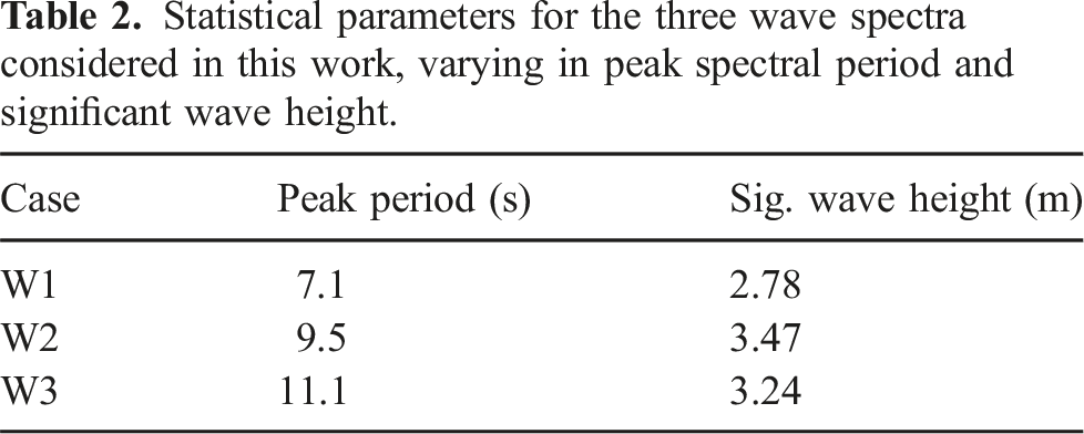
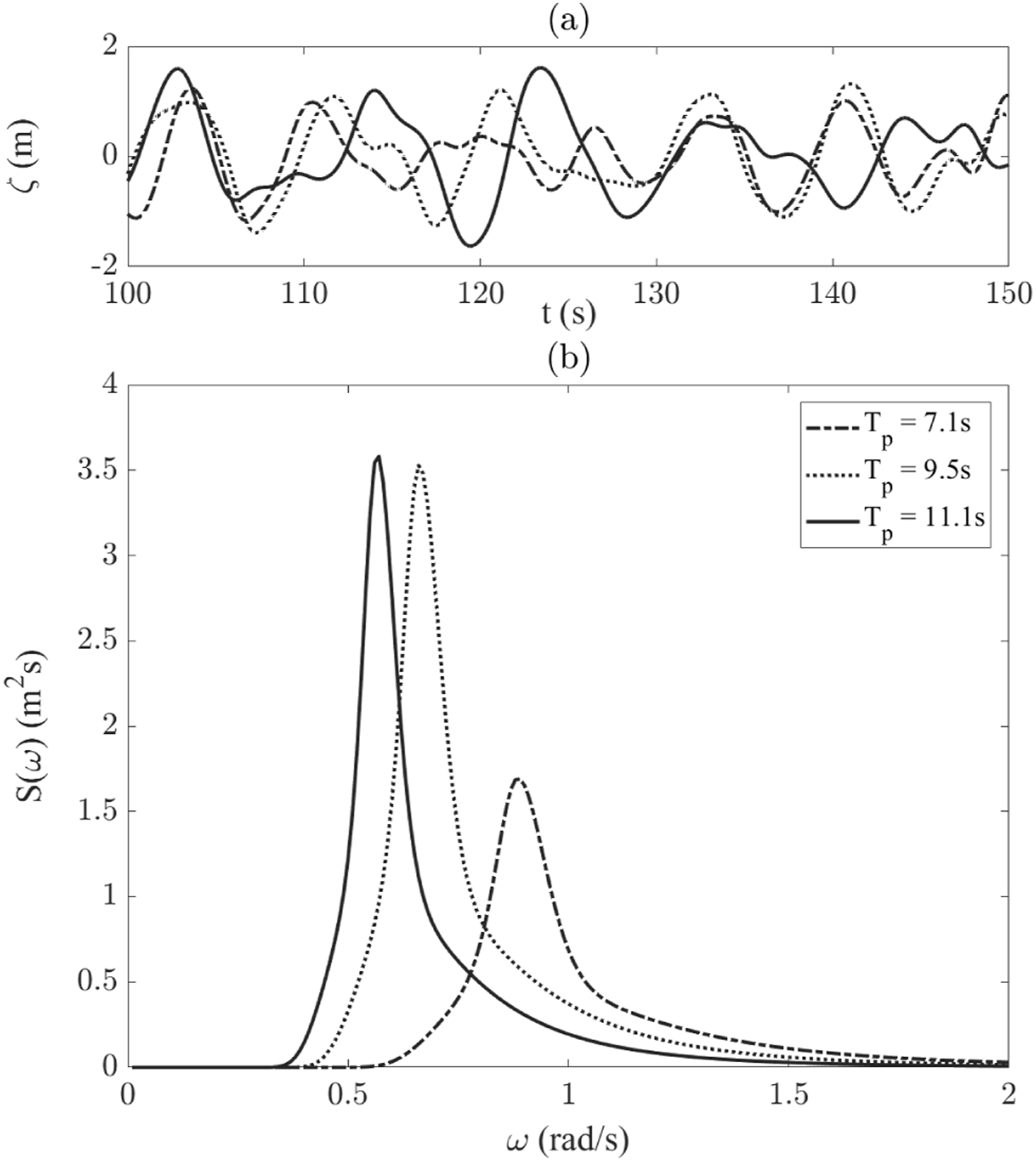
The three different spectra tested in this work, each following the JONSWAP description in equation (19).

5.2. Vehicle specifications and thrust allocation

The vehicle used in this study is the BlueROV2-Heavy, whose geometric and hydrodynamic parameters are given in Table 3 whilst the control parameters are given in Table 4. Remaining hydrodynamic parameters which were unavailable from literature, such as $X_{\dot{q}}$ and $M_{\dot{u}}$ were evaluated numerically using the potential flow solver WAMIT©.

Table 3.

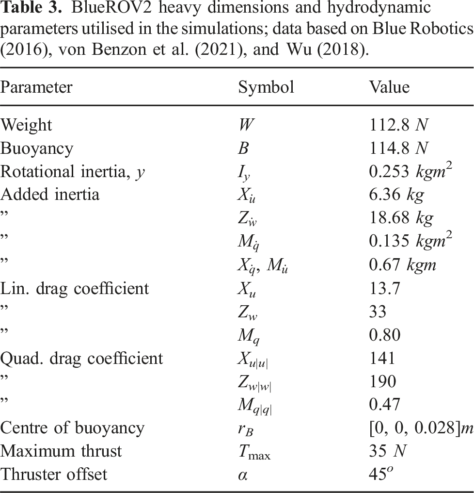
BlueROV2 heavy dimensions and hydrodynamic parameters utilised in the simulations; data based on Blue Robotics (2016), von Benzon et al. (2021), and Wu (2018).

Parameter	Symbol	Value
Weight	W	112.8 N
Buoyancy	B	114.8 N
Rotational inertia, y	I y	0.253 kgm2
Added inertia	$X_{\dot{u}}$	6.36 kg
”	$Z_{\dot{w}}$	18.68 kg
”	$M_{\dot{q}}$	0.135 kgm2
”	$X_{\dot{q}}$ , $M_{\dot{u}}$	0.67 kgm
Lin. drag coefficient	X u	13.7
”	Z w	33
”	M q	0.80
Quad. drag coefficient	X u|u|	141
”	Z w|w|	190
”	M q|q|	0.47
Centre of buoyancy	r B	[0, 0, 0.028]m
Maximum thrust	T max	35 N
Thruster offset	α	45 o

Table 4.

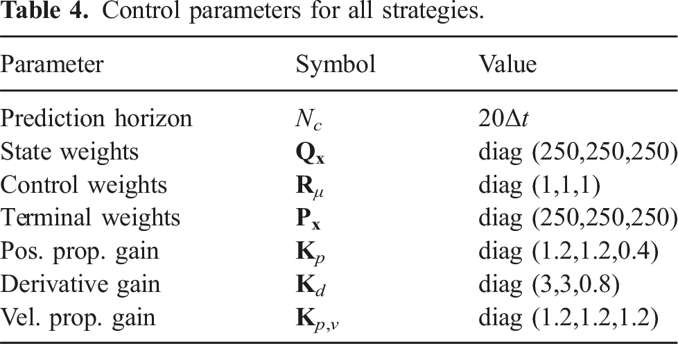
Control parameters for all strategies.

Parameter	Symbol	Value
Prediction horizon	N c	20Δt
State weights	Q x	diag (250,250,250)
Control weights	R μ	diag (1,1,1)
Terminal weights	P x	diag (250,250,250)
Pos. prop. gain	K p	diag (1.2,1.2,0.4)
Derivative gain	K d	diag (3,3,0.8)
Vel. prop. gain	K p,v	diag (1.2,1.2,1.2)

The BlueROV2-Heavy is controllable in all Do through an array of eight thrusters. The control vector is therefore $\mathit{\mu }={[{\mu }_1,{\mu }_2,{\mu }_3,{\mu }_4,{\mu }_5,{\mu }_6,{\mu }_7,{\mu }_8]}^T$ where μ₁ − μ₄ relate to the horizontal thrusters whilst μ₅ − μ₈ relate to the vertical thrusters, the former featuring an angular offset, α.

Property 5.1

The controller inputs are normalised and bounded such that −1 ≤ μ _i ≤ 1, which relate to the extreme limits of the thruster capability.

An affine model is adopted (Fossen, 1994), adjusted to include a first order response term to represent the inherent time-delay in the system between the control input command and the produced torque from the motors. The contributions from propulsive forces in the vehicle local-frame are defined as:

$\mathit{\tau }=\left(1-e^{-t/t_m}\right){\mathit{B}}_{\mathit{\mu }}{\mathbf{K}}_{\tau }\mathit{\mu }$

(35)

where t _m and t represent the motor time constant and surpassed time, respectively, and B _μ is the thrust allocation matrix, defined explicitly in Appendix 6. Also, ${\mathbf{K}}_{\tau }=\text{diag}(T_{\mathit{max}})\in {\mathbb{R}}^{8\times 8}$ is a force co-efficient matrix describing the capability of the thrusters where T _max = 35N is the maximum force producible per thruster.

5.3. Baseline controllers

To analyse the performance of the proposed framework, the NMPC with DSWP was compared against three baseline controllers: a cascaded position-velocity PD controller (referred to as C-PD from henceforth), a NMPC controller which does not include the wave disturbance preview information in the optimisation of the control actions (referred to as NMPC-B from henceforth) and a cascaded position-velocity PD with feed-forward (FF) controller (referred to as FF from henceforth). The first two are to provide a basic reference against controllers with no wave disturbance knowledge, with the latter incorporating the prediction algorithm to calculate disturbance compensating control actions but without an optimisation stage on the control trajectory. The NMPC-B architecture is considered “blind” with respect to wave-induced disturbances and this is effectively equivalent to the control anticipating ${\tilde{\mathit{\tau }}}_E=0$ . With reference to Table 4, all parameters were tuned heuristically with the NMPC parameters obtained by consideration of Bryson’s rule (Bryson and Ho, 1975) as a first approximation, subsequently refining values accordingly. Throughout the study, the comparative analysis focuses on the two predictive control schemes as these both incorporated the DSWP algorithm and thus are of more interest in terms of performance.

All controllers need to simultaneously control the heave and pitch through the same set of thrusters. To this end, a control allocation algorithm similar to that detailed in (Fossen, 2011) is employed using an inverse approach. This simplifies the control strategy by calculation of generalised control actions ${\mathit{\mu }}_g\in {\mathbb{R}}^3$ and producing a solution for $\mathit{\mu }\in {\mathbb{R}}^8$ . Considering equation (35), the control vector is determined through:

$\mathit{\mu }=\left[\left(1-e^{-\mathrm{\Delta }t/t_m}\right){\mathbf{K}}_{\mathit{\tau }}^{-1}\right]{\mathit{B}}_{\mathit{\mu }}^{†}\mathit{\tau }$

(36)

where ${\mathit{B}}_{\mathit{\mu }}^{†}$ is the Moore-Penrose pseudo-inverse of B _μ and τ = τ _max ⊙ μ _g where ${\mathit{\tau }}_{\mathit{max}}\in {\mathbb{R}}^3$ is the maximum force or moment producible in each DoF. Calculation of the generalised control input μ _g for the PD controller and FF controller is therefore defined as:

${\mathit{\mu }}_{PD}={\mathbf{K}}_{p,v}\left[\left({\mathbf{K}}_p\mathbf{e}+{\mathbf{K}}_d\dot{\mathbf{e}}\right)-\mathit{\nu }\right]$

(37)

${\mathit{\mu }}_{FF}={\mathit{\mu }}_{PD}+{\mathit{\tau }}_{\mathit{max}}^{-1}\odot \left({\mathbf{M}}_{\mathbf{A}}\dot{{\mathit{\nu }}_{\mathbf{p}}}+\mathbf{D}({\mathit{\nu }}_p){\mathit{\nu }}_p\right)$

(38)

where $\mathbf{e}={\mathbf{x}}_r-{\widehat{\mathbf{x}}}_k$ is the proportional error between the set-point reference and estimated state, with each controller exploiting the EKF as a state estimator to account for sensor noise across all tests.

5.4. Station keeping accuracy

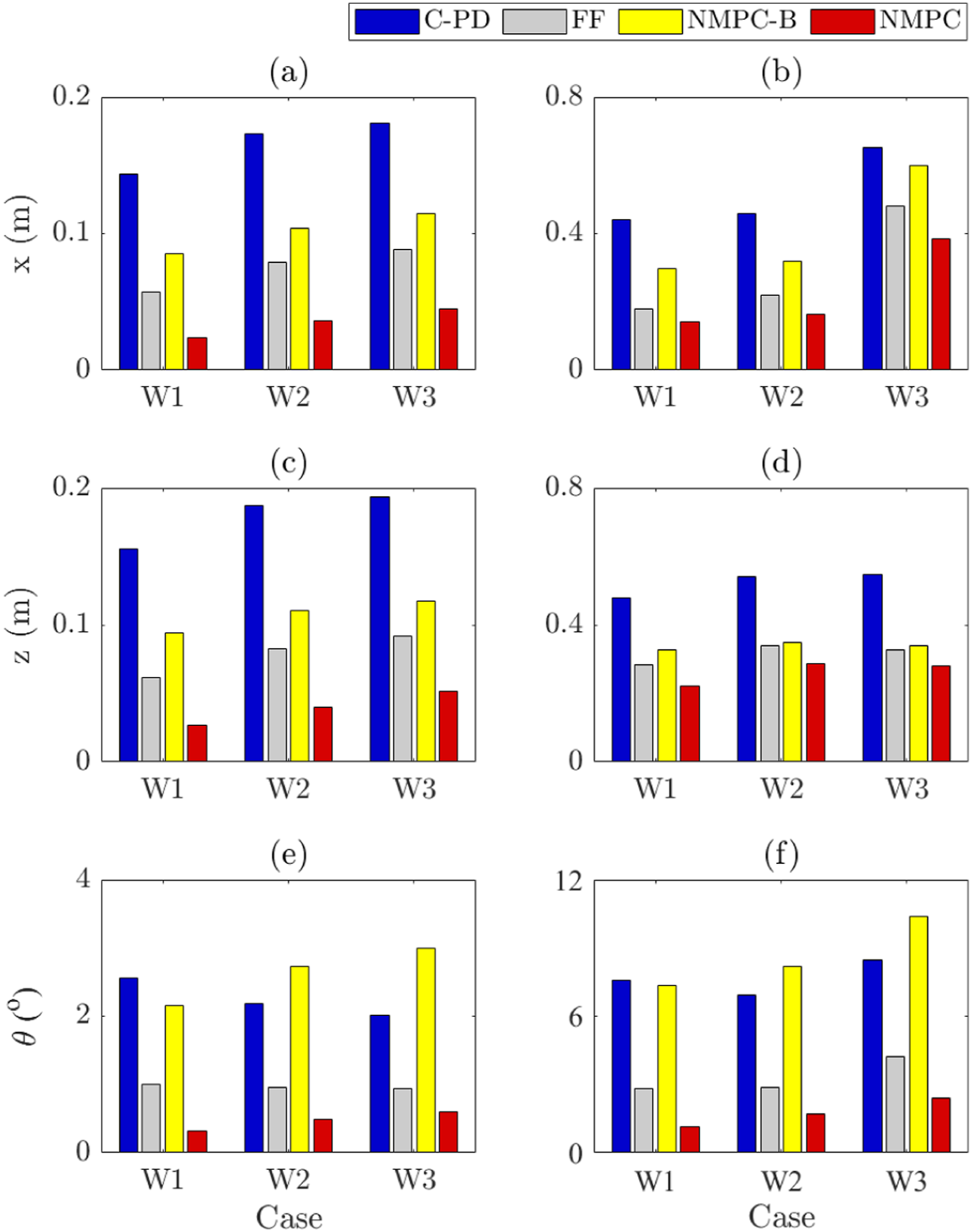
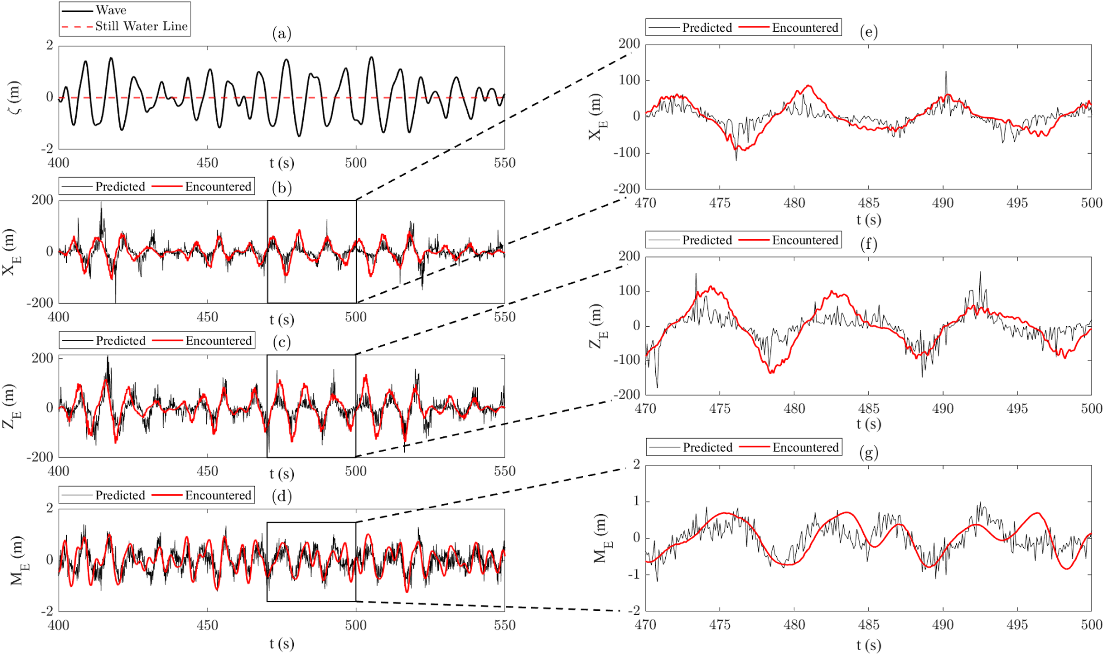
Initial performance analysis focused on the comparative performance against the three baseline controllers with minimal uncertainty in the system. Throughout these tests, only noise arising from sensor measurements was considered (inclusive of both wave elevation and state). A Gaussian filter was applied to the wave height measurements, whilst the EKF was utilised to reduce the uncertainty associated with the state measurements and produce the full-state vector. For all cases and DoF, the RMSE was analysed along with the maximum error that was recorded throughout the entire temporal segment for reference; an example case is displayed in Figure 8 with quantitative results given in Figure 9.

Figure 8.

Temporal segment of the station keeping simulation (b–d) subject to the wave profile shown in (a) and the associated enlargement (e–g), showing the positional evolution for case W2. Here, the reference state is defined as x _r = [50, − 5, 0] in the global frame and the model is assumed to be accurate; measurement noise is still considered.

Figure 9.

(a, c, e) RMSE and (b, d, f) maximum error observed for each DoF and sea state considered for the station keeping mission where only sensor noise is considered and zero additional spectral noise is present.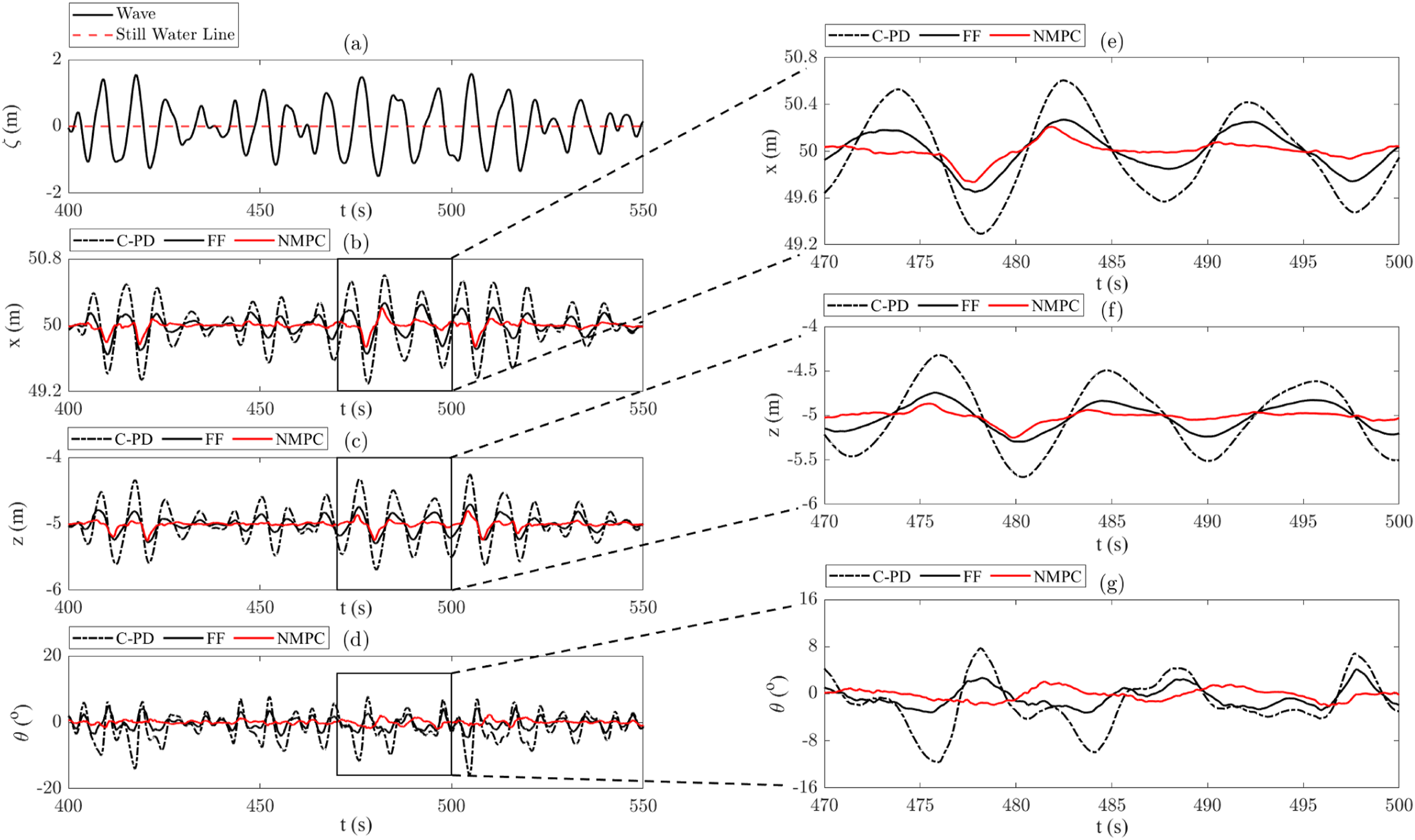

As anticipated, the NMPC method produces the lowest values for both RMSE and maximum error, however it was noted that the disparity in maximum error was much lower with some instances returning only $\approx 14\%$ improvement over the FF method (heave, case W3). For the surge and heave, a mean improvement in RMSE of $\approx 52\%$ was witnessed between the NMPC and FF methods, whilst the pitch RMSE was reduced by $\approx 51.5\%$ showing consistent improvements irrespective of DoF. With respect to maximum error, the mean improvement was lower at $\approx 19.5\%$ and $\approx 48\%$ for the linear and angular motions, respectively, still showing fair improvements particularly for the pitch. Although maximum errors of up to 0.38m were witnessed even for the NMPC method (Case W3), these only occur at short time intervals across the entire mission, supported by the low RMSE error observed. Notably, the NMPC-B method clearly offers vast improvement over a standard feedback controller (in positional regulation) but fails to mitigate the effects of wave disturbances effectively, with the FF method outperforming in all DoF and wave cases.

Interestingly, the NMPC-B struggled to handle pitch disturbances and was even outperformed by the C-PD strategy. It is postulated that this arises due to the NMPC optimising control actions whilst accounting for restoring forces in the vehicle dynamics, thus less aggressive action is commanded without the knowledge that further impending disturbances are on the horizon. In contrast, the C-PD and FF methods are simply taking the most aggressive action (relative to the controller tuning) in order to regulate the state, irrespective of vehicle dynamics. Similarly, the coupling which exists between the surge and pitch likely contributes to greater pitch displacement, with the NMPC-B strategy requiring more aggressive corrective actions from greater displacements, thus negatively impacting the pitch as a result. A further interesting observation was that the pitch displacement remained low even when using the C-PD method, with a maximum value of 8.47 ^o recorded. The vehicle is naturally restoring at θ = 0 ^o , so the control required to minimise displacement can be less aggressive. The advantage of this is the potential to reduce the computational overhead of the control by only applying a predictive method to the lateral motions, using a typical feedback controller specifically for the pitch plane to reduce the angular displacement sufficiently. This would allow quicker convergence during the optimisation stage and thus assist with applicability to real-time applications.

Finally, Figure 10 displays a violin plot of each test case. This shows the distribution of the data by using a relative width proportional to the frequency of data points, therefore represents the frequency that the vehicle undergoes different positional errors. From this, the ability of the NMPC to constrain the vehicle motion to remain largely within a narrow band of positional error is clear, owing to the shorter and wider plots in all cases and all DoF. Particularly for the surge and heave, the variation in positional error is reduced significantly, in conjunction with the maximum error as previously mentioned. Even when adopting the FF strategy, the frequency of data points recorded in the vicinity of the reference position is clearly apparent, demonstrating that the predicted disturbances are being mitigated effectively.

Figure 10.

Violin plot highlighting the frequency density of positional error with respect to each wave case and control strategy.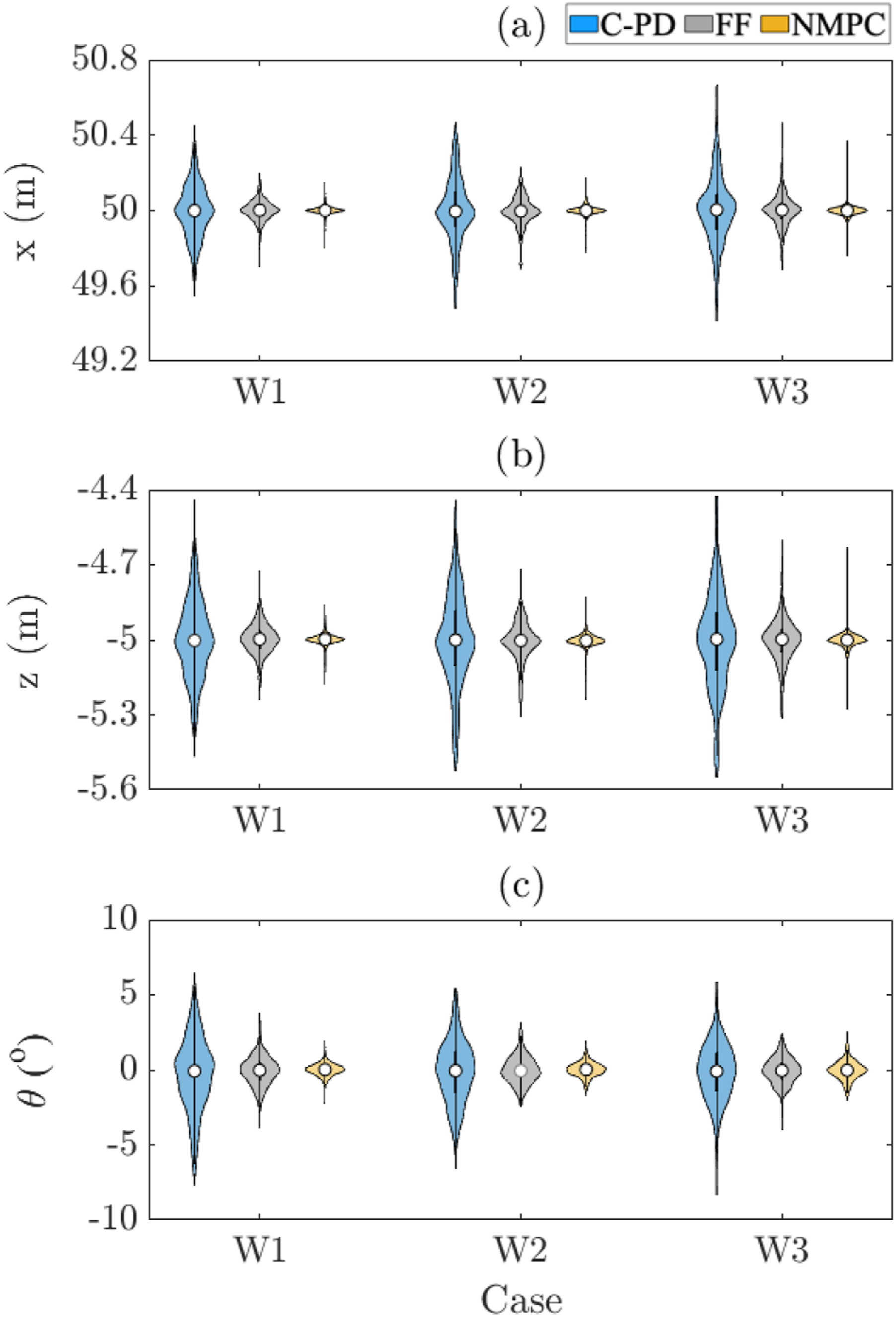

5.5. Sensitivity to noise

The effectiveness of predictive disturbance rejection is largely postulated on the accuracy of the wave disturbance preview. Any source of noise in the wave estimation, either deriving from inaccurate sensor readings at the measurement site or the occurrence of interference at the prediction site will intuitively affect the performance of the controller. To address the degree of robustness of the proposed methodology, we test the control performance under various degree of signal-to-noise ratio (SNR) on the output parameters of the wave predictor. Gaussian noise was directly injected to the output amplitude and phase of the DSWP inferred spectral components, simulating the conditions where predicted and encountered wave disturbances differ. The cases covered in this analysis involved SNRs of 5, 10 and 15. Figure 11 demonstrates how these levels of SNR affect the interpreted waveform by the controller against the wave experienced by the vehicle. Similarly, the effect of SNR levels on the predicted wave loading experienced by the vehicle compared to those actually encountered is shown in Figure 12.

Figure 11.

Spectral noise influence on the real versus interpreted wave. Ground truth refers to the wave (case W3) experienced by the vehicle, where-as the other displayed waves are what the controller interprets when including spectral noise.

Figure 12.

Temporal segment of the estimated loads during the station keeping simulation (b–d) subject to the wave profile shown in (a) and the associated enlargement (e–g), showing the evolution for case W2 with SNR₁₀ of spectral noise, showing how the estimated loads vary with added uncertainty.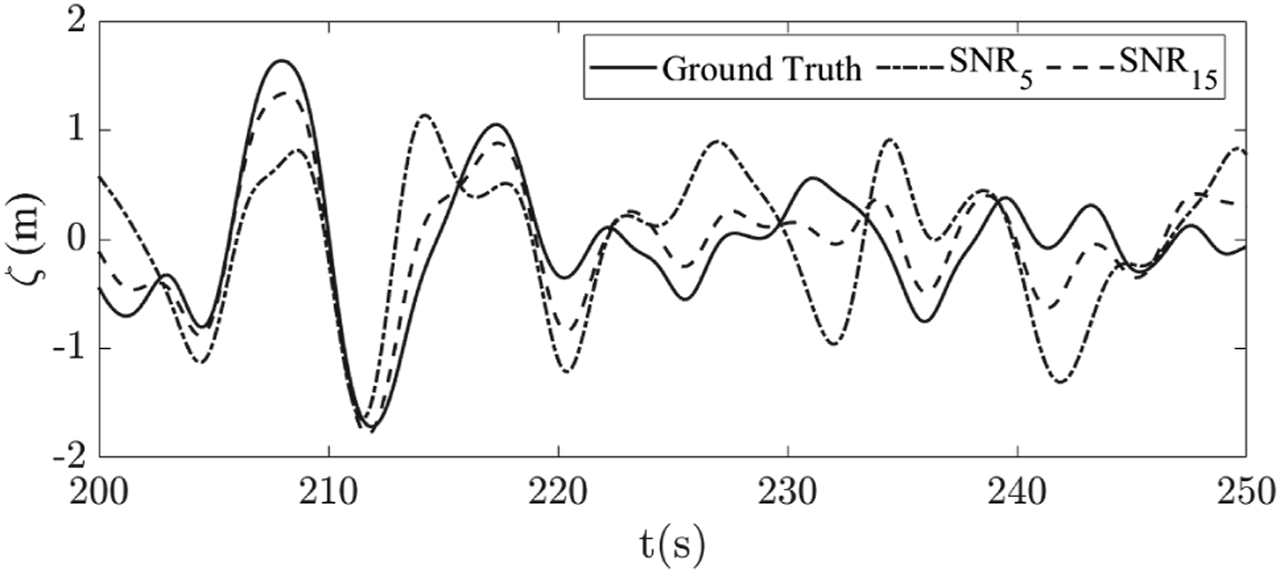

Station keeping performance under the three levels of SNR are shown in Figure 13, respectively, for the FF and NMPC controllers, also depicting the NMPC-B results to act as a reference. For almost all cases the NMPC outperforms the FF, with the only exception being the pitch control subject to large spectral noise, cases W2 and W3 in Figure 13(g). This is likely due to the fact the vehicle pitch is easily influenced by control actions, thus is more susceptible to unwanted motions if the predictions are not reasonably accurate. This being said, the pitch RMSE never exceeds 2 ^o and so this difference is irrelevant when considering the broader goal. In the surge and heave DoF, a mean reduction across all cases of $\approx 41\%$ in RMSE between the FF and NMPC schemes was witnessed, showing that even in the presence of significant spectral noise the inclusion of the optimisation step greatly increases station keeping performance. A key observation to raise with reference to the NMPC-B results is that the FF controller outperforms in the majority of cases, with only large levels of spectral noise causing worse state regulation performance. Given that the NMPC-B still features an optimisation loop, this finding demonstrates that knowledge of oncoming wave disturbances is critical in these scenarios for achieving high accuracy control.

Figure 13.

RMSE error for each DoF and sea state considered when different levels of spectral noise are considered, showing results for (a, d, g) SNR₅, (b, e, h) SNR₁₀ and (c, f, i) SNR₁₅ and the comparison between the FF and NMPC alongside the NMPC-B providing a baseline reference.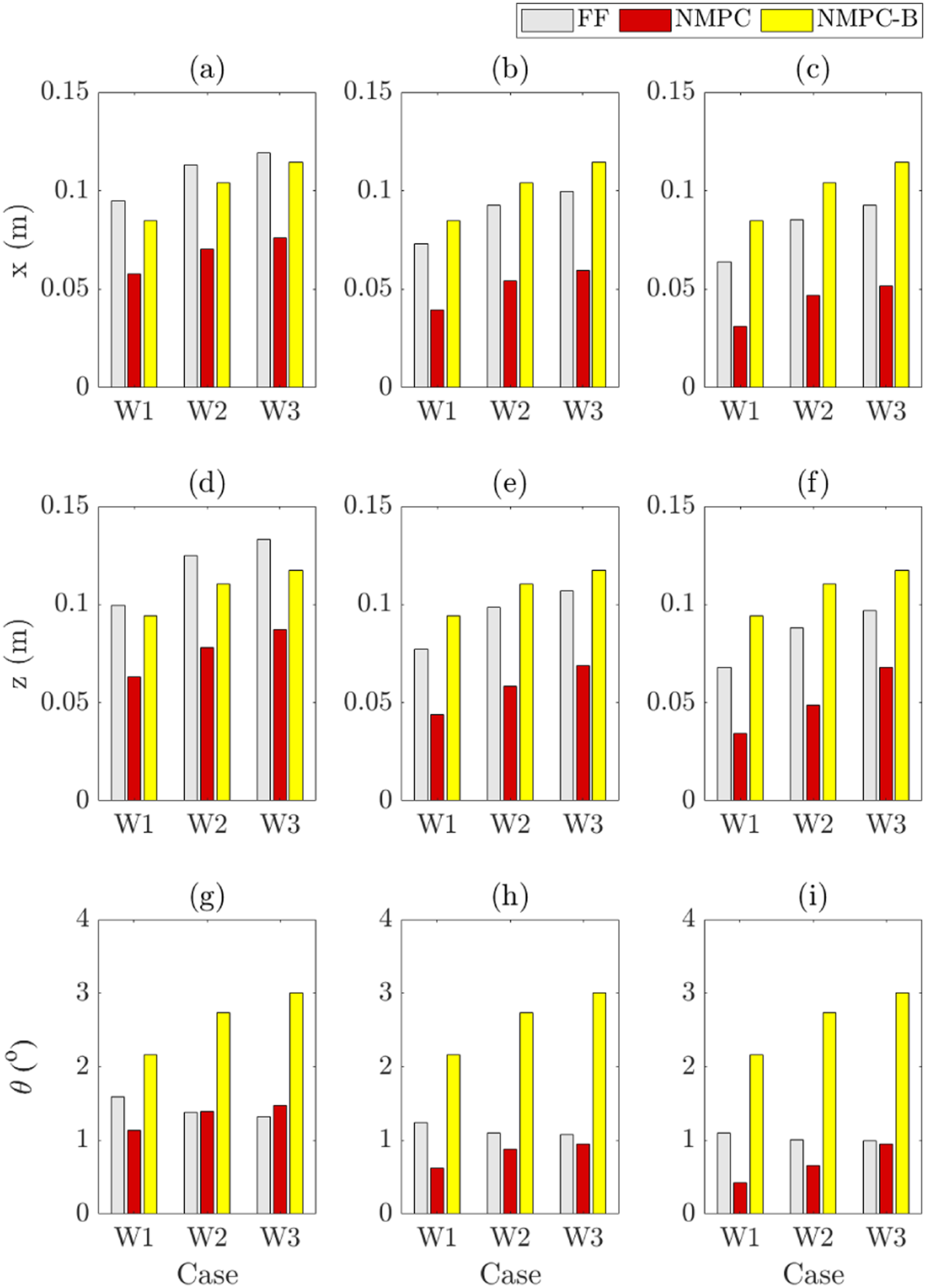

With reference to the cases presented in Section 5.4, the largest increase in RMSE when considering a non-ideal prediction was $\approx 19.5\%$ and $\approx 51\%$ for the linear and angular motions, respectively. It is key to note here that the absolute values of pitch displacement are minimal, thus even though the spectral noise had a significant effect, in absolute terms the station keeping accuracy is still high. These findings demonstrate that the inclusion of even relatively coarse predictions can improve performance substantially, with the inclusion of an optimisation stage over a horizon improving this further. This statement is supported even further by the fact the NMPC-B scheme rarely offers greater performance than the FF method (only the SNR₅ cases show worse state regulation), and the NMPC scheme exploits even the coarsest wave estimations to good effect to improve set-point regulation capabilities. It is worth noting that in these cases the EKF is producing an accurate estimation of the vehicle state, but for operations with high speeds and high nonlinear effects a UKF may be more applicable, as noted in (Allotta et al., 2015).

The improved performance of NMPC often results in a trade-off of increased power consumption, further magnified in highly unsteady scenarios and (potentially) noisy predictions as in the cases examined here. To evaluate the power expenditure of the proposed control architecture, the integral power output during the station keeping tasks was estimated for the C-PD, the FF and the NMPC. Exploiting data provided by the manufacturer (Blue Robotics, 2016), the power at a nominal operating voltage of 16V was approximated as:

$P_{\tau }=\sum _{i=1}^{3}0.0011{\tau }_i^3+0.02078{\tau }_i^2+0.297{\tau }_i$

(39)

where P _τ is the total power consumed by the generalised control actions, where i refers to the DoF (x, z, θ). Neglecting hotel load contributions, the cumulative power over the entire mission was evaluated as a time-averaged summation and these results are given in Table 5.

Table 5.

Power consumed during the station keeping mission for each wave case and control strategy when the spectral components are perturbed by varying levels of noise. As the C-PD controller does not use the disturbance preview this only features in the SNR₀ case.

Case	Controller	Power consumed (W)
		SNR0	SNR5	SNR10	SNR15
W1	C-PD	17.14	—	—	—
	FF	38.51	45.45	40.75	38.23
	NMPC-B	26.99	—	—	—
	NMPC	52.21	87.83	70.66	58.80
W2	C-PD	23.80	—	—	—
	FF	47.08	52.04	46.78	46.13
	NMPC-B	36.49	—	—	—
	NMPC	56.49	99.36	77.80	62.15
W3	C-PD	20.59	—	—	—
	FF	37.83	47.56	40.93	38.94
	NMPC-B	28.47	—	—	—
	NMPC	47.98	88.9	74.73	57.55

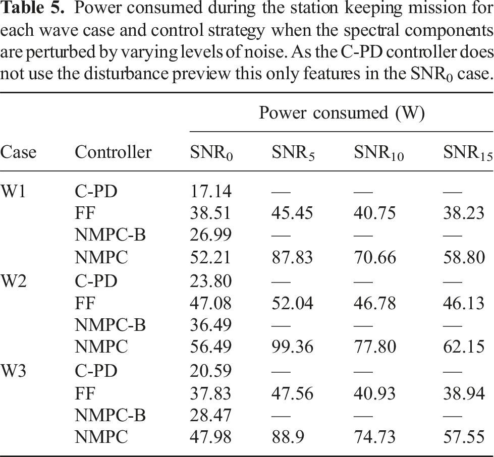
Considering the case SNR₀ where the uncertainty considered is purely attributed to sensors (state and wave elevation), the relative increase in performance surpassed the relative increase in power consumption for all cases. A mean increase of $\approx 27.5\%$ coincided with a mean reduction of linear station keeping error of $\approx 52\%$ , whilst also reducing the pitch error by $\approx 51.5\%$ indicating that the additional energy required is utilised to good effect. As expected, the consumed power increases with increasing spectral noise, however the increase is much sharper for the NMPC method, likely attributed to the controller iterative optimisation stage over the one-step estimated control action produced by the FF scheme. For high spectral noise, the power consumed by the NMPC method was almost double of the FF method for case W2, showing a much higher dependence on accurate disturbance predictions to efficiently consume power. Between the cases for SNR₅ and SNR₁₅, the power consumed increased by $\approx 54.5\%$ for the NMPC, whilst only an increase of $\approx 18\%$ was witnessed for the FF cases, again supporting the previous hypothesis relating to the optimisation stage.

5.6. Sensitivity to communications delay

A key factor in deploying this control methodology is establishing a communication network between the wave buoy and the vehicle to pass the information pertaining to oncoming wave disturbances. As alluded to in Section 1, this can be performed two ways: either by (1) transmitting this data through air over a wireless link from the buoy to a base station, before relaying this to the vehicle via a tether, or (2) directly to the vehicle through water over a wireless link, meaning the vehicle can operate untethered. Using method (1) has the major advantage of very little latency, seen as wireless communications in air is an extremely well established field and a wired connection to the vehicle (over ethernet for the BlueROV2) means latency will be minimal. The drawback is that the vehicle is restricted by the length of the tether, so ultimately this limits the operational range from the base station. Alternatively, method (2) removes this restriction by operating untethered, but incurs the well-known limitation of wireless underwater communications which are often slow and suffer from increased attenuation and bandwidth limitations. It is therefore critical that these effects are analysed to demonstrate this control methodology can be implemented with confidence in a real environment.

Firstly, consider that the measured wave-height record (ζ _M ) is analysed at the wave-buoy and the data to be transmitted are sets of spectral parameters, (A, ω, ϵ). For the wave cases analysed in this work, these vary from 80 to 100 sets of parameters after thresholding. If each value of (A, ω, ϵ) is considered to be of data-type 32-bit float (8 bytes) and we analyse the 100 components case with three parameters per component, then the amount of data requiring transmission would be 9600 bits. To calculate the full transmission time, consideration of the transmission distance along with propagation speed need to be accounted for, as well as inclusion of some overheads introduced by the transmission protocol; these overheads usually amount to $\approx 10\%$ (Goldsmith, 2005).

For wireless transmission in air, a standard offshore WiFi network can range over hundreds of meters and operates in the Mbps range at minimum (Chen et al., 2021). Considering the 50m transmission distance specified throughout our previous analysis, this implies a maximum transmission time of $\approx 0.02$ s, effectively real-time communication, even when including overheads introduced by wireless transmission. This makes this option attractive, despite the necessity for a tether. Eradicating the reliance of a tether, on the other hand, requires consideration of underwater wireless communications.

Wireless transmission in water is far slower than air, stemming from the density of sea water, which implies that much lower frequencies are required to reduce signal attenuation and improve range. However, commercially available underwater modems can still transmit at rates of 30kbps for up to 1000m (NOAA, Revised 2022); this would imply a transmission time for the data alone of $\approx 0.32$ s. Acoustics travel at a speed of 1500m/s in water, so over 50m the approximate propagation delay would be $\approx 0.03$ s, which inclusive of 10% overheads implies a total transmission time of $\approx 0.35$ s. This can be reduced by using well established lossless compression methods. This value reflects the maximum permissible update rate of the disturbance prediction and thus also the minimum length of the predictable region required to always have a disturbance prediction available to the controller; the results in Section 3.2 with prediction lengths of $\approx 2$ s prove this is viable. In a real-world setting it is unlikely that direct underwater communication would be favoured given these additional considerations and the exacerbated losses due to scattering.

However, there is optimism that underwater communications are vastly improving, as evidenced by recent demonstration of successful underwater data transmission at 1Mbps over a 300m range in shallow waters (NTT, 2022). This speed of transmission relates to a delay of only $\approx 0.02$ s, aligning it with the lower-end speeds of a WiFi connection and near real time, thus potentially providing a solution for untethered, direct underwater communication between the wave buoy and the vehicle. The evidence that high speed underwater communications over shorter ranges could become commercially available in the near future offers confidence that a control methodology like the one detailed in this work could indeed become viable.

Regardless of the communication strategy, transmission from the measurement point to the vehicle is likely to expose the disturbance preview to a temporal delay. This is reflected in the disturbance prediction potentially being misaligned with the actual disturbance. To address this, the following analysis delves into the effect of time delays when estimating the wave-induced disturbances, investigating how the control performance of the FF and NMPC methods are affected by varying degree of delay. In these tests, the disturbance estimation is considered to be accurate, that is, SNR=0, but the controller predicts the disturbance to occur after it has arrived at the vehicle location (see Figure 14). Constant time delays of 0.25s and 0.5s are tested, along with a case where the time delay is varied randomly (uniform distribution) during the simulation between 0 and 1s. This additional case aims to simulate communication instabilities that may be caused by changing environmental conditions. As this final case deals with a randomly generated delay at each time-step, the results from these tests were averaged over three repetitions. These test cases were selected on the basis that it is already commercially viable to achieve stable communications with time delays of $<$ 1s, as discussed earlier.

Figure 14.

Time delay influence on the real versus interpreted wave. t _d = 0s refers to the wave (case W3) experienced by the vehicle, whereas the other displayed waves are what the controller interprets when including a time delay.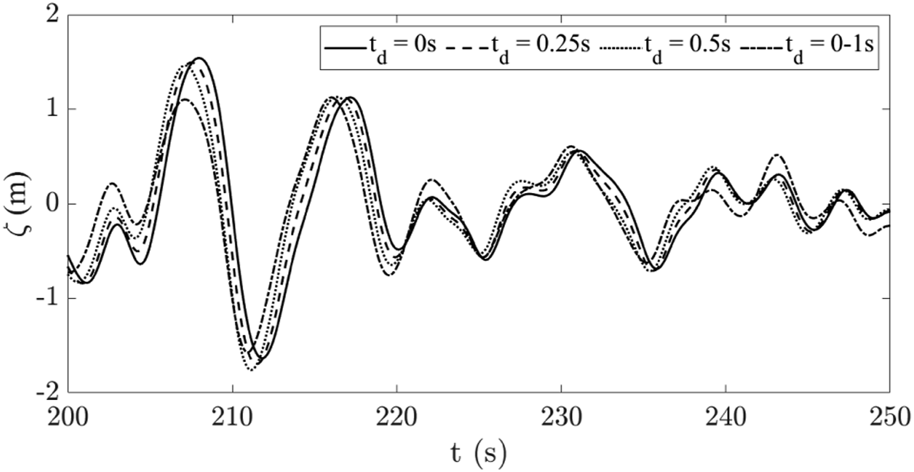

As can be seen in Figure 15 and comparing to Figure 9, unsurprisingly there is an increase in RMSE for all degrees of freedom. However, even with this increase, the NMPC inclusive of disturbance time delay still outperforms the blind NMPC, supporting the claims in the previous section that disturbances with some level on inaccuracies can still be exploited to improve control performance. For all cases, a mean increase in RMSE of $\approx 60\%$ , $\approx 59\%$ , $\approx 48\%$ was witnessed for the surge, heave and pitch, respectively, when using an NMPC with no disturbance estimations compared to instances with time delay. The largest error is related to the case where t _d was varied between 0 and 1s randomly, owing to the constantly varying magnitude of online corrections required by the controller.

Figure 15.

RMSE error for each DoF and sea state considered when different levels of spectral noise are considered, showing results for (a, d, g) t _d = 0.25s, (b, e, h) t _d = 0.5s, and (c, f, i) t _d = [0, …, 1]s and the comparison between the FF and NMPC alongside the NMPC-B providing a baseline reference.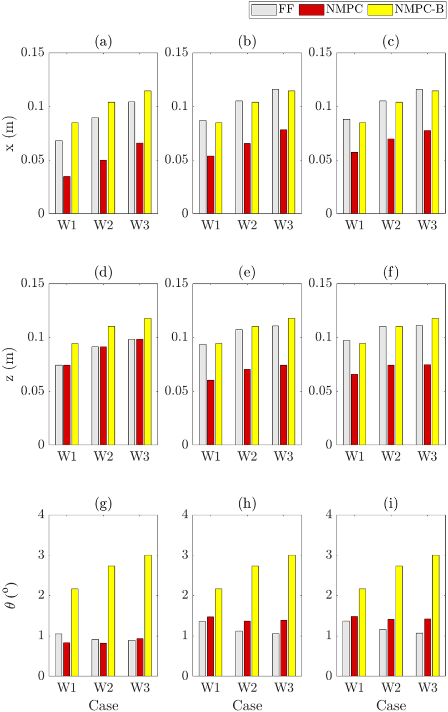

These results show a remarkable level of robustness of the controller to realistic communication delays. In particular, a dependency on the characteristic time scale of the wave is observed, confirming that longer wavelengths exhibit less degradation on control performance caused by time delays. This is motivated by longer wavelengths being associated with shallower gradients in the magnitude of the temporal disturbance. The fact that, in real-world sea climates, the wave period is typically much longer then the time-delay suggests that the degradation in control performance for the strategy proposed should remain consistent with that caused by a noisy signal, Section 5.5.

6. Conclusions

In this article, a method for the predictive disturbance mitigation of ocean waves has been proposed for underwater vehicles, utilising real-time, recursive preview information of future disturbances derived through the inclusion of a wave predictor. With regards to the wave predictor, an experimental study focusing on short-term short-distance predictions returned a maximum RMSE of 0.045m over a 2 s wave prediction, validating applicability for use within a predictive control architecture which can be confidently extended to larger distances and prediction intervals. Upon embedding the wave predictor within two different predictive control methods analysed (FF and NMPC), both were shown to effectively reduce the positional error of the vehicle, with the latter showing a mean improvement of 52% in comparison to the former due to the inclusion of an optimisation of future control actions. Performance improvements were demonstrated in the presence of various sources of noise and uncertainty, including time delays in the disturbance prediction, highlighting the robustness of the system to any mismatch between the predicted disturbances and those encountered by the vehicle. Ultimately, these results provide evidence that predictive control, once supported by a robust disturbance predictor, can indeed represent a solution to the current limitations associated with the employment of autonomous vehicles in hazardous ocean climates, enabling more complex navigation (Walker and Giorgio-Serchi, 2023) and manipulation (Walker et al., 2024) tasks and facilitating their uptake in a broader range of offshore operations.

Supplemental Material