Sage Journals: Discover world-class research

Abstract

Recent progress in semantic scene understanding has primarily been enabled by the availability of semantically annotated bi-modal (camera and LiDAR) datasets in urban environments. However, such annotated datasets are also needed for natural, unstructured environments to enable semantic perception for applications, including conservation, search and rescue, environment monitoring, and agricultural automation. Therefore, we introduce WildScenes, a bi-modal benchmark dataset consisting of multiple large-scale, sequential traversals in natural environments, including semantic annotations in high-resolution 2D images and dense 3D LiDAR point clouds, and accurate 6-DoF pose information. The data is (1) trajectory-centric with accurate localization and globally aligned point clouds, (2) calibrated and synchronized to support bi-modal training and inference, and (3) containing different natural environments over 6 months to support research on domain adaptation. Our 3D semantic labels are obtained via an efficient, automated process that transfers the human-annotated 2D labels from multiple views into 3D point cloud sequences, thus circumventing the need for expensive and time-consuming human annotation in 3D. We introduce benchmarks on 2D and 3D semantic segmentation and evaluate a variety of recent deep-learning techniques to demonstrate the challenges in semantic segmentation in natural environments. We propose train-val-test splits for standard benchmarks as well as domain adaptation benchmarks and utilize an automated split generation technique to ensure the balance of class label distributions. The WildScenes benchmark webpage is https://csiro-robotics.github.io/WildScenes, and the data is publicly available at https://data.csiro.au/collection/csiro:61541.

Keywords

Semantic scene understanding performance evaluation and benchmarking data sets for robotic vision data sets for robot learning

1. Introduction

For autonomous agents to operate beyond the structured and controlled environments of urban streets and warehouses, they require the ability to understand the natural world. Perception in natural environments consists of additional complexities as these environments generally contain highly irregular and unstructured elements, making them less predictable than structured environments. For robots to account for these complexities, they must perceive the environment at a fine-grained level. Fine-grained semantic scene understanding has enabled many applications in urban environments, including mapping, localization, object retrieval, and dynamic situational awareness. Research progress on these tasks has primarily been enabled by the availability of semantically annotated bi-modal (camera and LiDAR) datasets.

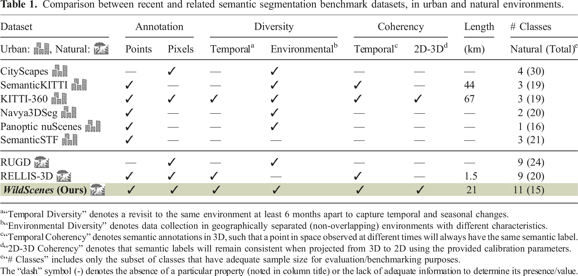
While there are many semantic segmentation datasets, most of them focus on structured environments such as outdoor urban areas (Behley et al. (2021); Cordts et al. (2016); Zhou et al. (2017)), or indoor environments (Silberman et al. (2012); Ruiz-Sarmiento et al. (2017)). Consequently, there is a need for more large-scale semantic segmentation datasets in unstructured, natural environments. These types of environments pose several challenges beyond those encountered in more structured environments. Firstly, in an urban environment, it is clear to define a building or a road, yet the separation between classes can be less defined in a natural environment. For example, the distinction between dirt and mud, or between grass and a shrub. Secondly, the density (or clutter) of natural environments causes boundary ambiguity to occur due to the co-occurring nature of natural semantic classes (e.g., tree leaves and trunks). These challenges make semantic segmentation incredibly challenging in these environments and make it all the more important for future research to focus on developing robust perception systems that can operate in these environments (Borges et al. (2022)).

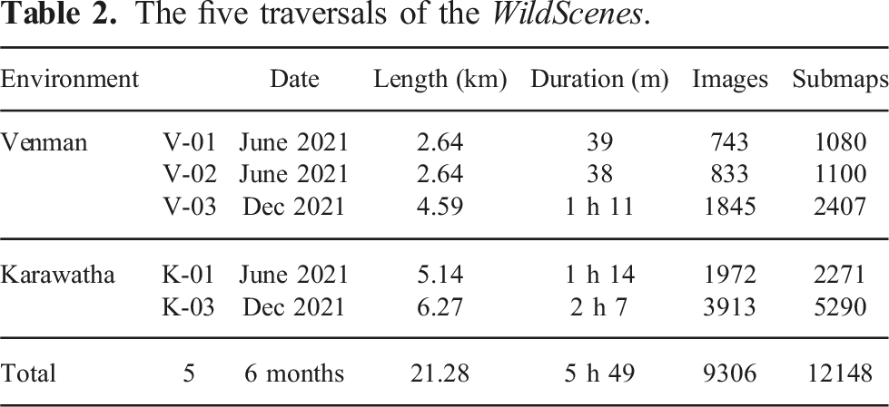
Therefore, we introduce WildScenes, a bi-modal benchmark containing 2D and 3D semantic annotations in natural environments. WildScenes comprises multiple sequential traverses through two distinct natural locations in Australia, including revisits after 6 months. This temporal and environmental diversity are essential properties for lifelong robotic applications to address the degradation in semantic inference that occurs due to either changes in environment or changes due to temporal and seasonal variations. WildScenes provides long-term sequential synchronized 2D image and 3D point cloud data, and we provide accurate 2D semantic labels via human annotation (refer to Figure 1).

Figure 1.

The WildScenes benchmark consists of five large-scale traversals in two natural forest environments—Venman (V-01, V-02, V-03) and Karawatha (K-01, K-03). In the center of the figure, the traversals from each environment are depicted using the corresponding semantically annotated 3D global map of that traversal. The zoom-in views of example locations with prominent semantic classes are depicted. For each class example, three images depicting the 2D image, 2D semantic annotation, and 3D semantic point cloud of corresponding location and viewpoint are provided.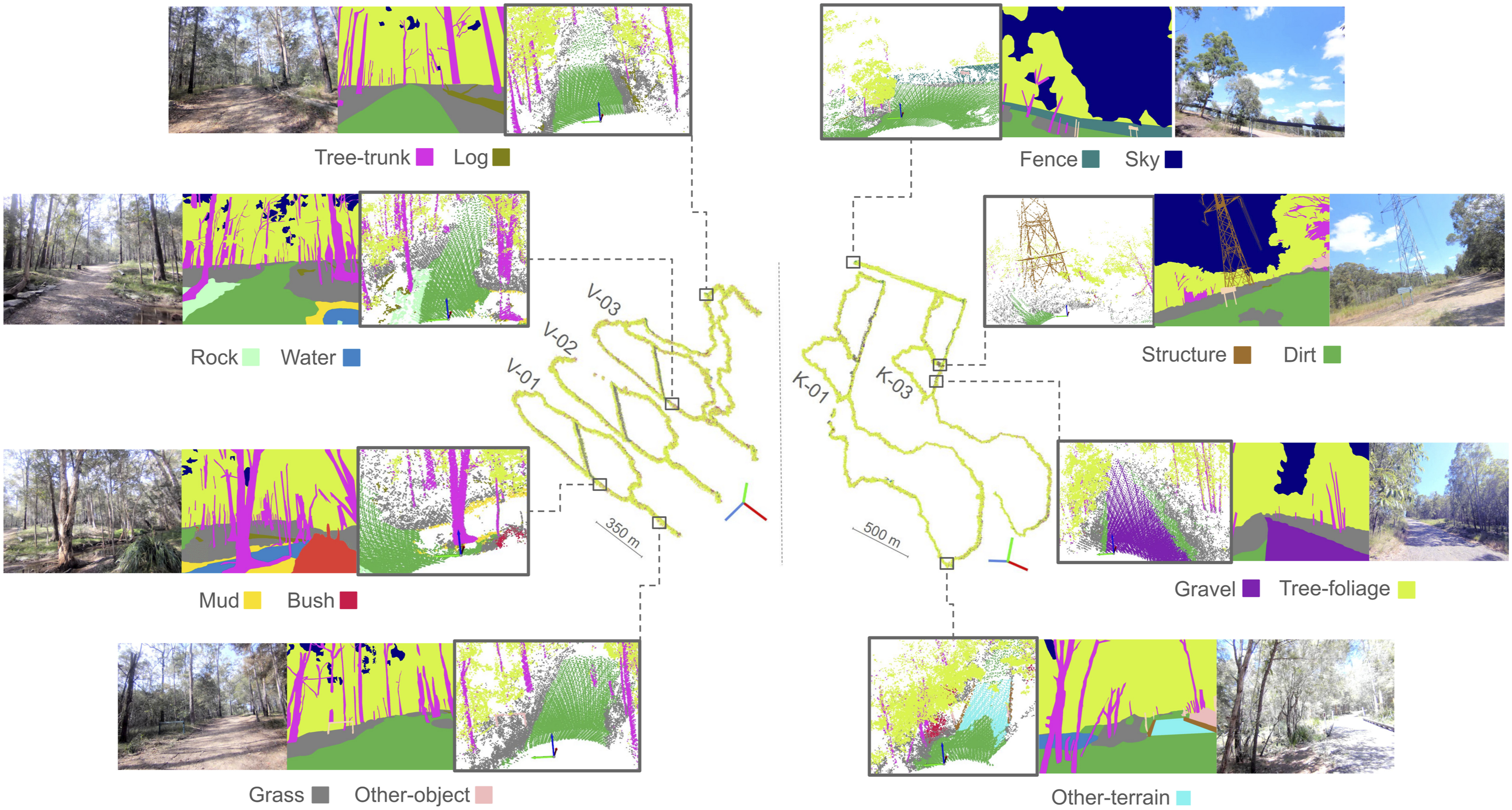

We also generate accurate 3D semantic point cloud labels using a LiDAR sensor along with significant post-processing. Our raw 3D data is generated using a spinning LiDAR sensor, which allows for a wide vertical field-of-view and is thus able to scan all objects in the environment, including tall trees. We then use a state-of-the-art LiDAR-inertial SLAM system to generate an accurate 6-DoF trajectory and a globally consistent point cloud map for each traversal. Utilizing the globally consistent map and trajectory combined with precisely calibrated extrinsics and intrinsics, we are then able to accurately transfer the 2D semantic annotations from multiple views into the 3D point clouds in a manner that enforces the temporal and 2D-3D coherence of semantic labels.

The main advantages of the WildScenes benchmark include: scale (over 20 km of sequential traversal over the course of 6 months), size (9,306 images and 12,148 point clouds), high 2D resolution (2016 × 1512), high 3D point density ( $>$ 70,000 points per cloud) and accurate 6-DOF localization information. We provide: (1) rectified RGB images with 2D semantic annotations by human annotators. (2) 3D LiDAR point clouds, with motion distortion correction and 3D semantic annotations generated via efficient 2D label transfer. (3) Label distributions for 3D points to represent the semantic ambiguity in natural environments.

Additionally, our benchmark dataset involves traversing through very dense and rough terrain, which could aid research on autonomous systems that need to operate in remote, difficult-to-access locations. To enable research on semantic domain adaptation in natural environments, we provide (1) traversals in geographically separated environments to capture a different sample distribution for each of our semantic classes and (2) repeat traversals in the same environment with a 6-month time gap to capture distribution shift due to temporal and seasonal changes. In summary:

• We introduce the WildScenes benchmark, which contains synchronized 2D and 3D sequential, dense semantic annotations of multiple large-scale traversals in unstructured natural environments.

• We provide a benchmark for semantic scene understanding in natural environments for 2D and 3D tasks. The benchmark contains train-val-test splits optimized to balance the class label distribution, including separate splits for domain adaptation downstream tasks.

• We provide a strategy for generating dense 3D labels without human annotators (named LabelCloud), utilizing geometric projection from 2D labeled images with a robust visibility check. Additionally, this method generates a histogram of label assignments per point, which could be used in uncertainty-aware semantic segmentation algorithms.

2. Related work

Semantic segmentation in 2D and 3D aims to assign pixel/point-wise labels for images and point clouds for scene understanding. There are many established datasets and learning-based methods developed for urban scene understanding, including SemanticKITTI (Behley et al. (2021)), Cityscapes (Cordts et al. (2016)), KITTI-360 (Liao et al. (2022)), Panoptic nuScenes (Fong et al. (2022)), Boreas (Burnett et al. (2023)), SemanticPOSS (Pan et al. (2020)), Rope3D (Ye et al. (2022)), Navya3DSeg (Almin et al. (2023a)) and SemanticSTF (Xiao et al. (2023)), with an overview of the most prominent semantic segmentation datasets provided in Table 1. These datasets focus mainly on applications and scenarios for autonomous driving in urban environments. A semantic understanding of the environment is key to path planning and navigation in natural environments, where traversability is dependent on a wealth of information beyond the 3D geometry of the scene. For example, a legged platform that could navigate a flat stretch of grass or dirt with ease could experience a catastrophic failure attempting to navigate a stretch of mud or sand. Furthermore, natural environments can also undergo significant changes over short periods of time, due to seasonal changes in vegetation, or the effect of climate change. However, compared to urban environments, there is only a limited number of works focusing on natural/unstructured environments (Dokania et al. (2023); Wigness et al. (2019); Min et al. (2022); Jiang et al. (2021); Valada et al. (2017); Marzoa Tanco et al. (2023); Knights et al. (2023)).

Table 1.

Comparison between recent and related semantic segmentation benchmark datasets, in urban and natural environments.

Dataset	Annotation		Diversity		Coherency		Length	# Classes
Urban: , Natural:	Points	Pixels	Temporal^a	Environmental^b	Temporal^c	2D-3D^d	(km)	Natural (Total)^e
CityScapes	—	✓	—	✓	—	—	—	4 (30)
SemanticKITTI	✓	—	—	✓	✓	—	44	3 (19)
KITTI-360	✓	✓	✓	✓	✓	✓	67	3 (19)
Navya3DSeg	✓	—	—	✓	—	—	—	2 (20)
Panoptic nuScenes	✓	—	—	✓	—	—	—	1 (16)
SemanticSTF	✓	—	—	—	—	—	—	3 (21)
RUGD	—	✓	—	✓	—	—	—	9 (24)
RELLIS-3D	✓	✓	✓	—	✓	—	1.5	9 (20)
WildScenes (Ours)	✓	✓	✓	✓	✓	✓	21	11 (15)

^a“Temporal Diversity” denotes a revisit to the same environment at least 6 months apart to capture temporal and seasonal changes.

^b“Environmental Diversity” denotes data collection in geographically separated (non-overlapping) environments with different characteristics.

^c“Temporal Coherency” denotes semantic annotations in 3D, such that a point in space observed at different times will always have the same semantic label.

^d“2D-3D Coherency” denotes that semantic labels will remain consistent when projected from 3D to 2D using the provided calibration parameters.

^e“# Classes” includes only the subset of classes that have adequate sample size for evaluation/benchmarking purposes.

The “dash” symbol (-) denotes the absence of a particular property (noted in column title) or the lack of adequate information to determine its presence/value.

Several early datasets for perception in natural environments initiated a discussion around this area with datasets that contain very limited semantic annotations as seen in (Maturana et al. (2018); Metzger et al. (2021)). TartanDrive (Triest et al. (2022)) lacks semantic annotations for 2D and 3D segmentation tasks, while providing off-road driving interactions with seven sensing modalities. The Wild-Places benchmark (Knights et al. (2023)) provides accurate 6-DoF submap poses for eight LiDAR sequences across two large-scale natural environments for benchmarking the task of LiDAR place recognition, but does not provide any semantic labels for training or evaluating semantic segmentation. RUGD (Wigness et al. (2019)) offers a large-scale dataset collected in off-road terrains but only provides RGB images. Ideally, a large-scale dataset for semantic segmentation should contain annotations for both 2D images and 3D point clouds to allow exploration of the advantages of both modalities—for example, the rich color and textural information from 2D images and the 3D geometric information from LiDAR point clouds—can be used to enhance the semantic understanding of an environment. ORFD (Min et al. (2022)) introduces a bi-modal dataset for free-space and traversability detection in off-road scenarios under various weather conditions, but its semantic labels consist of only three classes: free-space, traversable, and non-traversable. The closest existing dataset to this work is RELLIS-3D (Jiang et al. (2021)), a bi-modal dataset that provides both RGB and LiDAR annotations for semantic segmentation in natural environments. However, RELLIS-3D only covers a distance of 1.5 km, and due to being collected by a robotic platform, the traversals present in the dataset are limited to fairly wide open trails and do not capture dense forest trails.

To address these limitations, we introduce WildScenes, a large-scale bi-modal benchmark with dense and sequential RGB and LiDAR annotations. Table 1 contains an overview and comparison of WildScenes against other prominent 2D and 3D semantic segmentation benchmark datasets in both urban and natural environments. WildScenes contains 9,306 annotated images and 12,148 annotated submaps, spread over five traversals of the two natural environments explored in the Wild-Places benchmark (Knights et al. (2023)) as outlined in Table 2. The dataset was collected by a human operator carrying a handheld multi-modal sensor payload, enabling the capture of areas in dense forest trails inaccessible to vehicles or robotic platforms. To the best of our knowledge, such dense forest environments with sections of terrain untraversable to the current mobile robots are not represented in existing semantic segmentation datasets.

Table 2.

The five traversals of the WildScenes.

Environment		Date	Length (km)	Duration (m)	Images	Submaps
Venman	V-01	June 2021	2.64	39	743	1080
	V-02	June 2021	2.64	38	833	1100
	V-03	Dec 2021	4.59	1 h 11	1845	2407
Karawatha	K-01	June 2021	5.14	1 h 14	1972	2271
Karawatha	K-03	Dec 2021	6.27	2 h 7	3913	5290
Total	5	6 months	21.28	5 h 49	9306	12148

In addition, WildScenes represents temporal domain shifts of more than 6 months in two different environments, ensuring a high degree of temporal and ecological diversity in the data. We provide benchmark splits for testing the domain adaptation capabilities of networks that account for this temporal and environmental diversity. While domain adaptation has received much attention in the 2D domain, it has only recently become popular for 3D semantic segmentation (Saltori et al. (2023); Sanchez et al. (2023a); Jiang and Saripalli (2021); Sanchez et al. (2023b); Knights et al. (2024)). While current works primarily explore domain adaptation between different sensors and places, our dataset has a unique representation of domain shifts in the same environment due to the change in the characteristics of natural classes across time. We hope that our data and benchmarks will provide a platform for addressing the challenge of domain adaptation—which is a crucial ability for lifelong autonomy.

Finally, we provide accurate 6-DoF ground truth poses (with precise calibration and synchronization) for our annotated 2D images and 3D clouds to allow WildScenes to be used to investigate how temporal coherency (Sun et al. (2022); Nunes et al. (2023); Wu et al. (2023); Baghbaderani et al. (2024)) and multi-modal fusion (Krispel et al. (2020); Zhuang et al. (2021); Yan et al. (2022)) can enhance semantic segmentation performance.

3. WildScenes benchmark dataset

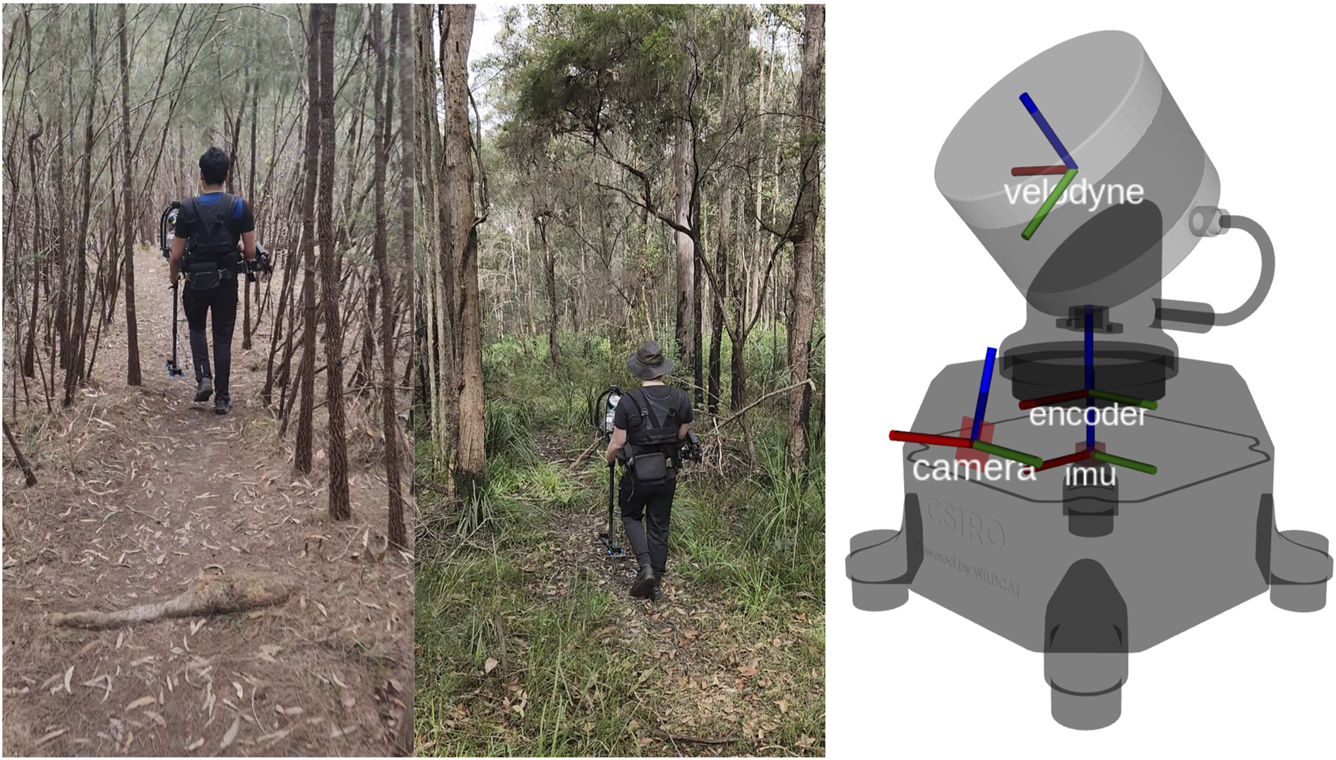
The dataset used for WildScenes benchmark is a multi-modal collection of traversals within Australian forests, allowing for a range of computer vision and robotic applications in natural environments. The WildScenes is divided into five sequences across two forest locations: Venman National Park and Karawatha Forest Park, Brisbane, Australia. These sequences are across different physical locations and also across different times. Please see Table 2 and Figure 2 for more details on the dataset traversals. The data was collected by walking through these locations with a portable, handheld sensor payload, as shown in Figure 3. For each traverse, we provide an accurate 6-DoF ground truth pose, manually annotated 2D semantic segmentation images, and generated 3D semantic segmentation point clouds. In total, WildScenes provides 9,306 images of 2016 × 1512 resolution and 12,148 associated point cloud submaps with greater than 70,000 annotated points per submap (on average). The number of points per submap can vary due to the spatial density of the environment, that is, due to the proportion of trees versus sky.

Figure 2.

The 3D semantic maps of the five traversals. The WildScenes contains repeat traversals of two natural environments, Venman (V-01, V-02, V-03) (left) and Karawatha (K-01, K-03) (right).

Figure 3.

Data collection campaign depicting the dense forest trails of Karawatha and Venman, respectively (left). The sensor payload comprises a spinning LiDAR sensor, encoder, IMU, GPS, and camera (right).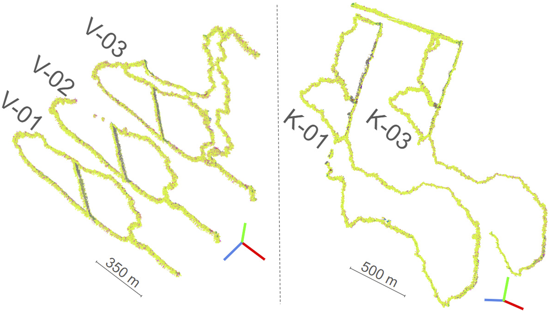

Our portable sensor setup includes a Velodyne Puck LiDAR sensor (consisting of 16 beams) attached to a brushless DC motor, rotating at a frequency of 0.5 Hz around the z-axis. This strategy is utilized to increase the vertical field-of-view and the 3D point density—given the Puck’s restricted vertical field-of-view (30 degrees), it is inclined at an angle of 45 degrees on the DC motor and rotated around an external axis. This setup enables LiDAR scans with a 120 degrees vertical Field-of-View (FoV), making it suitable for comprehensive top-to-bottom mapping of features such as trees. Additionally, it features a Microstrain 3DM-CV5-25 9-DoF IMU, an Ublox GPS antenna, and a Nvidia Jetson AGX Xavier. Pulse Per Second (PPS) is utilized to achieve sub-microsecond time synchronization accuracy among the sensors. The sensor payload is further equipped with four cameras for visual perception; however, we only use the front camera for annotation. We provide a complete summary of all sensor specifications in Table 3.

Table 3.

Sensor specifications used in WildScenes.

Sensor	Model	Rate (Hz)	Specifications
LiDAR^a	VLP-16	20	16 Channels
LiDAR^a	VLP-16	20	120 m Range
Camera x4	e-CAM130A CUXVR	15	94.9°H FOV
Camera x4	e-CAM130A CUXVR	15	71.2°V FOV
IMU	3DM-Cv5-25	100	9-DoF
GPS	Ublox-Neo-M8N	1

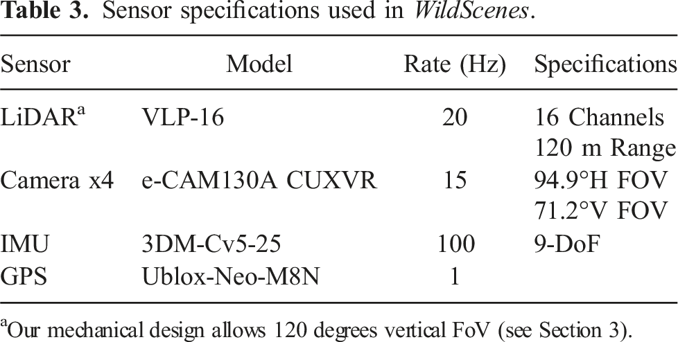
^aOur mechanical design allows 120 degrees vertical FoV (see Section 3).

To provide an accurate localization and mapping ground truth, we employ the LiDAR-inertial SLAM system Wildcat (Ramezani et al. (2022)) in which 6-DoF poses are optimized within a sliding window of LiDAR and inertial measurements captured in time. Our odometry system is devised to merge asynchronous IMU readings and LiDAR scans effectively through continuous-time trajectory representations (Bosse and Zlot (2009); Furgale et al. (2012); Droeschel and Behnke (2018); Park et al. (2021)). A primary benefit of continuous-time trajectory representation is to query corrected positions of LiDAR points at their timestamps, alleviating map distortion caused by the sensor’s motion. This is critical due to the extreme motions of the handheld mobile sensors.

To remove drift over time and generate a globally consistent map, we further incorporate GPS measurements into an offline bundle adjustment to optimize localization and mapping across the entire collection of IMU and LiDAR measurements, along with loop-closure constraints derived from a mechanism of loop-closure detection in revisit places. The bundle adjustment and the employed continuous-time trajectory representation allow the provision of a near-ground-truth trajectory and an undistorted map of the environment. This process allows us to release 3D point clouds that are globally aligned and consistent across an entire traverse, not just frame-to-frame. When creating the 3D point clouds, we apply a self-strike mask, a filter designed to exclude points that hit the person carrying the device. The radius set for the self-strike mask during our data post-processing is 2 m.

For the purpose of annotation, we sample a new image frame from the video stream for every five meters traveled or after every cumulative five degrees of rotation in the heading angle of the payload using the 6-DOF estimated global trajectory from SLAM. Since the sensor motion of the handheld sensor and the walking patterns of individuals can vary a lot, we employed this trajectory-centric sampling regime, as opposed to the commonly used equal temporal interval-based sampling, to ensure consistent sampling of all regions covered in the trajectory.

For each sample image, we generate a corresponding LiDAR submap (from the global map noted earlier) by accumulating points within a 45-m radius from the sensor frame and one second before and after the image timestamp. With precise sensor calibration and the retrieval of sensor 6-DOF pose from the SLAM-estimated trajectory, the projection of LiDAR submaps onto corresponding sample images is achievable. Additionally, we use camera intrinsic parameters to rectify sample images for the labeling process.

In summary, WildScenes is created using a pipeline of steps, from localization using LiDAR-inertial SLAM to human annotation of sampled images. After producing a trajectory-centric and globally aligned point cloud, we perform multi-frame label transfer from 2D into 3D to produce an accurate 3D semantic annotated map. Figure 4 summarizes this process.

Figure 4.

Overview of the LabelCloud pipeline for generaing a 3D semantic map. We use Wildcat SLAM to calculate the trajectory and global map. Then, after annotating the 2D images, we perform label transfer from 2D images across multiple frames into 3D, utilizing the 6-DOF trajectory, to produce our 3D semantic point cloud.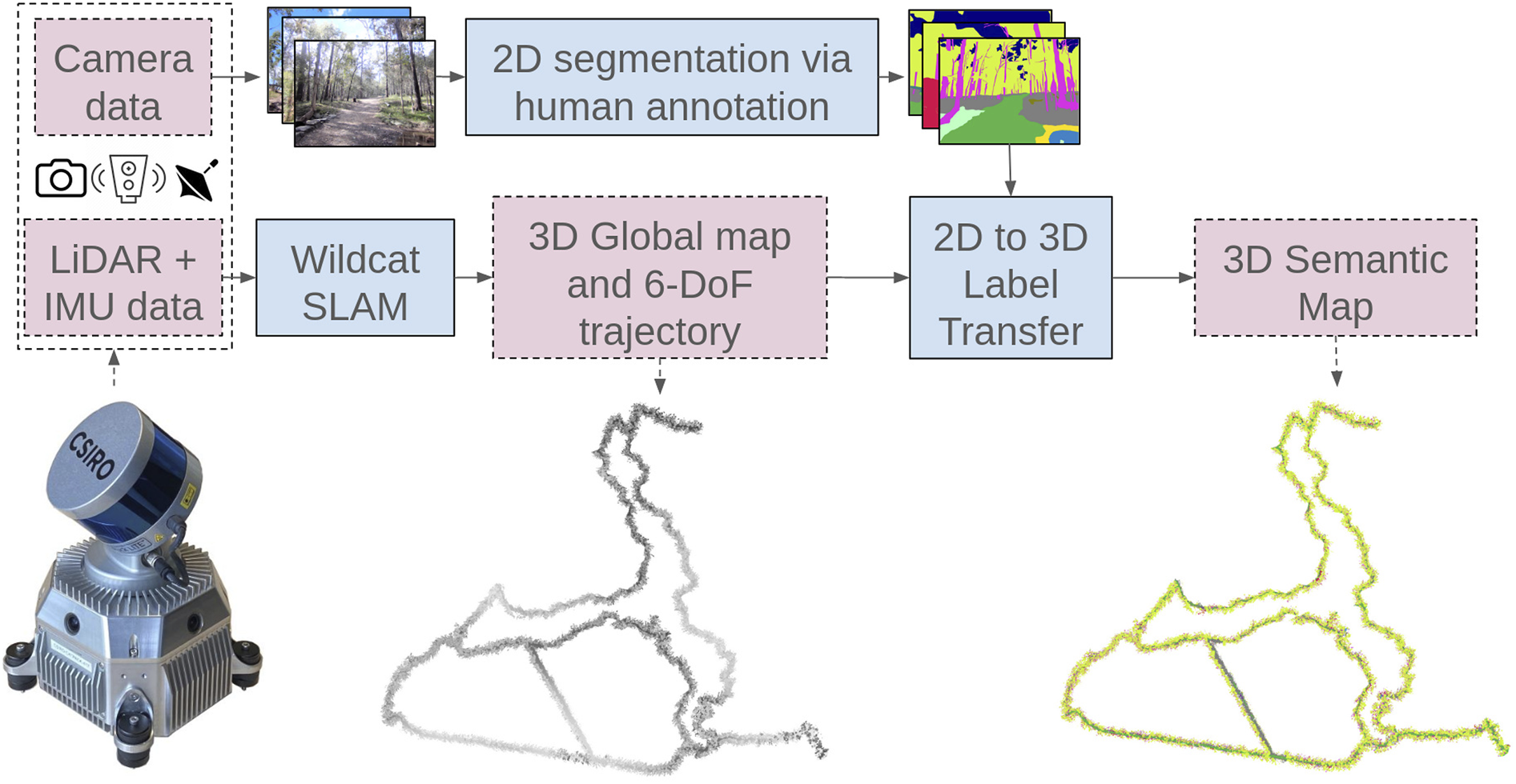

3.1. 2D semantic annotations

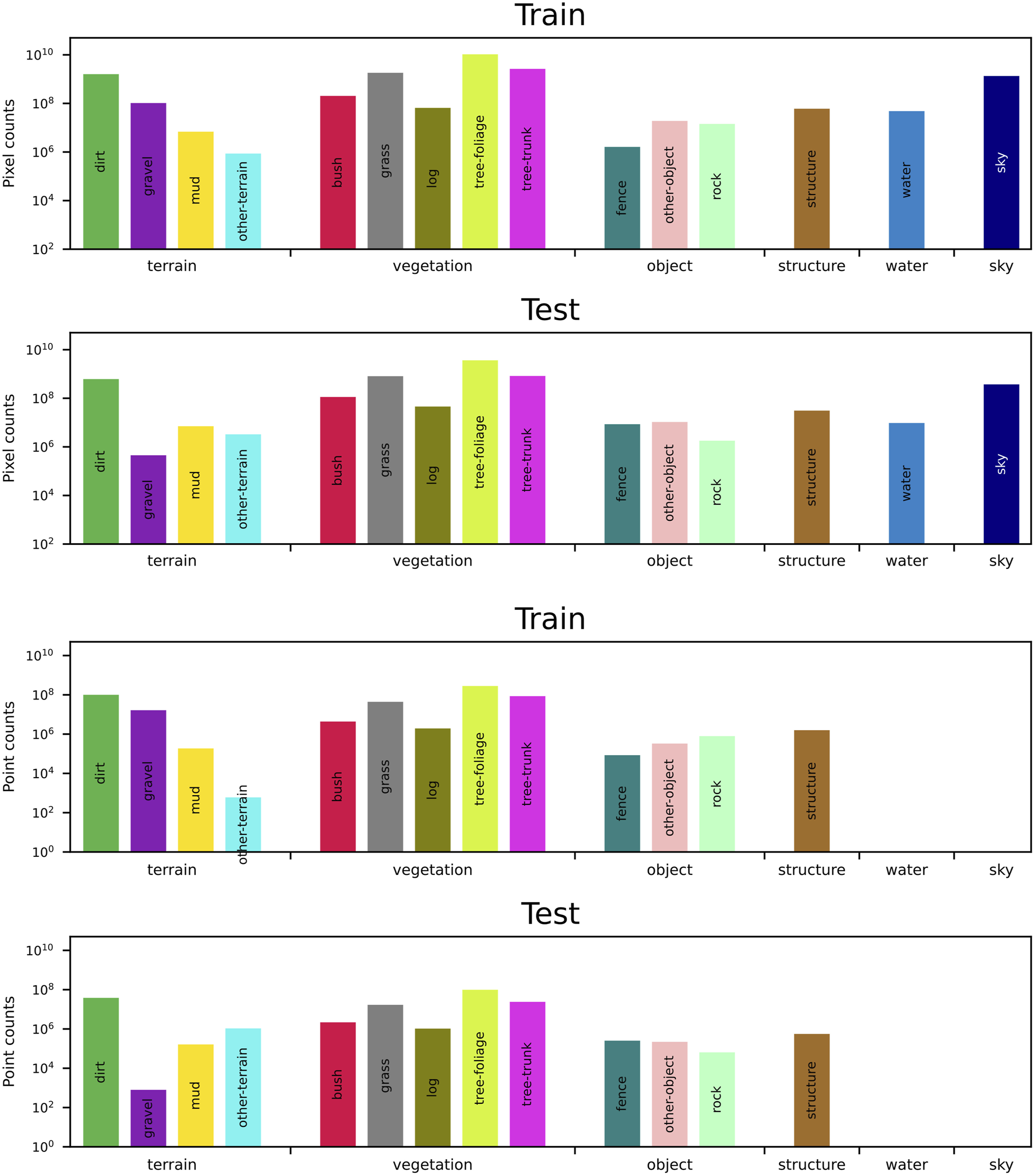
We provide manually annotated semantic segmentations for every sampled image in WildScenes, dividing the observed scene into a collection of different natural-scene classes. WildScenes comprises 15 different classes for the benchmark. Our class list is designed for natural environments and contains precise separation of vegetation types including, for example, tree-foliage (leaves) versus tree-trunk, and the distinction between different terrain features such as dirt and mud (as shown in Figure 5). Further details about our class list are provided in the WildScenes Supplementary Material section of this paper (Table 8).

Figure 5.

2D (top) and 3D (bottom) label counts of WildScenes. The dashed line in the 2D counts represents the threshold for exclusion of a class for evaluation.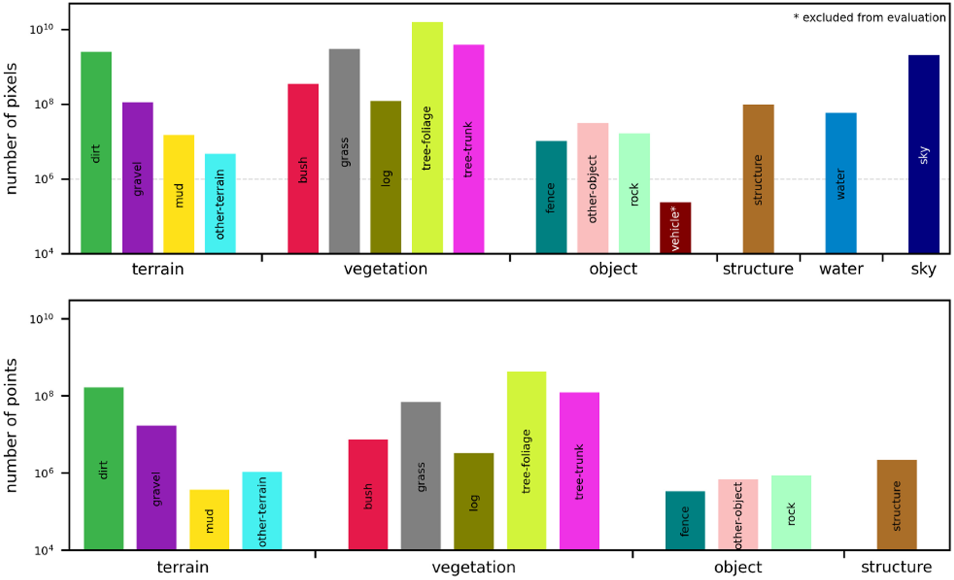

Several challenges arise when attempting to annotate unstructured, natural environments with such class specificity. In the wild, it can be hard to differentiate similar terrains or objects, such as dirt, mud, and gravel, depending on lighting conditions. Additionally, boundary ambiguity is a major issue due to the overlap of branches, leaves, bushes, etc. To mitigate these challenges, we follow a coarse-to-fine annotation approach to efficiently complete large-scale annotation while ensuring label quality and consistency with further refinements.

The first round of annotation produced coarse semantic labels by randomly distributing images between a group of experienced annotators. These annotations underwent multiple rounds of auditing to correct major errors and missing labels. All annotators used the same ontology for annotation, but due to the aforementioned ambiguity of classes and boundaries in natural environments, there were some inconsistencies in labels between different annotators.

To ensure consistent annotation, a final round of fine-grained auditing was done by a single trained annotator for approximately 250 h of annotation time. This audit focused on ensuring temporal consistency within sequences and enforcing class uniformity of features, as it was common for an ambiguous object to have differing class labels both intra-sequence and inter-sequence. This process significantly improved the quality and consistency of the coarse semantic annotations.

3.2. 3D annotations using LabelCloud

Compared to the manual annotation of 2D images, dense, cluttered, and unstructured natural environments make point-wise annotation of 3D point clouds very challenging. Forest environments have challenges, including occlusions and overlay between different semantic elements in the point cloud, the high spatial frequency of natural elements, and the inherent boundary ambiguities between different natural features such as dirt and mud. Therefore, the process of 3D annotating natural environments is more extensive in terms of both time and cost, resulting in practical infeasibility for large-scale datasets in dense forest environments.

To better facilitate large-scale 3D semantic annotation of point clouds, we propose a technique (named LabelCloud) for accurate and robust transfer of 2D semantic labels from multiple viewpoints onto a 3D point cloud. This process is depicted in Figure 4. LabelCloud is inspired by the 3D point colorization algorithm (Vechersky et al. (2018)), where each 3D point is assigned an RGB color according to their projections from image frames to point clouds. In this work, LabelCloud estimates the full distribution of label counts per 3D point. It also provides the mode over the distribution of 2D observations to find the most commonly observed labels.

A critical component of transferring data from a pixel in an image I_C(τ) acquired by camera C at time τ to a 3D point in a point cloud is ensuring the 3D point is visible in the image plane. To perform this task, we employ a multi-step process. The first step identifies the 3D points that are within a specific range of the camera C. This ensures that far-away observations of 3D structures where the image resolution is poor do not contribute to the final assessment of the 3D point. The next filter selects 3D points that project to valid pixel locations inside the image I_C(τ). The surface normal of a 3D point is then used to ensure that the 3D point is observable by the camera. The surface normal of a 3D point is calculated from the covariance matrix constructed from the neighboring 3D points. The eigenvector of the covariance matrix with the smallest eigenvalue is assumed to be the surface normal. The ambiguity in the direction of the surface normal is resolved by considering the position of the sensor payload at the time the 3D point was first observed.

The final step of identifying the visible 3D points addresses the problem of determining 3D structures that occlude other 3D structures. This is a challenging problem as 3D points have no volume, and it is improbable for two or more 3D points to lie on the same ray passing through the camera center. To address the problem, we employ the use of the generalized hidden point removal operator (Katz and Tal (2015)). The operator identifies visible points by performing a spherical reflection such that the order of points by distance is reversed, that is, 3D points that are closest to the camera center become the furthest and vice versa. The 3D points on the convex hull of the reflected point cloud are classified as visible. The function used to perform the spherical reflection governs how visibility is determined, and the inverse reflection of the edges connecting the 3D points on the convex hull represents the hallucinated 3D surface of the visible points. In this work, we use the exponential inversion kernel to perform the reflection due to its scale-invariant properties (Vechersky et al. (2018)).

Having identified the 3D points that are visible in the image I_C(τ), it is now straightforward to augment information about each visible 3D point with its corresponding image pixel. We begin by projecting the set of visible 3D points onto the image, then returning the observed label at the corresponding pixel location. We then repeat this process for all images, and if a given 3D point is visible in multiple images, then we aggregate all 2D labels that we acquire from projection. To find the final label per point, we find the most commonly observed label, that is, the mode over the distribution of 2D observations. A visualization of this process is provided in Figure 6. Note that if a 3D point is not visible in any image, we drop this point from our labeled point cloud output.

Figure 6.

An illustration of how 3D semantic labels are generated from the 2D labeled images. We first compute the set of images which observe a single 3D point (shown as viewpoint 1-n). A histogram of labels for the 3D point is then calculated by projecting the 3D point on to each image and recording the associated 2D label. The 2D label with the highest number of observations is then transferred to the 3D point. This example shows the label transfer for a point on a tree-trunk. We see two votes for the label “tree-trunk” and one vote for the label “tree-foliage.”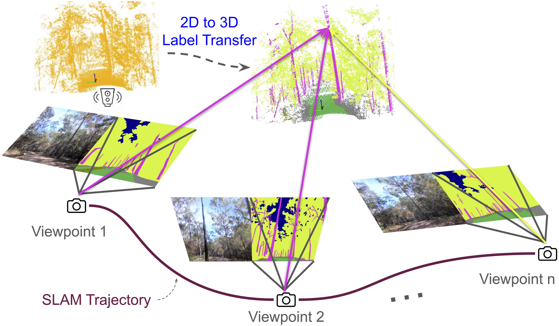

Furthermore, we also record the full distribution of 2D observations for each 3D point, providing a histogram of label observations per point. This provides several benefits: firstly, it provides an opportunity to measure the consistency of the 2D semantic labels for a specific 3D point. Secondly, the most probable semantic label for each 3D point can still be used to train 3D semantic segmentation algorithms. Finally, by providing the full distribution of label observations, we hope to provide an avenue for future researchers to use this data to explore novel research areas such as uncertainty-aware (Sirohi et al. (2023); Cortinhal et al. (2020)) or multi-label semantic segmentation (Zhu et al. (2019)). Hereafter, we refer to this multi-view aggregation of observations as our label histogram.

Therefore, for each 3D point, we generate a label histogram Pⁱ for the i^th point, where $|P^{i}| = C$ and C is the number of classes in WildScenes. Such a distribution could have a myriad of future applications, such as label distribution learning or uncertainty-aware perception. We provide a quantitative analysis of this label ambiguity in our results and discussion section.

3.3. Split generation

As WildScenes was recorded from sequential traversals of natural environments, there exists a risk of geographical proximity between the train/test/validation sets. Additionally, it is important to have train, validation, and test sets with a uniform class distribution.

To address this, we developed a split generation procedure that adds buffer regions between sets while also ensuring a good class distribution. As our 3D submaps have a radius of 45 m, we added buffer regions such that there is a minimum distance of 45 m between samples from different sets. The buffer regions are designed to ensure no visual overlap between train/val/test splits (2D and 3D).

We used a modified version of the split generation procedure proposed by Almin et al. (2023b) to generate an optimized split that satisfied our requirements. In summary, the algorithm generates a large number of candidate splits by randomly assigning chunks of the trajectory into candidate sets and then selects the best split based on a number of metrics and constraints. As WildScenes contains a number of sequences across different times, samples were grouped based on their 2D (x,y) coordinates with k-means clustering for K = 50. This was performed to bias the generation of candidate splits towards less interleaving. The parameter k represents a tradeoff where smaller K allows a larger space of candidate splits but biases the candidates towards highly interleaved splits with large numbers of images lost to the buffer.

Subsequently, 1000 candidate splits were generated with random initialization, each satisfying the constraint that all (train/val/test) sets had at least one instance of each class. We used the Label Distribution (m_LD), the Inverse Frequency Weighted Label Distribution (m_IF), and the Label KL Divergence (m_KL) to calculate a fitness score for each of these candidates. In summary, these metrics estimate the divergence between the class distribution in a subset of a given split compared to the class distribution of the full dataset. Ideally, the distribution of class counts in a given split should match the class distribution of the full dataset.

Unlike the work in Almin et al. (2023b), because of the need to include buffer regions, we added the Silhouette Coefficient (m_SC) (Rousseeuw (1987)) as an additional metric. m_SC calculates how tightly grouped each of the sets is in metric space with respect to the other sets. m_SC is defined as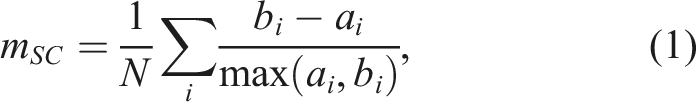

m_{S C} = \frac{1}{N} \sum_{i} \frac{b_{i} - a_{i}}{\max (a_{i}, b_{i})},

(1)

where a_i is the mean intra-split distance and b_i is the mean nearest-split distance for sample i, for all samples N in each split. A high m_SC value means the split contains samples from a similar metric location, while a low m_SC value means there is a large amount of interleaving between sets.

The final split quality was calculated using a normalized and weighted combination of the aforementioned metrics: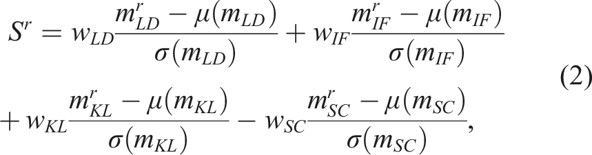

\begin{align} S^{r} = w_{L D} \frac{m_{L D}^{r} - μ (m_{L D})}{σ (m_{L D})} + w_{I F} \frac{m_{I F}^{r} - μ (m_{I F})}{σ (m_{I F})} \\ + w_{K L} \frac{m_{K L}^{r} - μ (m_{K L})}{σ (m_{K L})} - w_{S C} \frac{m_{S C}^{r} - μ (m_{S C})}{σ (m_{S C})}, \end{align}

(2)

where r is the index of the random split in R and |R| = 1000. The optimal split was found by finding the random split with the minimum score S^r, using the 2D labels as the input to the algorithm. We set w_LD = 1, w_IF = 1, w_KL = 1 and w_SC = 2. We prioritize the Silhouette Coefficient metric because we found that excessive generation of buffer regions significantly reduced the size of our train/val/test sets.

We also show a metric map showing the distribution of our splits and their associated buffer regions between them (Figure 7). Finally, in Figure 8, we show the label counts for each class in our optimized split.

Figure 7.

Metric maps of the WildScenes benchmark dataset showing the geographical distribution of train/val/test sets and buffer regions.

Figure 8.

Label distributions in both 2D (top) and 3D (bottom) for our optimized train and test sets (log scale).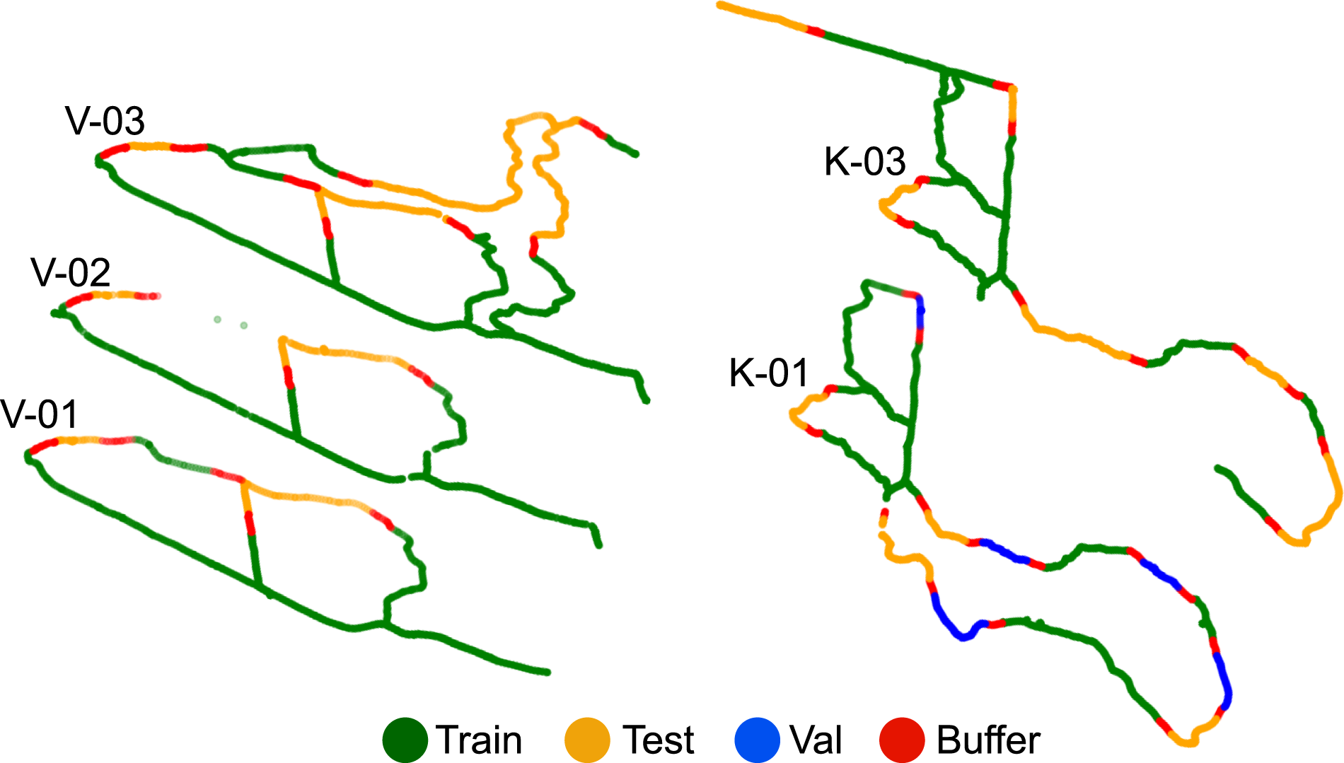

4. Benchmark experiments

4.1. Benchmark split

Using our split generation procedure detailed earlier, we split our dataset into train/val/test splits with 6051/283/2133 images and 7517/356/2705 point clouds, respectively (or an objective split ratio of 70%, 5%, 25%). Note that the total number of images and point clouds in these splits are less than the total contained in WildScenes, since some images and point clouds are allocated to the buffer regions.

4.2. 2D benchmark experiment

We benchmark four different approaches for 2D semantic segmentation. We use DeepLabv3 (Chen et al. (2019)) with a Resnet-50 backbone, Mask2Former (Cheng et al. (2022)) with a Resnet-50 backbone, Mask2Former with a Swin-L backbone, Segformer (Xie et al. (2021)) MiT-B5 variant, and UPerNet (Xiao et al. (2018)) with a ConvNeXt-L backbone as our baseline methods to benchmark on our proposed dataset. These methods were chosen with different rationales. DeepLabv3 was chosen as a traditional architecture that has been commonly used in recent literature as a benchmark (Strudel et al. (2021); Li et al. (2022); Cheng et al. (2021)). As a second technique, we selected Mask2Former to provide a state-of-the-art architecture (on ADE20k (Zhou et al. (2017)), excluding methods with more than one billion parameters) for semantic segmentation. We selected a transformer backbone (Swin-L, pre-trained on ImageNet-22k (Deng et al. (2009))) and a convolutional backbone (Resnet-50) to investigate whether large pre-trained transformer models offer any benefits to our dataset. For our third baseline method, we selected the largest model of SegFormer (SegFormer-B5), to provide an alternate transformer segmentation network. Finally, to understand the differences between transformer and convolutional architectures on our dataset, we selected a convolutional-only method with a parameter count comparable to a large transformer architecture. Therefore, we selected Conv-NeXT-L (197 million parameters) with an UPerNet head as our fourth benchmark technique.

4.2.1. Training procedures

We use the mmsegmentation codebase¹ for running all our 2D semantic segmentation benchmarks. For all baselines, we train for 80k iterations, with a batch size of 40, using two Nvidia H100 GPUs. We consistently use a crop size of (512, 512). We employ the augmentations: RandomResize, RandomCrop, and RandomFlip. We employ the learning rates, optimizer, and scheduling as per the defaults for each baseline method, only adjusting the scheduler to suit our batch size. We initialize the backbones of all 2D networks with pre-trained weights from either ImageNet-1k (Deeplabv3, Mask2Former Resnet, SegFormer) or ImageNet-22k (Mask2Former Swin, UPerNet ConvNeXt).

4.3. 3D benchmark experiment

We benchmark four different approaches for 3D semantic segmentation. We utilize SPVCNN (Tang et al. (2020)), Cylinder3D (Zhu et al. (2021)), MinkUNet (Choy et al. (2019)) and SphereFormer (Lai et al. (2023)). We selected these methods due to their high performance on the common 3D semantic segmentation benchmark SemanticKITTI (Behley et al. (2019)) and the availability of an open-source implementation. Because LiDAR returns are non-existent or inaccurate on the “sky” and “water” classes, respectively, we exclude these classes from evaluation for our 3D benchmarking. We also exclude the class “other-terrain” due to an inadequate number of points in the train set, leading to a total of 12 classes for the 3D benchmark.

4.3.1. Training procedures

For all 3D benchmarking, we use the mmdetection3d codebase² and the SphereFormer codebase.³ For all baselines, we train for 50 epochs with a batch size of 20 on one or two NVIDIA H100 GPUs. We employ the augmentations: RandomRotation, RandomScale, RandomTranslate, RandomFlip. We employ each method’s default learning rate, optimizer, and scheduling and all 3D networks are initialized with random weights.

4.4. Evaluation criteria

For evaluating the performance of a semantic segmentation method with respect to the ground truth label annotations, we use the standard Mean Intersection over Union (mIoU) metric for a set of 15 classes (2D) and 12 classes (3D).

5. Results and discussion

5.1. 2D semantic segmentation

In Table 4, we display the results of our benchmark experiments on WildScenes. Considering the task of 2D semantic segmentation, we observe that WildScenes provides a challenging benchmark for existing techniques with a peak mIoU of 47.85 from Mask2Former with a Swin-L backbone, closely followed by 47.3 from UPerNet with a ConvNeXt-L backbone. Considering that M2F achieves 56.1 (Cheng et al. (2022)) and ConvNeXt-L achieves 53.7 (Liu et al. (2022)) on ADE20k-val, it is clear that WildScenes dataset has challenging properties for semantic segmentation.

Table 4.

Benchmark semantic segmentation on the WildScenes Test Set. The top half of the table shows the results for 2D segmentation and the bottom half for 3D segmentation.

	Method	mIoU	bush	dirt	fence	grass	gravel	log	mud	other-object	other-terrain	rock	sky	structure	tree-foliage	tree-trunk	water
2D	DeepLabv3 (Resnet-50)	43.37	14.79	73.23	0.29	63.67	18.72	34.12	18.43	64.83	0	27.88	80.53	49.25	85.89	62.03	56.94
	Mask2Former (Resnet-50)	43.71	25.18	74.25	0.40	62.20	5.72	36.42	20.52	53.24	0	33.50	80.45	56.89	86.07	62.12	58.70
	Mask2Former (Swin-L)	47.85	23.18	74.67	0.51	63.01	7.36	46.85	21.40	60.59	0	60.05	80.57	64.22	86.15	63.28	65.97
	Segformer (MiT-B5)	40.83	13.16	73.32	0.24	59.97	7.11	29.64	2.88	54.67	0.20	38.30	79.35	53.01	84.50	61.42	54.70
	UPerNet (ConvNeXt-L)	47.30	13.78	75.15	0.35	63.79	15.61	39.97	16.85	69.14	4.96	55.68	80.48	60.97	85.98	62.90	63.95
3D	SPVCNN	36.78	18.88	83.55	10.84	70.27	0	18.42	0.19	29.45	—	7.68	—	54.32	89.73	58.02	—
	Cylinder3D	40.07	30.61	82.92	4.81	69.80	0	28.12	6.60	35.08	—	19.39	—	55.16	89.84	58.54	—
	MinkUNet	36.53	18.99	83.89	9.88	70.20	0	22.81	0.89	27.79	—	1.04	—	55.40	89.68	57.74	—
	SphereFormer	33.97	12.28	78.00	7.73	49.65	0	27.54	0.69	28.15	—	17.59	—	51.88	85.23	48.90	—

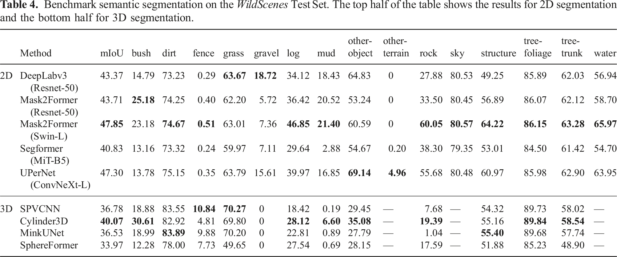
While the mean IoU metric is important for a general performance measure, as a result of the long-tailed distribution of class frequencies in natural environments (refer to Figure 5), it is skewed by the presence of rarely occurring classes with a poor IoU score. Our four least common classes are other-terrain, mud, fence, and rock. Our four lowest performing classes using Mask2Former+Swin-L are other-terrain, fence, mud and gravel, with IoU scores of 0, 0.51, 21.4 and 7.36, respectively. Infrequent classes have low IoU at test time, which is a result of the lack of training samples from which the network can learn. This opens up an interesting direction for future research considering how to design or pre-train semantic segmentation networks to handle uncommon classes.

However, the number of class labels represents only part of the overall context. For example, even though gravel only achieves an IoU of 7.36, it is relatively commonly occurring with 10⁸ annotated pixels across the dataset. Furthermore, tree-trunk is very common ( $> 1 0^{9}$ annotated pixels) but only achieves an IoU of 63.28. We hypothesize that the unstructured and ambiguous properties of natural environments are additional contributing factors to the performance of semantic segmentation on specific classes.

Another observation is the low performance of the fence class. We note that the fence class is adequately present in both training and test sets; however, as a coincidental result of our split optimization, one design of fence (a fence with a single horizontal railing) appears in the train set while the fence in the test set has three horizontal railings. Therefore, we suspect that none of the networks can successfully generalize between different fence designs based on the existing training data.

Comparing the performance of different networks for certain classes (e.g., dirt, tree-foliage, sky, tree-trunk, grass), the IoU score is almost the same for any network. While for other classes (e.g., bush, gravel, rock, log), the IoU score varies considerably between different networks. The key difference is that the aforementioned stable classes are also the top-5 most common classes in terms of pixel counts (see Figure 5). We hypothesize that differing network architectures and pre-trained configurations have a larger influence on classes with a reduced number of training samples, resulting in the observed differences in IoU between different networks. Another observation is that Segformer is the lowest performing method (by mIoU score). One difference is that Segformer is pre-trained on ImageNet-1K (Xie et al. (2021)), while ConvNeXt-L and Swin-L are pre-trained on the larger ImageNet-22K, and we hypothesize that the reduced pre-training means that the network requires more training samples for the less common classes.

5.2. 3D semantic segmentation

On the bottom half of Table 4, we provide the benchmark performance of 3D point cloud segmentation methods. We observe that 3D semantic segmentation is a challenging task on WildScenes, with the highest mIoU of 40.07 achieved by Cylinder3D (Zhu et al. (2021)). Overall, we observe that all techniques have a relatively similar mIoU; while it is expected that SPVCNN (Tang et al. (2020)) will perform similarly to Cylinder3D (since they have a similar mIoU on SemanticKITTI), there are little variations in mIoU between techniques. We hypothesize that the unstructured properties of natural environments limit the ability of these networks to perform semantic segmentation, with some classes being much easier to classify than others.

We observe a considerable variation in IoU between different classes in 3D. Commonly occurring classes such as dirt and tree-foliage achieve a consistently high IoU score across all four benchmark methods. In fact, we find that point cloud segmentation networks are more accurate at identifying dirt than 2D segmentation networks. While grass and tree trunk are also common classes (approximately 10⁷ and 10⁸ points, respectively), we observe a notable drop in IoU to approximately 70% and 60%, respectively. And yet, structure has an IoU of approximately 55% even though it is significantly less common in terms of class label counts—approximately 10⁶ 3D points. We attribute this to the distinctness of classes. As the only information received by the network is the 3D coordinates of points across 3D space, classes that have distinctive shapes and surfaces in 3D are more likely to be easy to classify (e.g., structures, fences).

In another example, the classes bush and log both experience low IoU scores of around 20% and yet are more commonly occurring than structure. We hypothesize that it is likely difficult to distinguish between bush and tree-foliage, and between log and tree-trunk, as these classes are naturally ambiguous with each other, especially in 3D where there is no color information available. We suggest that an interesting avenue of future work using WildScenes would be to use geometric projection to supplement a point cloud with color information from images, which may aid in perception in these types of unstructured natural environments.

Finally, as in 2D, we observe that tail classes that rarely occur are difficult to learn from with existing training paradigms. In 3D, our five least common classes are mud, fence, other-object, other-terrain and rock. We find that all these classes have low IoU scores, although fence achieves a surprisingly high IoU (relative to its counterpart in 2D) of up to 10.84% with SPVCNN (Tang et al. (2020)), even though it is a rare class with just 10⁵ 3D points. Again, as was the case with structure, fence is an object type with a distinctive and structured shape in 3D, which likely provides a bias toward the ability of a network to learn to classify this class. Finally, we observe that gravel is unable to be learned by any network, even though there are 10⁷ points in the dataset. We hypothesize that gravel, alongside mud, is difficult to identify in 3D due to sharing a very similar shape and environmental context to the extremely common class dirt.

5.3. Impact of temporal and environmental domain shifts

WildScenes is comprised of both repeat traverses of the same natural environment across 6 months and traversals across spatially separate environments. This allows us to quantitatively evaluate the performance of our trained semantic segmentation models in the presence of a domain shift, that is, a shift in the data distribution between the training and testing sets as a result of either a change in location or due to changes in the natural environment over time.

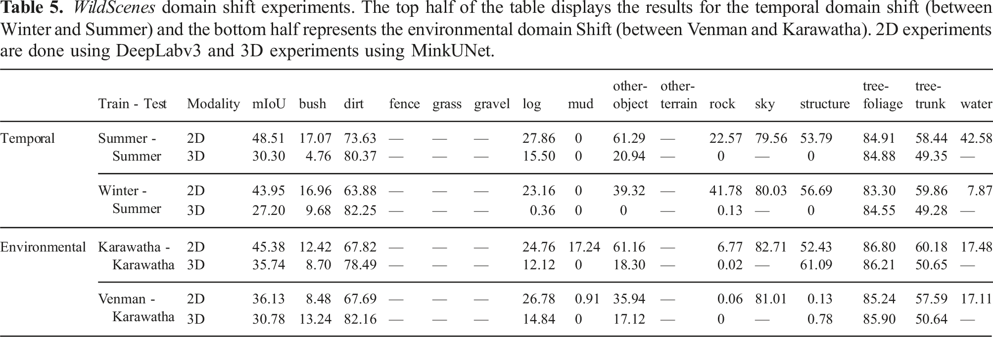
For this experiment, we generated four new train/val/test splits, which are subsets of the existing optimized split. Our splits are detailed below (the validation set always stays the same):

• Summer to Summer: train and test on sequences from December (Summer season in Australia) (V-03 and K-03). Train and test sets maintain geographic separation. Train: 3742 images, Test: 1499 images.

• Winter to Summer: train on June (Winter season in Australia) (V-01, V-02 and K-01), test on December (V-03 and K-03). Train: 2309 images, Test: 1499 images.

• Karawatha to Karawatha: train on the training regions from K-01 and K-03, and test on the test regions from K-01 and K-03. Train: 3809 images, Test: 1247 images.

• Venman to Karawatha: train on the training regions from V-01, V-02 and V-03, and test on the test regions from K-01 and K-03. Train: 2242 images, Test: 1247 images.

We provide benchmarks for training and testing on these sub-splits in Table 5 for both 2D (using Deeplabv3) and 3D (using MinkUNet), and visualize the impact of the temporal and environmental domain shifts on test-time performance in Figure 9. Note that we exclude the classes gravel and other-terrain from evaluation on these sub-splits, due to very low class counts in either the train or test set.

Table 5.

WildScenes domain shift experiments. The top half of the table displays the results for the temporal domain shift (between Winter and Summer) and the bottom half represents the environmental domain Shift (between Venman and Karawatha). 2D experiments are done using DeepLabv3 and 3D experiments using MinkUNet.

	Train - Test	Modality	mIoU	bush	dirt	fence	grass	gravel	log	mud	other-object	other-terrain	rock	sky	structure	tree-foliage	tree-trunk	water
Temporal	Summer - Summer	2D	48.51	17.07	73.63	—	—	—	27.86	0	61.29	—	22.57	79.56	53.79	84.91	58.44	42.58
	Summer - Summer	3D	30.30	4.76	80.37	—	—	—	15.50	0	20.94	—	0	—	0	84.88	49.35	—
	Winter - Summer	2D	43.95	16.96	63.88	—	—	—	23.16	0	39.32	—	41.78	80.03	56.69	83.30	59.86	7.87
	Winter - Summer		3D	27.20	9.68	82.25	—	—	—	0.36	0	0	—	0.13	—	0	84.55	49.28	—
Environmental	Karawatha - Karawatha	2D	45.38	12.42	67.82	—	—	—	24.76	17.24	61.16	—	6.77	82.71	52.43	86.80	60.18	17.48
	Karawatha - Karawatha	3D	35.74	8.70	78.49	—	—	—	12.12	0	18.30	—	0.02	—	61.09	86.21	50.65	—
	Venman - Karawatha	2D	36.13	8.48	67.69	—	—	—	26.78	0.91	35.94	—	0.06	81.01	0.13	85.24	57.59	17.11
	Venman - Karawatha		3D	30.78	13.24	82.16	—	—	—	14.84	0	17.12	—	0	—	0.78	85.90	50.64	—

Figure 9.

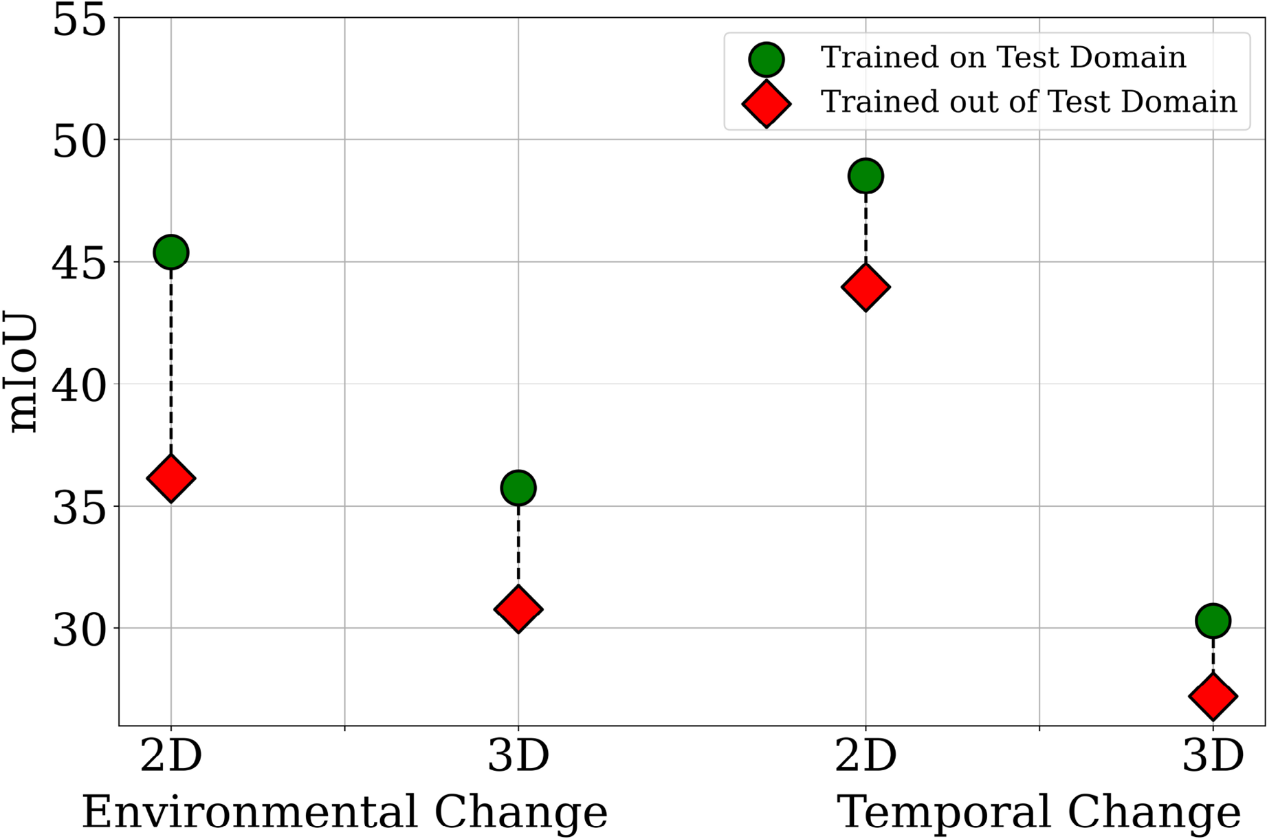
Visualization of the performance drop due to environmental or temporal domain shifts between the training and testing sets. “Environmental Change” estimates the domain gap between Venman and Karawatha, and “Temporal Change” estimates the domain gap between Winter and Summer. “Trained on Test Domain” refers to experimental setups where the training and testing splits are in-domain (e.g., Summer to Summer), whereas “Trained out of Test Domain” refers to setups where there is either an environmental or temporal domain shift between the training and testing splits (e.g., Winter to Summer).

5.3.1. Temporal domain shift

In 2D, we observe that semantic segmentation performs better when no temporal domain shift occurs with respect to the training data, as expected. In natural environments, it is expected that vegetation classes, especially tree-foliage, grass, and bush, will change more rapidly over time than features such as rock, structures, objects, and dirt. Furthermore, vegetation can also change color due to seasonal changes. For example, it can be observed that the IoU for grass is higher in Summer to Summer (60.4) than in Winter to Summer (54.54). In 3D, a similar but smaller trend exists. For example, the grass class IoU increases from 45.77 to 47.16 when the training season is the same as the test season. This is not surprising—grass is likely to be the type of vegetation that grows the fastest and is most affected by seasonal differences. However, the inverse trend exists for the bush class with a drop in IoU of 4.92; although, as bush is a rare class there may be insufficient training data (in these inter-sequence splits) for stable training of this class.

5.3.2. Environmental domain shift

In addition to the above results, we observe that the mIoU drops considerably for both 2D and 3D modalities when there is an environmental domain shift between the training and testing data. Some classes are highly impacted by the environment used for training. For example, structures are only able to be detected in the Karawatha test set when Karawatha is also used for training—this indicates that the types of structures in Venman are very different in their style/design and are unable to generalize to structures in Karawatha (in both 2D and 3D).

A number of classes also appear to be invariant to the physical location of the training set. We observe that dirt, grass, log, sky, tree-foliage, tree-trunk and water are almost unchanged in their IoU when the training environment changes from Karawatha to Venman. This is an expected result since these classes comprise features that are commonly found in natural environments. However, we note that since both environments are located in Australia, we would expect a greater impact on IoU if a training or testing set from a natural environment in another country was used. This would be an interesting avenue for future work.

5.4. Label histograms

As discussed earlier, our 3D annotation procedure allows us to provide label distributions for every 3D point. We provide a histogram of the number of times a given class was assigned to that point from all 2D semantic labels (observations from human annotators across multiple frames) of that point. We propose that natural environments are naturally ambiguous and do not easily conform to rigid semantic label assignments. For example, the difference between dirt and mud is small since mud is simply wet dirt. Or, a small tree could be confused with a bush/shrub. In this section, we analyze which classes are co-occurring in the label histograms to understand which pairs of classes are naturally ambiguous with each other.

To measure the semantic ambiguity—the inconsistency in annotation due to the natural ambiguity of natural environments—we calculate co-occurrences between classes in the histograms. We calculate the co-occurrences for each 3D point, then aggregate across all 3D points in our dataset. Our results are shown in Figure 10, representing the same data in both matrix form and using a chord diagram. In the matrix, a larger value of a class diagonal denotes a less ambiguous class, that is, a class where all 2D observations had the same label. In the chord diagram, the arrows signify which pairs of classes are co-occurring with each other.

Figure 10.

Utilizing the histograms of labels produced by label transfer, we can calculate the co-occurrences of different classes, that is, for a given 3D point, what labels were assigned from all of its viewpoints. Left: we plot the co-occurrences in matrix form, with all rows normalized to sum to one. Right: we represent co-occurrences via a chord diagram. A larger outer segment denotes a class with greater co-occurrences with other classes, and the directions of the curves denote which pairs of classes are co-occurring.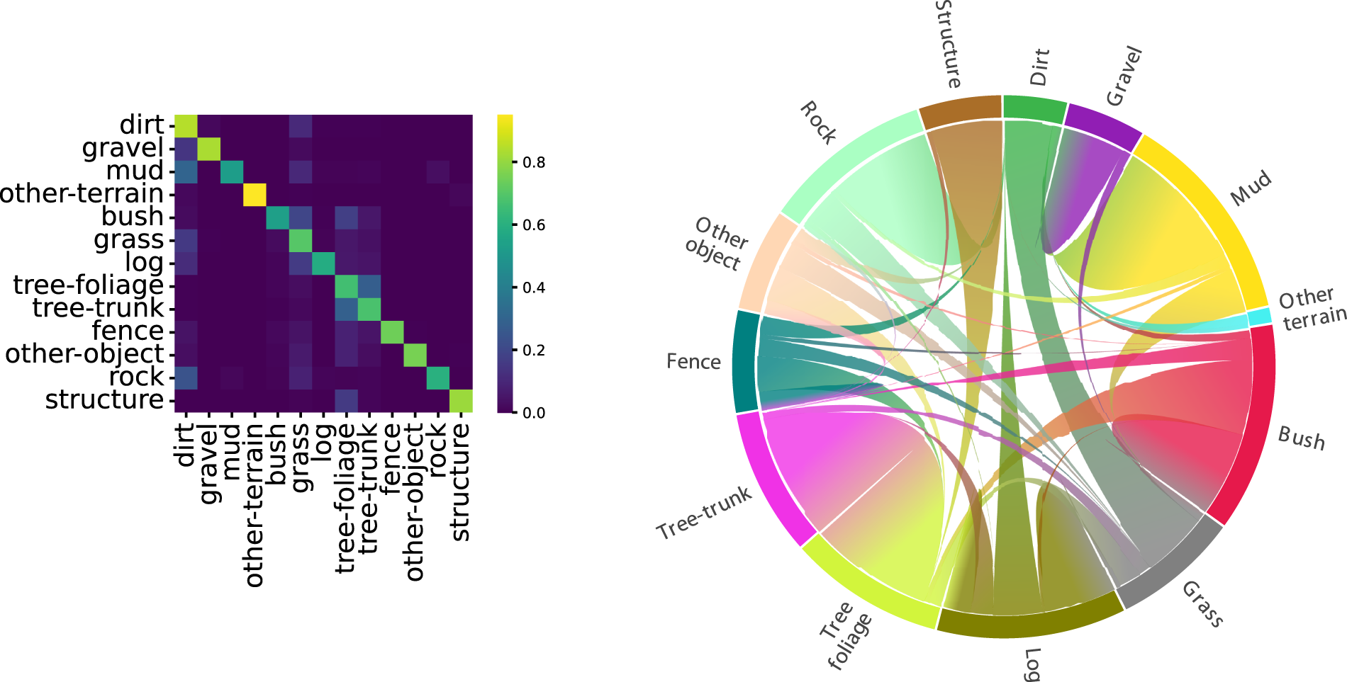

From these plots, we can make the following conclusions. First, a large proportion of mud points have also been labeled as dirt, however, conversely, only a small fraction of dirt points have been given mud labels in 2D (noting that there are approximately 10⁵ mud points vs 10⁸ dirt points). Tree-trunk and tree-foliage are also co-occurring, however, this is not unexpected—WildScenes contains sections of dense forest trails where a fine-grained segmentation between tree leaves and branches becomes ill-defined, especially from a distance. However, overall, the mean value of the diagonal of the co-occurrence matrix is 0.71. Therefore, the total disparity in 2D observations is still small, which is a result of our fine-grained annotation auditing procedure. We provide these label histograms with our benchmark dataset release, which could be used in future work such as uncertainty-aware semantic segmentation in natural environments.

6. Conclusion

In this paper, we have introduced WildScenes, a new benchmark dataset for 2D and 3D semantic segmentation in natural environments. WildScenes comprises traverses across multiple different natural forest environments over an extended time period and provides high-resolution 2D images and dense 3D LiDAR point clouds with full point/pixel level annotation. Additionally, we use LiDAR SLAM to provide accurate 6-DoF pose information for all camera and LiDAR submap timestamps. WildScenes comprises 9,306 annotated images and 12,148 annotated 3D point cloud submaps, across 21 km of walking through densely vegetated natural environments. The annotation divides the natural environment into 15 classes, classifying both different vegetation types (e.g., bushes/shrubs vs trees) and different terrain types (e.g., dirt vs gravel), along with other features including fences and structures.

We provide an initial benchmark using state-of-the-art 2D and 3D segmentation methods on WildScenes, to demonstrate the additional challenges present in unstructured natural environments. We demonstrate that WildScenes poses challenges for existing segmentation methods in both 2D and 3D, as a result of the inherent semantic ambiguity and long-tail distribution of class occurrences in natural environments. In addition, by providing accurate 6-DoF pose information for both the image and LiDAR modalities we open up the opportunity for future researchers to investigate multi-modal segmentation approaches which can leverage the advantages of both modalities—the rich color and textural information from RGB images as well as the 3D geometric structure provided by the LiDAR point cloud.

We expect that WildScenes will aid in the development of future perception systems for autonomy for applications such as search and rescue, conservation, and agricultural automation, for which existing urban perception datasets are ill-suited. Future work includes developing novel methods for semantic segmentation in both 2D and 3D, designed specifically for segmentation in natural environments. Additional future work also includes expanding this dataset to include instance annotations. For example, the inclusion of instance annotations for different trees would provide value in training networks for tree detection and classification. Combining all of these aspects, we believe WildScenes provides a valuable resource for the future development of semantic segmentation techniques for robust autonomous perception in natural environments.

Footnotes

Acknowledgments

The authors gratefully acknowledge funding of the project by the CSIRO’s Machine Learning and Artificial Intelligence (MLAI) FSP and continued support from of the CSIRO’s Data61 Embodied AI Cluster. This work would not be possible without support from members of the CSIRO Robotics including Brett Wood, Dennis Frousheger, Nick Hudson, Paulo Borges, Gavin Catt, Fred Pauling, Dave Haddon, and Stano Funiak.

Declaration of conflicting interests

The author(s) declared no potential conflicts of interest with respect to the research, authorship, and/or publication of this article.

Funding

The author(s) received no financial support for the research, authorship, and/or publication of this article.

ORCID iDs

Kavisha Vidanapathirana

Stephen Hausler

Mark Cox

Ethan Griffiths

Peyman Moghadam

Notes

Appendix

References

Almin

Lemarié

Duong

, et al. (2023a) Navya3dseg-navya 3d semantic segmentation dataset design & split generation for autonomous vehicles. IEEE Robotics Automation Letters 8: 5584–5591.

Almin

Leo

Duong

, et al. (2023b) Navya3dseg – navya 3d semantic segmentation dataset and split generation for autonomous vehicles. DOI:10.48550/arXiv.2302.08292.

Baghbaderani

Wang

, et al. (2024) Temporally-consistent video semantic segmentation with bidirectional occlusion-guided feature propagation. In: Proceedings of the IEEE/CVF Winter Conference on Applications of Computer Vision, Waikoloa, HI, 03–08 January 2024, pp. 685–695.

Behley

Garbade

Milioto

, et al. (2019) Semantickitti: a dataset for semantic scene understanding of lidar sequences. In: Proceedings of the IEEE/CVF International Conference on Computer Vision, October 27th to November 2nd 2019, Seoul, South Korea, pp. 9297–9307.

Behley

Garbade

Milioto

, et al. (2021) Towards 3d lidar-based semantic scene understanding of 3d point cloud sequences: the semantickitti dataset. The International Journal of Robotics Research 40(8–9): 959–967.

Borges

Peynot

Liang

, et al. (2022) A survey on terrain traversability analysis for autonomous ground vehicles: methods, sensors, and challenges. Field Robotics 2(1): 1567–1627.

Bosse

Zlot

(2009) Continuous 3D scan-matching with a spinning 2D laser. In: 2009 IEEE international conference on robotics and automation,Kobe, Japan, 12–17 May 2009, pp. 4312–4319. IEEE.

Burnett

Yoon

, et al. (2023) Boreas: a multi-season autonomous driving dataset. The International Journal of Robotics Research 42(1–2): 33–42.

Chen

Papandreou

Schroff

, et al. (2019) Rethinking atrous convolution for semantic image segmentation. arxiv 2017. arXiv preprint arXiv:1706.05587 2.

10.

Cheng

Schwing

Kirillov

(2021) Per-pixel classification is not all you need for semantic segmentation. Advances in Neural Information Processing Systems 34: 17864–17875.

11.

Cheng

Misra

Schwing

, et al. (2022) Masked-attention mask transformer for universal image segmentation. In: Proceedings of the IEEE/CVF conference on computer vision and pattern recognition, New Orleans, LA, USA, 18-24 June 2022, pp. 1290–1299.

12.

Choy

Gwak

Savarese

(2019) 4d spatio-temporal convnets: minkowski convolutional neural networks. In: Proceedings of the IEEE/CVF conference on computer vision and pattern recognition, Long Beach, CA, USA, 15-20 June 2019, pp. 3075–3084.

13.

Cordts

Omran

Ramos

, et al. (2016) The cityscapes dataset for semantic urban scene understanding. In: Proceedings of the IEEE Conference on Computer Vision and Pattern Recognition, Las Vegas, NV, 27–30 June 2016, pp. 3213–3223.

14.

Cortinhal

Tzelepis

Erdal Aksoy

(2020) Salsanext: fast, uncertainty-aware semantic segmentation of lidar point clouds. In: Advances in Visual Computing: 15th International Symposium, ISVC 2020, San Diego, CA, 5–7 October 2020, Proceedings, Part II 15, pp. 207–222. Springer.

15.

Deng

Dong

Socher

, et al. (2009) Imagenet: a large-scale hierarchical image database. In: 2009 IEEE conference on computer vision and pattern recognition, Miami, FL, 20–25 June 2009, pp. 248–255. IEEE.

16.

Dokania

Hafez

Subramanian

, et al. (2023) Idd-3d: Indian driving dataset for 3d unstructured road scenes. In: Proceedings of the IEEE/CVF winter conference on applications of computer vision, Waikoloa, Hawaii, USA, 3-7 January 2023, pp. 4482–4491.

17.

Droeschel

Behnke

(2018) Efficient continuous-time SLAM for 3D lidar-based online mapping. In: 2018 IEEE international conference on robotics and automation (ICRA), Brisbane, Queensland, Australia, 21-26 May 2018, pp. 5000–5007.

18.

Fong

Mohan

Hurtado

, et al. (2022) Panoptic nuscenes: a large-scale benchmark for lidar panoptic segmentation and tracking. IEEE Robotics and Automation Letters 7(2): 3795–3802.

19.

Furgale

Barfoot

Sibley

(2012) Continuous-time batch estimation using temporal basis functions. In: 2012 IEEE international conference on robotics and automation, Saint Paul, MN, 14–18 May 2012, 2088–2095. IEEE.

20.

Jiang

Saripalli

(2021) Lidarnet: a boundary-aware domain adaptation model for point cloud semantic segmentation. In: 2021 IEEE international conference on robotics and automation (ICRA), Xi’an, China, 30 May 2021 - 05 June 2021, pp. 2457–2464. IEEE.

21.

Jiang

Osteen

Wigness

, et al. (2021) Rellis-3d dataset: data, benchmarks and analysis. In: 2021 IEEE international conference on robotics and automation (ICRA), Xi’an, China, 30 May 2021 - 05 June 2021, pp. 1110–1116. IEEE.

22.

Katz

Tal

(2015) On the visibility of point clouds. In: 2015 IEEE International Conference on Computer Vision (ICCV), Santiago, Chile, 07–13 December 2015, pp. 1350–1358. DOI: 10.1109/ICCV.2015.159.

23.

Knights

Vidanapathirana

Ramezani

, et al. (2023) Wild-places: a large-scale dataset for LiDAR place recognition in unstructured natural environments. In: 2023 IEEE International Conference on Robotics and Automation (ICRA), London, UK, 29 May 2023 - 02 June 2023, pp. 11322–11328.

24.

Knights

Hausler

Sridharan

, et al. (2024) GeoAdapt: self-supervised test-time adaptation in LiDAR place recognition using geometric priors. IEEE Robotics and Automation Letters 9(1): 915–922.

25.

Krispel

Opitz

Waltner

, et al. (2020) Fuseseg: lidar point cloud segmentation fusing multi-modal data. In: Proceedings of the IEEE/CVF winter conference on applications of computer vision, Snowmass, CO, 01–05 March 2020, pp. 1874–1883.

26.

Lai

Chen

, et al. (2023) Spherical transformer for lidar-based 3d recognition. In: Proceedings of the IEEE/CVF conference on computer vision and pattern recognition, Vancouver, BC, 17–24 June 2023, pp. 17545–17555.

27.

Zhou

Wang

, et al. (2022) Deep hierarchical semantic segmentation. In: Proceedings of the IEEE/CVF conference on computer vision and pattern recognition, New Orleans, LA, 18–24 June 2022, pp. 1246–1257.

28.

Liao

Xie

Geiger

(2022) Kitti-360: a novel dataset and benchmarks for urban scene understanding in 2d and 3d. IEEE Transactions on Pattern Analysis and Machine Intelligence 45(3): 3292–3310.

29.

Liu

Mao

, et al. (2022) A convnet for the 2020s. In: Proceedings of the IEEE/CVF conference on computer vision and pattern recognition, New Orleans, LA, 18–24 June 2022, pp. 11976–11986.

30.

Marzoa Tanco

Trinidad Barnech

Andrade

, et al. (2023) Magro dataset: a dataset for simultaneous localization and mapping in agricultural environments. The International Journal of Robotics Research 43: 02783649231210011.

31.

Maturana

Chou

Uenoyama

, et al. (2018) Real-time semantic mapping for autonomous off-road navigation. In: Field and Service Robotics: Results of the 11th International Conference, Zurich, Switzerland, 12-15 September 2017, pp. 335–350. Springer.

32.

Metzger

Mortimer

Wuensche

(2021) A fine-grained dataset and its efficient semantic segmentation for unstructured driving scenarios. In: 2020 25th international conference on pattern recognition (ICPR), Milan, Italy, 10–15 January 2021, pp. 7892–7899. IEEE.

33.

Min

Jiang

Zhao

, et al. (2022) Orfd: a dataset and benchmark for off-road freespace detection. In: 2022 International Conference on Robotics and Automation (ICRA), Philadelphia, PA, 23–27 May 2022, pp. 2532–2538. IEEE.

34.

Nunes

Wiesmann

Marcuzzi

, et al. (2023) Temporal consistent 3d lidar representation learning for semantic perception in autonomous driving. In: Proceedings of the IEEE/CVF Conference on Computer Vision and Pattern Recognition, Vancouver, BC, 17–24 June 2023, pp. 5217–5228.

35.

Pan

Gao

Mei

, et al. (2020) Semanticposs: a point cloud dataset with large quantity of dynamic instances. In: 2020 IEEE Intelligent Vehicles Symposium (IV), Las Vegas, NV, 19 October 2020–13 November 2020, pp. 687–693. IEEE.

36.

Park

Moghadam

Williams

, et al. (2021) Elasticity meets continuous-time: map-centric dense 3d lidar slam. IEEE Transactions on Robotics 38(2): 978–997.

37.

Ramezani

Khosoussi

Catt

, et al. (2022) Wildcat: online continuous-time 3d lidar-inertial slam. arXiv preprint arXiv:2205.12595.

38.

Rousseeuw

(1987) Silhouettes: a graphical aid to the interpretation and validation of cluster analysis. Journal of computational and applied mathematics 20: 53–65.

39.

Ruiz-Sarmiento

Galindo

González-Jiménez

(2017) Robot@ home, a robotic dataset for semantic mapping of home environments. The International Journal of Robotics Research 36(2): 131–141.

40.

Saltori

Osep

Ricci

, et al. (2023) Walking your lidog: a journey through multiple domains for lidar semantic segmentation. In: Proceedings of the IEEE/CVF international conference on computer vision, 196–206.

41.

Sanchez

Deschaud

Goulette

(2023a) Domain generalization of 3d semantic segmentation in autonomous driving. In: Proceedings of the IEEE/CVF international conference on computer vision, Paris, France, 01–06 October 2023, pp. 18077–18087.

42.

Sanchez

Soum-Fontez

Deschaud

, et al. (2023b) Parisluco3d: a high-quality target dataset for domain generalization of lidar perception. arXiv preprint arXiv:2310.16542.

43.

Silberman

Hoiem

Kohli

, et al. (2012) Indoor segmentation and support inference from rgbd images. In: Computer Vision–ECCV 2012: 12th European conference on computer vision, Florence, Italy, 7–13 October 2012, Proceedings, Part V 12, pp. 746–760. Springer.

44.

Sirohi

Marvi

Büscher

, et al. (2023) Uncertainty-aware panoptic segmentation. IEEE Robotics and Automation Letters 8(5): 2629–2636.

45.

Strudel

Garcia

Laptev

, et al. (2021) Segmenter: transformer for semantic segmentation. IN: Proceedings of the IEEE/CVF international conference on computer vision, Montreal, QC, 10–17 October 2021, pp. 7262–7272.

46.

Sun

Liu

Ding

, et al. (2022) Coarse-to-fine feature mining for video semantic segmentation. In: Proceedings of the IEEE/CVF conference on computer vision and pattern recognition, New Orleans, LA, 18–24 June 2022, pp. 3126–3137.

47.

Tang

Liu

Zhao

, et al. (2020) Searching efficient 3d architectures with sparse point-voxel convolution. European conference on computer vision, 23–28 August 2020. Springer, 685–702.

48.

Triest

Sivaprakasam

Wang

, et al. (2022) Tartandrive: a large-scale dataset for learning off-road dynamics models. In: 2022 international conference on robotics and automation (ICRA), Philadelphia, PA, 23–27 May 2022, pp. 2546–2552. IEEE.

49.

Valada

Oliveira

Brox

, et al. (2017) Deep multispectral semantic scene understanding of forested environments using multimodal fusion. In: 2016 international symposium on experimental robotics, Tokyo, Japan, 2-3 October 2016, pp. 465–477. Springer.

50.

Vechersky

Cox

Borges

, et al. (2018) Colourising point clouds using independent cameras. IEEE Robotics and Automation Letters 3(4): 3575–3582.

51.

Wigness

Eum

Rogers

, et al. (2019) A rugd dataset for autonomous navigation and visual perception in unstructured outdoor environments. In: 2019 IEEE/RSJ International Conference on Intelligent Robots and Systems (IROS), Macau, China, 03–08 November 2019, 5000–5007. IEEE.

52.

Zhang

, et al. (2023) Spatiotemporal self-supervised learning for point clouds in the wild. In: Proceedings of the IEEE/CVF conference on computer vision and pattern recognition, Vancouver, BC, 17–24 June 2023, pp. 5251–5260.

53.

Xiao

Liu

Zhou

, et al. (2018) Unified perceptual parsing for scene understanding. In: Proceedings of the European conference on computer vision (ECCV), Munich, Germany, September 2018, 8418–14434.

54.

Xiao

Huang

Xuan

, et al. (2023) 3d semantic segmentation in the wild: learning generalized models for adverse-condition point clouds. In: Proceedings of the IEEE/CVF Conference on Computer Vision and Pattern Recognition, Vancouver, BC, 17–24 June 2023, pp. 9382–9392.

55.

Xie

Wang

, et al. (2021) Segformer: simple and efficient design for semantic segmentation with transformers. Advances in Neural Information Processing Systems 34: 12077–12090.

56.

Yan

Gao

Zheng

, et al. (2022) 2dpass: 2d priors assisted semantic segmentation on lidar point clouds. In: European Conference on Computer Vision, 677–695. Springer.

57.

Shu

, et al. (2022) Rope3d: the roadside perception dataset for autonomous driving and monocular 3d object detection task. In: Proceedings of the IEEE/CVF Conference on Computer Vision and Pattern Recognition, New Orleans, LA, 18–24 June 2022, pp. 21341–21350.

58.

Zhou

Zhao

Puig

, et al. (2017) Scene parsing through ade20k dataset. In: Proceedings of the IEEE conference on computer vision and pattern recognition, Honolulu, HI, 21–26 July 2017, pp. 633–641.

59.

Zhu

Sapra

Reda

, et al. (2019) Improving semantic segmentation via video propagation and label relaxation. In: Proceedings of the IEEE/CVF Conference on Computer Vision and Pattern Recognition, Long Beach, CA, 15–20 June 2019, pp. 8856–8865.

60.

Zhu

Zhou

Wang

, et al. (2021) Cylindrical and asymmetrical 3d convolution networks for LIDAR segmentation. In: Proceedings of the IEEE/CVF conference on computer vision and pattern recognition, 19-25 June 2021, pp. 9939–9948.

61.

Zhuang

Jia

, et al. (2021) Perception-aware multi-sensor fusion for 3d lidar semantic segmentation. In: Proceedings of the IEEE/CVF international conference on computer vision, Montreal, QC, 10–17 October 2021, pp. 16280–16290.

WildScenes: A benchmark for 2D and 3D semantic segmentation in large-scale natural environments

Abstract

Keywords

1. Introduction

2. Related work

3. WildScenes benchmark dataset

3.1. 2D semantic annotations

3.2. 3D annotations using LabelCloud

3.3. Split generation

4. Benchmark experiments

4.1. Benchmark split

4.2. 2D benchmark experiment

4.2.1. Training procedures

4.3. 3D benchmark experiment

4.3.1. Training procedures

4.4. Evaluation criteria

5. Results and discussion

5.1. 2D semantic segmentation

5.2. 3D semantic segmentation

5.3. Impact of temporal and environmental domain shifts

5.3.1. Temporal domain shift

5.3.2. Environmental domain shift

5.4. Label histograms

6. Conclusion

Footnotes

Acknowledgments

Declaration of conflicting interests

Funding

ORCID iDs

Notes

Appendix

References