Moving object segmentation in point cloud data using hidden Markov models

Abstract

Autonomous agents require the capability to identify dynamic objects in their environment for safe planning and navigation. Incomplete and erroneous dynamic detections jeopardize the agent’s ability to accomplish its task successfully. Dynamic detection is a challenging problem due to the numerous sources of uncertainty inherent in interpreting sensor measurements and the wide variety of applications, which often lead to use-case-tailored solutions. We propose a robust approach to segmenting moving objects in point cloud data. The foundation of the approach lies in describing each voxel using a hidden Markov model (HMM) to use a change-point detection approach to identify dynamic voxels. The proposed approach is evaluated on benchmark datasets using handheld, robot-mounted, and vehicle-mounted LiDARs, each with varying sensor characteristics. We consistently achieve performance that is better than or on par with state-of-the-art results across all scenarios, with strong generalized performance using the same algorithm configuration. Our analysis reveals inconsistencies in benchmarking metrics and ground-truth labelling methodologies for the various public domain datasets, making meaningful comparisons between moving object segmentation (MOS) algorithms challenging. This underscores the need for a standardized definition of moving points and corresponding benchmark frameworks that enable fair and accurate performance evaluations across algorithmic approaches. The proposed approach is open-sourced at https://github.com/vb44/HMM-MOS.

Introduction

The Moving Object Segmentation (MOS) problem involves identifying moving objects in an agent’s environment. Detecting motion in the workspace is a crucial capability for autonomous agents, as dynamic objects pose a threat to the agent’s ability to safely achieve its goal. Agents typically employ exteroceptive sensors such as cameras and Light Detection and Ranging (LiDAR) to image their surroundings. MOS involves separating static and dynamic elements by categorizing the pixels in an image or the points in a LiDAR scan into static and dynamic classes.

The significant challenge in developing a solution to the MOS problem is to provide consistent performance across various environments, platform dynamics, and sensor characteristics. Learning-based frameworks are often employed to provide a solution to the MOS problem. While these approaches can yield impressive results, they often fail to generalize to a wider range of problems, see Schmid et al. (2023); Wu et al. (2024). For example, a method trained on a labelled dataset from a vehicle in an urban environment with a particular sensor may not perform adequately for a robot navigating an indoor space. Figure 1 illustrates the labelling of dynamic measurements in several environments using the algorithm proposed in this paper with the same set of algorithm configuration parameters: a shopping centre, a person jumping over a moving ball, a vehicle passing a pedestrian crossing the road, and several cars on a highway. Performance generalization is important as typical operating environments contain diverse dynamic elements such as pedestrians, children, animals, vehicles and cyclists. These vary extensively with pedestrians carrying objects, pushing a pram, or cyclists travelling in large groups.

Figure 1.

The proposed approach accurately detects moving objects in point cloud data using the same algorithm configuration in all scenarios, including a shopping centre (top left), a person jumping over a moving ball with a suitcase (top right), a pedestrian walking alongside a car (bottom left), and multiple cars on a highway (bottom right).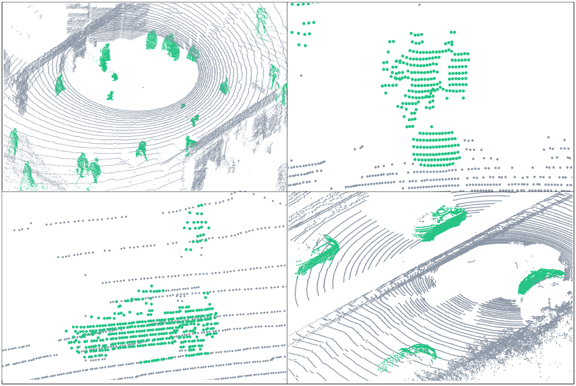

There is a need for a solution that offers accurate dynamic object detection for agents operating in diverse environments. To address this, we propose a novel MOS approach to accurately identify dynamic objects in point cloud data irrespective of the sensor characteristics, platform dynamics, and operating environments.

The contribution of this work is a low-configuration and learning-free approach to segmenting moving points from point cloud data. The foundation of the proposed approach lies in modelling each voxel using a hidden Markov model to exploit existing probabilistic frameworks for change-point detection tasks (James et al., 2024). For the application of labelling dynamic points, this amounts to identifying voxels that have changed occupancy. The change-point detection results are filtered using classical image processing techniques extended to point cloud data to reduce false positives and increase the performance recall by capturing the entire dynamic object. Integration of the ideas presented in this paper illustrates a simple MOS pipeline that (i) demonstrates strong generalized performance across platform dynamics (handheld, mobile robot, vehicle), sensor characteristics (Velodyne, Ouster, Livox, etc.), and sensing environments (indoor, outdoor, urban), while (ii) having a small and meaningful set of algorithm configuration parameters that remain unchanged for all experiments. In supporting the claims regarding the algorithm’s performance, we also highlight the loose definition of a moving object in the existing work and the variability in benchmarking MOS algorithms. The work is open-sourced at https://github.com/vb44/HMM-MOS to aid future development and provide reproducibility of all benchmarking results presented in this paper.

Challenges

Segmenting moving points in point cloud data is a challenging task. This Section discusses the uncertainty in the problem inputs, the challenge of providing generalized performance, meeting real-time performance requirements, and the diversity in the benchmark evaluations. Approaches to solving the MOS problem need to handle these challenges.

Handling uncertainty in the problem inputs

The MOS problem requires two inputs: a sequence of point cloud data, and the corresponding 6-DOF pose of the sensor.

Point cloud measurements are typically recorded using LiDAR sensors. LiDARs return a set of range measurements at specified heading and elevation angles at frequencies typically between 5 and 20 Hz. The sensors exhibit range measurement uncertainty that increases with distance. Additionally, the intrinsic parameters (beam heading, elevation angles) are only known to a level of uncertainty and require careful calibration to allow correct interpretation of the range measurement (Nouiraa et al., 2016).

Transforming the point cloud measurements into a frame relative to previous measurements (e.g. a map frame) requires accurate sensor pose estimation. The sensor’s pose is generally estimated by Global Navigation Satellite Systems (GNSS) or point cloud odometry, such as MOLA (Blanco-Claraco, 2024). These pose estimates inherently contain uncertainty, which, combined with the sensor’s measurement uncertainty, propagates in transforming the point cloud to the common reference frame. The effects are more pronounced at greater ranges, where pose errors result in substantial errors in the transformed measurements. Furthermore, if the platform’s pose solution and LiDAR are offset, as in the case of using GNSS for platform pose, accurate extrinsic calibration is required to locate the LiDAR relative to the navigation solution (D’Adamo et al., 2018).

LiDAR provides accurate range measurements at high frequencies but has known sensing limitations. Sensor measurements are sparse at long ranges, making it challenging to separate noisy detections from objects with only a few measurements. The behaviour of range returns from reflective surfaces is unpredictable and leads to incorrect beliefs about space occupancy, resulting in subsequent false detections. However, these surfaces are commonly encountered, and algorithms need to account for these sources of uncertainty. Sensor returns from vegetation and atmospheric obscurants such as dust also exhibit unpredictable behaviour (Phillips et al., 2017).

Providing real-time performance

Systems aim to provide detection results at rates commensurate with the cycle times of decision-making processes that consume the information. High-density scanners capture more information about the environment, but processing the increased measurements leads to greater computational demand. Modern LiDARs provide millions of measurements per second at high frequencies. Processing significant amounts of data in real-time applications requires hardware that is typically uncommon on mobile robots. Alternatively, the data volume can be reduced through pre-processing, but this generally introduces quantization and diminishes the level of detail in information about the scene.

Providing generalized performance

MOS has numerous applications ranging from robots interacting with humans (Falque et al., 2023) to vehicles navigating unstructured environments (Wojke and Häselich, 2012). An approach is desired that provides generalized performance across varying platform dynamics, sensor characteristics, and application environments. Learning-based approaches commonly fail to generalize performance between different sensors, platforms, and operational environments due to the large variation in the possible inputs. A common property of all sensors is the information provided about occupied and free space, and we use this to form confident beliefs about dynamic measurements.

Benchmarking metrics

Numerous labelled datasets are available for benchmarking the performance of MOS algorithms in comparison to existing methods. Each benchmark dataset includes a sequence of scans, in some cases the sensor’s estimated pose, and a set of labelled ground truth scans. A labelled ground truth scan provides a binary classification of static and dynamic points in the scan. These scans have either been annotated manually (Schmid et al., 2023), by a static map generation approach (Lim et al., 2023), a deep-learning network (Chen et al., 2022), or a combination of any. While numerous labelled datasets exist, the definition of a moving point varies significantly, leading to an inaccurate comparison between algorithms. This raises the question of what defines a moving object?

An object is moving if its pose is changing relative to a fixed reference frame, regardless of the object’s velocity and previous dynamic state. Given the k-th point cloud located in a fixed reference frame, for example, the map frame, sensor measurements corresponding to objects that are moving are classified as dynamic. The remaining measurements are static. Measurements corresponding to objects that (i) were moving and have stopped moving, (ii) move at a future instance (t = k + 1), or (iii) have the potential to move, are not dynamic objects given the earlier description.

This work focuses on detecting objects that are currently moving. We acknowledge the difficulty in generating ground-truth labels using experimental data, with labelling often capturing other instances.

Existing MOS solutions

Literature is rich with many learning-free and learning-based approaches for solving the MOS problem. Learning-free methods use traditional algorithmic approaches to identify dynamic points, compared to learning-based approaches that employ deep-learning networks to train models based on rules and verify performance on unseen datasets. The following discusses recent advancements in both categories. The reader is encouraged to view (Peng et al., 2024) for an in-depth review of dynamic object detection using point clouds.

Learning-free approaches

Learning-free approaches are generally categorized into methods identifying discrepancies between successive scans registered in a common frame and methods constructing a continuous representation of the environment updated sequentially with new observations. In common, these approaches query changes in free space to provide cues for detecting dynamic objects.

Scan-based

Scan-based methods compare observations to highlight discrepancies in the environment. Static points are likely to overlap when aligning successive point clouds, whereas dynamic points are likely to be misaligned in a common observed space. The discrepancies seed the detection of dynamic objects, with subsequent stages responsible for growing the region or rejecting them as noisy detections.

Underwood et al. (2013) detect changes between 3D scans by identifying discrepancies in the observed space, with points labelled dynamic if they are greater than a threshold distance from points in previously registered scans. Analogous to other methods, this relies on identifying the free space and finding instances that violate these constraints. Yoon et al. (2019) propose a multi-stage pipeline for complete object detection, consisting of a backward and forward free-space check between scans to identify dynamic points, a box filter to reject noisy estimates, and a final region growth algorithm to capture the entire dynamic object. Dynamic detection relies on selecting a suitable window size that allows sufficient displacement of the dynamic object – a characteristic that differs between object classes such as vehicles, cyclists, and pedestrians. Dewan et al. (2016) encounter similar problems, leading to suboptimal detection in multiclass scenarios. A simple approach examining changes in spatiotemporal normals to detect dynamic objects is presented by Falque et al. (2023), but only short-range detection results are provided in human-centric environments. M-detector by Wu et al. (2024) provide real-time detection of events from LiDAR point streams. The method is unique in its approach to the fast detection of diverse dynamic points using simple occlusion principles embedded in a three-module network consisting of event detection, clustering and region growth, and depth image construction and maintenance. Experimental results demonstrate agnosticity across operational environments. However, the algorithm is configured using 14 parameters dependent on the LiDAR’s characteristics.

Map-based

Map-based methods construct a representation of the environment and query changes in its state to identify dynamic objects. These approaches are commonly probabilistic and exploit the characteristics of a LiDAR’s beam to label space as free or occupied.

Modayil and Kuipers (2008) demonstrate this basic idea by constructing a confident static representation of the environment using a 2D LiDAR and believing that any changes in the environment must be due to dynamic objects. This belief keeps the detection object-agnostic, however, application to 3D point clouds in highly dynamic environments demonstrates below-par performance (Schmid et al., 2023). The Octomap probabilistic mapping framework by Hornung et al. (2013) uses maximum and minimum clamping on the occupancy and free probabilities to evolve beliefs in dynamic environments. These thresholds dictate the rate at which voxels change state and are not agnostic to objects with varying dynamics. Extensions to Octomap aim to improve its performance in dynamic environments, see Arora et al. (2021); Liu et al. (2023). Methods using similar techniques, such as clamping and forgetting policies described by Yguel et al. (2008), cannot adapt to different object classes to provide fast detection results without compromising the mapping quality and introducing significant false positive detections. Dynablox by Schmid et al. (2023) uses a Truncated Signed Distance Field (TSDF) map representation and integrates temporal properties to allow for motion detection and consequently construct a static map. The method builds a high-confidence spatiotemporal estimate of free space and identifies transitions between occupied and free space to seed dynamic objects. It demonstrates state-of-the-art performance in detecting dynamic objects in complex environments, as many learning-based approaches fail to generalize their detection capability to a broader class of dynamic objects. The algorithm is evaluated on various handheld human-centric datasets only.

Learning-based approaches

Most recent MOS approaches are learning-based. These methods use labelled data to train deep-learning networks that learn patterns to identify dynamic objects in point cloud data. The idea is to train these networks with sufficient high-quality labelled data to allow for accurate performance in unseen instances with variations in the input data quality, that is, sensor characteristics, sensor noise, and pose estimation uncertainty. The performance usually depends on the design of the network architecture and the quality of the labelled data used for training.

Convolutional Neural Networks (CNNs) frequently form the foundation of MOS deep-learning models. Chen et al. (2021) use sequential range images with a CNN to identify residuals in point clouds registered over a receding window to separate static and dynamic points. The algorithm performs accurately in scenarios similar to its training set but shows significantly reduced performance when evaluated with datasets collected with differing motion profiles and diverse dynamic objects. To improve the robustness of the network across applications, Mersch et al. (2022) employ spatiotemporal 4D convolutions combined with a binary Bayes filter for a recursive fusion of predictions over a receding horizon. This unique approach to training a CNN allows for significant improvements in the generalized performance across testing scenarios as the network trains to detect changes in a sequence of scans compared to appearance-based techniques. Mersch et al. (2023) extend this to include volumetric beliefs and increase dynamic detection while recursively updating a local static map of the environment. Wang et al. (2023) also uses 4D convolutions with instance detection and feature fusion to better identify static and dynamic objects in the scan.

Several other architecture designs also achieve accurate performance, including the use of dynamic graph CNNs (Wang and Solomon, 2021), leveraging semantic and motion labels in a range image-based CNN (Kim et al., 2022), and using a bird’s-eye view approach for motion detection (Zhou et al., 2023).

The critical hurdle involves generalizing performance across various operating environments and sensors with differing point cloud densities and scan patterns. The recently introduced HeLiMOS dataset by Lim et al. (2024) emphasizes the importance of generalization and provides labelled data from four different LiDARs along the same sequence. The performance of existing methods on the different LiDAR datasets without retraining highlights the poor generalized performance. Furthermore, the dependence on the training inputs and consequent variation in results reveals the gap for a robust approach to the MOS problem.

Identifying dynamic points using hidden Markov models

The MOS problem is defined as follows. Given,

(1) a sequence of N point clouds in the sensor frame $(\mathcal{S})$ , $P_{\mathcal{S}}=\{P_{\mathcal{S},1},\dots ,P_{\mathcal{S},N}\}$ , where each point cloud is a set of Cartesian measurements, $P_{\mathcal{S},k}=\{{\mathbf{p}}_1,\dots ,{\mathbf{p}}_r\}$ , ${\mathbf{p}}_i\in {\mathbb{R}}^3$ , and

(2) the corresponding pose estimates of the sensor in a map frame $(\mathcal{M})$ , $T_{\mathcal{M}\to \mathcal{S}}=\{{\mathbf{T}}_{\mathcal{M}\to \mathcal{S},1},\dots ,{\mathbf{T}}_{\mathcal{M}\to \mathcal{S},N}\}$ , ${\mathbf{T}}_{\mathcal{M}\to \mathcal{S},i}\in {\mathbb{R}}^{4\times 4}$ ,

the aim is to separate each point cloud into static and dynamic points, $\{P_{\mathcal{S},k}^{\text{static}}\cup P_{\mathcal{S},k}^{\text{dyn}}\}\subseteq P_{\mathcal{S},k}$ .

We treat the MOS task as a change-point detection problem, where the goal is to identify measurements in areas that have changed occupancy, that is, space transitioning from being free to occupied, and extend the dynamic detection to capture the entire object. James et al. (2024) presents an application-agnostic framework for modelling change-point detection tasks using hidden Markov models (HMMs). Hidden Markov models provide a strong probabilistic framework for handling uncertain observations and estimating a system’s true state. For the MOS task, this amounts to handling uncertain point cloud measurements and sensor pose estimates to infer the true occupancy of the voxel, and consequently, when it changes state. We adapt the framework presented by James et al. (2024) to model each voxel and update its occupancy based on uncertain observations. Meyer-Delius et al. (2012) and Wang et al. (2014) have previously used HMMs to model space occupancy for mapping tasks due to their fast adaptability to changes in the environment.

This section details the design of the proposed algorithm. Figure 2 illustrates the simple three-stage process for labelling dynamic measurements.

Figure 2.

The proposed approach uses a simple three-stage process to label dynamic measurements. The point cloud is first voxelized at a resolution of Δ, followed by a raycasting operation to determine all the observed voxels. Information about free and occupied space is described using a Gaussian distance field to generate the likelihood of each voxel being occupied or free. This information is used by the HMM filter to probabilistically update the occupancy of each voxel. The local map is queried to detect voxels that have transitioned occupancy. These changes are filtered using a spatiotemporal convolution to decrease incorrect detections and capture the entire object. The methodology details each submodule.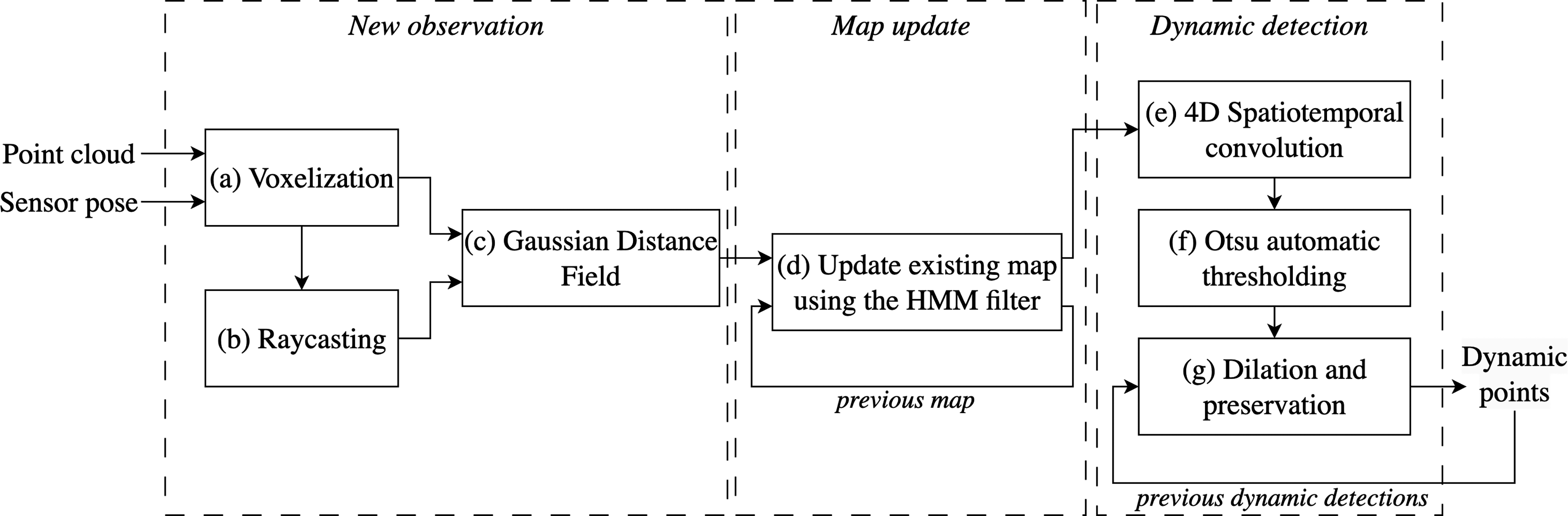

Map representation and update

A global map frame, $\mathcal{M}$ , is defined to indicate the origin of the environment, commonly located at the origin of the first scan. At time k, the map, $M_{\mathcal{M},k}$ , is discretized using voxels, v, of a user-configured size, Δ. The voxels are augmented with properties alongside their position to model spatiotemporal behaviour. The properties are summarized in Figure 3 and detailed throughout this section.

Figure 3.

Each voxel, v _i , has several properties augmented with its discretized position (x _i , y _i , z _i ) to provide temporal information for detecting state changes.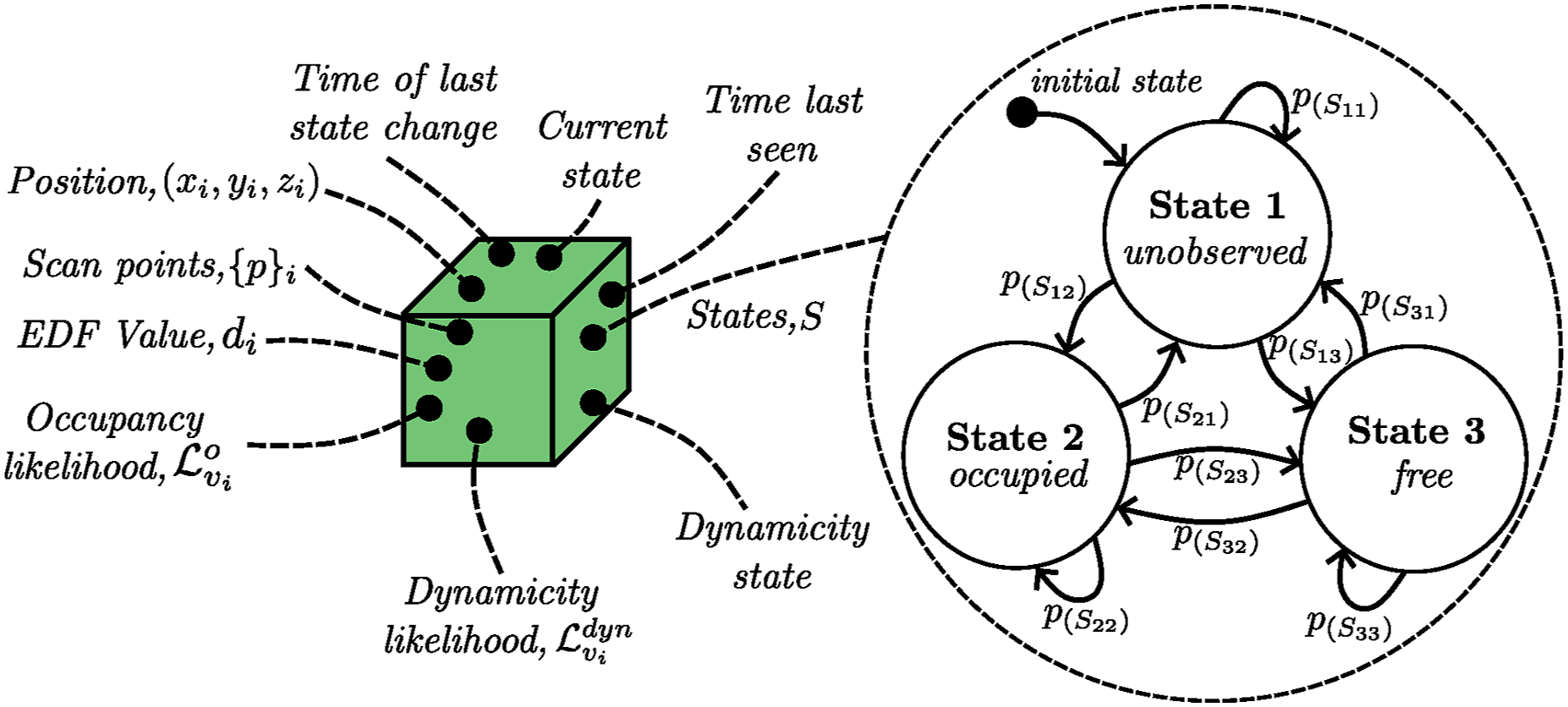

Without uncertainty, detecting dynamic objects is as simple as updating voxel occupancy with new observations. If a voxel’s state changes from free to occupied, it suggests a dynamic measurement. However, uncertainties in point cloud measurements, sensor pose, or poor sensing conditions lead to incorrect or missed detections. Existing beliefs should be fused probabilistically to handle the various sources of uncertainty. As the state of each voxel is not directly interpretable due to the associated uncertainty, an HMM is used to represent the state of each voxel in the map, $M_{\mathcal{M},k}$ .

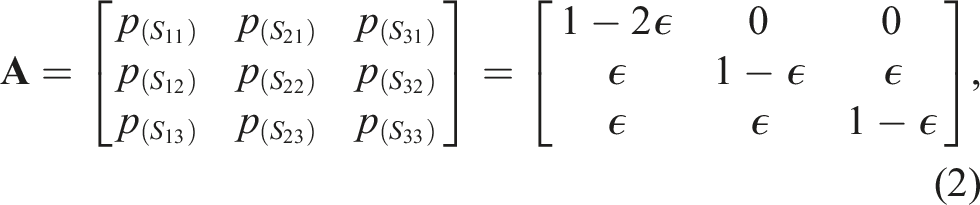
Representing each voxel using an HMM (Rabiner, 1989) requires defining: the n states of the voxel, S = {S₁, …, S _n }, the transition probabilities between the states captured in the state transition matrix $\mathbf{A}\in {\mathbb{R}}^{n\times n}$ , and a process to generate the likelihood of the i-th voxel being in each state at time k given the sensor observations, encoded in the measurement conditional densities, ${\mathbf{B}}_{i,k}\in {\mathbb{R}}^{n\times n}$ . Let the i-th voxel’s state vector, ${\widehat{\mathbf{x}}}_{i,k}\in {\mathbb{R}}^{n\times 1}$ , denote the probability of being in each state at time k. The voxel’s initial state is given in ${\widehat{\mathbf{x}}}_{i,0}$ . Once defined, a voxel’s state is efficiently updated using the recursive HMM filter (Elliott et al., 2008),

${\widehat{\mathbf{x}}}_{i,k}={\eta }_{i,k}{\mathbf{B}}_{i,k}\mathbf{A}{\widehat{\mathbf{x}}}_{i,k-1},$

(1)

where η_i,k is a normalization factor that ensures ${\widehat{\mathbf{x}}}_{i,k}$ is a probability. The current state depends only on the previous state and the new observation. Using an HMM to represent each voxel provides a probabilistic approach to integrating new information into an existing map. Figure 2(d) shows the map update step in reference to the proposed pipeline.

Each voxel, v, is represented using three states (n = 3), S = {unobserved, occupied, free}, with each voxel initialized in the unobserved state, ${\widehat{\mathbf{x}}}_{i,0}={\left[\begin{array}{ccc}\hfill 1\hfill & \hfill 0\hfill & \hfill 0\hfill \end{array}\right]}^{\text{T}}$ . The state transitions are set as

$\mathbf{A}=\left[\begin{array}{ccc}\hfill p_{(S_{11})}\hfill & \hfill p_{(S_{21})}\hfill & \hfill p_{(S_{31})}\hfill \\ \hfill p_{(S_{12})}\hfill & \hfill p_{(S_{22})}\hfill & \hfill p_{(S_{32})}\hfill \\ \hfill p_{(S_{13})}\hfill & \hfill p_{(S_{23})}\hfill & \hfill p_{(S_{33})}\hfill \end{array}\right]=\left[\begin{array}{ccc}\hfill 1-2ϵ\hfill & \hfill 0\hfill & \hfill 0\hfill \\ \hfill ϵ\hfill & \hfill 1-ϵ\hfill & \hfill ϵ\hfill \\ \hfill ϵ\hfill & \hfill ϵ\hfill & \hfill 1-ϵ\hfill \end{array}\right],$

(2)

where ϵ is an algorithm configuration parameter, set to ϵ = 0.005 for the MOS task. The transition probabilities are selected on the belief that a voxel is likely to stay in its current state and requires sufficient confidence before transitioning. Once a voxel is observed as either occupied or free, it cannot transition back to the unobserved state using the voxel update process, as indicated by the zeros in the first row. The voxels are only reset to State one when maintaining the map size. The map size is maintained by (i) pruning voxels outside the sensor’s maximum range, r_max, and (ii) voxels that have not been unobserved in a global receding window, set as a configuration parameter w _g . The parameter r_max is configured by hardware or set by the requirement for detecting dynamic objects within a specified range. The global window is introduced to limit the effect of developing incorrect beliefs from drift in the sensor pose estimates.

Interpretation of a new observation

The new point cloud at time k in the sensor frame, $P_{\mathcal{S},k}$ , is transformed by the current sensor pose estimate, ${\mathbf{T}}_{\mathcal{M}\to \mathcal{S},k}$ , to locate the scan points in the map frame,

$P_{\mathcal{M},k}={\mathbf{T}}_{\mathcal{M}\to \mathcal{S},k}{P}_{\mathcal{S},k}.$

(3)

The scan in map frame, $P_{\mathcal{M},k}$ , is discretized at a voxel resolution of Δ, to form a voxelized scan, $P_{\mathcal{M},k}^{\prime }=\{v_1,\dots ,v_j\}$ (Figure 2(a)). A raycasting operation is performed from the sensor’s position to all voxelized measurements in $P_{\mathcal{M},k}^{\prime }$ to determine the voxels observed by this scan. All observed voxels are saved in $P_{\mathcal{M},k}^{\prime \mathrm{o}\mathrm{b}\mathrm{s}}$ (Figure 2(b)). The discretized raycast operation is performed efficiently using the line algorithm by Bresenham (1965).

The interpretation of the current scan provides information about occupied and free voxels. However, believing the information and overwriting previous beliefs directly generates suboptimal results, as uncertainty leads to a rapid transition of voxels between occupied and free states. This is problematic as the main cue used for dynamic detection is the transition of previously free voxels turning occupied. Instead, the likelihood of each observed voxel being free and occupied is used to construct a belief of the current state of the voxel. The measurement conditional densities of the i-th voxel being in a particular state given an observation are

${\mathbf{B}}_{i,k}=\text{diag}(0,{\mathcal{L}}_{v_i}^o,1-{\mathcal{L}}_{v_i}^o),$

(4)

where ${\mathcal{L}}_{v_i}^o$ is the likelihood of the voxel being occupied.

An observed voxel is likely to be occupied if it is close to a voxel in the voxelized scan, $P_{\mathcal{M},k}^{\prime }$ . Similarly, an observed voxel is likely to be free if it is distant from a voxel in the voxelized scan. This information can be captured using a Gaussian Distance Field (GDF), which is derived from the commonly used Euclidean Distance Field (EDF) (Oleynikova et al., 2016) (Figure 2(c)). First, an EDF is constructed for the current scan. Figure 4 shows an example. For each observed voxel, $v_i\in P_{\mathcal{M},k}^{\prime \mathrm{o}\mathrm{b}\mathrm{s}}$ , the closest distance, d _i , to the nearest voxel in the voxelized scan, $v_j\in P_{\mathcal{M},k}^{\prime }$ , is computed and augmented to voxel v _i ’s properties. This Euclidean distance is used to calculate the likelihood of being in each state by evaluating an unnormalized Gaussian function at d _i ,

${\mathcal{L}}_{v_i}^o=\exp \left(-d_i^2/\left(2{\sigma }_o^2\right)\right),$

(5)

where σ _o is a user-configured standard deviation to capture the uncertainty in the estimate. The standard deviation represents a lumped uncertainty of locating the point cloud measurements in the map frame. If the standard deviation is zero, the beliefs are directly integrated into the existing map, and each voxel is modelled as a Markov model. Alternatively, uncertainty propagation methods can be used if the uncertainty in the point cloud measurements and sensor pose can be estimated. This allows for more realistic uncertainty modelling of the point cloud measurements, as uncertainty is known to increase with range. The lumped uncertainty provides a simple implementation where these uncertainties cannot be estimated explicitly. These likelihoods are used to construct the measurement conditional densities in equation (4), and integrate the new observation into the existing map using the HMM filter described in equation (1).

Figure 4.

A voxelized scan is shown on the left, captured by the LiDAR at the origin. The computed Euclidean Distance Field (EDF) of the point cloud is shown on the right. The EDF values are transformed by a Gaussian function to compute an occupancy likelihood. Voxels close to occupied measurements are likely to be occupied, and voxels located away are more likely to be free.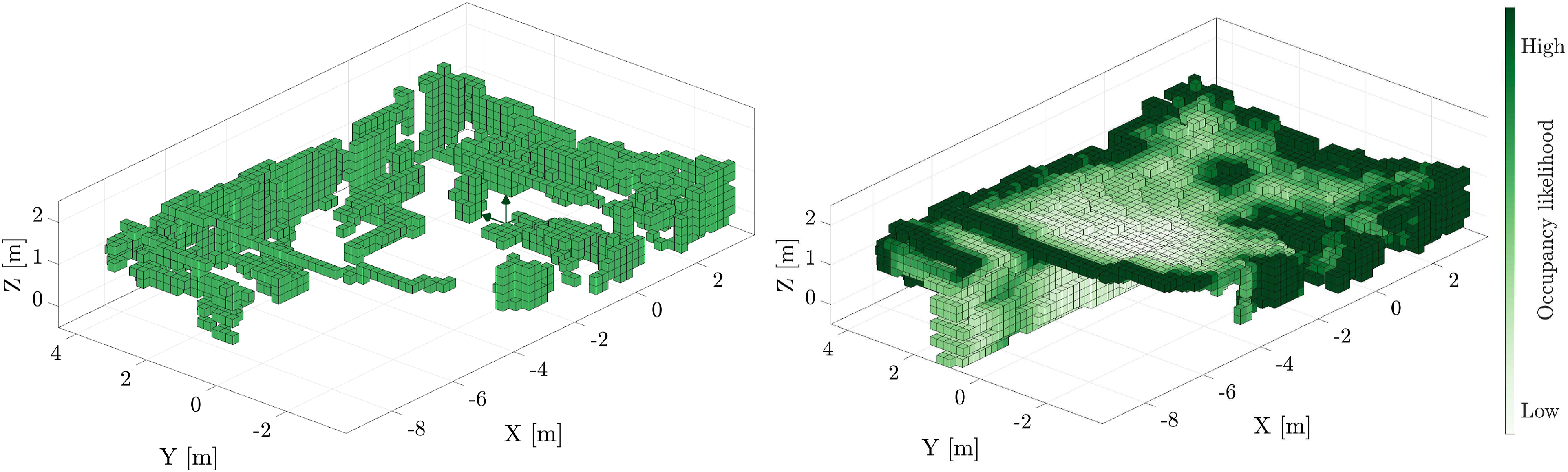

A voxel’s current state, S_i,k, is updated when the probability of being in a particular state, x_i,k, is greater than a predefined threshold, p_min, else, the voxel remains in the previous state,

$S_{i,k}=S\left.\left(\underset{i}{\mathrm{a}\mathrm{r}\mathrm{g}\mathrm{m}\mathrm{a}\mathrm{x}}({\widehat{\mathbf{x}}}_{i,k})\right)\right|\max ({\widehat{\mathbf{x}}}_{i,k})>p_{\text{min}}.$

(6)

Dynamic point identification

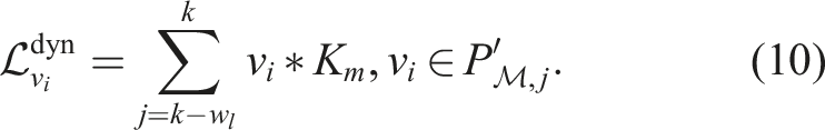
This process allows for an efficient probabilistic update of each voxel’s state in the global map. A voxel’s transition between free and occupied space is used to seed the detection of dynamic objects. The HMM per voxel allows for an accumulation of confidence before transitioning state. Figure 5 illustrates the process of estimating dynamic voxels with the following detailing each step.

Figure 5.

A 4D convolution is performed to capture spatial and temporal changes. The figure illustrates an example of performing a spatial convolution on a voxelized point cloud after detecting changes in the voxel’s state. Voxels that have changed state are shown in dark green. An example kernel (red), K₃, is convolved with the point cloud to identify missed detections and suppress noisy estimates. The convolution is temporally extended across a local window of w _l to calculate the likelihood of each voxel being dynamic, 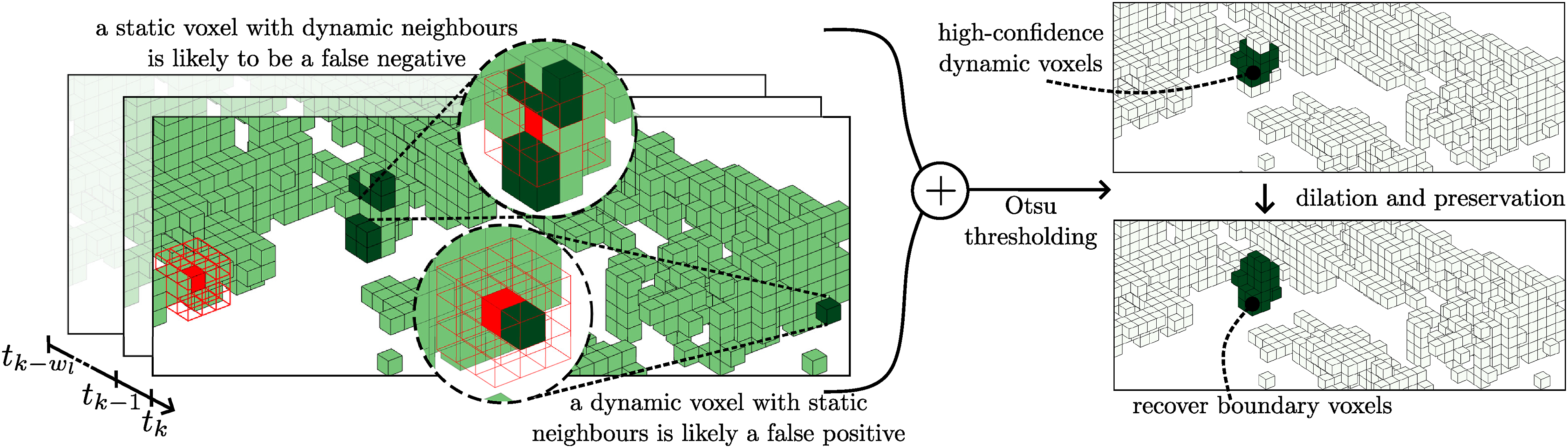${\mathcal{L}}_{v_i}^{\text{dyn}}$ . Dynamic voxels are separated using Otsu’s automatic thresholding, and previously identified dynamic voxels and a nearest-neighbour dilation are used to capture the complete object. The figure is best viewed in colour.

Detecting changes in voxel states

The first step is to identify voxels from the current voxelized scan, $P_{\mathcal{M},k}^{\prime }$ , that changed state in the updated voxel map, $M_{\mathcal{M},k}$ ,

$\begin{array}{c}\hfill P_{\mathcal{M},k}^{\prime \mathrm{c}\mathrm{h}\mathrm{g}}=\left\{\left.v_i\in P_{\mathcal{M},k}^{\prime }\right|S_{i,k}\ne S_{i,k-1}\text{\hspace{0.17em}and\hspace{0.17em}}{S}_{i,[k-1,k]}\ne S_1\right\}.\end{array}$

(7)

Transitions to and from the unobserved state (S₁) are neglected as these are new observations. The resulting subset of voxels, $P_{\mathcal{M},k}^{\prime \mathrm{c}\mathrm{h}\mathrm{g}}\subset P_{\mathcal{M},k}^{\prime }$ , contain true and false dynamic detections.

Capturing neighbourhood behaviour using a spatiotemporal (4D) convolution

The change detection allows for likely dynamic voxels to be identified. However, each voxel is modelled independently, and changes in the voxel’s neighbourhood are not examined. Dynamic objects are likely to occupy space composed of several voxels, given a sufficiently small discretization resolution. Two heuristics can be stated without assuming the object’s shape or dynamics to keep the algorithm application agnostic; (i) a static voxel with many dynamic neighbours is likely a missed detection (false negative), and (ii) a dynamic voxel with many static neighbours is likely a false detection (false positive). A spatial (3D) convolution is performed to identify missed detections to reduce the false negatives and suppress noisy detections to decrease false positives.

While both heuristics significantly improve the results, they do introduce unwanted effects. As a consequence of heuristic (i), detections at sparse, and often long ranges, are missed as they exhibit similar behaviour to noisy measurements. Heuristic (ii) captures parts of static objects when a dynamic object moves close to static parts of the environment. This depends on the voxel size, as it is common for a voxel to capture both static and dynamic parts of the environment (e.g. feet and wheels contacting the ground). The benefits of performing the convolution significantly outweigh the unwanted side effects.

For each occupied voxel, $v_i\in P_{\mathcal{M},k}^{\prime }$ , the likelihood of being dynamic, ${\mathcal{L}}_{v_i}^{\text{dyn}}$ , is calculated by summing state changes in the voxel’s local neighbourhood. A kernel, $K_m\in {\mathbb{R}}^{m\times m\times m}$ , is convolved with each voxel in $P_{\mathcal{M},k}^{\prime }$ to compute the likelihood of the voxel being dynamic,

$\begin{array}{cc}\hfill {\mathcal{L}}_{v_i}^{\text{dyn}}& =v_i\ast K_m,v_i\in P_{\mathcal{M},k}^{\prime }\hfill \\ \hfill & =\text{max}\left(\sum \alpha (v_j)\forall v_j\in K_m(v_i),0\right),\hfill \end{array}$

(8)

where α(v _j ) is given by

$\begin{array}{c}\hfill \alpha (v_j)=\left\{\begin{array}{cc}1,\hfill & \text{if}{v}_j\in P_{\mathcal{M},k}^{\prime \mathrm{c}\mathrm{h}\mathrm{g}}\cap S(v_j)\ne S_1,\hfill \\ 0,\hfill & \text{else\hspace{0.17em}if}{v}_j\notin P_{\mathcal{M},k}^{\prime \mathrm{c}\mathrm{h}\mathrm{g}}\cap S(v_j)\ne S_1,\hfill \\ -1,\hfill & \text{otherwise}.\hfill \end{array}\right.\end{array}$

(9)

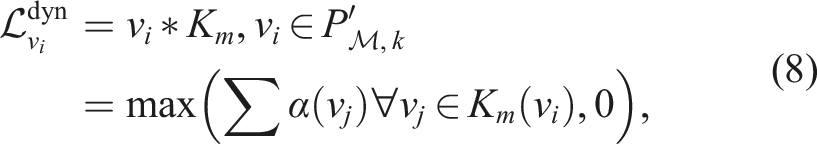
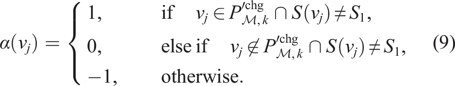
The condition, S(v _j ) ≠ S₁, is added to avoid including detections that are close to the boundary between unobserved (S₁) and observed (S₂, S₃) space, as voxelization is known to be inaccurate at this boundary. A dynamic detection close to this boundary is penalized as in the third constraint of equation (8) to allow for the detection of high-confidence dynamic voxels only. Voxels missed due to this constraint are recovered in the final step of the pipeline. The likelihood of being dynamic increases with the number of voxels in the convolution kernel, K _m , that have changed state. A post-processing local neighbourhood median filter is also applied to smooth the likelihood values.

The spatial 3D convolution (equation (8)) is extended over a receding local window of size w _l , to compute a spatiotemporal 4D convolution,

${\mathcal{L}}_{v_i}^{\text{dyn}}=\sum _{j=k-w_l}^k{v}_i\ast K_m,v_i\in P_{\mathcal{M},j}^{\prime }.$

(10)

The addition of the temporal convolution over w _l allows for further suppression of incorrect detections. For example, a dynamic detection in one scan and static in the remaining scans reduces the likelihood of that voxel being dynamic. At the end of this stage, all voxels in $P_{\mathcal{M},j}^{\prime }$ have been assigned a likelihood of being dynamic (Figure 2(e)).

Automatic thresholding the 4D convolution

The spatiotemporal convolution assigns a high likelihood for dynamic voxels and a low likelihood for static voxels. The likelihood of a voxel being dynamic depends on many factors: the voxel size, Δ; the size of the convolution kernel, K _m ; the sparsity of the original point cloud, $P_{\mathcal{S},k}$ ; and the shape, size, and speed of the moving object. It is difficult to manually set a threshold to separate voxels into static and dynamic classes based on their likelihood. The automatic thresholding algorithm by Otsu (1979), commonly used in image processing, is applied to the convolution scores to compute a dynamic threshold, γ, that provides a binary distinction between static and dynamic voxels (Figure 2(f)). A lower bound on the threshold, γ_min, is required as the algorithm continues to provide separation for static scans due to the presence of noisy detections,

$P_{\mathcal{M},k}^{\prime \mathrm{d}\mathrm{y}\mathrm{n}}=\{v_i\in P_{\mathcal{M},k}^{\prime }|{\mathcal{L}}_{v_i}^{\text{dyn}}>\max (\gamma ,{\gamma }_{\text{min}})\}.$

(11)

It is important to mention that this only estimates the high-confidence dynamic voxels. The lower threshold, γ_min, corresponds to the minimum number of dynamic neighbours of voxel v _i in its neighbourhood defined by the kernel size K _m in the local window, w _l .

Preserving high-confidence dynamic voxels and extending to low-confidence areas

High-confidence dynamic voxels from the previous scan are preserved in the current scan (Figure 2(g)). The recursive preservation is independent of the receding window, w _l , used in previous operations. This aims to help capture the complete object. All dynamic predictions from the previous scan are not preserved, as these may contain false positive detections. Instead, only voxels with a likelihood of being dynamic, ${\mathcal{L}}_{v_i}^{\text{dyn}}$ , greater than the minimum threshold, γ_min, are included,

$P_{\mathcal{M},k}^{\prime \mathrm{d}\mathrm{y}\mathrm{n}}=P_{\mathcal{M},k}^{\prime \mathrm{d}\mathrm{y}\mathrm{n}}\cup \{v_i\in P_{\mathcal{M},k-1}^{\prime \mathrm{d}\mathrm{y}\mathrm{n}}|{\mathcal{L}}_{v_i}^{\text{dyn}}>{\gamma }_{\text{min}}\}.$

(12)

This helps to preserve only the high-confidence predictions.

A nearest-neighbour dilation is applied to the high-confidence voxels to grow the dynamic detection results into neighbouring regions (Figure 2(g)), which were previously disregarded due to strict constraints to avoid identifying false positives,

$P_{\mathcal{M},k}^{\prime \mathrm{d}\mathrm{y}\mathrm{n}}=P_{\mathcal{M},k}^{\prime \mathrm{d}\mathrm{y}\mathrm{n}}\cup \{v_i\in P_{\mathcal{M},k}^{\prime }|\exists v_j\in K_3(v_i):v_j\in P_{\mathcal{M},k}^{\prime \mathrm{d}\mathrm{y}\mathrm{n}}\}.$

(13)

The final step involves extracting the original point cloud measurements from $P_{\mathcal{S},k}$ that are captured in $P_{\mathcal{M},k}^{\prime \mathrm{d}\mathrm{y}\mathrm{n}}$ , and labelling them as being $P_{\mathcal{S},k}^{\text{static}}$ or $P_{\mathcal{S},k}^{\text{dyn}}$ .

Summary

Using HMMs provides a probabilistic approach to modelling the environment while extending image processing techniques to point cloud data filters the dynamic detections. The proposed approach uses a simple pipeline composed of three stages: (i) voxelizing a new scan, (ii) probabilistically integrating the new scan into the existing map, and (iii) detecting changes in the environment’s state using spatiotemporal (4D) convolutions. Table 1 provides a complete listing of the algorithm’s configuration parameters.

Table 1.

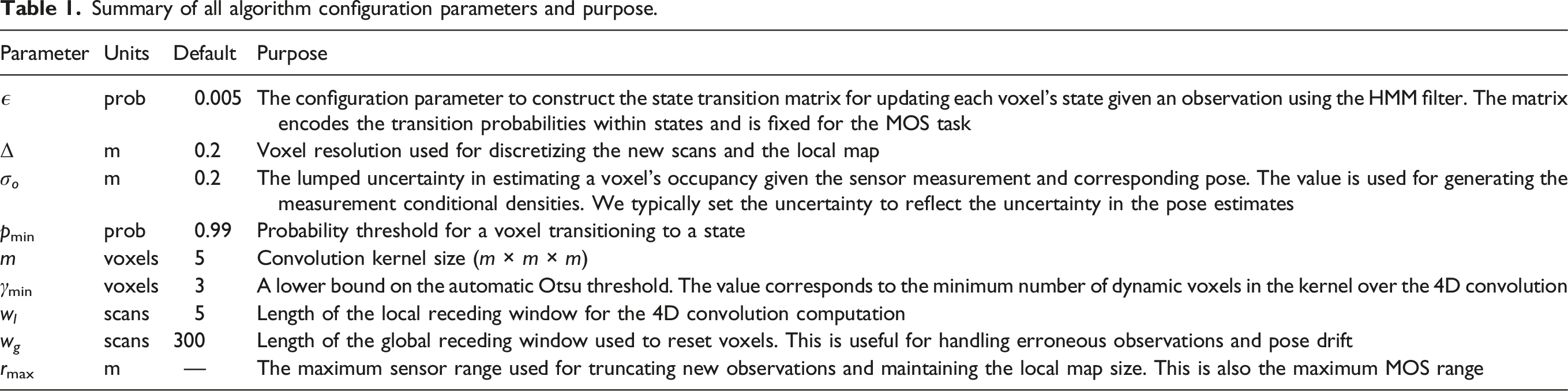
Summary of all algorithm configuration parameters and purpose.

Parameter	Units	Default	Purpose
ϵ	prob	0.005	The configuration parameter to construct the state transition matrix for updating each voxel’s state given an observation using the HMM filter. The matrix encodes the transition probabilities within states and is fixed for the MOS task
Δ	m	0.2	Voxel resolution used for discretizing the new scans and the local map
σ o	m	0.2	The lumped uncertainty in estimating a voxel’s occupancy given the sensor measurement and corresponding pose. The value is used for generating the measurement conditional densities. We typically set the uncertainty to reflect the uncertainty in the pose estimates
p min	prob	0.99	Probability threshold for a voxel transitioning to a state
m	voxels	5	Convolution kernel size (m × m × m)
γ min	voxels	3	A lower bound on the automatic Otsu threshold. The value corresponds to the minimum number of dynamic voxels in the kernel over the 4D convolution
w l	scans	5	Length of the local receding window for the 4D convolution computation
w g	scans	300	Length of the global receding window used to reset voxels. This is useful for handling erroneous observations and pose drift
r max	m	—	The maximum sensor range used for truncating new observations and maintaining the local map size. This is also the maximum MOS range

Results

The proposed algorithm’s performance is evaluated using publicly available benchmark datasets. Table 2 summarizes the benchmark datasets used for evaluating performance in comparison to existing methods. The different types of ground truth labelling approaches, type (I) to type (IV), are defined in the table and referred to throughout the results. The proposed approach is designed to label moving objects only, corresponding to type (I) labelling. Table 3 lists the different characteristics of the LiDARs used in the benchmark datasets. Results from published approaches are used where available or evaluated using the open-source package using the default configuration to test generalization capability. We do not retrain the networks with new data and use the provided weights for learning-based approaches, such as LMNet (Chen et al., 2021), 4DMOS (Mersch et al., 2022), MapMOS (Mersch et al., 2023), InsMOS (Wang et al., 2023), and MotionBEV (Zhou et al., 2023), to test the generalization performance across datasets. All approaches use the SemanticKITTI dataset for training. This Section concludes with a case study to demonstrate the performance of the proposed approach in comparison to other methods in a safety-critical application.

Table 2.

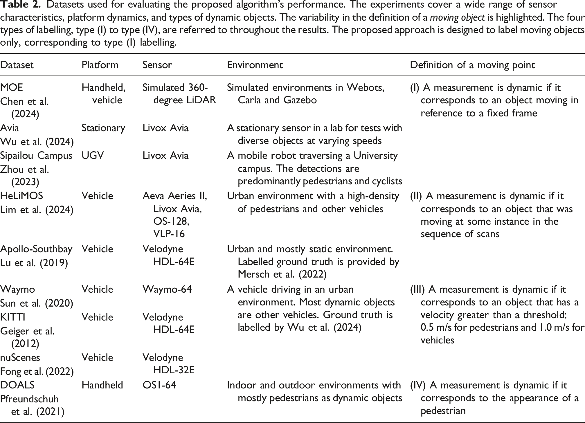
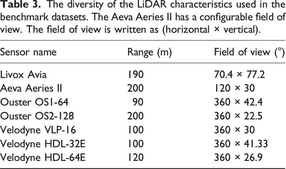
Datasets used for evaluating the proposed algorithm’s performance. The experiments cover a wide range of sensor characteristics, platform dynamics, and types of dynamic objects. The variability in the definition of a moving object is highlighted. The four types of labelling, type (I) to type (IV), are referred to throughout the results. The proposed approach is designed to label moving objects only, corresponding to type (I) labelling.

Dataset	Platform	Sensor	Environment	Definition of a moving point
MOE	Handheld, vehicle	Simulated 360-degree LiDAR	Simulated environments in Webots, Carla and Gazebo	(I) A measurement is dynamic if it corresponds to an object moving in reference to a fixed frame
Chen et al. (2024)
Avia	Stationary	Livox Avia	A stationary sensor in a lab for tests with diverse objects at varying speeds
Wu et al. (2024)
Sipailou Campus	UGV	Livox Avia	A mobile robot traversing a University campus. The detections are predominantly pedestrians and cyclists
Zhou et al. (2023)
HeLiMOS	Vehicle	Aeva Aeries II, Livox Avia, OS-128, VLP-16	Urban environment with a high-density of pedestrians and other vehicles	(II) A measurement is dynamic if it corresponds to an object that was moving at some instance in the sequence of scans
Lim et al. (2024)
Apollo-Southbay	Vehicle	Velodyne HDL-64E	Urban and mostly static environment. Labelled ground truth is provided by Mersch et al. (2022)
Lu et al. (2019)
Waymo	Vehicle	Waymo-64	A vehicle driving in an urban environment. Most dynamic objects are other vehicles. Ground truth is labelled by Wu et al. (2024)	(III) A measurement is dynamic if it corresponds to an object that has a velocity greater than a threshold; 0.5 m/s for pedestrians and 1.0 m/s for vehicles
Sun et al. (2020)
KITTI	Vehicle	Velodyne HDL-64E
Geiger et al. (2012)
nuScenes	Vehicle	Velodyne HDL-32E
Fong et al. (2022)
DOALS	Handheld	OS1-64	Indoor and outdoor environments with mostly pedestrians as dynamic objects	(IV) A measurement is dynamic if it corresponds to the appearance of a pedestrian
Pfreundschuh et al. (2021)

Table 3.

The diversity of the LiDAR characteristics used in the benchmark datasets. The Aeva Aeries II has a configurable field of view. The field of view is written as (horizontal × vertical).

Sensor name	Range (m)	Field of view (°)
Livox Avia	190	70.4 × 77.2
Aeva Aeries II	200	120 × 30
Ouster OS1-64	90	360 × 42.4
Ouster OS2-128	200	360 × 22.5
Velodyne VLP-16	100	360 × 30
Velodyne HDL-32E	100	360 × 41.33
Velodyne HDL-64E	120	360 × 26.9

We excluded the widely used Semantic KITTI dataset by Behley et al. (2019) from our analysis due to inaccuracies in its point cloud data collection and deskewing processes. These errors significantly misrepresent the performance of approaches that depend on accurate occupancy and free space information from the point cloud. This exclusion highlights a critical issue: datasets with acquisition flaws can lead to misleading algorithm evaluations and potentially skew research directions. Learning-free methods seem particularly vulnerable to such data inconsistencies, as they cannot compensate through ‘training’ for errors in spatial representation.

The proposed algorithm uses the default configuration listed in Table 1 for all tests. The testing is performed on an Intel i5 CPU with 14.9 GiB of memory running Ubuntu 20.04.6 LTS. Real-time processing relies on CPU threading only, implemented using Intel’s open-source Thread Building Blocks API (Intel, 2025). All results are reproducible using the instructions on the open-source page.

The algorithm’s performance is benchmarked using the Intersection over Union (IoU %) metric (Everingham et al., 2010),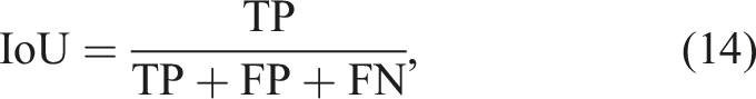

$\mathrm{I}\mathrm{o}\mathrm{U}=\frac{\mathrm{T}\mathrm{P}}{\mathrm{T}\mathrm{P}+\mathrm{F}\mathrm{P}+\mathrm{F}\mathrm{N}},$

(14)

where TP is the number of true positives, FP is the number of false positives, and FN is the number of false negatives. Each benchmark varies in the calculation of the IoU for a given sequence. For example, Dynablox uses the average IoU over the labelled scans, whereas HeLiMOS and the datasets released by M-detector accumulate the number of TP, FP, and FN over all scans and compute the IoU at the end only. All testing and evaluation conditions are detailed below for each dataset.

The proposed approach is compared to several existing approaches. 4DMOS by Mersch et al. (2022) is a state-of-the-art MOS approach that only uses a limited history of past scans to detect moving objects. Online and delayed results are provided. The delayed results fuse scans within a delayed window to estimate dynamic points. The published MapMOS (Mersch et al., 2023) results provide two variants as well: (i) dynamic object predictions using the current scan and (ii) dynamic object predictions using a volumetric belief that includes a delay of 10 scans. MapMOS retains a history of objects that transition from being dynamic to static, and hence demonstrates strong performance in datasets that label the ground truth accordingly. M-detector by Wu et al. (2024) do not benchmark using any of the existing baselines and alternatively releases ground-truth labels for datasets to only capture objects that are moving as per their definition. Dynablox by Schmid et al. (2023) only provide quantitative results for the DOALS dataset.

All methods use point cloud data provided in the sensor’s frame. 4DMOS and MapMOS use KISS-ICP (Vizzo et al., 2023) internally to estimate the sensor’s pose. M-detector uses FAST-LIO (Xu and Zhang, 2021) to estimate the sensor’s pose and does not publish the relevant poses with its labelled datasets. Deskewed scans (similar to KITTI) are used where possible, such as the HeLiMOS dataset.

Performance benchmarking

The following evaluates the algorithm’s performance on nine datasets to support the claims of providing generalized performance across platform dynamics, sensor characteristics, and operating environments while using the same algorithm configuration. Results for two different voxel sizes are included, Δ = 0.2 m and Δ = 0.25 m, with corresponding lumped uncertainties of σ _o = 0.2 m and σ _o = 0.25 m. While the accuracy results are similar, a significant computational benefit is achieved using the slightly larger voxel size. A trend is observed in some results where the larger voxel size returns a better result as it captures the complete object, however, this is usually at the expense of increasing false positives. This is a consequence of the quantization. The average runtime of each dataset is detailed in the corresponding section. A comparison with existing methods is provided when runtime results are published by the corresponding method or the open-source package results are reproducible. The reader’s attention is drawn to the variability in the ground truth of the benchmark datasets.

Moving event dataset (MOE)

The MOE dataset by Chen et al. (2024) provides a series of simulated and real-life sequences consisting of various diverse dynamic objects aimed at improving moving event detection using LiDAR sensors. Simulation datasets are beneficial as the sensor’s pose and the MOS labels are known. The authors benchmark existing algorithms on three simulated sequences: Sequence 00 is a mobile robot exploring an indoor apartment with humans as dynamic objects in the Webots simulator, sequence 01 is an outdoor city scene traversed by a vehicle in the Carla simulator, and sequence 02 is recorded in a crowded pedestrian setting in the Gazebo simulator. Table 4 shows the published benchmark updated with the method proposed in this paper. The proposed algorithm performs consistently for all sequences, providing the best results for sequences 00 and 02. The benchmark uses the mean of the per-scan IoU metric for benchmarking performance, which is sensitive to the number of dynamic detections per scan. Most other benchmarks in this section use the total IoU, which provides a total sum of the dynamic detections for the entire sequence, reducing the sensitivity compared to the mean IoU.

Table 4.

Evaluation on the MOE dataset with best results in bold. 4DMOS and MapMOS were evaluated using their open-source packages, with the delayed results separated at the bottom of the table. Results for all other methods are as documented by Chen et al. (2024). The ground truth uses type (I) labelling.

Method	Sequence IoU (%)
	00	01	02
Removert	29.7	2.8	42.1
ERASOR	37.8	2.8	62.7
Octomap	32.8	3.1	65.2
Dynablox	32.0	19.5	49.2
DOD	78.6	14.2	59.5
M-detector	30.5	17.4	4.4
MotionBEV	0.2	5.5	6.9
InsMOS	49.5	28.2	37.9
4DMOS, online	71.2	26.1	66.0
This paper Δ = 0.20 m	80.0	38.2	81.9
This paper Δ = 0.25 m	70.6	40.5	77.6
4DMOS, delayed	78.0	25.7	76.2
MapMOS, volume	27.8	50.3	78.7

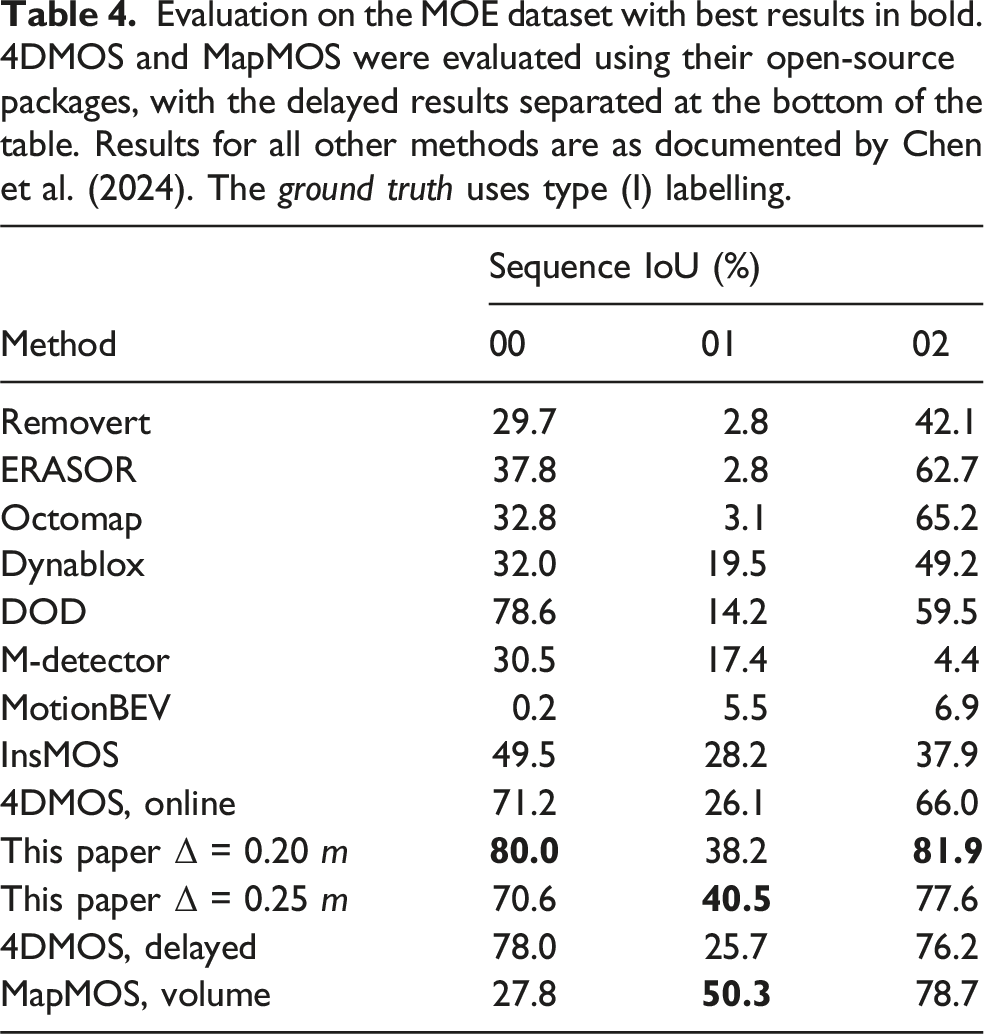
Sequences 00 and 02 are processed at 40 Hz for a maximum 50 m MOS range, whereas sequence 01 processes at 10 Hz for a maximum 20 m range and 3 Hz for a 50 m range. Sequences 00 and 02 are indoor environments, providing dense scans with a low maximum range, whereas sequence 01 is recorded in an outdoor environment with dense long ranges. The per-frame computation is proportional to the number of measurements (scanning density) and the scanning range. This relationship is observed for all datasets. The algorithm does not discard measurements that are greater than the configured maximum range. Instead, the ray is truncated at the maximum range to accurately model free space.

HeLiMOS

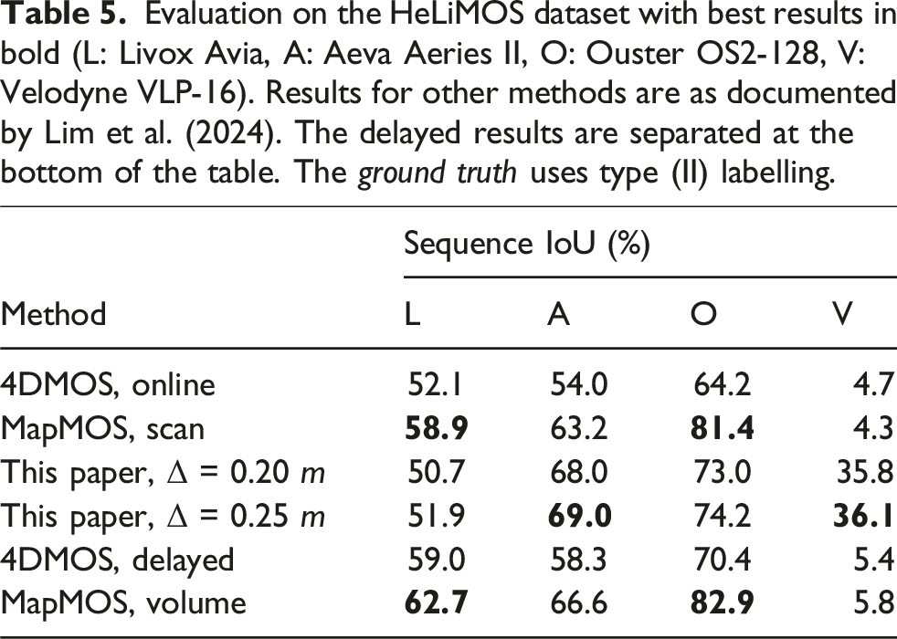
The HeLiMOS dataset provides the ground-truth labels for a single sequence from the HeLiPR dataset (Jung et al., 2024) captured simultaneously by four LiDARs: a Livox Avia, an Aeva Aeries II, a Velodyne VLP-16, and an Ouster OS2-128. The dataset is unique in highlighting the importance of sensor-agnostic MOS, with the purpose of providing consistent performance independent of the sensor used to generate the point cloud data. We achieve consistent performance across all sensors as demonstrated in Figure 6 and Table 5. The sensor pose is estimated using SiMpLE (Bhandari et al., 2024). 4DMOS and the proposed approach provide instantaneous detection of dynamic objects and use a small temporal history only, whereas MapMOS predicts all moving objects, even when they transition to being static. We outperform 4DMOS in all scenarios, except for the Aeva dataset with the delayed variant of 4DMOS.

Figure 6.

We achieve consistent performance in the HeLiMOS (Lim et al., 2024) irrespective of the sensor used to record point cloud data. The figure shows the same instance captured by four different LiDARs. The proposed algorithm correctly labels dynamic objects (green), with minimal missed detections (orange), and false positives (red). The figure is best viewed in colour.

Table 5.

Evaluation on the HeLiMOS dataset with best results in bold (L: Livox Avia, A: Aeva Aeries II, O: Ouster OS2-128, V: Velodyne VLP-16). Results for other methods are as documented by Lim et al. (2024). The delayed results are separated at the bottom of the table. The ground truth uses type (II) labelling.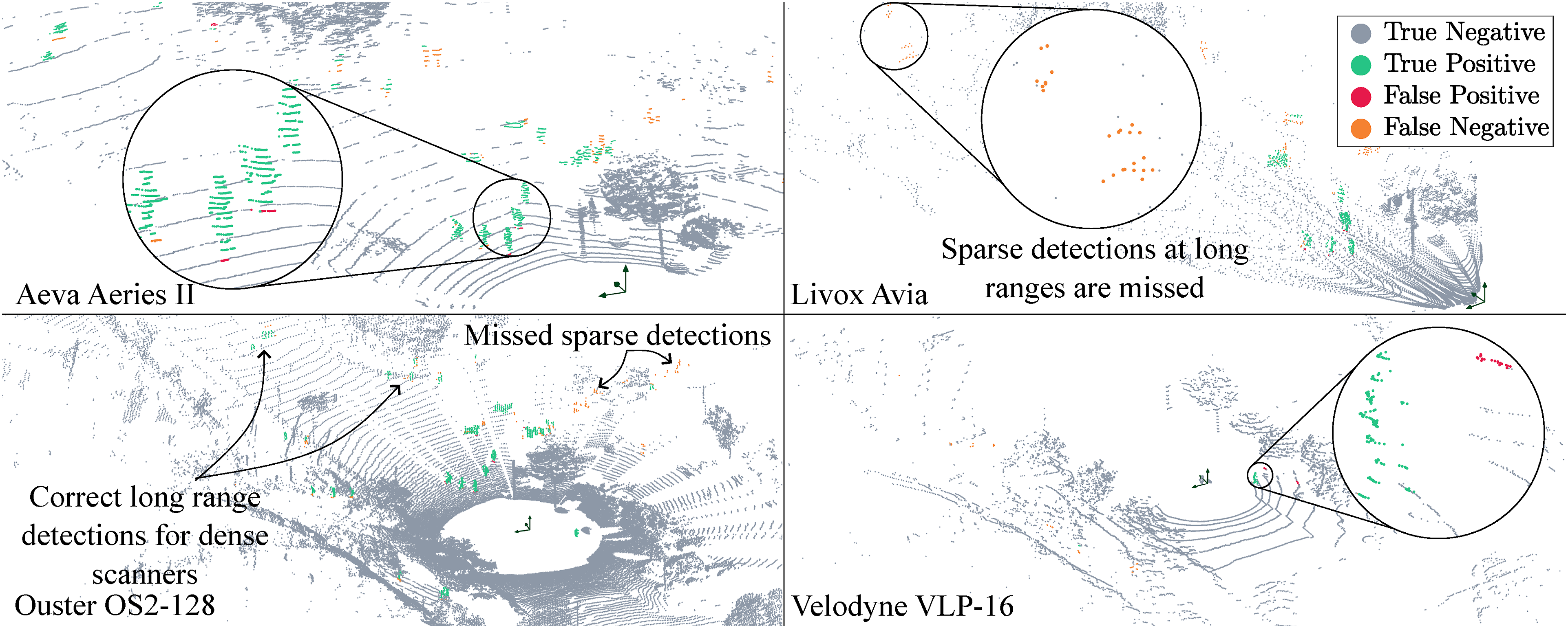

Method	Sequence IoU (%)
	L	A	O	V
4DMOS, online	52.1	54.0	64.2	4.7
MapMOS, scan	58.9	63.2	81.4	4.3
This paper, Δ = 0.20 m	50.7	68.0	73.0	35.8
This paper, Δ = 0.25 m	51.9	69.0	74.2	36.1
4DMOS, delayed	59.0	58.3	70.4	5.4
MapMOS, volume	62.7	66.6	82.9	5.8

We present only the generalized performance of alternative approaches without retraining them on the new dataset, as retraining would undermine our goal of evaluating algorithm robustness in unseen environments and new applications. An interesting study was conducted by the authors of the dataset, who trained 4DMOS and MapMOS with various combinations of the sensor data to examine the impact on performance. They acknowledge the significant improvements required for existing MOS methods to operate in a sensor-agnostic approach, providing further motivation for this work. Dynablox constructs a global TSDF map using the point cloud data and hence requires significant computational memory to be evaluated on the HeLiMOS dataset. We evaluate a fraction of the dataset and qualitatively analyze its performance compared to the proposed approach in Figure 7. Dynablox performs well with dense point cloud data in the Ouster sequence, but has missed and incomplete detections for the other sensors, which record lower-density point clouds. The sensor-specific configuration parameters were updated where appropriate, or else configured to provide the best result possible. The proposed approach provides better detection for all sensors.

Figure 7.

A comparison between the performance of Dynablox and the proposed approach for all sequences using their default configurations. Dynablox performs well with high-density point clouds in the Ouster sequence. However, low-density scan patterns in the other sequences result in incomplete detections. The figure is best viewed in colour.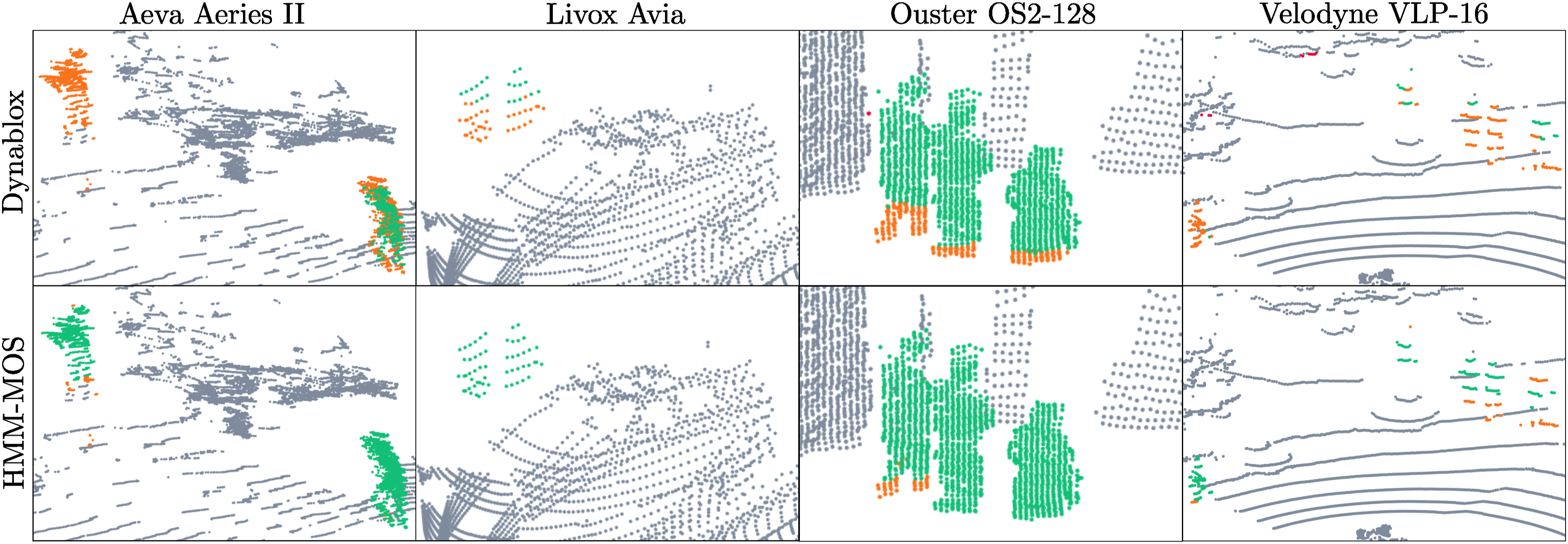

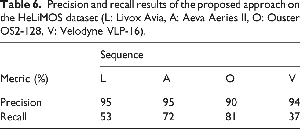
Examining the average precision and recall in Table 6 indicates the performance is precise, with the main limitation in capturing the entire object.

Table 6.

Precision and recall results of the proposed approach on the HeLiMOS dataset (L: Livox Avia, A: Aeva Aeries II, O: Ouster OS2-128, V: Velodyne VLP-16).

Metric (%)	Sequence
	L	A	O	V
Precision	95	95	90	94
Recall	53	72	81	37

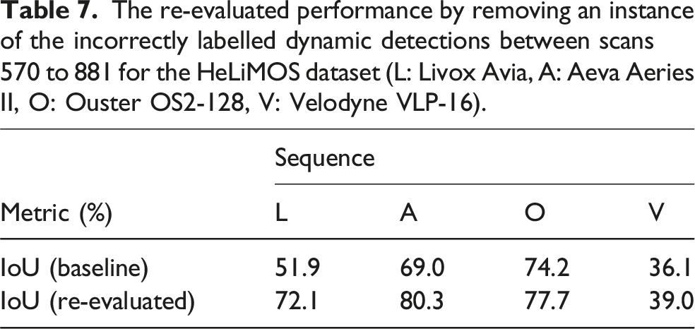
It is important to mention that the ground-truth labels any dynamic objects that have moved throughout the sequence. This includes objects that transition from being dynamic to static and objects that transition from being static to dynamic. These situations occur in several scenes, drastically reducing the recall. The effect is detrimental to the Livox (L) results for all methods. The ground-truth labels are useful for map cleaning approaches (e.g. Removert, ERASOR), but they hinder the performance of all MOS approaches as the vehicles transition from stationary to moving. The proposed approach cannot predict if an object will move and capture these instances. Results on all LiDARs confidently detect moving objects only. Figure 8 depicts this scenario, and Table 7 quantifies the significant increase in the re-evaluated performance when scans 570–881 are correctly labelled. The Livox (L) and Aeva (A) sequences are significantly affected by the incorrectly labelled static vehicles due to their mounting locations and field of view. The Velodyne (V) sensor’s field of view is blocked at its mounting location, resulting in a minor performance change. While the Ouster (O) sequence is affected, the relative number of false positives in this sequence is outweighed by the true positive detections captured by its 360-degree FOV. For comparison, the Ouster sequence is labelled with approximately 8.4e6 dynamic measurements, whereas the Livox sequence has 1.8e6 dynamic measurements only.

Figure 8.

A snapshot of the environment in scans 570-881 from the HeLiMOS dataset. Vehicles are labelled as dynamic but move in a future instance. This scenario incorrectly depicts the recall metrics of the Aeva, Livox, and Ouster sequences for all MOS methods. The Velodyne has a limited view of these vehicles due to its mounting position. The figure is best viewed in colour.

Table 7.

The re-evaluated performance by removing an instance of the incorrectly labelled dynamic detections between scans 570 to 881 for the HeLiMOS dataset (L: Livox Avia, A: Aeva Aeries II, O: Ouster OS2-128, V: Velodyne VLP-16).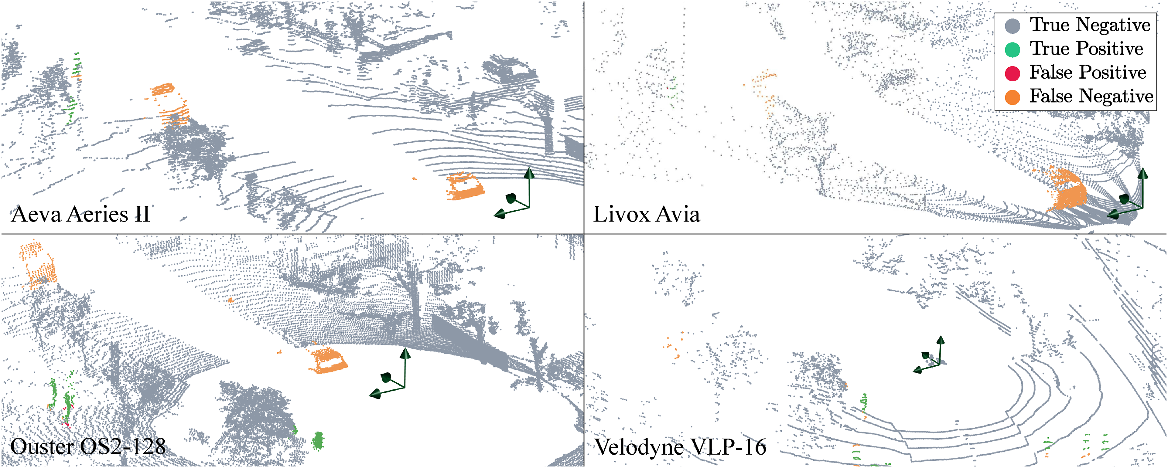

Metric (%)	Sequence
	L	A	O	V
IoU (baseline)	51.9	69.0	74.2	36.1
IoU (re-evaluated)	72.1	80.3	77.7	39.0

The results for the Velodyne sensor (V) show the most significant performance discrepancy in comparison to the other LiDARs for all methods. The 16-beam scans provide challenging input, as it is difficult to discriminate between noisy detections and sparse measurements at long ranges. Figure 6 illustrates the drastic difference in scan density for all LiDARs. The proposed approach demonstrates consistent performance across all scenarios, independent of the sensor characteristics, as it uses information about free and occupied space from the point cloud data only. This is seen as an advantage of our proposed approach.

Table 8 displays a comparison of the average processing frame rate. The algorithm provides real-time results for all sensors except the Ouster due to its high-density scans. 4DMOS and MapMOS provide 10 Hz results for full-range scans but are GPU-based. The proposed algorithm uses CPU threading only.

Table 8.

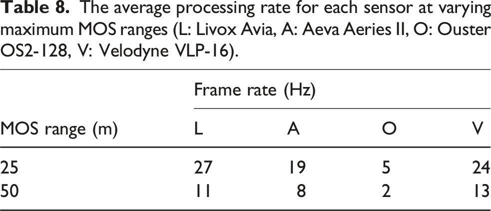
The average processing rate for each sensor at varying maximum MOS ranges (L: Livox Avia, A: Aeva Aeries II, O: Ouster OS2-128, V: Velodyne VLP-16).

MOS range (m)	Frame rate (Hz)
	L	A	O	V
25	27	19	5	24
50	11	8	2	13

Apollo-Southbay

The Apollo-Southbay dataset by Lu et al. (2019) is commonly used to evaluate the generalization of learning-based approaches outside their training on the Semantic Kitti dataset. Though both datasets use Velodyne HDL-64 LiDARs, they are mounted on different vehicles at different heights relative to the ground. Table 9 displays the results of the proposed approach in comparison to existing methods benchmarked by Mersch et al. (2023). The proposed approach outperforms the online and delayed variants of 4DMOS and is second to MapMOS.

Table 9.

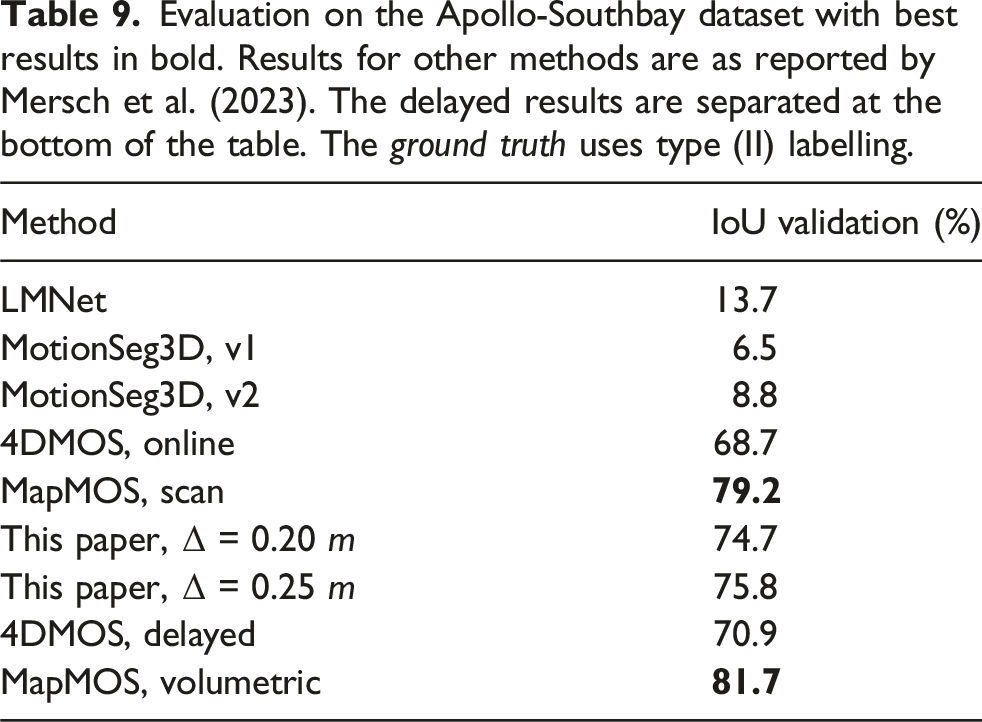
Evaluation on the Apollo-Southbay dataset with best results in bold. Results for other methods are as reported by Mersch et al. (2023). The delayed results are separated at the bottom of the table. The ground truth uses type (II) labelling.

Method	IoU validation (%)
LMNet	13.7
MotionSeg3D, v1	6.5
MotionSeg3D, v2	8.8
4DMOS, online	68.7
MapMOS, scan	79.2
This paper, Δ = 0.20 m	74.7
This paper, Δ = 0.25 m	75.8
4DMOS, delayed	70.9
MapMOS, volumetric	81.7

The proposed approach accurately identifies moving vehicles, cyclists, and pedestrians without any parameter tuning and identifies minimal false positives as displayed in Figure 9 (left). Like the HeLiMOS dataset, AutoMOS’s ground-truth labels (Chen et al., 2022) classify objects as dynamic if they moved at any point during the sequence. This classification approach significantly alters recall scores when vehicles stop moving.

Figure 9.

The proposed approach accurately identifies objects of various sizes travelling at different speeds indicated by the green measurements. False positives shown in red arise at the boundary of the static and dynamic points, such as where the wheels touch the ground. The scan on the right shows a vehicle labelled as dynamic by the ground truth that transitioned from being dynamic to static. These instances incorrectly portray algorithm performance. The figure is best viewed in colour.

There is a sequence of 150 scans in Apollo sequence 00 where a vehicle transitions from being dynamic to static behind the instrumented vehicle. The ground truth continues to label these as measurements corresponding to a dynamic object. Figure 9 (right) shows an example of this situation. Correcting the ground truth by ignoring these measurements results in a 17% increase in recall. Furthermore, removing all such instances between scans 180–530 results in a 26% increase in recall. This represents a significant discrepancy when benchmarking results are compared to other methods that continue to label these measurements as dynamic.

We firmly maintain that a moving object should be defined as one that is actively in motion during the current scan, not one that moved previously or might move later. Our approach adheres to this definition by correctly identifying temporarily stationary vehicles as static, while the ground truth continues to label them as dynamic based on their movement history.

The algorithm processes the Velodyne HDL-64 scans at 10 Hz for a 25 m MOS range, and at 5.5 Hz for a 50 m range.

Waymo, KITTI, nuScenes, Avia

M-detector by Wu et al. (2024) benchmarks performance on three open datasets; KITTI (Geiger et al., 2012), Waymo (Sun et al., 2020), and nuScenes (Fong et al., 2022). Wu et al. (2024) provide the ground truth pointwise labels for these datasets. The KITTI dataset is labelled using the bounding boxes provided in the object-tracking sequences. The velocity of the bounding boxes is estimated using consecutive frames, with all measurements in bounding boxes having a velocity greater than a threshold, labelled as dynamic, 0.5 m/s for pedestrians and 1.0 m/s for vehicles. The authors of this paper label any dynamic detections as moving. In comparison to the other experiments in this paper, this introduces a different evaluation metric. A similar approach is used for the Waymo and nuScenes datasets. The method proposed in our work captures any moving objects, irrespective of their speed. This introduces an inaccuracy when benchmarking results. It must be noted that the KITTI ground-truth labels only capture moving objects within a 120-degree field of view due to the limited object-tracking bounding boxes. Any motion behind the sensor or on the sides is not captured. Wu et al. (2024) additionally record and label a unique indoor dataset capturing small flying objects with a Livox Avia. This dataset challenges learning-based approaches as the scan pattern, object shape, and dynamics are very different from the training data.

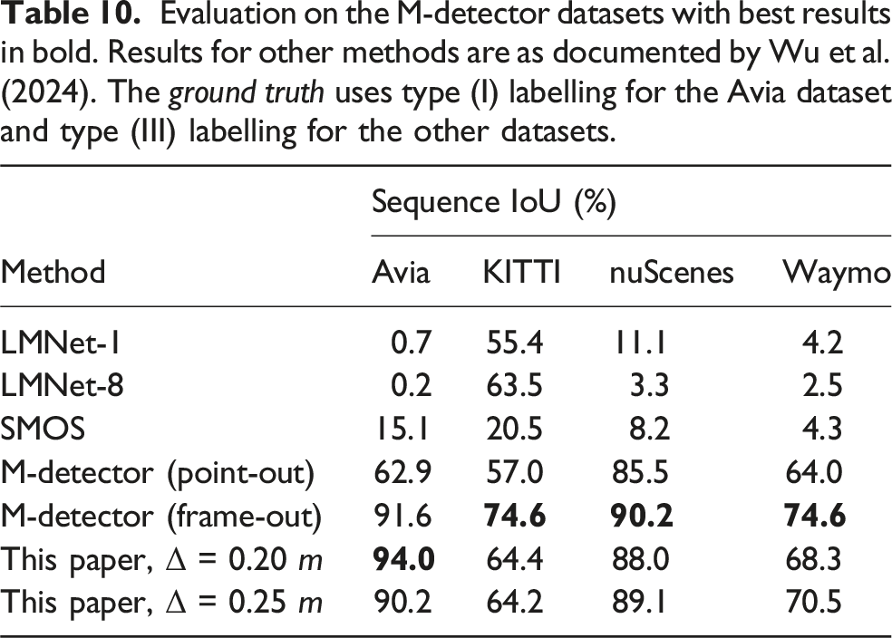
Figure 10 illustrates sample detections from the various datasets. The proposed approach successfully captures dynamic objects in all tests. The nuScenes dataset captures a large number of points on the vehicle itself. The sequence of Avia scans shows a small, fast-moving object correctly captured by the proposed algorithm. The example for the Waymo dataset illustrates an instance of the minimum velocity threshold, labelling the vehicle as slowing down as a static object ( $<1$  m/s). Relabelling scans 28 to 97 in sequence 16 results in a 7% increase in precision and a 4% increase in the sequence’s IoU. This is a significant increase, given the minor differences in the benchmarking comparison. Furthermore, evaluating MapMOS on the same sequence results in a 13% increase in precision when using its definition of a moving point.

Figure 10.

Example results on the datasets benchmarked by M-detector. The Waymo dataset uses a 64-beam custom LiDAR. The proposed approach correctly identifies moving objects. False positives occur (i) at the boundary of static and dynamic points, and (ii) due to the minimum velocity threshold on the dynamic objects. The nuScenes dataset uses a 32-beam LiDAR. A large density of points is captured on the vehicle itself, biasing the results. The Avia dataset tests the capability to capture small and fast-moving objects, providing a unique experimental study. The figure is best viewed in colour.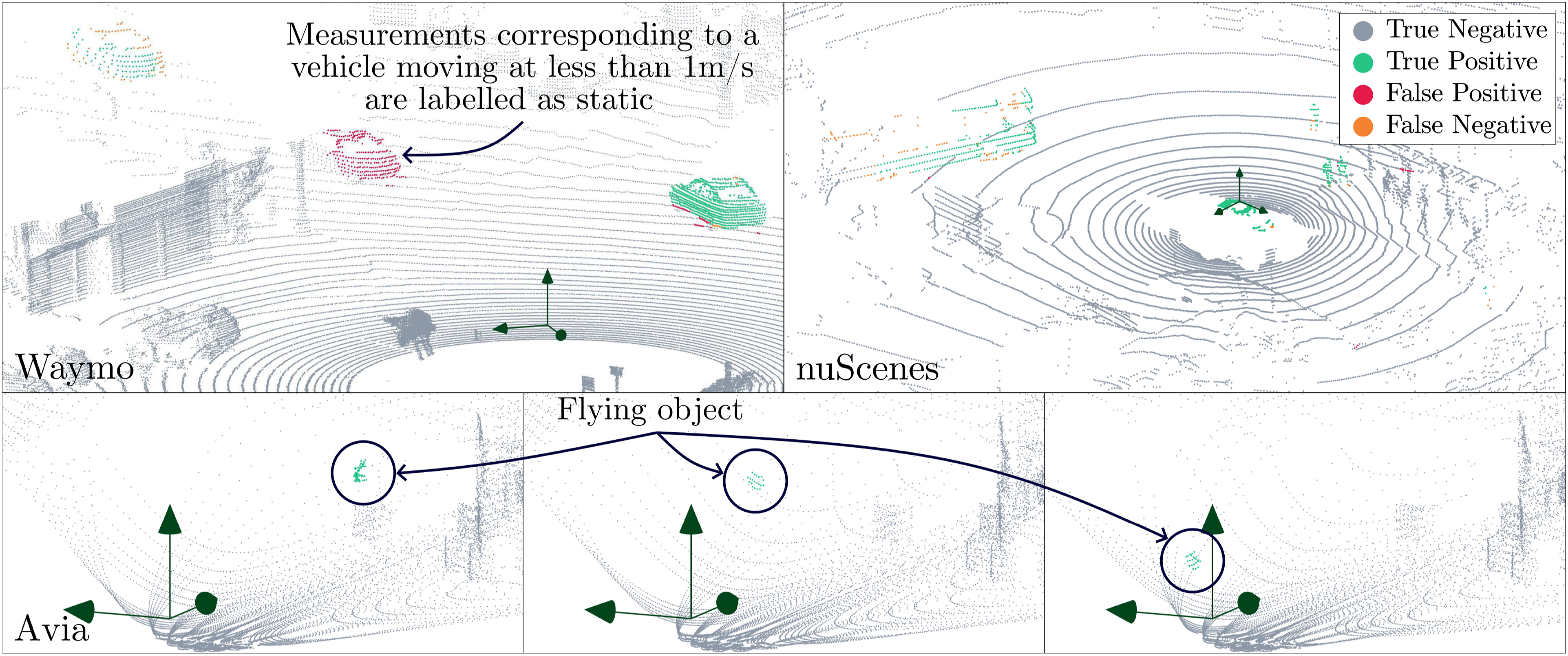

Table 10 displays the performance of the proposed approach on the datasets and in comparison to M-detector. The proposed algorithm performs consistently in all datasets, performing on par with M-detector and outperforming the learning-based approaches. We acknowledge the difference in the ground-truth labelling process with the minimum velocity thresholds. The proposed algorithm uses the same configuration for all sensors in all experiments used in the other datasets. M-detector configures a set of 14 parameters for each sensor, with different parameters for the depth map generation, occlusion check, event detection, and map consistency. The finer tuning helps achieve better results.

Table 10.

Evaluation on the M-detector datasets with best results in bold. Results for other methods are as documented by Wu et al. (2024). The ground truth uses type (I) labelling for the Avia dataset and type (III) labelling for the other datasets.

Method	Sequence IoU (%)
	Avia	KITTI	nuScenes	Waymo
LMNet-1	0.7	55.4	11.1	4.2
LMNet-8	0.2	63.5	3.3	2.5
SMOS	15.1	20.5	8.2	4.3
M-detector (point-out)	62.9	57.0	85.5	64.0
M-detector (frame-out)	91.6	74.6	90.2	74.6
This paper, Δ = 0.20 m	94.0	64.4	88.0	68.3
This paper, Δ = 0.25 m	90.2	64.2	89.1	70.5

Table 11 shows the average processing rates for the proposed algorithm at varying MOS ranges, compared to the results published by M-detector. A similar trend is observed with previous datasets where low-density scanners are processed significantly faster. The Avia dataset is recorded indoors.

Table 11.

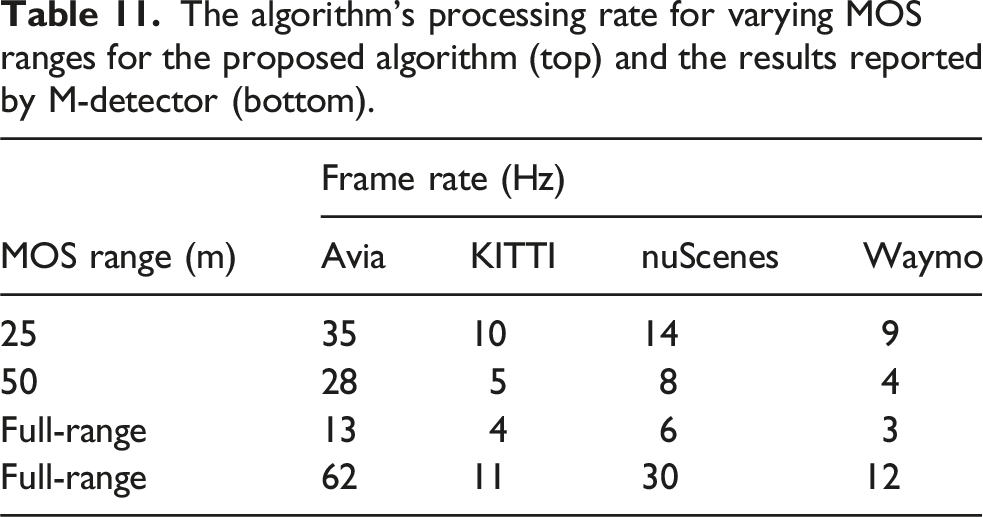
The algorithm’s processing rate for varying MOS ranges for the proposed algorithm (top) and the results reported by M-detector (bottom).

MOS range (m)	Frame rate (Hz)
	Avia	KITTI	nuScenes	Waymo
25	35	10	14	9
50	28	5	8	4
Full-range	13	4	6	3
Full-range	62	11	30	12

DOALS

The DOALS dataset by Pfreundschuh et al. (2021) consists of eight sequences at four locations recorded using a handheld OS1-64 LiDAR at 10 Hz. The sequences are recorded in indoor and outdoor human-centric environments. We use SiMpLE (Bhandari et al., 2024) to estimate the sensor pose accurately and use the deskewed point clouds. Deskewing plays a significant role in correcting the jittery LiDAR motion from the handheld sensor. Schmid et al. (2023) label 10 scans per sequence that do not specifically discriminate between moving and non-moving objects, with all pedestrian-looking points labelled as dynamic. This eliminates the ambiguity in the different definitions of moving points, but also means a perfect IoU cannot be achieved. In line with the evaluation process by Schmid et al. (2023), the IoU is computed for all 10 labelled scans per sequence, with the mean value displayed in Table 12. Table 13 shows the mean processing frame rate for all sequences. The Station sequence (ST) has the slowest processing time due to its large open recording environment, which requires updating a significant number of free voxels.

Table 12.

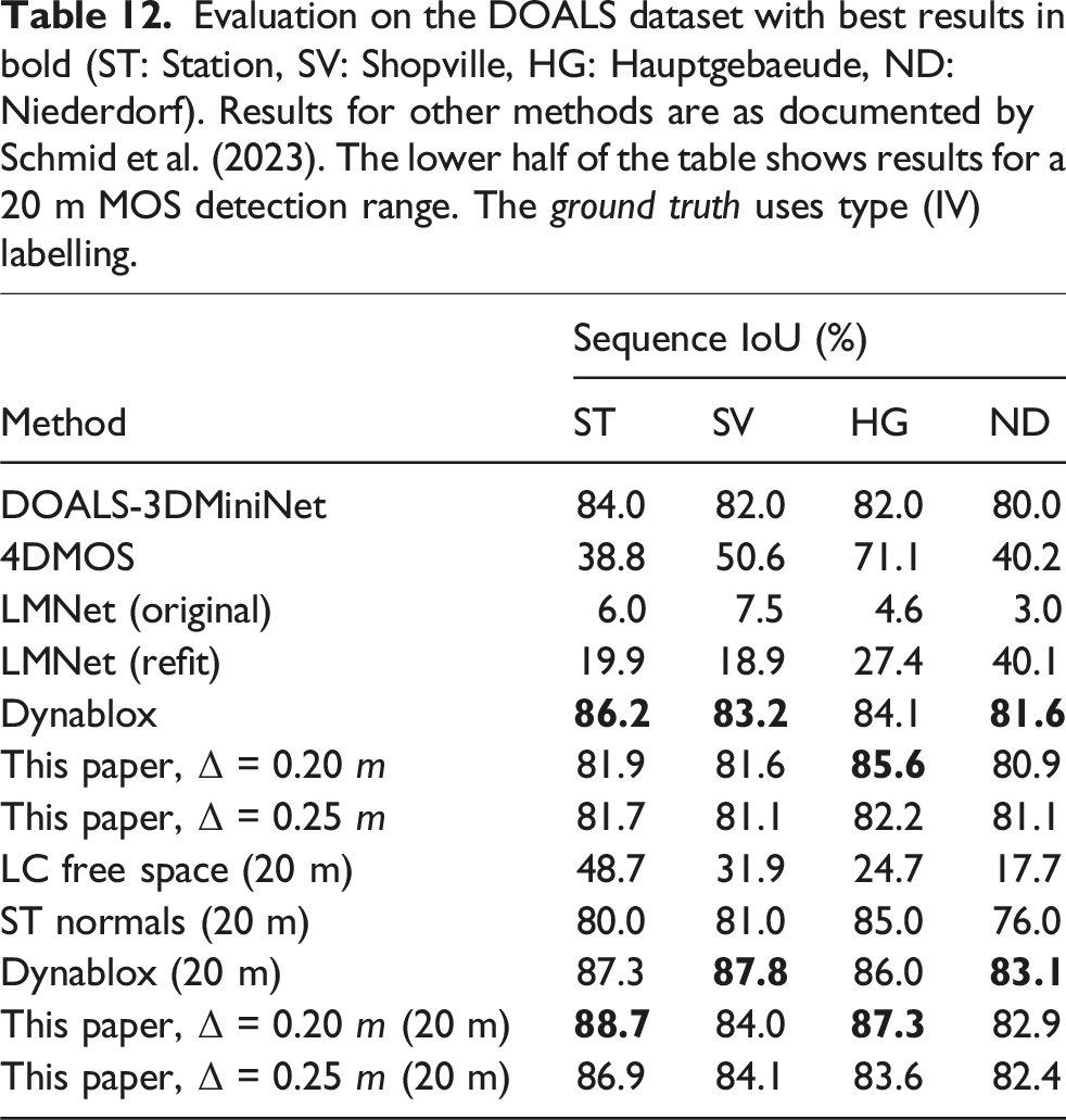
Evaluation on the DOALS dataset with best results in bold (ST: Station, SV: Shopville, HG: Hauptgebaeude, ND: Niederdorf). Results for other methods are as documented by Schmid et al. (2023). The lower half of the table shows results for a 20 m MOS detection range. The ground truth uses type (IV) labelling.

Method	Sequence IoU (%)
	ST	SV	HG	ND
DOALS-3DMiniNet	84.0	82.0	82.0	80.0
4DMOS	38.8	50.6	71.1	40.2
LMNet (original)	6.0	7.5	4.6	3.0
LMNet (refit)	19.9	18.9	27.4	40.1
Dynablox	86.2	83.2	84.1	81.6
This paper, Δ = 0.20 m	81.9	81.6	85.6	80.9
This paper, Δ = 0.25 m	81.7	81.1	82.2	81.1
LC free space (20 m)	48.7	31.9	24.7	17.7
ST normals (20 m)	80.0	81.0	85.0	76.0
Dynablox (20 m)	87.3	87.8	86.0	83.1
This paper, Δ = 0.20 m (20 m)	88.7	84.0	87.3	82.9
This paper, Δ = 0.25 m (20 m)	86.9	84.1	83.6	82.4

Table 13.

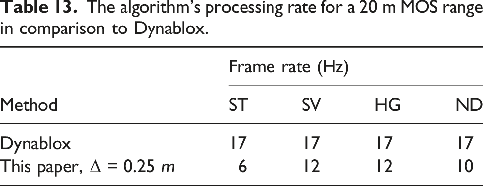
The algorithm’s processing rate for a 20 m MOS range in comparison to Dynablox.

Method	Frame rate (Hz)
	ST	SV	HG	ND
Dynablox	17	17	17	17
This paper, Δ = 0.25 m	6	12	12	10

Results are provided for full-range (172 m) and short-range (20 m) test cases. We outperform existing learning-based approaches such as LMNet and 4DMOS and are on par with Dynablox for the full-range tests. The learning-based approaches fail to generalize performance as indicated by the low IoU. We outperform all approaches on the short-range test with similar results to Dynablox again. We achieve a mean precision of 96% and recall of 90% for all evaluated scans. The high precision indicates the low false positives, whereas the slightly lower recall highlights the challenge of capturing the entire object, but is also affected by the labelling process.

Sipailou campus

The Sipailou campus dataset by Zhou et al. (2023) consists of eight sequences recorded by a Livox Avia LiDAR mounted to an unmanned ground vehicle traversing the Southeast University Sipailou Campus. The LiDAR has a non-repetitive scanning pattern and a different field of view, providing a unique dataset to test the generalization capabilities of MOS methods. The provided sensor poses are used. Using the same configuration as other tests, we outperform all approaches as displayed in Table 14.

Table 14.

Evaluation on the Sipailou Campus dataset with best results in bold. Results for other methods are as reported by Zhou et al. (2023). The ground truth uses type (I) labelling.

Method	IoU (%)
	Validation	Test
LMNet	5.4	6.9
MotionSeg3D	6.8	6.7
4DMOS	78.5	82.3
Motion-BEV	50.4	52.0
Motion-BEV-h	70.9	71.5
This paper, Δ = 0.25 m	84.9	86.0
This paper, Δ = 0.20 m	84.8	86.1

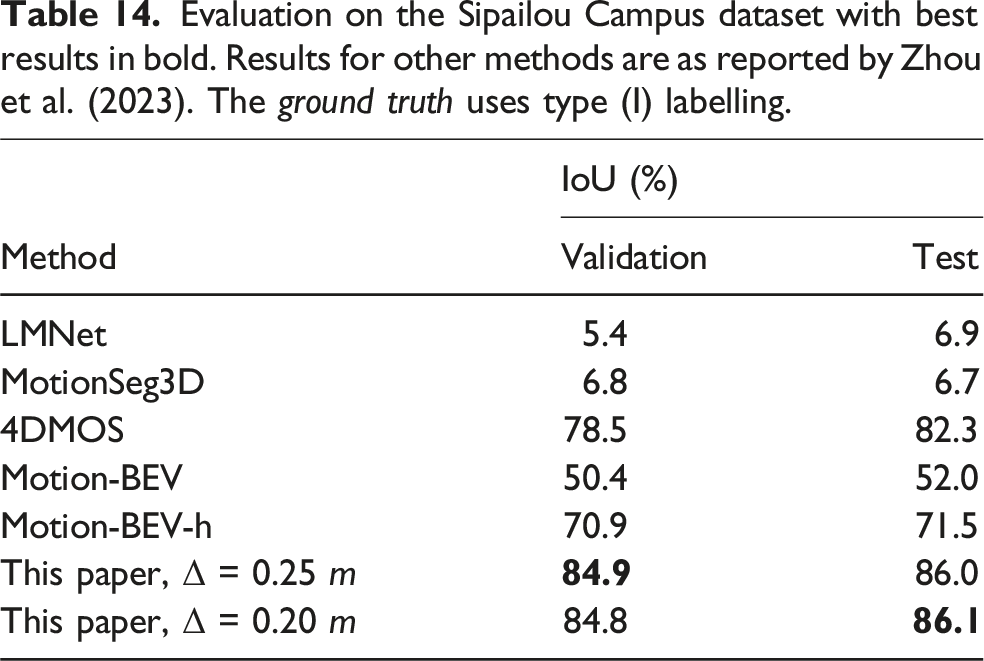
The results for the other methods are used directly from Zhou et al. (2023) and only consider the evaluation without retraining the networks on the new data to provide a fair test of generalized performance. The results are evaluated using the Semantic KITTI API (Behley et al., 2019) to be consistent with the original evaluation process and benchmark results. Learning-based approaches such as LMNet, MotionSeg3D, and MotionBEV fail to generalize due to differences in the sensor’s characteristics. 4DMOS demonstrates strong generalization with its unique design of learning changes in sequential data, being model-independent. The proposed approach cannot capture sparse measurements at longer ranges corresponding to dynamic objects, as they are difficult to differentiate from noisy estimates. The results are processed with an average frame rate of 10 Hz for a maximum 50 m MOS range.

Case study: Detecting moving objects in an excavator’s workspace

This Section investigates the use of MOS in detecting dynamic objects within an excavator’s workspace using onboard LiDAR. Excavator operators have limited visibility from the cab, and their proximity to other machines can result in collisions, leading to operator fatalities, equipment damage, and significant operational downtime. Sensors such as LiDAR enable imaging of the workspace’s immediate environment, and extending the discussed MOS algorithms to this scenario provides the ability to identify the presence of dynamic objects in the agent’s workspace.

This case study demonstrates the performance of the proposed algorithm in detecting the presence of dynamic objects within the excavator’s workspace. The sensor data is from a field study where two Velodyne HDL-64 LiDARs were mounted on the back of an excavator. Two scenarios from the dataset are presented: (i) identifying the presence of a light vehicle that enters the work area during a shift change, and (ii) the changes in the workspace during regular operation as haul trucks come and go.

Figure 11(a) shows the field environment, displaying the instrumented excavator and haul trucks moving in its workspace. Detection results for the left sensor are shown as the excavator is loading trucks to its left only.

Figure 11.

(a) A view of the case study’s field environment. Two LiDARs are mounted to the rear of the house to image the workspace. Trucks enter and leave the workspace as they are loaded. (b) A comparison of scans captured from the Semantic KITTI dataset (left) and the excavator (right). The change in sensor orientation, mounting height, motion profile, and scanning frequency, pose challenges to providing accurate MOS predictions in an unknown environment for learning-based approaches.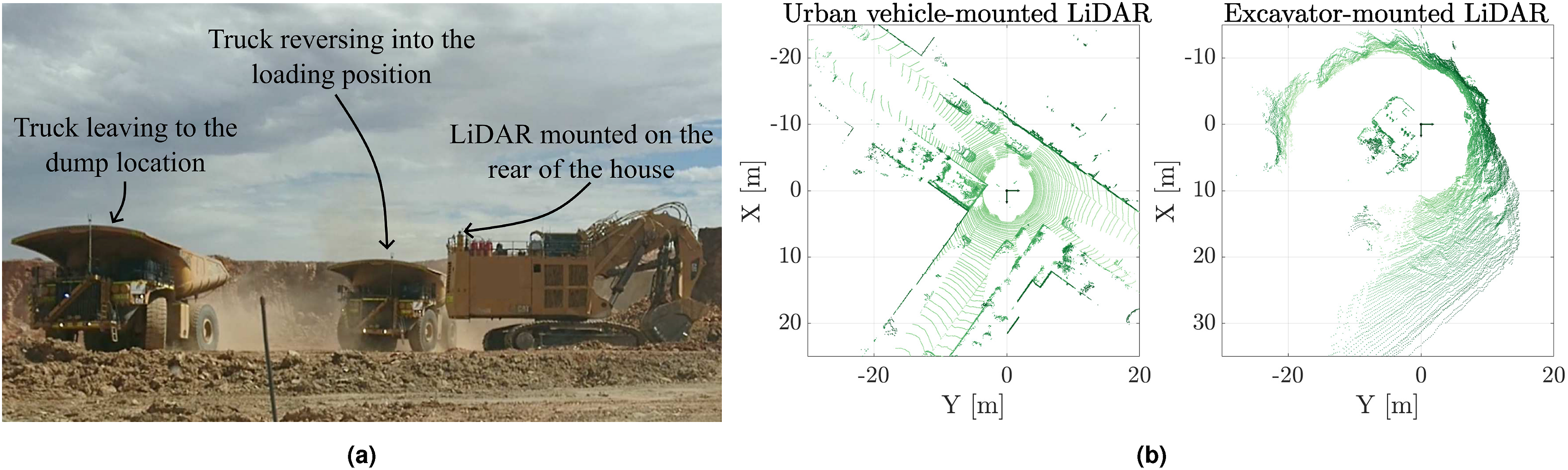

The performance of the proposed algorithm is compared to 4DMOS (Mersch et al., 2022) and MapMOS (Mersch et al., 2023), both of which were trained on the Semantic KITTI dataset (Behley et al., 2019), and Dynablox (Schmid et al., 2023). The Semantic KITTI dataset and this case study both use the Velodyne HDL-64 sensor. However, the sensor’s motion profile, scanning frequency, mounting height, and mounting orientation are drastically different in both datasets. Figure 11(b) displays examples of scans from the Semantic KITTI dataset (left) and the excavator (right). The scan from the Semantic KITTI dataset provides high coverage of the workspace at all times. In contrast, the scan from the excavator is unstructured and has a limited view of different areas in the workspace as the machine slews on its swing axis. The proposed algorithm continues to perform well; 4DMOMS and MapMOS are less effective. Dynablox also performs well, with the high-density scans matching the sensor characteristics from its published evaluation.

All MOS approaches use the same inputs for fair testing, with Dynablox, 4DMOS, and MapMOS configured using their default parameters. The sensor’s pose is estimated using the point cloud data. All detections are performed in the sensor’s frame, allowing for testing with the open-source repositories.

The first scenario assesses the ability of the MOS approaches to identify a light vehicle and its operator within the excavator’s workspace during a shift change. Figure 12 displays the dynamic detection results for the MOS approaches on a sequence of scans as a light vehicle enters the excavator’s workspace. MapMOS and the proposed algorithm yield nearly identical results for all scans, completely capturing the moving vehicle. Dynablox performs well, only missing a small fraction of the vehicle’s bonnet in the last frame. 4DMOS provides a late partial detection, possibly due to the receding horizon used to fuse beliefs about dynamic measurements. This scenario provided a simple scenario with a well-observed vehicle, being similar to the dynamic detections in the Semantic KITTI dataset.

Figure 12.

A sequence of scans showing a light vehicle entering the excavator’s workspace during an operator shift change. The estimated dynamic detections are shown in green, with missed detection coloured orange. 4DMOS provides late detection and only partially labels the vehicle. The proposed approach, MapMOS, and Dynablox provide fast and accurate detection of the vehicle for the entire sequence. The figure is best viewed in colour.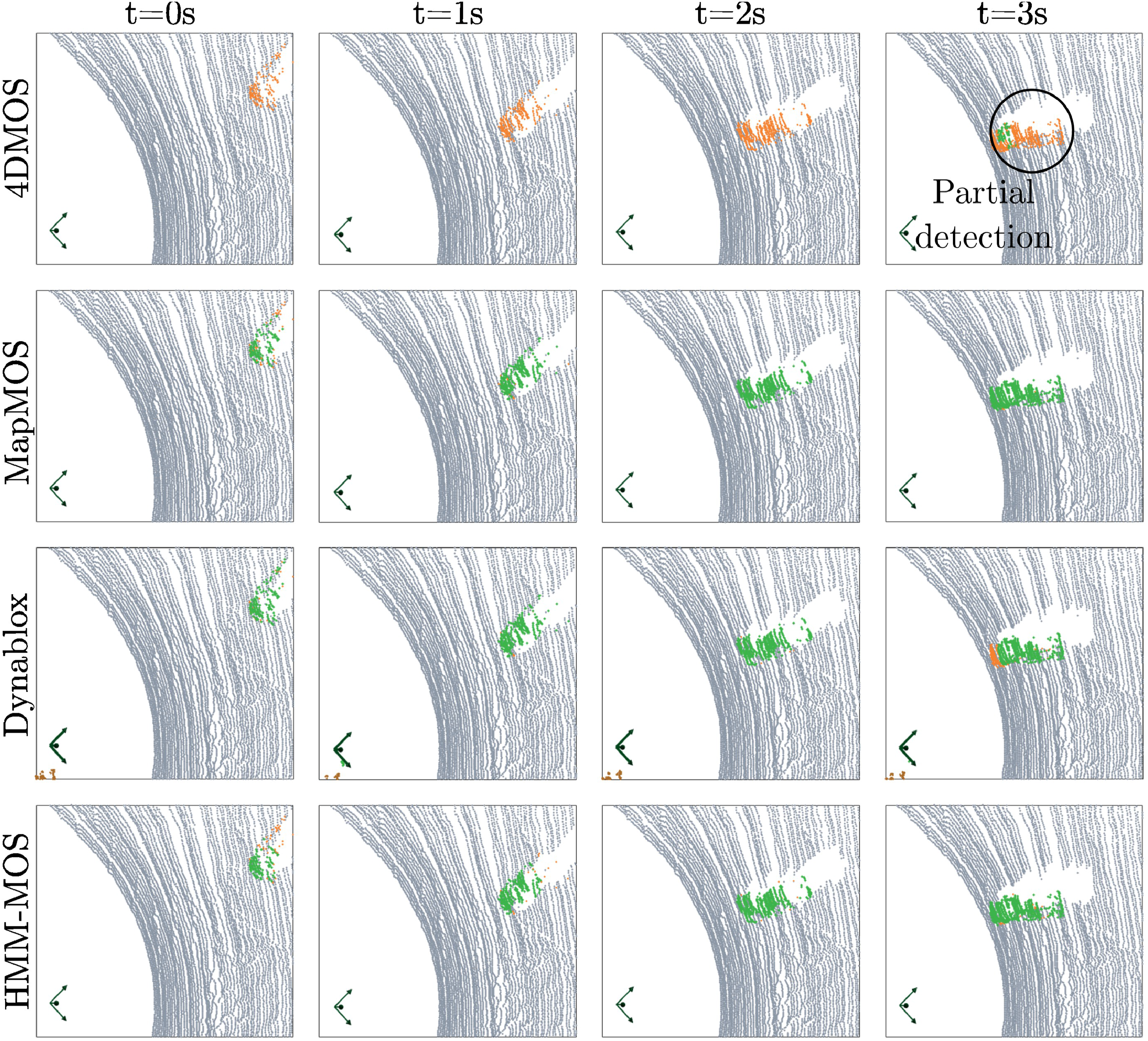

The second scenario involves a truck maneuvering into the loading position. Figure 13 displays the performance of the MOS approaches for a sequence of scans during the scenario. 4DMOS detects the moving truck in most frames, but generates numerous false positives on the terrain, failing to identify the truck accurately. MapMOS captures the truck in the first frame, provides a partial detection for the second frame, but fails to capture any detections thereafter. The proposed algorithm and Dynablox provide consistent detection across all frames, regardless of the truck’s observability.

Figure 13.

A sequence of scans of a truck maneuvering into the loading position. The estimated dynamic detections are shown in green, incorrect detections in red, and missed detection coloured orange. Only the proposed approach and Dynablox correctly identify all detections, regardless of the moving truck’s observability. MapMOS correctly identifies the truck when it is fully observable, but misses all occasions of partial visibility in frames. The figure is best viewed in colour.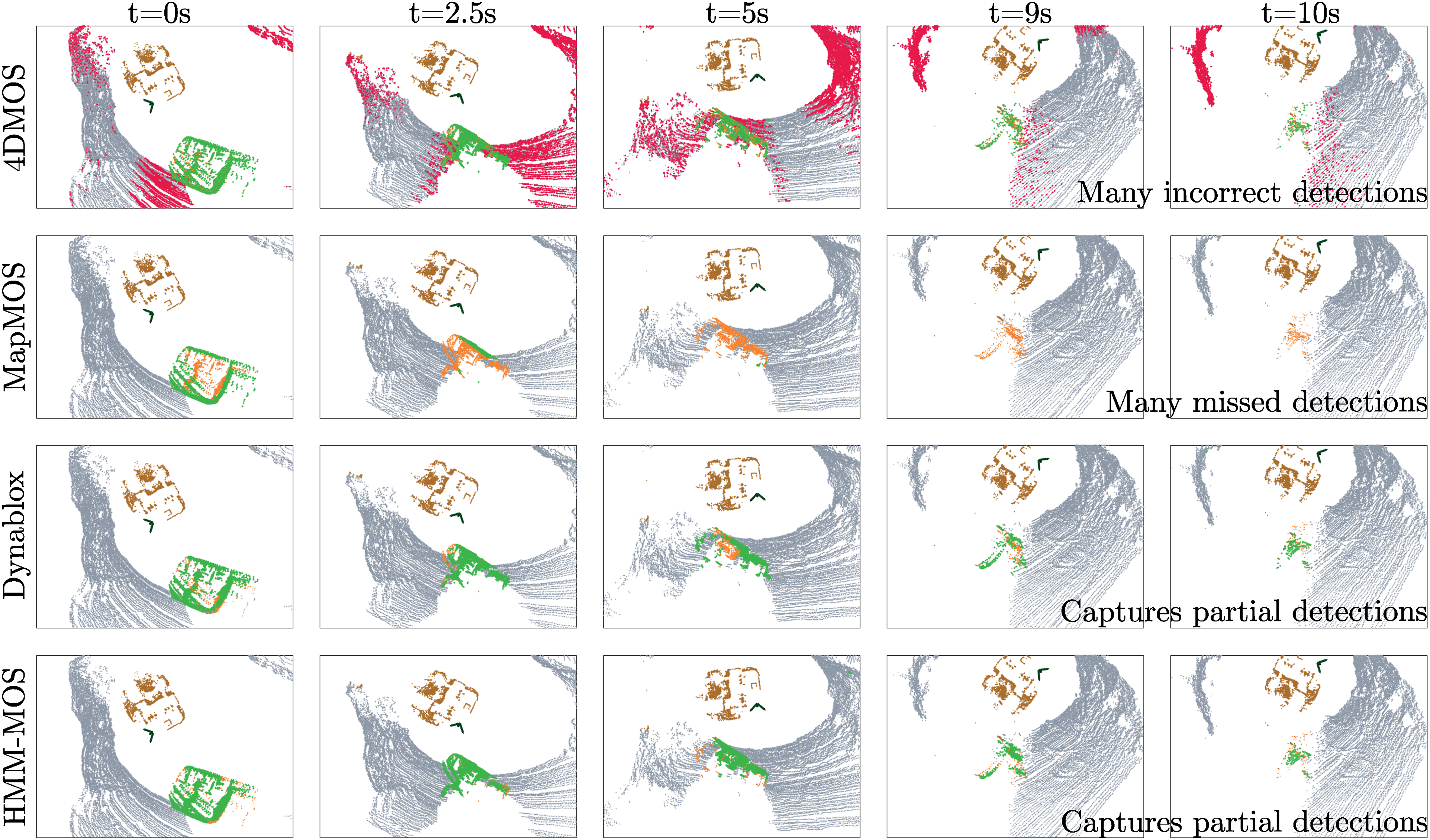

Both scenarios provide unique scenarios for examining the performance of the MOS approaches. MapMOS performs well without being retrained, but is unable to capture dynamic measurements in partially observable conditions. Its strength lies in using the probabilistic backend to keep a history of the occupied and free space. 4DMOS fails as the scene’s observability changes throughout its receding horizon, from which the dynamic detections are estimated. Dynablox performs well with its default configuration with only minor missed detections. The dense point cloud data closely matches the DOALS dataset used to originally evaluate Dynablox’s performance. The proposed algorithm provides consistent performance in both scenarios.

Computation

Figure 14(a) displays the mean execution time per scan at varying measurement ranges for different sequences. The proposed algorithm provides real-time results for dynamic object detection within a 20 m sensor range, with computation time increasing at larger ranges. The computation time is bi-proportional to the point cloud’s size and discretization resolution. Using a smaller voxel size increases accuracy, but consequently leads to a larger computation time due to the larger number of voxels that need to be updated. The Sipailou campus dataset and HeLiMOS Velodyne (V) are the fastest due to their small point cloud size in comparison to the high-density Ouster (O) scanners. It is important to note that the 20 m range constraint is applied to the measurement’s ray to allow for accurate modelling of free space. Consequently, this means that modelling large open spaces as in DOALS Station (ST) sequences leads to a slightly longer execution time of 148 ms/scan, compared to the Shopville (SV) sequences with an execution time of 60 ms/scan.

Figure 14.

(a) The algorithm’s timeliness at varying measurement integration ranges for different tests. The algorithm provides real-time results for up to a 20 m range for most scenarios, with computation depending on the point cloud density and voxel size. (b) The computational breakdown of each module for various sequences. The map update and dynamic detection modules are computationally expensive for environments with large open spaces. The figure is best viewed in colour.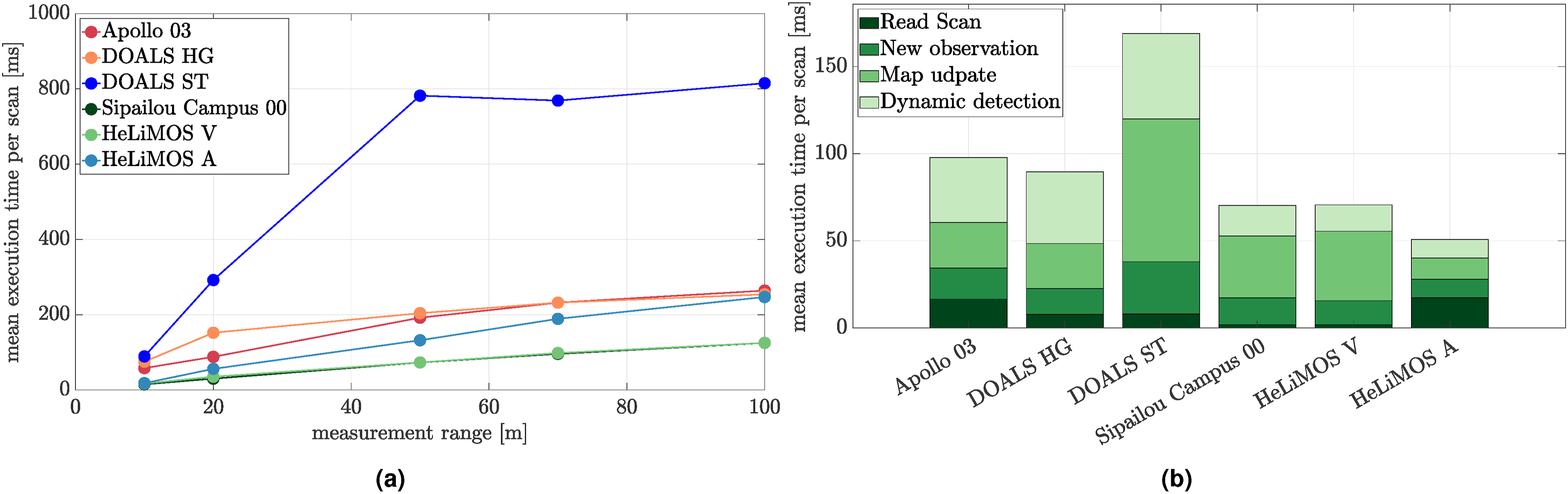

A breakdown of the computational expense of each stage is provided in Figure 14(b). A pattern is observed with the map update and dynamic detection modules being most computationally expensive. Both of these modules involve iterating over all observed voxels. The DOALS ST sequence has a greater computation time for integrating a new observation due to the raycasting operation in a large open space. Implementation of the proposed algorithm relies strongly on CPU threading to provide timely results.

Algorithm configuration

The proposed algorithm has several configuration parameters summarized in Table 1. This Section (i) investigates the effect of the different stages in the MOS pipeline, (ii) provides visualizations of varying configuration parameters to provide a better intuition of their selection, (iii) investigates the sensitivity of the configuration parameters, (iv) details a guide to selecting the configuration parameters, and (v) concludes by analyzing the algorithm’s failure modes.

The purpose of the MOS pipeline’s stages

The proposed algorithm consists of three main stages summarized in Figure 2: integrating a new observation, updating the local map, and detecting dynamic points. In its most straightforward implementation, identifying the changes in the voxel state is sufficient in labelling dynamic points. However, this is inadequate in capturing the entire dynamic object, as articulated objects, such as humans, are not completely dynamic at every instant. Table 15 displays the effect of the algorithm stages on the MOS IoU, precision, and recall for a test sequence from the DOALS dataset. Using a spatial convolution only, the algorithm correctly identifies dynamic objects as highlighted by the high precision but fails to capture the entire object, reflected in the low recall. Adding a temporal aspect significantly increases the recall, leading to a higher IoU. The dilation stage recovers voxels that were disregarded due to the strong constraints on identifying dynamic voxels, leading to a higher recall and consequent increase in IoU. The final preservation stage increases the IoU while slightly decreasing the precision, as false positive detections may be preserved.

Table 15.

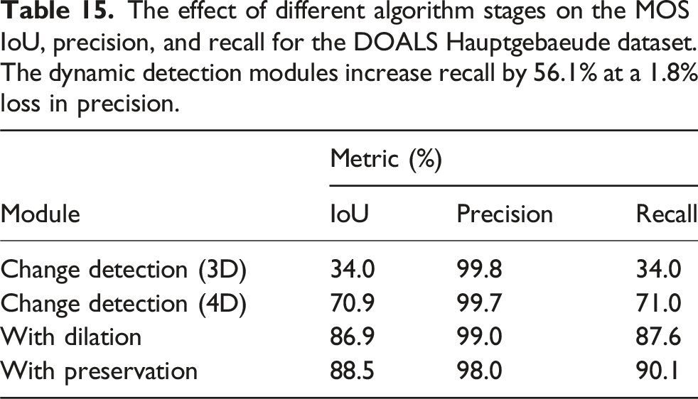
The effect of different algorithm stages on the MOS IoU, precision, and recall for the DOALS Hauptgebaeude dataset. The dynamic detection modules increase recall by 56.1% at a 1.8% loss in precision.

Module	Metric (%)
	IoU	Precision	Recall
Change detection (3D)	34.0	99.8	34.0
Change detection (4D)	70.9	99.7	71.0
With dilation	86.9	99.0	87.6
With preservation	88.5	98.0	90.1

Visualizing different algorithm configurations

Figure 15 visualizes the affect of different configuration parameters on the algorithm’s performance. The first sequence of the DOALS Niederdorf sequence is used for the comparison, with the first column showing the performance of the algorithm using default parameters. The results are analyzed below.

Figure 15.

Visualization of different algorithm configurations. The first column shows the performance of the default configuration for various scans in the first DOALS Niederdorf sequence. Poor parameter selection leads to incomplete or erroneous detection. For example, configuring a very low lumped measurement uncertainty (σ _o ) leads to the voxel update behaving like a Markov model, where new observations directly overwrite the voxel’s existing state. This does not accurately account for measurement uncertainty, which motivates the use of a hidden Markov model. A local window size of one results in incomplete object detection, equivalent to performing a 3D convolution only. Some parameters, such as the transition probability, ϵ ∈ [0, 1], demonstrate low sensitivity across a range of values. The figure is best viewed in colour.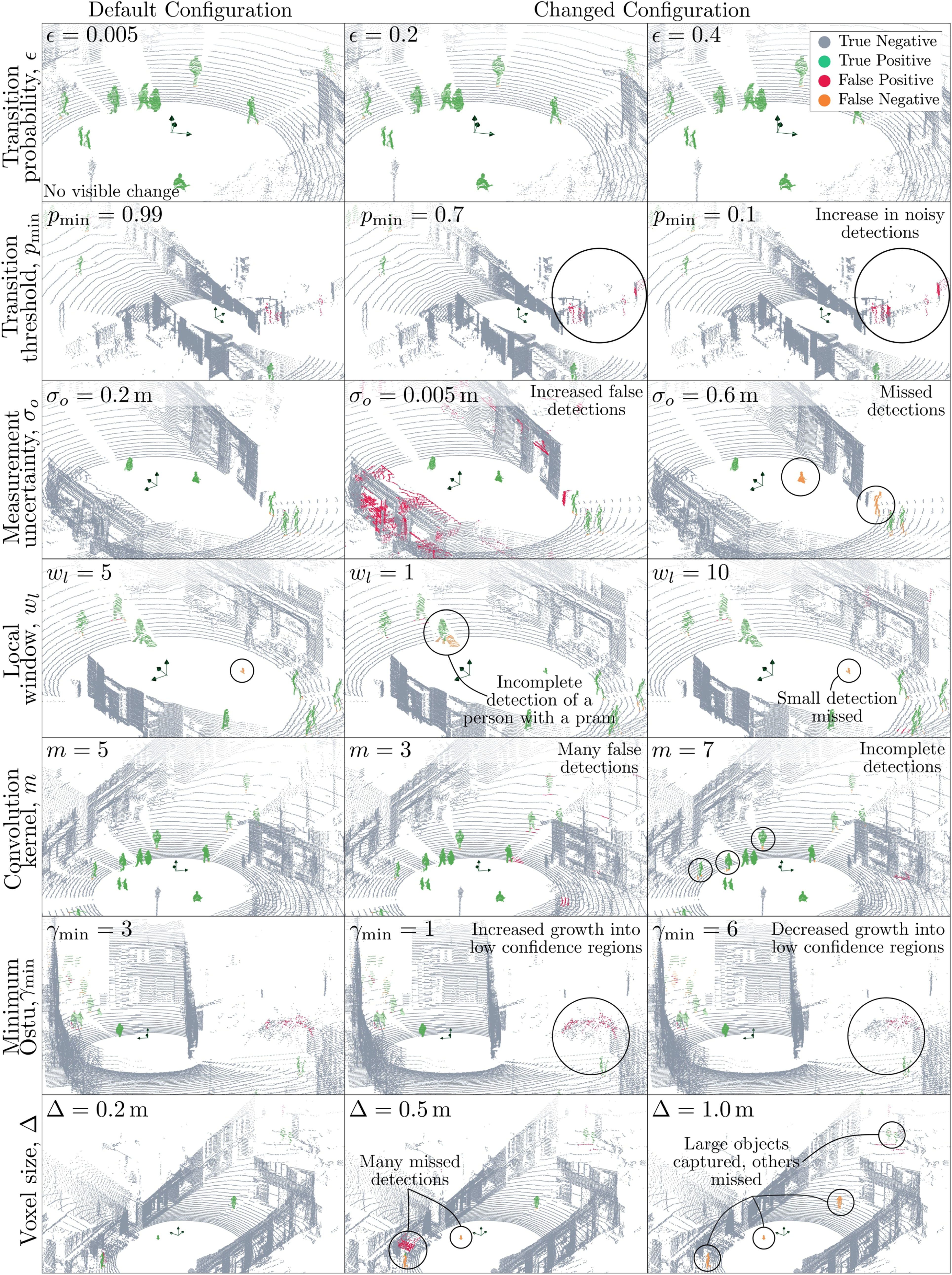

Voxel state update module

A voxel’s transition between states depends on the transition probability (ϵ), the probability threshold for a voxel transitioning state (p_min), and the evidence supporting the transition, computed using σ _o , which is a function of the voxel size (Δ). All these parameters affect a voxel’s state probability.

The state transition matrix, A(ϵ), encodes the transition probabilities between states. Given a new observation, these probabilities are used to model the expected voxel transition and can be tuned to match environment-specific dynamics. We choose to maintain this constant to achieve generalized results across all scenarios. This configuration parameter is insensitive to significant changes, as depicted in the first row in Figure 15. While it does affect the rate at which the transition occurs, the subsequent modules effectively filter false detections.

Decreasing the minimum transition threshold, p_min, results in an increase in the number of noisy detections labelled as dynamic, as shown in the second row. A large value for this threshold is preferred to allow for the sufficient accumulation of evidence to support a transition, minimizing the inclusion of voxels with rapidly changing states.

The uncertainty in the measurements, σ _o , affects the rate at which the state probabilities change. As illustrated in the third row of Figure 15, configuring a very low lumped measurement uncertainty, σ _o , leads to the voxel update behaving like a Markov model, where new observations directly overwrite the voxel’s existing state. This often causes voxels to rapidly switch between free and occupied states, being identified as corresponding to a dynamic object. Thin surfaces, measurements from reflective surfaces such as glass, and the corners of structures are prone to this rapid switching, as illustrated in the results (second row, second column). Assigning a large lumped uncertainty results in a significant delay in identifying dynamic objects, as it slows the change in voxel state probabilities. The result for the larger uncertainty shows multiple missed observations.

The voxel size, Δ, and the lumped uncertainty, σ _o , are strongly linked. The result of the continuous Gaussian function with standard deviation, σ _o , is discretized with a resolution of Δ. The EDF is constructed using voxelized measurements.

Dynamic detection module

The dynamic detection module is configured by the convolution size (m), the lower bound on the minimum Otsu threshold (γ_min), the local window size (w _l ), and the voxel size (Δ). The algorithm computes the likelihood of being dynamic by performing a spatiotemporal convolution over the length of the local window. This likelihood depends on the properties of the dynamic object (size, shape, speed). The kernel attempts to capture the entire object within the local window size, using Otsu’s algorithm to provide a dynamic binary separation threshold between the static and dynamic voxels. The minimum Otsu threshold corresponds to the number of minimum dynamic voxels captured by the kernel across the local window, which is a function of the voxel size, the kernel, and the local window length.

A local window size of one is equivalent to performing a spatial convolution (3D) only, resulting in the incomplete detection of larger objects such as the pram shown in the fourth row in Figure 15. However, it allows for the detection of significantly smaller objects that are usually rejected in the 4D convolution as it is difficult to differentiate from noisy changes in the environment. A larger window size allows for capturing the complete object more effectively.

The size of the convolution kernel, m, is defined in terms of the number of voxels. Consequently, a larger voxel size corresponds to a larger convolution kernel, physically corresponding to the analysis of a larger 3D volume. This additionally requires the minimum Otsu threshold (γ_min) to be revised. For example, a large value for γ_min is only satisfied by a large number of dynamic detections in the convolution kernel across the local window. The results in the fifth row show minimal differences for a step increase or decrease in the convolution kernel’s size. A smaller kernel size of m = 3 yields numerous false positives near the boundaries of dynamic objects on the ground. A larger kernel size of m = 7 results in incomplete object detection, with the presence of false negatives at the boundary of static and dynamic labels. These examples scale the minimum Otsu value using the same ratio from the default configuration.

The minimum Otsu value is insensitive in the presence of dynamic objects, as the automatic threshold provides a clear distinction between the spatiotemporal convolution scores. The results in the sixth row show several incorrect detections on a tree. A lower minimum Otsu value causes the incorrect detections to grow into areas of lower confidence, whereas a larger minimum threshold minimizes these.

The last row shows the results of increasing the voxel size while keeping the remaining configuration constant. Increasing the voxel size to 0.5 m results in the missed detection of sparse measurements corresponding to dynamic objects and false positives on thin surfaces. A further increase in the voxel’s size to 1 m results in the failure to identify most dynamic objects. Only two people walking together are captured, representing a large dynamic object. This behaviour occurs as the convolution size is large by default (m = 5), and the minimum Otsu value is γ_min = 3. These constraints grow relative to the voxel’s size in physical space, only being satisfied by a large dynamic object.

The global window size, w _g , and the maximum MOS/sensor range, r_max, are insensitive parameters that do not significantly affect the algorithm’s performance, provided that the global window size is sufficiently large, for example, 300 scans. A small global window, for example, 20 scans, does not allow sufficient time to construct a confident belief of the environment.

Configuration sensitivity

We take the view that an algorithm needs to be insensitive to its configuration parameters if it is to be robust. This section illustrates the effect of varying the algorithm’s configuration parameters on the performance IoU, precision, and recall.

Figure 16 shows the dependency between the lumped uncertainty, σ _o , the state transition probability threshold, p_min, and the local window size, w _l . As discussed previously, the lumped uncertainty, σ _o , corresponds to the uncertainty in observations being integrated into the local map. A very low uncertainty (e.g. σ _o = 0.1 m) corresponds to trusting the observations directly. Consequently, the results indicate a very high recall at the cost of identifying numerous false positives, as indicated by the low precision. On the other hand, a very high uncertainty (e.g. σ _o = 0.5 m) leads to dynamic objects being missed, indicated by the low recall. In this case, there is high precision as sufficient observations are required to support state transitions. An anomaly is the w _l = 10, which displays a very low precision for high uncertainties. This is attributed to accumulating state changes occurring over a longer time compared to the other window lengths and using a minimum Otsu threshold of γ_min = 3 for all test cases. The local window plays a significant role in smoothing false positives, with a higher mean precision in the results using a window size of five compared to one.

Figure 16.

The heatmaps show the insensitivity of the algorithm configuration parameters, σ _o , p_min, w _l , on the performance IoU (top), precision (middle), and recall (bottom). A low uncertainty in the observations treats each voxel’s update as a Markov model, leading to a high recall at the expense of identifying many false positives. The Shopville (SV) sequence from the DOALS dataset is used for the investigation. The figure is best viewed in colour.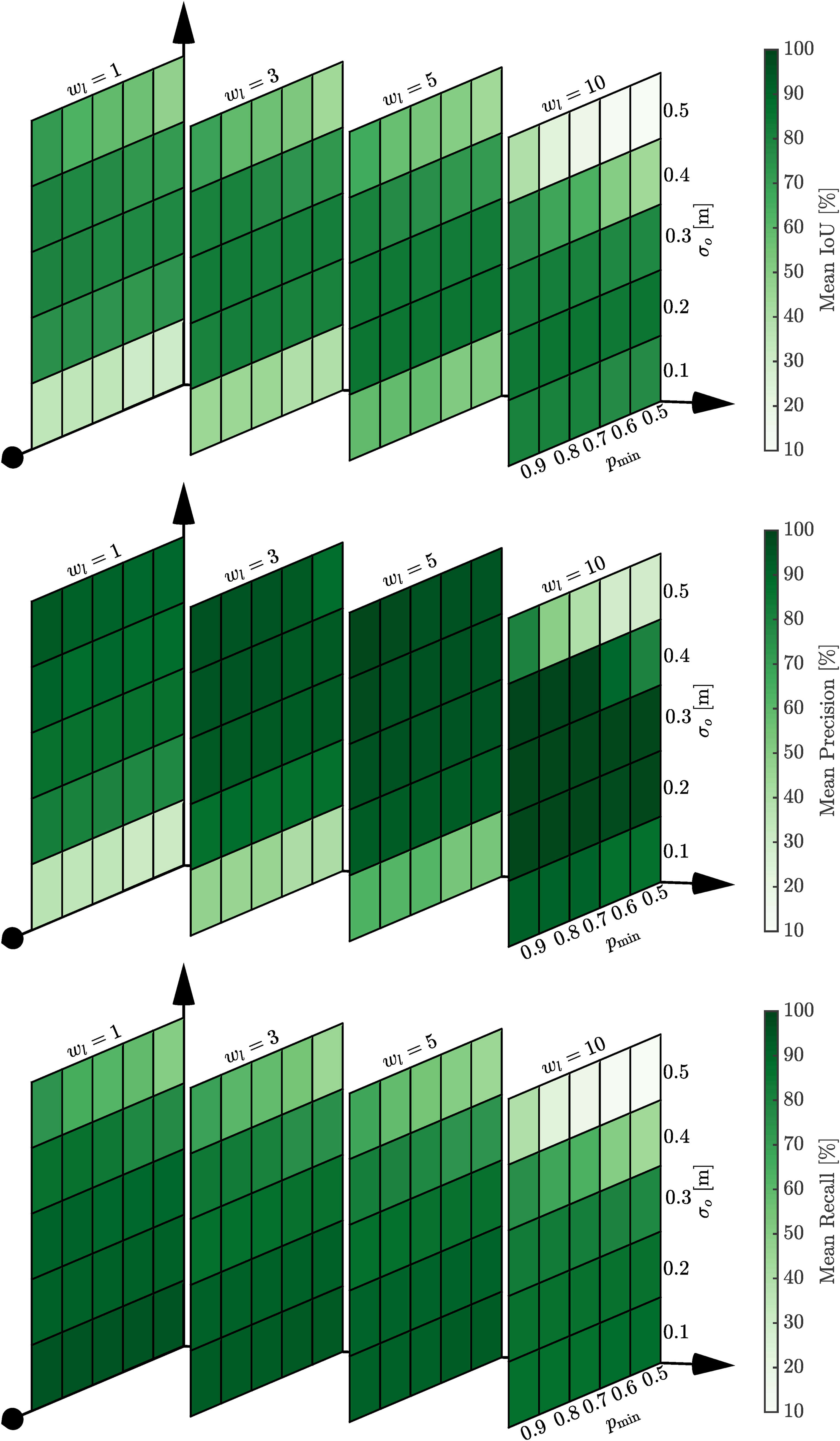

Figure 17 shows the dependency between the size of the convolution kernel, m, the minimum Otsu threshold, γ_min, and the voxel size, Δ. A smaller voxel size allows for finer classification and segmentation of measurements corresponding to dynamic objects. The heatmaps illustrate degraded performance with a large voxel size. Only a single configuration parameter is varied at a time, which contributes to poor performance, as these parameters are interdependent. That is, all three parameters represent physical space. A large voxel size, combined with a large convolution kernel, results in the analysis of a larger area. This explains the poor performance with a voxel size of v = 0.5 and convolution kernel sizes of m = 7 and m = 9. The minimum Otsu threshold filters noisy dynamic detections in static scans. A large value such as γ_min = 4 is shown to reduce performance for a range of voxel sizes. The smallest voxel size continues to perform well, as the dynamic object will occupy more voxels and hence be less affected by the lower threshold.

Figure 17.

The heatmaps show the relationship between the algorithm configuration parameters, m, γ_min, and Δ, on the performance IoU (top), precision (middle), and recall (bottom). A smaller voxel size allows for better performance, but is computationally expensive. All three parameters represent the size of the dynamic detection operation in physical space. A large convolution size, m = 9, results in a high precision, but fails to capture the entire object as reported by the lower recall. The minimum Otsu value is used to filter noisy detections. A large value, γ_min = 4, results in many correct detections being missed. The Shopville (SV) sequence from the DOALS dataset is used for the investigation. The figure is best viewed in colour.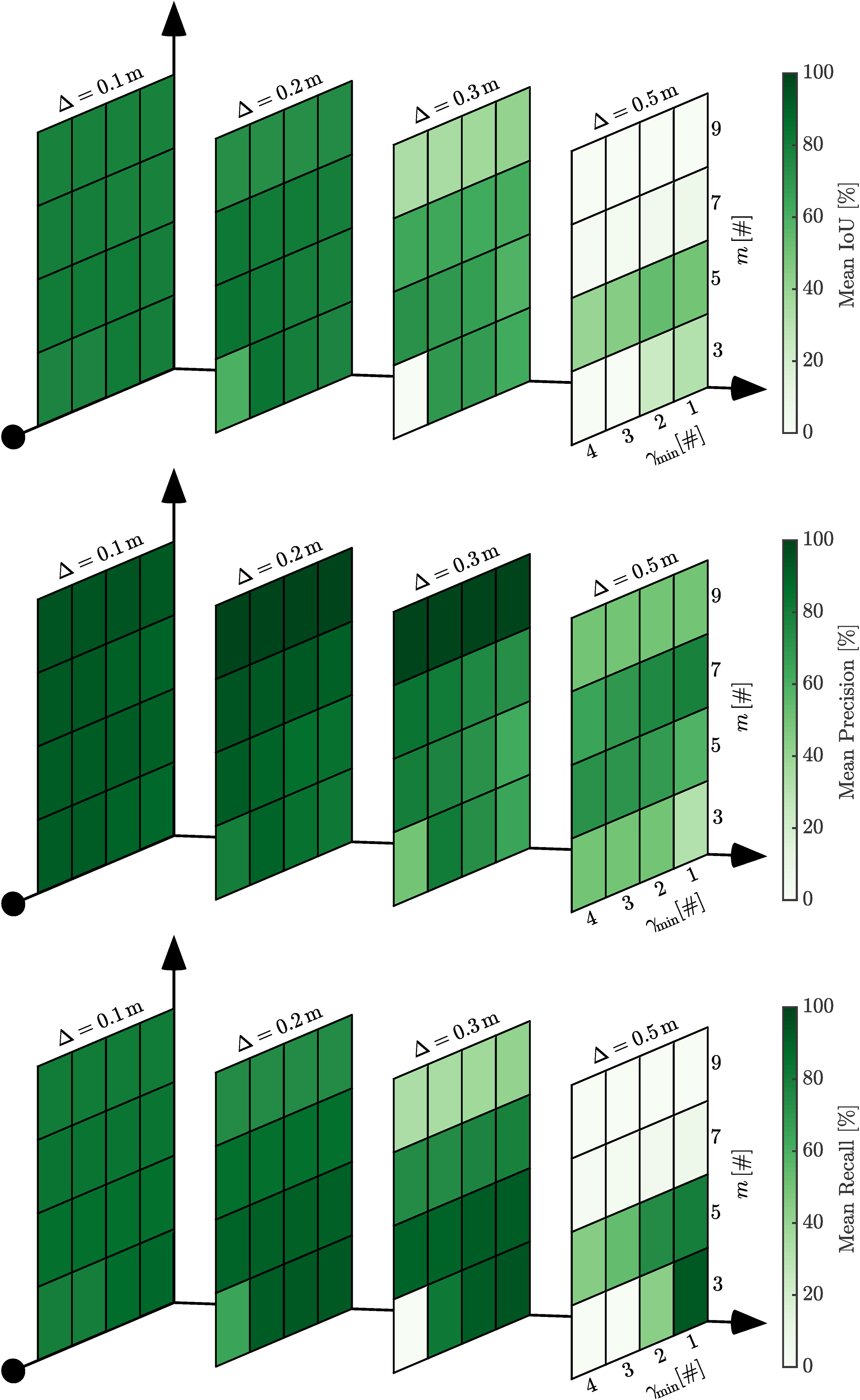

Selecting configuration parameters

The discussion of the proposed MOS pipeline’s stages, visualization of the different algorithm configurations, and analysis of their sensitivity reveal several insights into the effect on the algorithm’s performance. This Section uses these insights to outline an adaptive strategy for selecting the algorithm’s configuration parameters.

Table 1 outlines all algorithm configuration parameters and their purpose. Table 16 provides a guide for their selection, clearly highlighting interdependencies and their recommended values. The default values for the State Update and Local Map are suitable for a range of applications and do not significantly impact MOS performance. The default values provide insight into the relationship between the parameters, with the entries in Table 16 offering a clear guide for their selection. The default parameters provide the desired performance. However, changing the voxel size requires adaptation for all values in the dynamic detection module. Future work involves automatically determining these values online.

Table 16.

A guide for selecting the algorithm’s configuration parameters.

	Parameter	Parameter configuration and selection	Recommendation
State	Transition probability, ϵ	Shown to be insensitive. Both parameters are core to the HMM filter update	It is recommended to use the default parameters
	Transition threshold, pmin
Local Map	Local map radius, rmax	These parameters control the size of the local map used for dynamic detection. The local map radius defines the MOS detection range	It is recommended to use the default global window size, with the map radius configured depending on the desired MOS detection range
	Global window, w g
	Voxel size, Δ	The voxel resolution to discretize space for occupancy representation. A smaller voxel size allows for a detailed representation environment, but at the cost of an increased runtime per frame. The voxel size directly influences the configuration of subsequent dynamic detection parameters	A voxel size of 0.2 m or 0.25 m provide an adequate trade-off between accuracy and speed
Dynamic Detection	Lumped uncertainty, σ o	This value reflects the combined uncertainty in the point cloud measurements and pose estimation accuracy. This value is discretized at the voxel’s resolution	It is recommended to analyze the quality of the sensor’s measurements and the pose estimations to estimate the value of the lumped uncertainty. A dynamic per-scan uncertainty from the sensor’s pose estimate can be used if available
	Convolution kernel size, m	The kernel size used to calculate the convolution score. A small kernel is unable to capture spatial state changes, whereas a very large kernel is unable to capture small detections. The kernel represents a local 3D spatial neighbourhood of voxels over which state changes are accumulated	An intermediate choice of m = 5 is recommended for a voxel size of Δ = 0.2 m (5 × 0.2 = 1 m kernel edge). It is recommended to decrease the kernel size for larger voxel sizes, and vice versa. For example, a voxel size of Δ = 0.1 performs best with m = 7 (7 × 0.1 = 0.7 m kernel edge), whereas a voxel size of Δ = 0.5 m performs best with m = 3 (3 × 0.5 = 1.5 m kernel edge). The kernel size must be an odd integer
	Local window, w l	The convolution kernel is extended over a local window size to compute the 4D convolution. A small window may miss slow or intermittent motion, whereas a large window provides temporal smoothing but may suppress small detections	An intermediate value of three to five scans (0.3–0.5 s at 10 Hz scanning frequency) provides complete detection for most cases. Large windows such as 10 scans, leads to the smoothing of small changes
	Minimum Otsu threshold, γmin	The minimum Otsu threshold is applied to the 4D convolution score: the convolution kernel applied over the local window. This is only introduced for handling noisy detections arising in static scans. The minimum Otsu threshold is physically representing the minimum number of dynamic voxels detected within the kernel across the local window	It is recommended to set the minimum threshold lower than the kernel size to ensure small objects are captured, even if they are only dynamic for portion of the local window

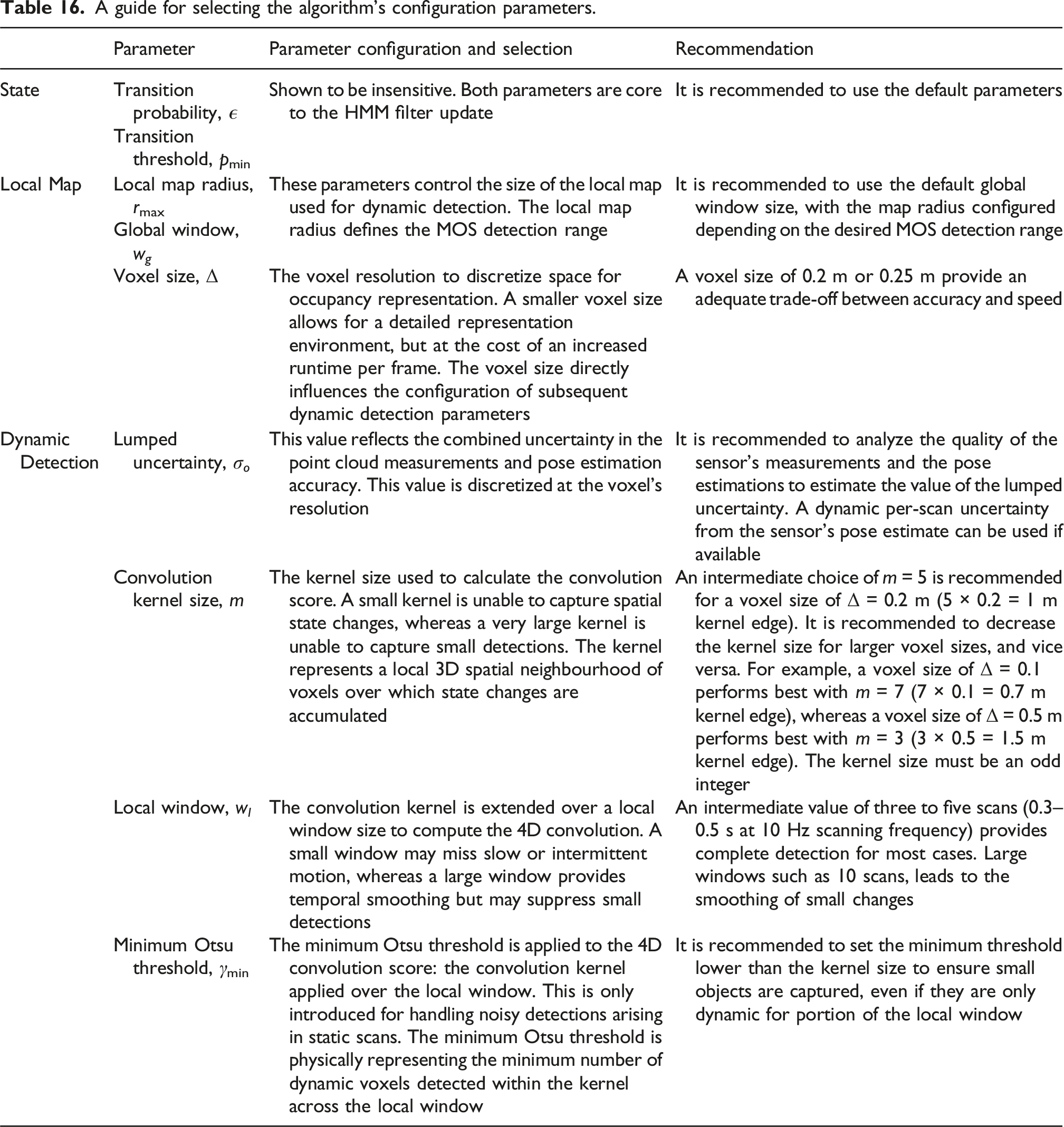
Each of the algorithm’s configuration parameters has a physical meaning. Ill-defined parameters lead to poor performance. The algorithm configuration used for the benchmark tests was tuned using the first Hauptgebaeude sequence from the DOALS dataset during early testing. This allowed the authors to gain an understanding of the parameters and verify beliefs about their dependencies. Upon benchmarking, the configuration was tested with other datasets, resulting in the benchmarked results. We do not see value in optimizing over all nine datasets, as the aim is to design an algorithm that is insensitive to small changes in the configuration and has a meaningful parameter set adaptable for a variety of applications. We invest in describing these relationships to allow for easy and correct adaptation of the algorithm to different applications.

Failure modes

Figure 18 illustrates the failure modes of the proposed approach. Namely, (i) labelling objects moving into unobserved space, (ii) labelling sparse measurements corresponding to dynamic objects, (iii) capturing the complete object, for example, long vehicles such as buses, and (iv) handling large errors in the sensor’s estimated pose.

Figure 18.

The failure modes of the proposed approach include the inability to capture objects moving into unobserved space (top left), differentiating sparse measurements from dynamic objects from noisy detections (top right), capturing the complete dynamic object (bottom left), and handling significant errors, or jumps, in pose (bottom right). The figure is best viewed in colour.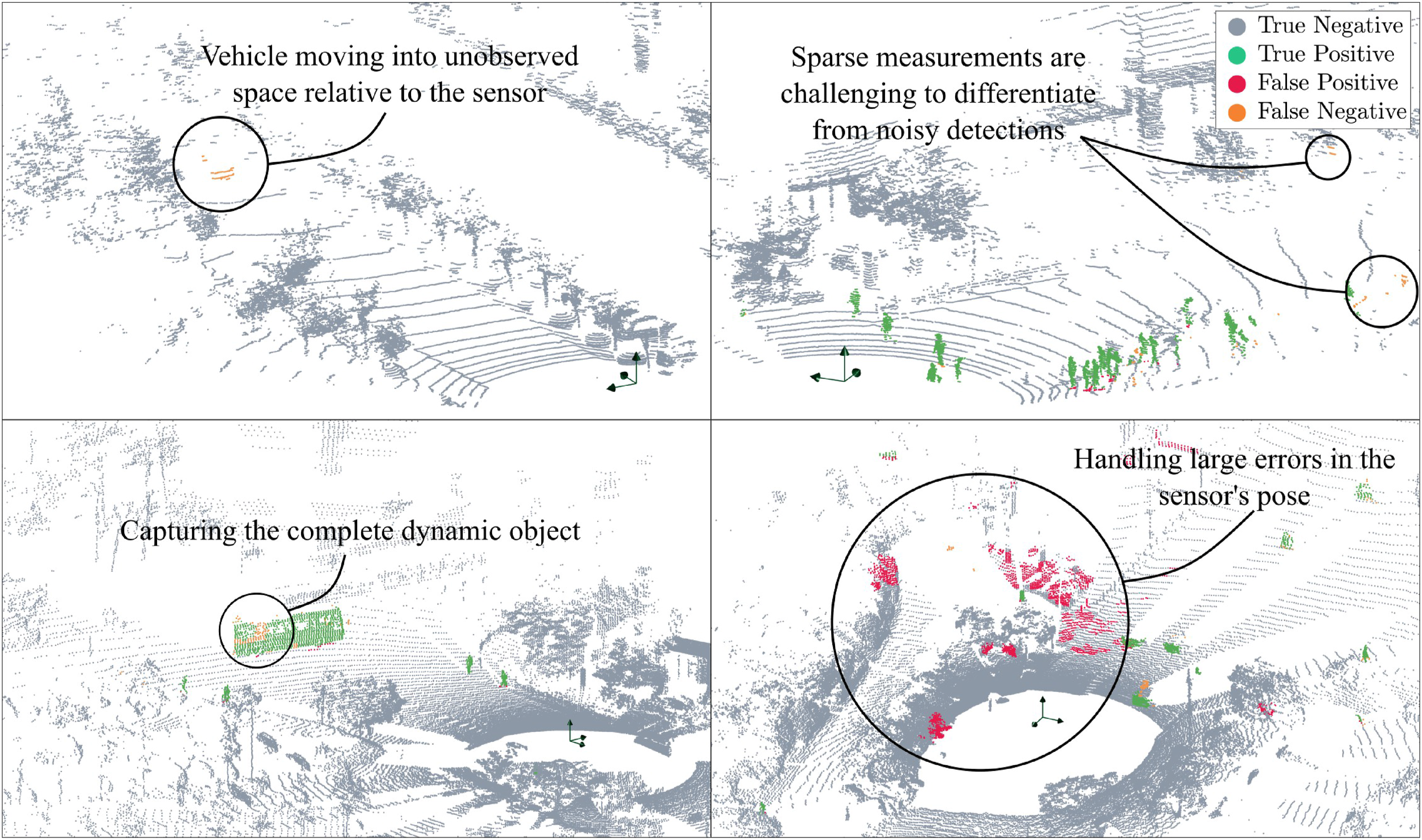

The top left figure shows the failure in identifying dynamic objects moving into unobserved space (see equation (8)). This occurs due to the strict constraints enforced during the 4D convolution, where voxels cannot have unobserved neighbours. The constraint is important as raycasting is known to be inaccurate around the boundary of observed and unobserved space. Other approaches commonly introduce a delay in the detection, for example, 10 scans, to provide better detection around these boundaries.

The top right figure shows a scenario where dynamic labels are missed for sparse measurements. It is challenging to differentiate these measurements from noisy dynamic detections. Consequently, they are rejected in the 4D convolution when using the automatic Otsu thresholding. This failure occurs due to the sensor’s sparse scanning density at longer ranges.

The bottom left corner shows the partial detection of a bus. From a voxel’s perspective, it remains occupied for the entire length of the bus, during which its state does not change. Hence, it identifies the voxel to be static. This failure can be mitigated by introducing the concept of an object rather than examining it at a voxel level only.

The bottom right image shows several false detections occurring due to a significant error in the sensor’s pose. The algorithm depends on an accurate sensor pose locally. That is, large errors or jumps in pose result in incorrect detections, whereas pose drift outside the global window does not impact MOS performance. The probabilistic state update is capable of handling noisy measurements and sensor pose estimates, but large errors cannot be detected in the current implementation.

Future work

The algorithm currently operates at the voxel-level, with the spatiotemporal convolution aiming to capture the complete object. Current approaches use learning-based approaches to identify measurements corresponding to dynamic objects. There is potential to use existing point cloud segmentation methods (Ošep et al., 2024; Xu et al., 2025) in parallel with the proposed approach to allow for complete object detection.

Analysis of the algorithm’s configuration parameters reveals the interdependency between the hyperparameters. A breakdown of the hyperparameters reveals four critical parameters that substantially affect performance: the lumped measurement uncertainty, the convolution kernel size, the local window size, and the minimum Otsu threshold. The other four parameters are either shown to be insensitive (the state transition probability and the state probability threshold) or are for map maintenance only (maximum sensor radius and global window). There is potential to automatically determine the values of the four critical parameters online by analyzing the characteristics of the point cloud data and the operation environment.

The current pipeline uses the lumped uncertainty, σ _o , to capture the uncertainty in the sensor’s pose estimates. Future work involves identifying erroneous pose to avoid false detections. An intermediate module can be introduced to filter poor poses and consequently avoid corrupting the map. Hidden signals, such as significant jumps in the number of estimated dynamic measurements, can be used to identify such instances.

The current algorithm provides accurate MOS detections. However, the MOS range is limited to 25-50 m for real-time results with LiDARs such as the Aeva Aeries II or the Livox Avia. GPU-based solutions can be explored to enable better parallelization of the spatiotemporal convolutions.

Conclusions

Autonomous robots must be capable of detecting dynamic objects. The significant contribution of this work is the provision and demonstration of a solution to the MOS problem that performs as well as, or better than, existing methods, irrespective of the sensor characteristics, platform dynamics, and the robot’s environment. By modelling each voxel as an HMM, the proposed approach allows for confidence-based mapping. The map is queried for changes and facilitates the detection of dynamic measurements. Classic image processing techniques are extended to point cloud data to suppress noisy detections and grow the detection to capture the entire object.

A total of 15 MOS algorithms have been compared across nine datasets, and the proposed algorithm ranks first or second for all datasets. The proposed algorithm ranks first where the ground-truth labels specifically capture movement observed in a scan. Importantly, this is achieved without varying the algorithm’s configuration parameters. A sensitivity study illustrates the motivation for using a probabilistic approach to integrate sensor measurements, and dissecting the pipeline illustrates the benefit provided by each module. The combination of probabilistic modelling using HMMs and 4D convolutions provides a simple approach that works regardless of the inputs and progresses state-of-the-art in labelling moving objects in point cloud data.

The extensive benchmarking conducted in this paper highlights the need for clear and consistent definitions of what constitutes ‘moving’ in a moving object segmentation (MOS) task, along with appropriate benchmarks that enable fair comparison among alternate approaches. We define a moving object strictly as one that is actively in motion during the period of the current scan, not objects that moved previously or might move in the future. While our definition prioritizes instantaneous motion, we acknowledge that this could be extended by definitions that segment objects that have moved in the past or might be expected to move in the future, and these would serve different but equally valid use cases. We propose three classifications of moving objects:

• Objects that are currently moving.

• Objects that have the potential to move.

• Objects that have moved previously and are currently static.

This would allow for consistent performance evaluation. The current confusion of the definition hinders this. We strongly believe this needs to be a consensus decision, not an ex cathedra proclamation.

The establishment of consensus definitions, the creation of consistently labelled datasets, and the development of standardized performance metrics would significantly advance the field. We think this represents an opportunity for collaborative work on datasets labelled by various motion definitions. Inter alia, this would enable meaningful algorithm comparison. The authors welcome approaches from other researchers towards the objective of achieving this.