Active perception network for non-myopic online exploration and visual surface coverage

Abstract

This work addresses the problem of online exploration and visual sensor coverage of unknown environments. We introduce a novel perception roadmap we refer to as the Active Perception Network (APN) that serves as a hierarchical topological graph describing how to traverse and perceive an incrementally built spatial map of the environment. The APN state is incrementally updated to expand a connected configuration space that extends throughout as much of the known space as possible, using efficient difference-awareness techniques that track the discrete changes of the spatial map to inform the updates. A frontier-guided approach is presented for efficient evaluation of information gain and covisible information, which guides view sampling and refinement to ensure maximum coverage of the unmapped space is maintained within the APN. The updated roadmap is hierarchically decomposed into subgraph regions which we use to facilitate a non-myopic global view sequence planner. A comparative analysis to several state-of-the-art approaches was conducted, showing significant performance improvements in terms of total exploration time and surface coverage, and demonstrating high computational efficiency that is scalable to large and complex environments.

1. Introduction

The general problem of online exploration and visual surface coverage of a priori unknown structure or environment can be referred to as online sensor-based coverage planning (OSCP). For this, a robot such as a Micro Aerial Vehicle (MAV) must efficiently discover the spatial and geometric structure of an initially unknown environment using an onboard depth sensor. The robot must traverse the environment to perceive the unknown space from different perspectives, accumulating the acquired sensor knowledge in a spatial map. OSCP is a prerequisite problem for a wide range of applications involving operation in an unknown environment, such as structural modeling and inspection, surveying, search and rescue, and many others (Quattrini Li, 2020).

The global coverage problem of OSCP is to achieve maximum coverage of the target surfaces as efficiently as possible. Naturally, this cannot be solved directly due to the lack of a priori knowledge, and can only be solved online in an incremental fashion. This leads to the incremental exploration problem which represents an iterative action selection problem: given the current incomplete knowledge, determine the optimal action to increase the current knowledge. As each action is executed, the incremental objective is recursively solved using feedback from the added environment knowledge until the global coverage objective has been achieved.

1.1. Related work

The purpose of online exploration and coverage can vary between different applications and tasks. For example, some applications seek knowledge of the traversable space within an unknown environment for subsequent navigation tasks, while others may seek detailed coverage of the surfaces for 3D modeling or inspection purposes. It is important to recognize such differences in the intended application, as this can greatly influence how the problem is approached and how its performance is evaluated.

1.1.1. Frontier-based exploration

Autonomous exploration was pioneered by Yamauchi (1997) by introducing the now well-known concept of spatial frontiers. Frontiers represent boundaries within a partially built map between unknown space the robot seeks to observe, and the free space the robot can use to make the observations. The original frontier exploration algorithm, referred to as classical frontier exploration, was implemented for a mobile ground robot building a 2D occupancy grid map. The algorithm selects the closest frontier as the goal, and navigates toward the goal while using reactive collision-avoidance. Upon arrival, a new sensor scan is acquired of the region and added to the map, repeating the process until no unvisited and reachable frontiers remain.

Many extensions have been proposed to the initial frontier-based approach, including more efficient frontier detection methods (Keidar and Kaminka, 2014; Topiwala et al., 2018) and extensions for 3D maps (Zhu et al., 2015). However, a significant drawback of classical frontier exploration is that frontiers indicate only the existence of adjacent unknown space, but not the quantity or quality. Using a frontier location directly as the navigation goal ignores sensor’s measurement range, thus causing inefficient and wasteful motions. Furthermore, a frontier location near surfaces generally do not represent a feasible goal for a robot due to collision with the surface obstacle, making their direct use in this way ineffective for surface coverage tasks.

1.1.2. Next-best-view (NBV) sampling

Exploration can be effectively modeled as an extension of the Next-Best-View (NBV) problem introduced by Connolly (1985), which can overcome several of the drawbacks associated with classical frontier-based approaches. Here, a view refers to a hypothetical pose of the sensor apparatus used to predict and analyze the spatial information expected to be visible if the real sensor were to be placed at this pose. The expected visible information is then said to be covered by the view.

The classical NBV problem assumed full prior knowledge of the target object is given to facilitate the search and evaluation of NBVs, where the objective was to find a minimum set of views that maximizes coverage of the known surfaces of the object model. This premise can be adapted for online exploration tasks by instead evaluating views according to currently unknown parts of the environment model, rather than the known parts.

Next-best-view (NBV)-based exploration methods typically utilize a generate-and-test paradigm which apply sampling techniques necessary to discretize the continuous configuration space into a finite set of candidate views for analysis (Scott et al., 2003). The quality of a view is evaluated according to some measure of its information gain (IG), which quantifies the new spatial information potentially observable from the view (Heng et al., 2015; Kaufman et al., 2016; Song and Jo, 2018; Stachniss et al., 2005). A cost metric is additionally used to evaluate the expected effort for the robot to visit the view (e.g., time or energy). Most critical differences between existing NBV approaches occur within the sampling strategy for generating view candidates, and the formulation of metrics for analyzing and comparing candidates for goal selection.

Information gain is commonly computed volumetrically by finding the expected amount of unknown space visible from a view (Dang et al., 2019; Kompis et al., 2021; Okada and Miura, 2015). This necessarily involves checking for occlusions within the known space using techniques like raycasting, which incurs high computational complexity that can rapidly increase with various factors like map resolution, sensor field of view, and sensing range. This limits the number of distinct views that can be practically evaluated within a given time period. The high complexity also makes it difficult to analyze overlapping or mutual information between views, such that most approaches treat the gain as an independent value that prevents an understanding of the unique gain contributions of each view within a group.

1.1.3. Tree-based planning

Tree-based methods organize sampled views as vertices in a geometric tree where directed edges between vertices represent feasible paths between views. The RH-NBVP approach of Bircher et al. (2016b, 2018) applies rapidly-exploring random tree (RRT) to grow a tree rooted at the robots current position. Each node in the tree is weighted according to their predicted information gain based on how much unknown space lies within the view. Cost weights are aggregated along each branch, and the leaf node with the highest value is used to identify the best branch to explore, iteratively repeating the process in a receding horizon fashion. This has become a well-known approach and is often used as a baseline for comparative analysis (Cieslewski et al., 2017; Dai et al., 2020; Selin et al., 2019).

A hybrid approach that combines both frontier-based and NBV-based techniques was introduced by Selin et al. (2019), referred to as AEP. It combines the RH-NBVP strategy for local planning, while switching to frontier-based planning for global search when local planning fails to find informative views. FFI (Dai et al., 2020) is also a hybrid approach that uses an efficient frontier clustering strategy to guide view sampling.

A significant drawback of tree-based planning is the difficulty in preserving the previously computed tree structure as the robot navigates to each goal. The RH-NBVP approach builds a new tree each iteration, discarding the previously built structure that may still contain useful knowledge. Other approaches attempt to transfer as much of the previous tree structure as possible by rewiring its edges to initialize the construction of a new tree. Since tree-based methods are rooted at the robots position, they tend to become increasingly inefficient over larger distances, making it difficult to handle dead-end or backtracking cases.

1.1.4. Graph-based planning

Various approaches have utilized graph structures that can overcome some of the limitations and drawbacks of trees. The approach of Witting et al. (2018) builds a history graph that stores previously visited positions and their edge connections. These are used as potential seed points for RRT, which allows a tree to be grown from different positions across the map, rather than just from the robot position. An approach using Rapidly-Exploring Random Graphs (RRG) was presented in Dang et al. (2019) for exploration of subterranean environments. A Probabilistic Roadmap (PRM) strategy was used by Xu et al. (2021) to build a graph of feasible configurations and paths over the map as it is explored.

1.1.5. Topological maps

Topological maps have been applied by recent works which aim to reduce the planning complexity through the compact representation provided by a topological map. Topological maps can be considered as an extension to graph-based methods, where vertices represent some volumetric sub-map, or place, and edges represent the adjacency or reachability between places. This coarse and abstracted representation is more efficient for handling large-scale environments, which can become intractable to explore online using alternative approaches. However, they usually lack sufficient metric knowledge for direct use in navigation.

A topological map was used by Silver et al. (2006) for exploration of underground mines by a ground robot. The regions of intersection between passageways were represented as nodes, and exploration was planned along the edges between nodes.

Other approaches have applied spatial partitioning of the known free space to identify a topological map structure. A contour-based segmentation approach was presented by Fermin-Leon et al. (2017) to decompose a 2D occupancy grid into polygonal regions corresponding to meaningful regions like corridors or rooms of a building. Yang et al. (2021) used convex polyhedra to decompose a 3D map into distinctive exploration regions for subterranean exploration. A uniform decomposition method was proposed by Cao et al. (2021) which partitions space into even cuboid subspaces.

1.1.6. Myopic greedy planning

The majority of existing methods compute navigation goals using myopic planning strategies that greedily optimize the cost of the next single planning decision (Dai et al., 2020; Palazzolo and Stachniss, 2018), or within a limited planning horizon (Bircher et al., 2016b; Selin et al., 2019). Some works allow planning to search for goals using the full map, but still consider only the local costs and independent rewards of each goal and apply greedy search strategies. These are sometimes referred to as global planning methods, but we clarify they are still considered myopic.

Myopic strategies bias exploration toward regions with high information gain, while ignoring small gains even if they are closer. This bias can frequently create regions of incomplete coverage when a high-gain goal leads the exploration away from the current region before it is fully mapped. This can also result in frequent back-and-forth oscillation between goals, or require re-visitation of these regions after the robot has traveled a significant distance, backtracking over potentially large distances. This greatly reduces efficiency, and can result in sparse coverage gaps or failure to fully explore an environment within an allowed time limit, especially over large-scales.

1.1.7. Non-myopic planning

Non-myopic planning has been referred to using several names, such as view path planning or informative path planning (IPP). It can be effectively formulated using variations of the Traveling Salesman Problem (TSP) or shortest Hamiltonian path problem which seek an ordered exploration path that optimally explores the remaining unknown parts of the map. In this way, planning can account for the conditional information gain of each path point, dependent on the information and costs along the previous parts of the path. Offline approaches using such formulations have been developed (Bircher et al., 2016a; Shang et al., 2020) when a prior map is available, but are infeasible for online applications which require iterative replanning as the map evolves.

Online global and non-myopic planning has only been considered by a relatively small number of recent papers.

A sector decomposition approach was presented by Song et al. (2020), which partitions the map into a set of convex sectors used to compute a TSP sequence. However, the sector decomposition method is computationally expensive, especially for finer map resolutions, which can greatly decrease the update rate of the map and planning. Additionally, sectors form an exact partitioning of the space, which can make the geometric properties of the resulting sectors difficult to control, and can result in a large number of sectors that cannot be handled over large-scale and complex environments.

Zhou et al. (2021) developed a hierarchical planning approach based on a novel frontier information structure. Frontiers are globally clustered and used to estimate a global exploration route, planning a more detailed view sequence within a local horizon.

A hierarchical planning approach presented by Cao et al. (2021) partitions the map into even cuboid subspaces to build a topological map. Global planning operates by finding the sequence to visit each subspace, using A* to search for minimum-cost paths connecting subspaces. Local planning then operates at higher resolution within the current subspace about the robot to find an ordered sequence of views to maximize coverage of the local subspace.

However, a drawback of these forms of top–down decomposition is that they can arbitrarily divide regions of the map without considering the underlying reachability within the environment; the information content of each subspace and its candidate views are secondarily evaluated. When a global plan is computed, the executed traversal cost may differ greatly from the estimated cost between the regions. For example, a region A may contain information only visible from a view in an adjacent region B. This will only be discovered once region A is visited, and thus it fails to accurately anticipate the future action costs. Also under some conditions, such as highly complex geometries of the environment, certain subspaces can be way more complex than some other subspaces, which can lead to inefficient coverage paths. For several of the cited works, the underlying metric space may not be explicitly represented (e.g., using a graph or roadmap). Path searches thus operate directly on the map, and may need to be recomputed from scratch in each update. This can become too expensive at large scales or fine resolutions, potentially restricting their applicability.

1.1.8. Environment and task-specific constraints

Simplifying or restrictive assumptions are sometimes made on the operational environment. This can include indoor operation, or reliance on certain regular geometric features, for example, room structures used for segmentation. Some applications are intended to operate in relatively obstacle-free environments, such as outdoors or underwater (Ellefsen et al., 2017), which contain an abundance of free-space that greatly simplifies collision checking and other sub-tasks. Others assume the environment can be explored along a relatively planar path, which helps reduce the dimensionality, but may become infeasible for applications that extend throughout all spatial dimensions. Assumptions can significantly restrict the practicality of many approaches for general use, or require fine tuning of parameters between different environments to achieve their rated performance.

1.1.9. Limitations of existing approaches

Limitations of existing approaches are summarized as follows:

• Greedy and myopic planning strategies that focus on the incremental exploration objective, but fail to consider the global one,

• Non-generalized approaches that are limited to small-scale environments, or specialized for specific environments or conditions (e.g., subterranean or building-like structures),

• Most approaches succumb to high computational costs:

– They do not scale well with respect to environment size or map resolution,

– The ability to quickly replan on added knowledge diminishes, where a suboptimal plan is fully executed before replanning,

– Reduced velocities are often required to compensate for low planning rates,

– Frequent stop-and-go motions can occur.

There is currently a lack of modular and generalizable software to sufficiently overcome the aforementioned limitations. Online exploration involves many interacting subsystems and maintenance of large amounts of dynamically changing data structures, often with dependencies between different forms of dynamic data. Fully designing such a system is a large-scale and time-consuming development task, often requiring high levels of programming expertise that not all researchers may possess. To compensate, most researchers tend to reduce the development burden by ignoring software aspects like reusability, maintainability, and extensibility, where the resulting software becomes highly coupled to the formulations and specifications of their specific approach (Kortenkamp et al., 2016). This is known as technical debt (Suryanarayana et al., 2014). In consequence, the software has low reusability to other researchers with different specifications, and thus they can use the same development approach that repeats this cycle. In practice, software challenges can create an entry barrier leading to a bottleneck to the rate of research progress for online exploration and similar problems, and they also make benchmark analysis very difficult.

1.2. Contributions

This work is motivated to alleviate some of the limitations of the existing approaches in handling the OSCP problem. We focus first on how to dynamically compute and maintain the accurate global knowledge necessary to a non-myopic planning algorithm, since this represents a significant bottleneck in terms of computational complexity and exploration quality in the existing work. Our key contributions are as follows:

• A novel dynamic multi-layer topological graph designated as the Active Perception Network (APN). The APN serves as a global hierarchical roadmap over the spatial map that accumulates the incrementally computed knowledge of the exploration space. It is defined and organized around adaptive nodes to best represent the perceptual and actionable environment knowledge discovered to minimize the complexity, which allows it to be efficiently accessed and searched for planning purposes.

• A dynamic update procedure referred to as Differential Regulation (DFR) to incrementally build and refine the APN as environment knowledge is increased. This procedure addresses the complexity of updating the APN as its size and the map scale increase, while ensuring sufficient global knowledge is maintained for effective planning.

• A non-myopic planning approach denoted as APN-Planner (APN-P) that demonstrates how the APN can be leveraged to compute and adaptively refine a globally informed exploration sequence.

• A detailed performance analysis and comparison to existing approaches among the state-of-the-art.

• An open-source release of our Active Perception for Exploration and Mapping (APEXMAP) software framework, which was used to implement the APN, DFR, and APN-P. This framework is designed to address exploration and active perception in a generalized and reusable fashion. It factorizes the general aspects of the problem domain into modular components that enable rapid development of a wide range of approaches. This contribution is intended to reduce the existing entry-barriers for online exploration and active perception research.

2. Problem formulation

We assume exploration is performed using an MAV equipped with an onboard depth sensor (e.g., stereo-visual, RGB-D, or LiDAR) to perceive 3D space, noting that other systems such as mobile ground robots could also be utilized without loss of generality. We define the following terms and symbols to facilitate the description of our approach.

2.1. Environment and map model

Let $\mathcal{W}\subset {\mathbb{R}}^3$ represent the bounded 3D space of the operational environment, referred to as the world. The solid structures and objects of the world represent occupied space ${\mathcal{W}}^{occ}\subset \mathcal{W}$ , while the remaining volume is defined as free-space ${\mathcal{W}}^{free}\subset \mathcal{W}$ , such that $\mathcal{W}\equiv {\mathcal{W}}^{free}\cup {\mathcal{W}}^{occ}$ .

The intersection boundaries between occupied and free-space define the surface manifolds, $\mathcal{S}\subset {\mathbb{R}}^2$ . Surface manifolds are assumed to be visually opaque, and a surface point is considered optically visible from a point $\mathit{x}\in {\mathcal{W}}^{free}$ only if no occupied space lies between the surface and x . Otherwise, the surface is considered to be occluded from x .

A spatial map $\mathcal{M}$ is used to store the environment state knowledge as it is discovered from sensing. We assume the use of a 3D grid-based occupancy map $\mathcal{M}=\left\{{\mathit{m}}_0,\dots ,{\mathit{m}}_m\right\}$ , though other map models could also be used without loss of generality (e.g., Signed Distance Field (SDF) (Oleynikova et al., 2017)). $\mathcal{M}$ partitions $\mathcal{W}$ by a set of non-overlapping cubic volumes $\mathit{m}\in {\mathbb{R}}^3$ , known as voxels. The minimum edge length of a voxel dictates the map resolution, $r_{\mathcal{M}}$ .

Each voxel stores the occupancy probability of its volume, which is updated from sensor measurements depending on whether occupied or free-space was observed. The probability value is discretized by an occupancy state $\mathcal{O}\in \left\{{\mathcal{O}}^{unk},{\mathcal{O}}^{occ},{\mathcal{O}}^{free}\right\}$ , where ${\mathcal{O}}^{unk}$ indicates the state is unknown. As sensor measurements are integrated, the state is classified as either ${\mathcal{O}}^{occ}$ or ${\mathcal{O}}^{free}$ to indicate, respectively, whether the voxel belongs to the set of occupied voxels ${\mathcal{M}}^{occ}\subseteq \mathcal{M}$ or free-space voxels ${\mathcal{M}}^{free}\subseteq \mathcal{M}$ . The set of occupied voxels are given as ${\mathcal{M}}^{occ}\subseteq \mathcal{M}$ , the set of free voxels is given by ${\mathcal{M}}^{free}\subseteq \mathcal{M}$ , and the set of unknown voxels is given by ${\mathcal{M}}^{unk}\subseteq \mathcal{M}$ , with the initial map state given as $\mathcal{M}\stackrel{\text{init}}{=}{\mathcal{M}}^{unk}$ .

Spatial frontiers, $\mathcal{F}$ , are detected from $\mathcal{M}$ by identifying unknown voxels with an adjacent free voxel. Frontiers that are also adjacent to an occupied surface voxel are further classified as surface frontiers, ${\mathcal{F}}^{\mathcal{S}}$ . Those that are adjacent only to free space are classified as void frontiers, ${\mathcal{F}}^{\mathcal{X}}$ , such that $\mathcal{F}\equiv {\mathcal{F}}^{\mathcal{S}}\cup {\mathcal{F}}^{\mathcal{X}}$ . These distinctions are made according to the goal of achieving complete surface coverage, where surface frontiers help to identify where surface coverage is incomplete.

2.2. Robot model

The robot agent is modeled by a rigid body with pose configuration q ^agent (t) = ( x , a ), q ∈ SE(3) at time t, where $\mathit{x}\in {\mathbb{R}}^3$ is the position vector and a = {φ, ϑ, ψ} is the orientation vector represented by roll, pitch, and yaw Euler angles, respectively. Additional parameters v _max and ${\stackrel{.}{\psi }}_{\mathit{max}}$ are used to specify the maximum allowable velocity and yaw rate, respectively. A spherical volume B ^safe centered at x with radius d _safe is defined, where d _safe specifies the minimum obstacle separation distance for safe operation.

2.3. Sensor model

The robot’s depth sensor is modeled by the parameter vector $\left[R_s,{\alpha }_s,d_{\mathit{max}}^{sense}\right]$ . α _s = [α _h , α _v ] ∈ (0, 2π] is the maximum angular field of view (FoV) on the horizontal and vertical dimensions of the sensor, and R _s = [R _sx , R _sy ] is the maximum spatial resolution. $d_{\mathit{max}}^{sense}\mathbb{\in }\mathbb{R}$ is the maximum effective sensing range that surface points can be accurately detected by the sensor. This value corresponds to the physical limitations of the sensor, where distances greater than $d_{\mathit{max}}^{sense}$ either cannot be measured, or are rejected due to loss of accuracy.

The sensor parameters can be combined with a pose q to form a projection model λ ∈ Λ, referred to as a viewpose. The projected space from λ is described by the subset of rays that pass through the view’s origin x , constrained by the intervals [ϑ ± α _v /2] and [ψ ± α _h /2] of the unit-sphere. The length of each ray is constrained by $d_{\mathit{max}}^{sense}$ . The projected space defines the view volume of a viewpose, and a location within the view volume is considered visible if there are no occlusions between it and the origin. This provides the basis for making visibility queries and predictions on the expected information gain.

2.4. Reachable configuration space

Given the robot’s initial position ${\mathit{x}}_0^{agent}$ , the reachable configuration space $\mathcal{X}\subset {\mathbb{R}}^3$ is a metric space defined by all admissible configurations path-connected to ${\mathit{x}}_0^{agent}$ . As a precondition, a configuration is considered admissible if it does not intersect any occupied space within distance d _safe . It is then considered reachable if there exists a simply-connected path of admissible configurations from ${\mathit{x}}_0^{agent}$ . The distance between two reachable points is quantified by a metric value $L\mathbb{\in }\mathbb{R}$ .

2.5. Goal space

The surfaces that can possibly be covered at any point during exploration are inherently restricted to a subset ${\mathcal{S}}_{\mathcal{X}}\subseteq \mathcal{S}$ which are visible from some viewpose λ constrained by $\mathcal{X}$ . The goal space Λ ^G ⊂ Λ is then defined as the set of feasible configurations that contribute some amount of coverage of ${\mathcal{S}}_{\mathcal{X}}$ , quantified by a gain metric, $\gamma \mathbb{\in }\mathbb{R}$ .

2.6. Exploration state space

The exploration state space, Ω, refers to the collectively available knowledge necessary to solve the incremental exploration problem. This mainly consists of the robot pose q ^agent , spatial map $\mathcal{M}$ , and frontiers $\mathcal{F}$ , which are considered as independent time-varying input variables. It additionally includes the reachable C-Space, $\mathcal{X}$ , and goal space, Λ ^G , which are dependent variables computed from the input data.

2.7. Myopicity

A planning strategy operates on the exploration state space to search for the optimal goal q ^g ∈ Λ ^G for navigation, where the myopicity corresponds to the length of its planning horizon. A myopic strategy typically uses greedy search techniques which treats each goal or action as independent of the others, greedily selecting the best one. They may also constrain the search to only some local sub-region of the map, rather than considering its full extent. Myopic strategies focus on the optimization related to the incremental exploration problem, which are not necessarily optimal with respect to the global coverage objective.

In contrast, a non-myopic strategy searches over a long horizon that spans most or all of the available map. It additionally considers how the particular selection of a goal and its associated action may alter the future exploration state space. This involves search and evaluation over ordered sequences of actions, rather than each action individually. This results in solutions that are more optimal with respect to the long-term global coverage objective.

3. Methodology

We will start with an overview of our approach and then describe each important component of the approach in turn.

3.1. Approach overview

In this work, we address how to build a reusable exploration state space Ω that is adaptively maintained over the full spatial map as it is built concurrently. The iteratively built exploration space is then used to facilitate efficient non-myopic planning. We seek an approach that generalizes well to different environments with varying complexities and geometric characteristics, and efficiently scales to large-sized environments that cannot be effectively solved by myopic approaches.

To achieve this goal, we introduce a novel graph-theoretic information structure named the Active Perception Network (APN) to model the exploration state space data, detailed in Section 3.2. A key feature of the APN is a hierarchical decomposition that allows the underlying graph structure to be simultaneously represented by a reduced-size topological map.

In contrast to the top–down decomposition methods used in other works, the APN uses a bottom–up approach where the high resolution reachability, visibility, and other information is built and maintained globally, and the high-level topological subspaces are then computed from the low-level structure. This allows the formation of topological regions to be guided by the actual traversability and costs of the underlying space. Thus, the visible information of each subspace is implicitly captured in terms of the actual configurations and the associated traversal costs to observe it. Furthermore, subspaces do not form a dense space partition, instead they can be focused around only the data of interest, reusing the underlying edge structures to perform traversal between subspaces.

Another focus of the APN is the storage, organization, and analysis of the contained data, such that dynamic changes can be efficiently made to any of its contents as its size increases, while also maximizing the low-level efficiency for search and query operations. These aspects relate to optimization of the running time computation efficiency, which is related to software, data structures, and other implementation aspects. However, these technical implementation details are largely beyond the scope of this work; instead, the APN will primarily be described from a modeling perspective, with some additional implementation details provided in the Appendix.

We additionally introduce the process of Differential Regulation (DFR) in Section 3.3, which operates on the APN to modulate its state with respect to the increasing map knowledge. DFR consists of sampling-based methods for increasing knowledge of the goal space and reachable space. A novel approach for information gain analysis is utilized that enables the individual and mutual information gain of the APN to be efficiently computed, which is leveraged to accelerate informative view sampling, pruning, and refinement.

Differential Regulation (DFR) exploits the incremental nature of map building where each sequential map update induces changes that occur only within a relatively small local region of bounded volume, independent of the total map size. With this insight, these incremental changes are tracked and cached using difference-awareness and memorization strategies to greatly reduce the computational overhead necessary to update the APN. This allows more discrete updates to be performed in a given time period, increasing the completeness and accuracy of each update. The ability to quickly perform each update is also critical to ensure the size of the map changes remain small, since the complexity of each update scales with the size of the changes.

An anytime exploration planner is presented in Section 3.4, which demonstrates the use of the APN to efficiently compute non-myopic global exploration sequences. The hierarchical representation of the APN is leveraged to first compute a global topological exploration plan over the full map. The beginning of the global plan is then locally optimized at a higher-resolution. Similar to the difference-aware approach used by DFR, sequential changes to the APN typically occur within locally bounded regions which are leveraged to initialize new planning instances from previous results. This allows optimizations to achieve faster convergence despite the increasing size of the map and APN.

The iterative exploration pipeline is illustrated in Figure 1, which consists primarily of two asynchronous processing loops. The first loop is dedicated for spatial mapping to allow continuous integration of the sensor measurement data, Z _t , at high frequency. Frontier detection is performed after each map update, which operates only on the state-changed voxels that resulted from the update. This minimizes the complexity required to maintain the global frontier set, and provides a constant upper complexity bound that remains independent of the total map size. The second loop concurrently performs DFR to update the APN, which then serves as the input for replanning the current exploration solution. Further details of each DFR subroutine will be provided in Section 3.3.

Figure 1.

Mapping, frontier detection, and Differential Regulation process pipelines used to update the APN.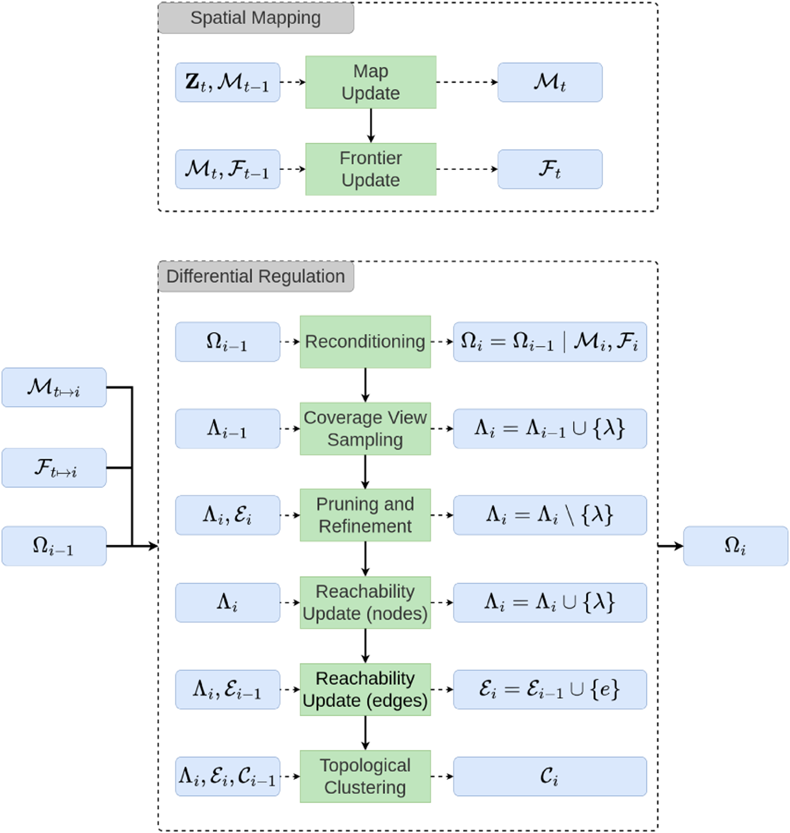

3.2. Active perception network (APN)

The Active Perception Network (APN) serves as a topological roadmap that stores the unified knowledge of the dynamically exploration state space. Its fundamental structure is represented by a hypergraph

$\mathcal{G}=\left(\mathcal{V},\mathcal{E},\mathcal{C}\right),$

(1)

where $\mathcal{V}={\left\{v_i\right\}}_{i=1,\dots ,n}$ is the set of graph nodes and $\mathcal{E}={\left\{e_{u,v}\right\}}_{u,v\in \left[1,n\right]}$ is the set of traversal edges between nodes. The nodes have a bijective mapping to a codomain of viewposes, $\mathcal{V}\hookrightarrow \mathrm{\Lambda }$ , where the terms node and viewpose may also be referred to interchangeably. $\mathcal{V}$ is decomposed by a set of hyperedges $\mathcal{C}=\left\{\mathcal{H}\right\}\in \mathcal{P}\left(\mathcal{V}\right)$ , where $\mathcal{P}$ is the power set. Each hyperedge $\mathcal{H}\subseteq \mathcal{V}$ contains a disjoint subset of $\mathcal{V}$ as a multi-level hierarchy.

Graph nodes, $\mathcal{V}$ : Each node $v_i\in \mathcal{V}$ represents a viewpose information structure that consists of the tuple

$v_i=\left\{{\mathit{q}}_i,{\gamma }_i,{\mathbb{1}}_i^{open}\right\},$

(2)

where q _i is its pose which has an associated viewpose q _i ↦λ _i , and ${\gamma }_i\mathbb{\in }\mathbb{R}$ is a reward metric that quantifies the expected information gain available from λ _i . The node’s visitation state is stored by a Boolean indicator ${\mathbb{1}}_i^{open}:v_i\mapsto \mathbb{B}$ , corresponding to whether the robot has visited the pose of v _i . A true value indicates the node is unvisited, also referred to as open, and is otherwise referred to as closed if it has already been visited. This is used to discriminate between the open set of nodes ${\mathcal{V}}^{open}$ which can represent goal candidates, and the closed set ${\mathcal{V}}^{closed}$ of nodes which have already been visited.

Several important classifications are defined over $\mathcal{V}$ based on their properties. These provide an increased understanding of how the network can serve different tasks. These are summarized as follows:

• A unique node $v^{agent}\in \mathcal{V}$ , referred to as the agent node, is used to represent the robot and is dynamically updated with the robot pose as it changes over time. The robot’s initial pose ${\mathit{q}}_0^{agent}$ is used to define the home state, represented by a unique node v ^home that remains fixed over the lifetime of the APN.

• The previously traversed path of the robot is represented by a path-connected set of keyframe nodes, ${\mathit{q}}_{0:t}^{agent}\mapsto \left\{v_{0:k}^{kf}\right\}\in {\mathcal{V}}^{kf}$ , rooted at the home state, $v_0^{kf}=v^{home}$ . Keyframe nodes are added in intermediate intervals once the robot has traveled a minimum distance from the last keyframe.

• Unvisited nodes with positive information gain are classified as NBV candidate nodes, represented by the set ${\mathcal{V}}^{nbv}=\left\{v\in {\mathcal{V}}^{open}:\gamma \left(v\right)>0\right\}$ . A Next Best View (NBV) node represents a subgoal candidate for for navigation and planning that is expected to increase map knowledge.

• The remaining traversal nodes, ${\mathcal{V}}^{\mathcal{X}}=\mathcal{V}\setminus {\mathcal{V}}^{nbv}$ , mainly serve to preserve the accumulated knowledge of the reachability space and its connectivity, but not expected to increase map knowledge.

Graph edges, $\mathcal{E}$ : Each edge $e_{u,w}\in \mathcal{E}$ corresponds to the pair of nodes ⟨v _u , v _w ⟩, and stores various analytical information of the traversal space between the pair as follows:

$e_{u,w}=\left\{d^{\mathit{x}},d^{\psi },\mathcal{D},OBB,l^{\mathcal{O}},{\mathit{p}}^{obs}\right\},$

(3)

where d ^x and d ^ψ are the Euclidean distance and the orientation angle distance, respectively, between (v _u , v _w ). $\mathcal{D}$ is the evaluated cost metric value to traverse the edge given the maximum velocity v _max and yaw rate ${\stackrel{.}{\psi }}_{\mathit{max}}$ , defined by:

$\mathcal{D}\left(e_{u,w}\right)=\mathit{max}\left(\frac{d^{\mathit{x}}\left(e_{u,v}\right)}{{\mathit{v}}_{\mathit{max}}},\frac{d^{\psi }\left(e_{u,v}\right)}{{\dot{\psi }}_{\mathit{max}}}\right).$

(4)

Each edge also stores the Oriented Bounding Box (OBB) enclosing the endpoints, and the collision state of the space contained in the OBB is stored by $l^{\mathcal{O}}:OBB\to \left\{free,unk,obs\right\}$ . p ^obs is used as a memory cache that stores any uncertain voxels found from previous collision checks. This allows for lazy evaluation during future checks by first checking if these discrete voxels have changed, rather than the full OBB volume, to greatly reduce computations. We note that, in this implementation, rewards are not explicitly computed for edges for efficiency purposes.

3.2.1. Hyperedge clusters

A set of hyperedges $\mathcal{C}\subset \mathcal{P}\left(\mathcal{V}\right)$ forms a topological decomposition of $\mathcal{G}$ , providing a more compact representation of the underlying space that is more efficient for high level operations where high level-of-detail is not essential. A hyperedge $\mathcal{H}\in \mathcal{C}$ represents a cluster of nodes $\left\{v\right\}\subseteq \mathcal{V}$ grouped according a similarity measure between the nodes, such that $\mathcal{C}$ is a partitioning of $\mathcal{V}$ into disjoint subsets $\left\{\mathcal{H}\right\}$ . Each hyperedge is modeled by the following:

${\mathcal{H}}_i=\left\{{\mathcal{V}}_i^{\mathcal{C}},{\mathcal{A}}_i,B_i,{\mathit{x}}_i\right\},$

(5)

where ${\mathcal{V}}_i^{\mathcal{C}}$ is the set of nodes belonging to ${\mathcal{H}}_i$ , with the centroid of the contained nodes given by x _i and its bounding volume given as B _i . ${\mathcal{A}}_i=G\left[{\mathcal{H}}_i\right]$ is the vertex-induced subgraph formed by each cluster containing the clustered nodes $v\in \mathcal{H}$ and the induced edges $\left(e_{u,w}\in \mathcal{E}:v_u,v_w\in {\mathcal{V}}_i^{\mathcal{C}}\right)$ with both endpoints belonging to A _i .

Induced edges of a cluster $\mathcal{E}\left[{\mathcal{H}}_i\right]$ are referred to as its interior edges, while the remaining edges $\mathcal{E}\setminus \mathcal{E}\left[{\mathcal{H}}_i\right]$ that connect different cluster groups are referred to as exterior edges. The efficiency of global search queries and traversal through $\mathcal{G}$ can greatly increased by traversing between subraphs using their exterior edges, using the interior edges of the subgraphs to perform local operations as needed.

3.3. Differential regulation

The APN is incrementally built by the process of Differential Regulation (DFR), which manages how information is added, removed, or modified in the APN with respect to the concurrently built spatial map. DFR evaluates the APN according to a set of objectives and constraints conditioned on the current map and executes a set of modifying procedures on the APN as needed to ensure they remain satisfied as the map evolves.

The broad purpose of the DFR procedures is to (a) re-evaluate map-dependent analytical measures to ensure their accuracy (e.g., information gain of existing nodes), (b) add node and edge elements to increase the completeness of the network while pruning redundant or overcomplete elements, and (c) recompute the topological clustering of the updated graph state. A diagram of these procedures is shown in Figure 1, and detailed in the following subsections.

3.3.1. Reconditioning

Each DFR cycle i begins at a time t with the latest spatial map ${\mathcal{M}}_{t\left(i\right)}$ , frontiers ${\mathcal{F}}_{t\left(i\right)}$ , and robot pose ${\mathit{q}}_{t\left(i\right)}^{agent}$ . The first task is to determine the local differences of these variables to their states from the previous cycle t(i − 1). Each incremental map update reports the set of state-changed voxels, which are accumulated in a local cache $\mathrm{\Delta }\mathcal{M}$ with its bounding volume ΔB. This is defined as the local difference neighborhood and is used to inform various APN update procedures about where state-changes have occurred, described further in the next subsections.

Each regulation cycle then begins by updating the pose of the agent node v ^agent and its local edges. The length of the local path is then checked and compared against a keyframe threshold distance. If the threshold is exceeded, a new keyframe view v ^kf is created from v ^agent and added to the keyframe set ${\mathcal{V}}^{kf}$ , with an edge connection to the previous keyframe to ensure a connected path to the home location is always maintained.

3.3.2. View analysis and coverage sampling

View analysis and coverage sampling ${\mathcal{V}}^{nbv}$ represents the set of NBV subgoal candidates expected to observe currently unknown voxels, such that map coverage will be increased if a subgoal is visited by the robot. To support the purposes of non-myopic planning, ${\mathcal{V}}^{nbv}$ should be sufficiently distributed to provide maximum coverage of the unknown map space. Additionally, maximum coverage should be achieved using a minimal size of ${\mathcal{V}}^{nbv}$ to reduce the eventual planning complexity that can increase rapidly with the number of views considered.

A sampling-based approach is used to incrementally build ${\mathcal{V}}^{nbv}$ to maintain maximum coverage as the map evolves. To efficiently and scalably achieve the aforementioned characteristics desired of ${\mathcal{V}}^{nbv}$ , we introduce an approach using a frontier-based heuristic to evaluate information gain and also guide the sampling of additional views.

3.3.2.1. Information gain analysis

A common approach in the literature to evaluate the expected information gain of a viewpose is by tracing the voxels along a dense set of raycasts within view’s FoV, projected from its origin. This has a high computational cost that can become prohibitive when evaluating many views and as the map resolution increases. Additionally, it is difficult to efficiently determine the visible information overlap between different views, such that information gain is usually treated as an independent measure between views. This prevents an understanding of the unique or redundant coverage within a set of views, or how efficiently they cover the given map.

To mitigate these drawbacks, we directly use the frontier voxels within a view’s FoV to constrain the evaluation of information gain. Given a voxel along a ray is only considered visible if no occupied voxels precede it, it can be inferred that the first unknown voxel traversed by a ray must be preceded by a free voxel to satisfy the visibility conditions. This transition from a free to an unknown voxel natural represents a frontier boundary, allowing a precondition to be defined that any raycast capable of containing information gain must at some point cross a frontier boundary. This allows the subset of raycasts that may contain some gain to be quickly identified based on the visible frontiers, which can greatly reduce the number of discrete raycast operations considered per view.

A visibility map $\mathrm{\Gamma }:\mathcal{V}\to \mathcal{F}$ is used to store the visible frontier features of each viewpose:

$\mathrm{\Gamma }\left(\lambda \right)=\left\{f\in \mathcal{F}:\text{Vis}\left({\mathit{m}}_f,\lambda \right)\right\},$

(6)

where m _f is the voxel associated to f, and Vis is an indicator function returning true if m _f is visible from λ. An inverse visibility map $\mathrm{\Upsilon }:\mathcal{F}\to \mathcal{V}$ represents the preimage of Γ storing the viewposes from which each frontier is visible as

$\mathrm{\Upsilon }\left(f\right)=\left\{\lambda \in \mathrm{\Lambda }:\text{Vis}\left({\mathit{m}}_f,\lambda \right)\right\}.$

(7)

The individual gain, $\mathcal{K}$ , of a view λ refers to the independent amount of unknown space visible from the view. This measure can be lower bounded by the number of visible frontiers $\mathcal{K}:\mathrm{\Lambda }\mapsto \left|\mathrm{\Gamma }\left(\lambda \right)\right|$ , since each frontier corresponds to an unknown voxel location. The joint gain, $\mathcal{J}$ , refers to the unique information collectively visible from a set of views. These can be respectively formulated as follows:

$\mathcal{K}\left(\lambda \right)=\left|\mathrm{\Gamma }\left(\lambda \right)\right|,$

(8)

$\mathcal{J}\left(\mathrm{\Lambda }\right)=\left|\underset{\lambda \in \mathrm{\Lambda }}{\cup }\mathrm{\Gamma }\left(\lambda \right)\right|$

(9)

The exclusive gain, $\mathcal{I}$ , of a view λ refers to its unique contribution to the joint gain. In other words, it relates to information visible exclusively by λ and not visible by any other views. $\mathcal{I}$ can be determined according to the visible frontiers of Γ(λ) that are only observed by λ. This can be efficiently computed in linear time on the number of visible frontiers by:

$\mathcal{I}\left(\lambda \right)=\left|\left\{f\in \mathrm{\Gamma }\left(\lambda \right):\left|\mathrm{\Upsilon }\left(f\right)\right|=1\right\}\right|.$

(10)

3.3.2.2. Coverage view sampling

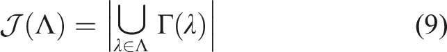
An iterative objective of DFR is to ensure maximum coverage of the current unknown space is maintained. ϒ supports evaluation of the coverage completeness of the unknown map space by the current views Λ. Let ${\mathcal{F}}^{cvr}$ represent the set of covered frontiers, where a frontier is considered covered if it has at least one covering view able to observe it according to ϒ. The residual set is represented as ${\mathcal{F}}^{\overline{cvr}}=\mathcal{F}\setminus {\mathcal{F}}^{cvr}$ , and the global coverage completeness is evaluated by the fraction of covered frontiers, ${\mathcal{F}}^{cvr}/\mathcal{F}$ . The iterative coverage maximization objective can be formulated as:

$\max \frac{\left|{\mathcal{F}}^{cvr}\right|}{\left|\mathcal{F}\right|}=\max \left|{\displaystyle \bigcup }_{f\in \mathcal{F}}\{f\mid \exists \lambda \in \mathrm{\Lambda },\text{Vis}({\mathit{m}}_f,\lambda )\}\right|.$

(11)

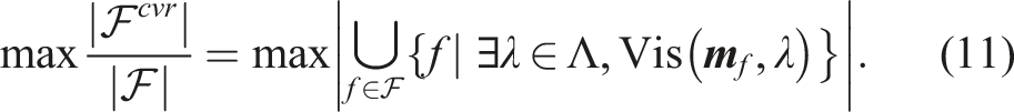
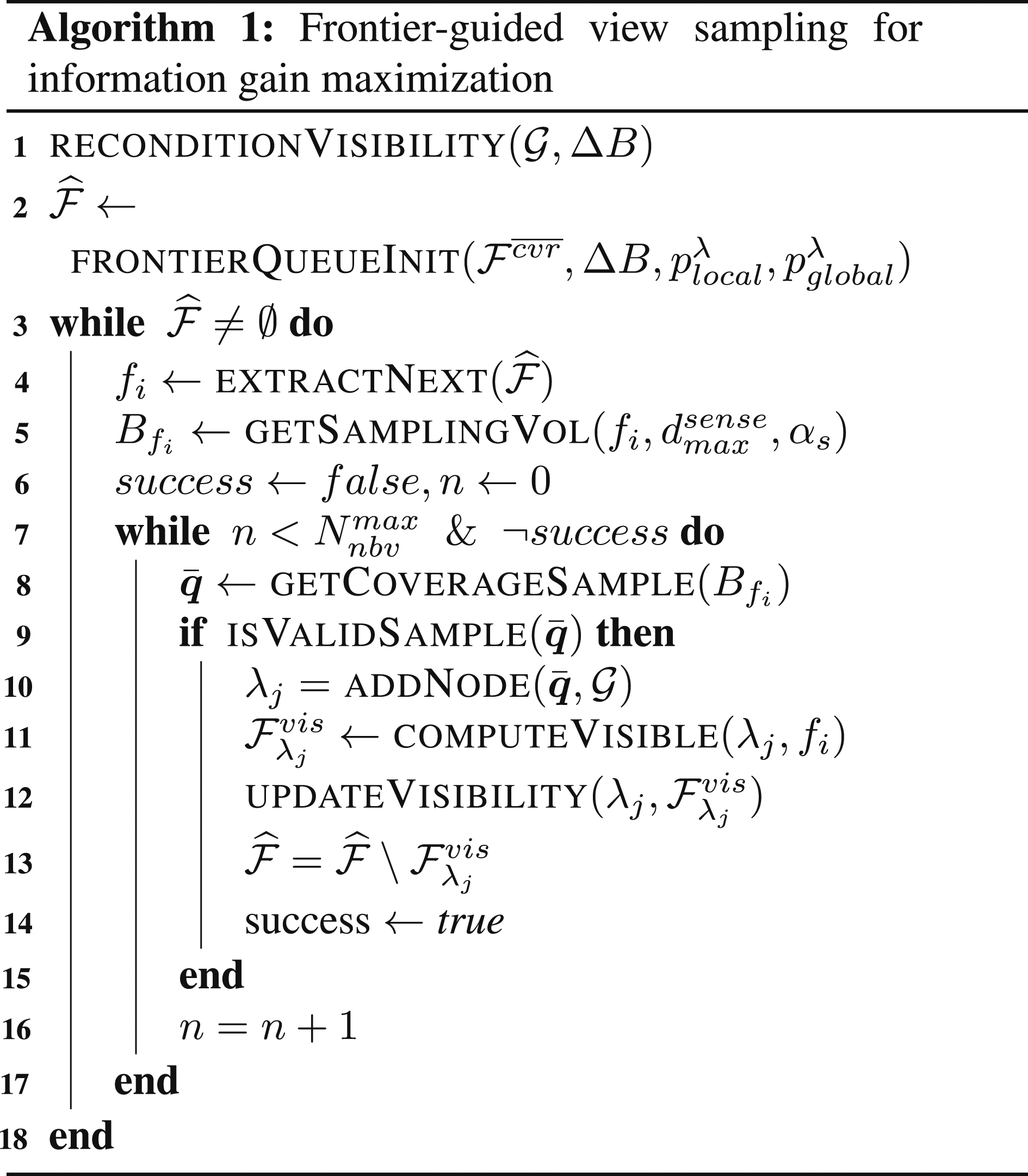
A frontier-guided sampling strategy is presented to perform the maximization of (11) by iteratively sampling viewposes to observe the non-covered frontiers. This effort is concentrated within ΔB which contains the most recent changes to the frontier distribution. Given the high complexity potentially involved in the sampling procedure, a performance tuning parameter $p_{local}^{\lambda }\in (0,1]$ is provided, representing a probability threshold used to select a random subset of the frontiers in ΔB to be considered for sampling in the current cycle.

A second parameter $p_{global}^{\lambda }\in (0,1]$ is provided which serves a similar purpose as $p_{local}^{\lambda }$ , but is applied to any non-covered frontiers that lie outside of ΔB. This is to account for possible frontiers that were not successfully covered in a finite number of attempts during previous DFR cycles, which can result when large amounts of occupied or unknown space exist near a frontier. The difficulty in finding a feasible viewpose can greatly increase for these cases, and in some cases one may not exist with the available map knowledge. Given the increased difficulty, $p_{global}^{\lambda }$ is given a lesser value than $p_{local}^{\lambda }$ , allowing the search effort to persist between DFR cycles but with lower priority. In effect, this offers a degree of probabilistic completeness as the likelihood of finding a valid sample, if one exists, can continually increase over time while reducing the individual search effort per DFR cycle.

The sampling procedure is given in Alg. 1, which begins by calling reconditionVisibility to update the visible information of existing views within the changed volume. Between cycles, the frontier boundaries are often pushed back by only a small amount, but remain visible within the many of the same view as the previous cycle. This step ensures these differences are updated, so sampling is only needed when frontiers are pushed beyond visibility of all existing views.

Next, a frontier queue $\widehat{\mathcal{F}}$ is initialized containing the selected subsets from ${\mathcal{F}}^{\overline{cvr}}$ . For each $f_i\in \widehat{\mathcal{F}}$ , a sampling subspace $B_{f_i}$ is computed from which f _i can potentially be observed given the sensing parameters. For a maximum of $N_{nbv}^{\mathit{max}}$ attempts, viewposes are randomly sampled using getCoverageSample and checked by isValidSample to determine if a valid sample has been found. A sample is considered valid only if it is collision-free and successfully observes the current frontier target, f _i .

Upon finding a valid sample, it is used to add a new node to the network, and all of its visible frontiers are computed to update the visibility map. If any of these frontiers are contained in $\widehat{\mathcal{F}}$ , they are removed since they have been already covered by the current sample. This can greatly reduce the number of samples, since in practice a single view will often be able to observe many nearby frontiers.

3.3.3. Pruning and refinement

The growth rate of the network is reduced by pruning unnecessary views that no longer provide any individual gain contribution, and redundant views with little or no exclusive information gain. These conditions naturally occur as the robot progresses its exploration of the map and observes the previously unknown space within each view. They also occur as a result when new view samples are added to the network which overlap with the pre-existing views, decreasing their exclusive gain. The goal is to identify the views that can be removed from the network without loss of the overall joint gain.

Given the initial views Λ and their joint gain $\mathcal{J}\left(\mathrm{\Lambda }\right)$ , pruning is defined by the objective of finding the minimum subset Λ* ⊂ Λ capable of producing the same gain measure, $\mathcal{J}(\mathrm{\Lambda }*)\equiv \mathcal{J}\left(\mathrm{\Lambda }\right)$ . This can be formulated as a submodularity maximization problem. Let σ _i be a Boolean indicator for each view in Λ, and let σ = {σ _i }, i = [0, ⋯|Λ|]. Let Λ _σ = {λ _i ∈ Λ∣σ _i = 1} be the subset of views dictated by σ . Let ${\mathcal{J}}_M\left({\mathrm{\Lambda }}_{\sigma }\right)$ represent the mutual information gain of σ , which refers to the common information covered by multiple views. The constrained optimization objective is then described as:

$\begin{array}{l}\mathit{\sigma }*=\mathrm{argmin}\left({\mathcal{J}}_M\left({\mathrm{\Lambda }}_{\mathit{\sigma }}\right)\right),\\ \mathbf{ }\mathbf{ }\mathbf{ }\mathbf{ }\mathbf{ }\mathbf{ }\mathbf{ }\mathbf{ }\mathbf{ }\mathbf{ }\mathbf{ }\mathbf{ }\mathbf{ }\mathit{\sigma }\\ \mathrm{s}.\mathrm{t}.\\ \mathcal{J}\left(\mathrm{\Lambda }\right)-\mathcal{J}\left({\mathrm{\Lambda }}_{\mathit{\sigma }}\right)=0,\end{array}$

(12)

where $\mathcal{J}\left(\mathrm{\Lambda }\right)-\mathcal{J}\left({\mathrm{\Lambda }}_{\mathit{\sigma }}\right)=0$ is a constraint applied to restrict the feasible subsets to those which do not decrease the joint gain achieved by the initial set.

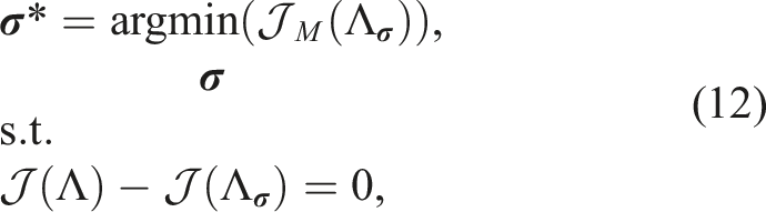
To solve Equation (12), a set of pruning candidates is found by searching for views that have negligible individual or exclusive information gain. Given the local difference neighborhood ΔB, the search is restricted to the views located within visible range $d_{\mathit{max}}^{sense}$ of ΔB, corresponding to the views with visibility information that was potentially effected by the map changes. The candidates within this region are further evaluated for their edge connectivity. Any candidate found to have a cut-edge is preserved to maintain the graph connectivity, while the remainder are deleted.

Once the pruning stage is complete, the coverage views of ${\mathcal{V}}^{nbv}$ represent the supremal set that maximizes map coverage using a minimal number of views. Not only does this help to reduce the total size, but the minimization of redundant coverage helps to simplify the planning problem. Since each NBV has some positive amount of exclusive gain after pruning, they represent an exact set of targets that a planner must determine how to optimally visit, without the need to evaluate their redundancy during its search.

3.3.4. Reachability update

The reachability knowledge represented by $\mathcal{E}$ is updated each iteration to account for new map knowledge and any state changes in $\mathcal{V}$ . Additional nodes are also sampled during this stage to increase the overall node density and uniformity in ${\mathcal{V}}^{\mathcal{X}}$ . This accounts for the non-uniformity of coverage view sampling, which is biased towards the frontier boundaries. Since the purpose of ${\mathcal{V}}^{\mathcal{X}}$ is primarily to increase the network connectivity, only the position of these samples is needed, while the visible information and pose orientation attributes can be ignored.

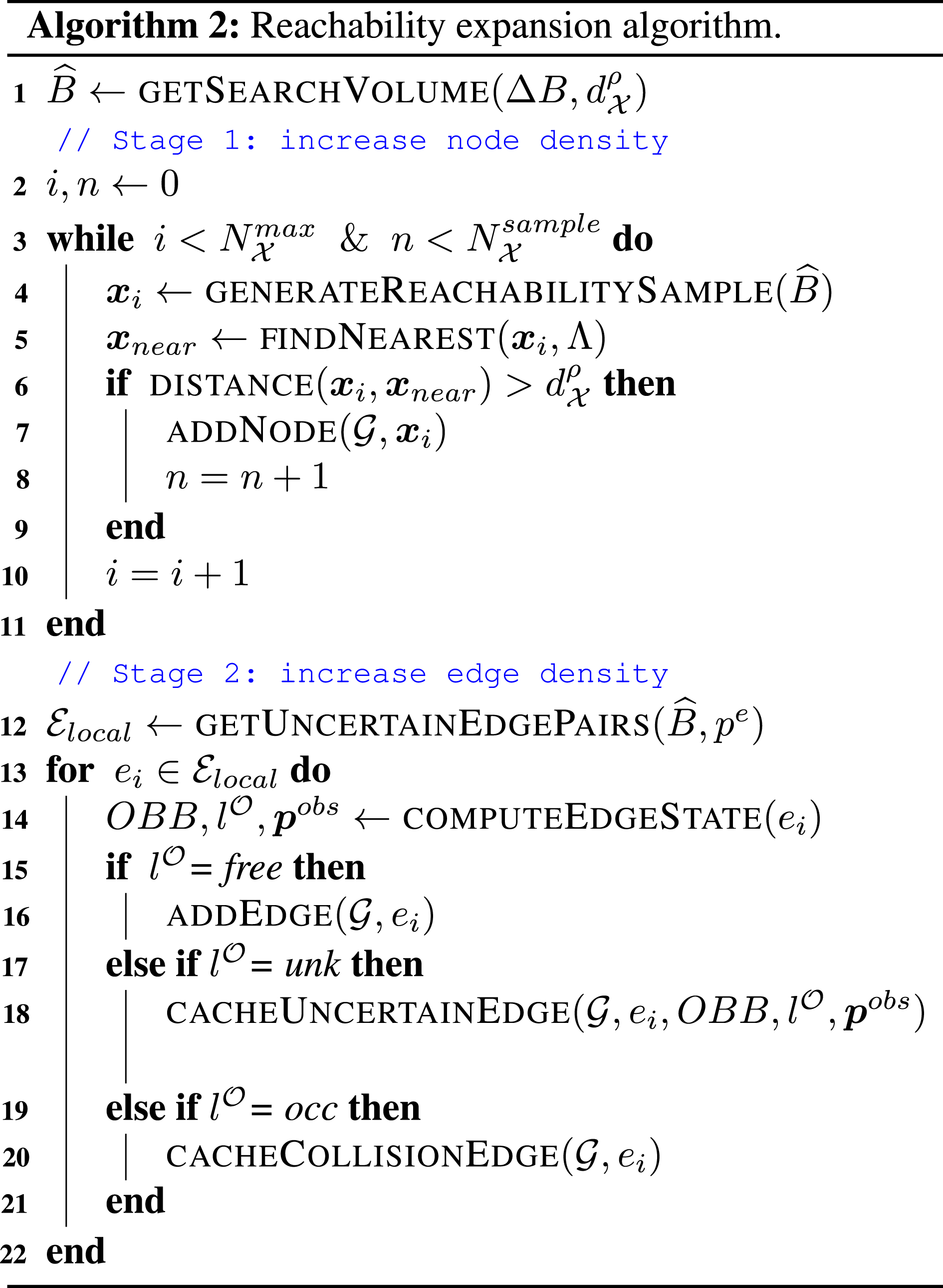
The pseudocode for the reachability update procedure is shown in Alg. 2, which contains two primary stages. The first stage samples traversal nodes to increase the distribution density within the graph, and the second stage increases the total edge density.

In the first stage, collision-free positions are uniformly sampled from $\widehat{B}$ , for a maximum of $N_{\mathcal{X}}^{\mathit{max}}$ attempts, or until a threshold of $N_{\mathcal{X}}^{sample}$ samples are accepted. Each sample is evaluated according to the distance of its nearest neighbor in Λ, and compared against a threshold distance, $d_{\mathcal{X}}^{\rho }$ . $d_{\mathcal{X}}^{\rho }$ serves as a density constraint to prevent too many samples from being added in close proximity, which would unnecessarily increase the size complexity of the graph while adding little or no additional reachability knowledge. A sample is accepted if its nearest neighbor distance is greater than $d_{\mathcal{X}}^{\rho }$ , and a new node is added to the graph using the sampled position.

The second stage begins by extracting the local set of candidate edge pairs ${\mathcal{E}}_{local}$ using the function getUnknownEdgePairs. This procedure searches $\widehat{B}$ to find the set of node pairs (v _u , v _w ) such that the collision state of the corresponding edge e_u,w is either null or unknown. Here, a null edge indicates the edge does not exist (i.e., has not been evaluated in any DFR cycle), while unknown refers to an edge found with an uncertain collision state from a previous DFR cycle. A parameter p ^e ∈ [0, 1) is used to specify a random probability threshold of whether to evaluate a candidate node pair (v _u , v _w ). This helps to limit the number of edge evaluation operations that occur per cycle, similar the parameter $p_{local}^{\lambda }$ used for coverage view sampling.

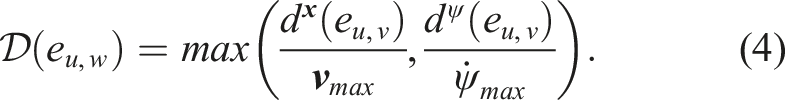
Each edge is evaluated by computeEdgeState to determine its collision state data, which leverages previously cached results if available. Since edges may be evaluated between any nodes over any distance within $\widehat{B}$ , the cached collision data can significantly reduce the update complexity. If an occupied collision is found, the edge is added to the cache of collision edges to prevent future evaluation. For unknown voxel collisions, the edge is added to the cache of uncertain edges along with the intermediate collision data results to accelerate future re-evaluation. Otherwise, the edge is added to the graph by addEdge which computes and stores its associated cost information according to (3) for efficient lookup by other procedures and planning.

3.3.5. Topological clustering

The graph nodes are decomposed into a set of subgraph regions represented by the hyperedges $\mathcal{C}$ , as illustrated in Figure 2(b). $\mathcal{C}$ serves as a topological hierarchy over $\mathcal{G}$ to reduce its size complexity. This representation can be utilized to increase the efficiency for search, traversal, and other operations. A tradeoff occurs where greater reductions in size complexity also result in reduced level of detail (LoD), that is, resolution.

Figure 2.

Depictions of the APN composition.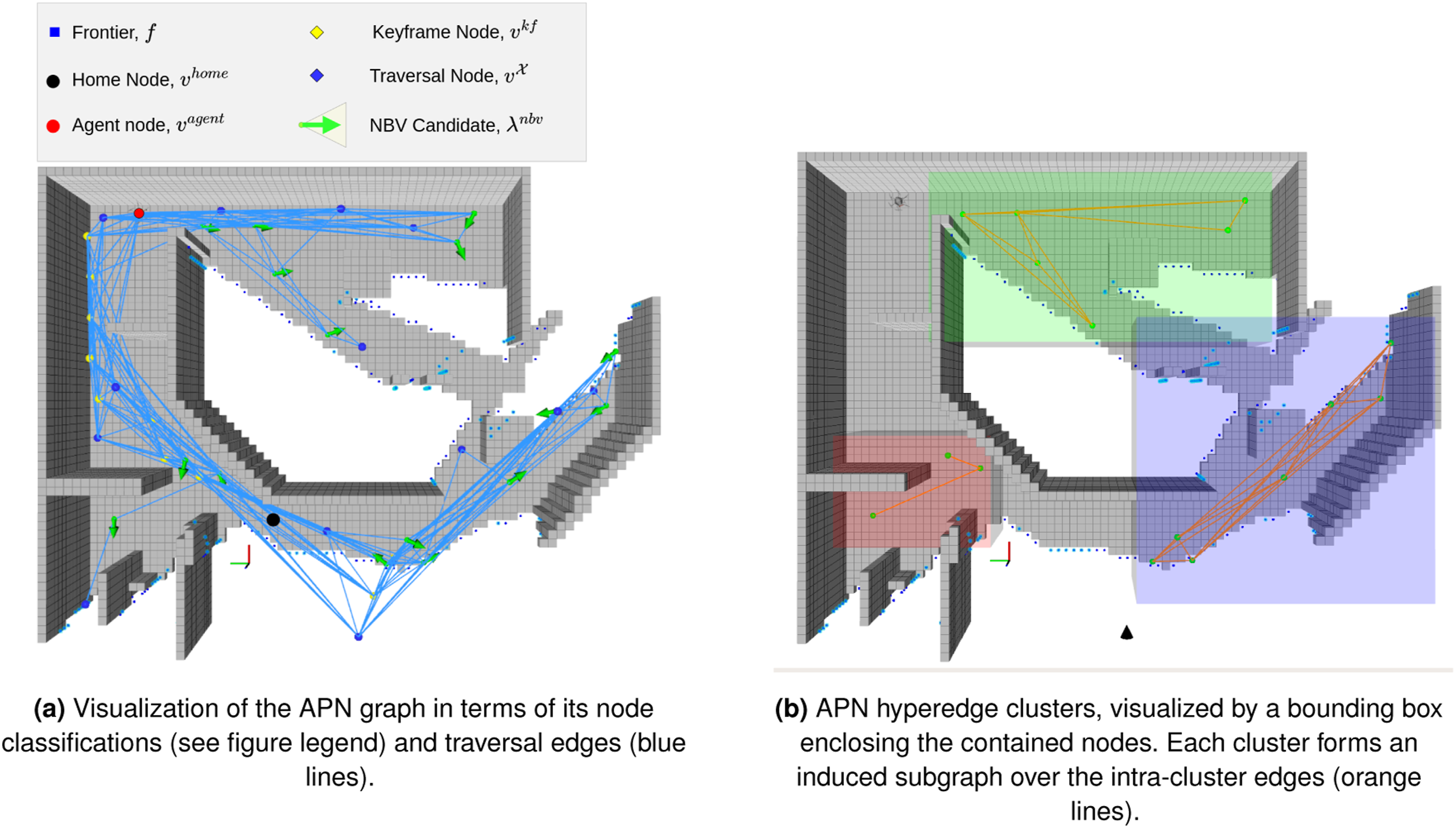

To compute the hyperedges, we use a density-based clustering approach based on Ankerst et al. (1999) and Ester et al. (1996), extended to leverage both the geometric and reachability knowledge already present in the APN. The algorithm uses two parameters, D _c and ρ _c , where D _c defines neighborhood distance threshold, and ρ _c defines a density threshold for the neighborhood.

Let a node v _p be defined as a core node if it has at least ρ _c edge-connected neighbors within distance D _c . A node v _q is then defined as a reachable node from v _p only if there exists an edge connection between v _p and v _q , and v _q is within distance D _c from v _p . Given a core node v _p , a cluster is formed by all nodes reachable from v _p . Any remaining nodes that are neither core nodes nor reachable from a core node are assigned as singleton clusters.

This approach allows clusters to form more naturally by additionally considering the edge connectivity between points. They are also not required to be geometrically convex as with other clustering approaches. This enables fewer clusters to be formed, since they can be better fit to the nodes over arbitrarily shaped space. Explicit constraints on the maximum number of clusters or their size are also not necessary, such that clusters can conform to the map with variable size and density, which can effectively handle environments where different regions may have different geometric characteristics and complexities.

3.4. Hierarchical evolutionary view planning

The iteratively updated APN provides a generalized representation of the exploration state space, which can be utilized by any graph-based planning strategy for global and local planning. In this section, we present an anytime planning approach referred to as the APN Planner (APN-P), which leverages the hierarchical decomposition of the APN to plan a global sequence over the topological subgraph regions. A second planning stage then optimizes the low-level view path for the first subgraph of the topological sequence. Each stage is formulated as a Fixed-Ended Open Traveling Salesman Problem (FEOTSP), solved using an evolutionary optimization approach to determine the optimal sequence orders. A visualization of this procedure is displayed in Figure 3.

Figure 3.

Visual depiction of the hierarchical planning strategy. The first stage computes the global path (dark red arrows) over the node clusters, with the start fixed to the robot location and the end fixed to the home location. The second stage optimizes the NBV sequence (depicted using tan arrows) within the first cluster of the global sequence (green bounding box).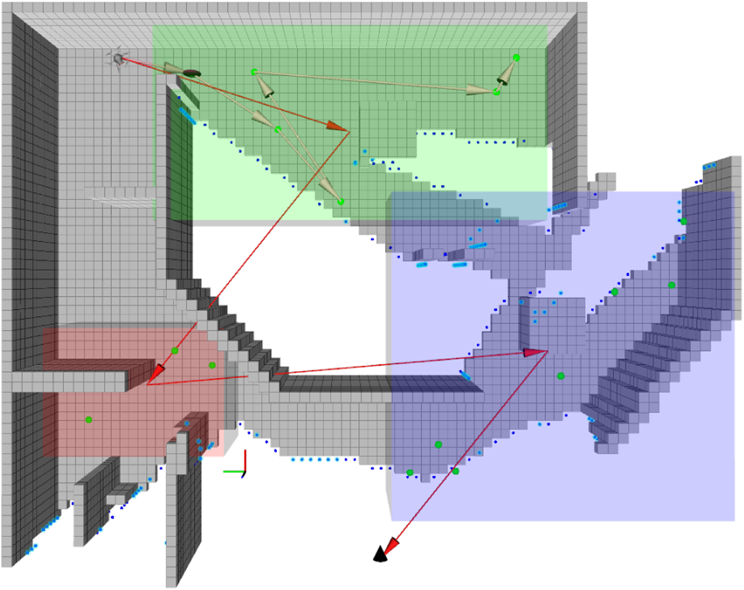

Let ${\mathbb{J}}^{\mathcal{H}}\mathbb{\subset }\mathbb{N}$ be an index set that enumerates the clusters $\mathcal{C}$ . A cost matrix ${\mathit{m}}^{\mathcal{H}}$ is computed by finding the shortest path between the centroid views of each pair of clusters. Given the pairwise cost $s\left(u,w\right)\in {\mathit{m}}^{\mathcal{H}}$ between cluster indices $u,w\in {\mathbb{J}}^{\mathcal{H}}$ , the cluster planning objective is to find the minimum cost permutation ${\mathrm{\Pi }}^{\mathcal{H}}\in {\mathit{S}}_n\left({\mathbb{J}}^{\mathcal{H}}\right)$ of the indices ${\mathbb{J}}^{\mathcal{H}}$ , where ${\mathit{S}}_n\left({\mathbb{J}}^{\mathcal{H}}\right)$ is the symmetric group of ${\mathbb{J}}^{\mathcal{H}}$ .

Given first cluster ${\mathcal{H}}_0$ of ${\mathrm{\Pi }}^{\mathcal{H}}$ , and its induced subgraph $\mathcal{G}\left[{\mathcal{H}}_0\right]$ , the view planning procedure is similarly formulated. Given an index set ${\mathbb{J}}^{\mathrm{\Lambda }}\mathbb{\subset }\mathbb{N}$ enumerating the NBVs $\left\{\lambda \right\}\in \mathcal{G}\left[{\mathcal{H}}_0\right]$ , a pairwise cost matrix m ^Λ between index pairs $u,w\in {\mathbb{J}}^{\mathrm{\Lambda }}$ can be obtained directly from the existing edge costs. The view path planning objective is then to find the minimum cost permutation ${\mathrm{\Pi }}^{\lambda }=\left(v^{agent},{\lambda }_{{{\mathbb{J}}^{\mathrm{\Lambda }}}_0},\dots ,{\lambda }_{{{\mathbb{J}}^{\mathrm{\Lambda }}}_n}\right)$ , which begins at the current robot configuration v ^agent and visits each NBV node of the target cluster.

The optimized sequences are preserved in a data cache allowing them to be used to re-initialize subsequent planning cycles. Given a planning cycle i and target cluster $\mathcal{G}\left[{\mathcal{H}}_0\right]$ , the current solution Π _i is initialized from Π_i−1 by first filtering out any invalid views ${\mathrm{\Pi }}_{i-1}\setminus \mathcal{G}\left[{\mathcal{H}}_0\right]$ that do not belong to the current cluster. The relative order over the common subset ${\mathrm{\Pi }}_{i-1}\cup \mathcal{G}\left[{\mathcal{H}}_0\right]$ is preserved, and any additional views $\mathcal{G}\left[{\mathcal{H}}_0\right]\setminus {\mathrm{\Pi }}_{i-1}$ are inserted using local search to estimate their optimal sequence positions.

Sequence optimization is executed using a mimetic evolutionary algorithm (Deb et al., 2002). Given the reference index set, $\mathbb{J}$ , a population of N _p candidate sequences are initialized by randomizing the permutation order of the reference indices. If a previous solution exists, the candidates are initialized by adding randomization to the previous solution. For a maximum of N _gen generations, the candidates are evolved by pairwise swapping element position to perform mutations, and using partially mapped crossover (PMX) (Kora and Yadlapalli, 2017). The procedure terminates once N _gen generations is exceeded, or an improved solution cannot be found after N _stall generations. Since solutions are initialized by those from the previous cycle, parts of the previous optimizations are carried over which helps increase the convergence rate of next cycles. This can increase the planning scalability as the size of the sequence candidates increases.

Once the exploration plan optimization is complete, the first view of the local sequence represents the updated navigation goal, λ _g . If the robot is not currently navigating towards a goal, or if the previous goal has already been reached, a trajectory is computed to reach λ _g by RRT* (Sucan et al., 2012), using the APN to find a feasible path to initialize the trajectory planner. Similarly, if the reward of current goal falls to zero and is pruned by the latest DFR update, the new λ _g is automatically set as the current target.

For cases where the robot is still navigating towards a previous goal λ_g,prev ≠ λ _g that has not yet been reached, the planner decides whether to reject λ _g until λ_g,prev ≠ λ _g is reached, or to immediately accept and begin navigation towards λ _g . This is decided by comparing the cost and rewards of their respective sequences, adding a penalty for changes to the direction of motion. In this way, the robot does not commit to a given goal until it is reached, but constantly evaluates if a better goal has been discovered. This is in contrast to many existing approaches, which often fully execute each goal before replanning.

3.5. Computational complexity

Occupancy queries require $\mathcal{O}\left(\log \left(\left|\mathcal{M}\right|\right)\right)$ using the octree-based representation in our implementation. From this, collision queries of a bounding sphere with safety radius d _safe take $\mathcal{O}\left(d_{safe}^3/r_{\mathcal{M}}\times \log \left(\left|\mathcal{M}\right|\right)\right)$ time, and edge queries between two points with distance d _e take $\mathcal{O}\left(d_e{d}_{safe}^2/r_{\mathcal{M}}\times \log \left(\left|\mathcal{M}\right|\right)\right)$ . Visibility queries operate by checking the occupancy values along a raycast, such that each raycast takes time $\mathcal{O}\left(d_{sense}/r_{\mathcal{M}}\times \log \left(\left|\mathcal{M}\right|\right)\right)$ given maximum sensor range d _sense .

The local change neighborhood ΔB is used to guide each DFR stage. Define $N^{\mathcal{F}}$ as the global number of frontiers in the map, with $N^{{\mathcal{F}}^{\overline{cvr}}}\le N^{\mathcal{F}}$ as the number of uncovered frontiers, and the respective fractions of these within ΔB is given as $N_{\mathcal{L}}^{\mathcal{F}}$ and $N_{\mathcal{L}}^{{\mathcal{F}}^{\overline{cvr}}}$ . The Visibility Update process recomputes the coverage status of each local frontier within the local region, resulting in $\mathcal{O}\left(N_{\mathcal{L}}^{{\mathcal{F}}^{\overline{cvr}}}\times \log \left(\left|\mathcal{M}\right|\right)\right)$ . For NBV Sampling, a maximum of $N_{nbv}^{\mathit{max}}$ attempts are permitted to find a valid sample for each uncovered frontier in the queue $\widehat{\mathcal{F}}$ , and size of $\widehat{\mathcal{F}}$ is constrained by the parameters $p_{local}^{\lambda }$ and $p_{global}^{\lambda }$ . Assuming a small value is used for $p_{global}^{\lambda }$ , the resulting complexity for NBV sampling is then $\mathcal{O}(p_{local}^{\lambda }\times N_{\mathcal{L}}^{{\mathcal{F}}^{\overline{cvr}}}$ $)$ .

For the Pruning stage, evaluating pruning conditions for each view can be done in constant time, and each view contained by ΔB is checked to yield a complexity $\mathcal{O}\left(\left|{\mathrm{\Lambda }}_{\mathcal{L}}^{nbv}\right|\right)$ , where ${\mathrm{\Lambda }}_{\mathcal{L}}^{nbv}\subseteq {\mathrm{\Lambda }}^{nbv}$ is the subset of NBVs within ΔB. Similarly, Traversal Sampling and Edge Analysis operate only on the elements contained by ΔB. Given that $d_{\mathcal{X}}^{\rho }$ defines the minimum spacing distance between sampled configurations, the number of possible nodes within the local volume will be proportional to $\left(\left|\mathrm{\Delta }B\right|/d_{\mathcal{X}}^{\rho }\right)$ . The Clustering stage then operates on the resulting NBVs after being processed by the previous stages with complexity $\mathcal{O}\left(\left|{\mathcal{V}}^{nbv}\right|\times \log \left(\left|{\mathcal{V}}^{nbv}\right|\right)\right)$ based on (Ankerst et al., 1999).

The complexity of planning depends primarily on the construction of the cost matrix, and the sequence optimization. Edge costs can be retrieved from the APN in constant time for adjacent nodes, but otherwise require path search using A* (or similar algorithms), which takes $\mathcal{O}\left(\left(\left|\mathcal{E}\right|+\left|\mathcal{V}\right|\right)\times \log \left(\left|\mathcal{E}\right|\right)\right)$ per path. Sequence optimization uses the NSGA-II algorithm Deb et al. (2002), which has complexity $\mathcal{O}\left(N_p^2\right)$ , and the evolutionary optimization given maximum generations N _gen is $\mathcal{O}\left(N_{gen}\times N_p^2\times \left|{\mathcal{V}}^{nbv}\right|\right)$ .

A summary of the key complexity analysis terms is provided in Table 1. The complexity of the DFR stages can be constrained by a constant factor on the size of the local change volume, independent of the total size of the map or APN. The user-defined parameters provide an added level of control over the amount of data processed per cycle, allowing each cycle to compute faster. This allows the effort to be distributed over multiple cycles by processing only a random subset per cycle, rather than expending the maximum effort on every cycle. Empirical testing has indicated they can be useful for fine-level optimization if desired or if certain knowledge of the environments characteristics are available, but precise tuning is not critical to feasible operation.

Table 1.

Summary of Computational Complexity Terms.

Operation	Complexity
Visibility Update	$\mathcal{O}\left(N_{\mathcal{L}}^{{\mathcal{F}}^{\overline{cvr}}}\times \log \left(\left|\mathcal{M}\right|\right)\right)$
NBV Sampling	$\mathcal{O}\left(p_{local}^{\lambda }\times N_{\mathcal{L}}^{{\mathcal{F}}^{\overline{cvr}}}\times \log \left(\left|\mathcal{M}\right|\right)\right)$
Pruning	$\mathcal{O}\left(\left|{\mathrm{\Lambda }}_{\mathcal{L}}^{nbv}\right|\right)$
Traversal Sampling	$\mathcal{O}\left(N_{\mathcal{X}}^{\mathit{max}}\times \log \left(\left|\mathcal{M}\right|\right)\right)$
Edge analysis	$\mathcal{O}\left(\left(p^e\mathrm{\Delta }B/d_{\mathcal{X}}^{\rho }\right)\times {\left|\mathrm{\Lambda }\right|}^2\times \log \left(\left|\mathcal{M}\right|\right)\right)$
Clustering	$\mathcal{O}\left(\left|{\mathcal{V}}^{nbv}\right|\times \log \left(\left|{\mathcal{V}}^{nbv}\right|\right)\right)$
Plan Cost Matrix	$\mathcal{O}\left({\left|\mathrm{\Pi }\right|}^2\times \left(\left|\mathcal{E}\right|+\left|\mathrm{\Lambda }\right|\right)\times \log \left(\left|\mathcal{E}\right|\right)\right)$
Seq. Optimization	$\mathcal{O}\left(N_{gen}\times N_p^2\times \left|\mathrm{\Pi }\right|\right)$

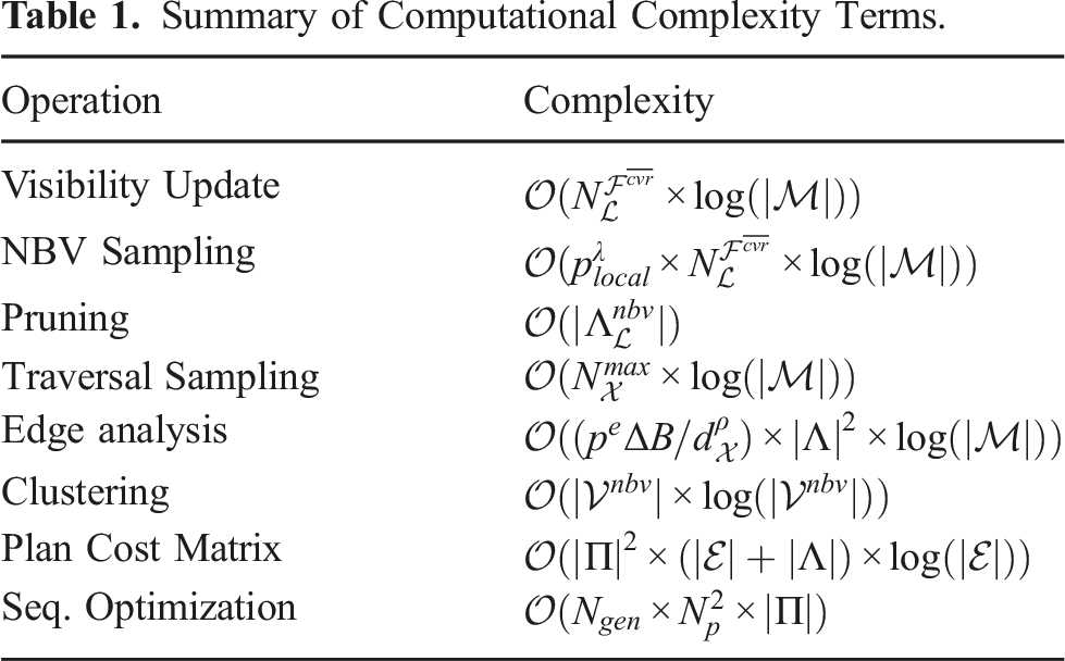
A significant component of the planning complexity is the construction of the cost matrix, which scales polynomial with the number of sequence elements (i.e., clusters and NBVs). Additionally, if elements are not directly adjacent, their cost must be computed by finding the shortest path through the graph. As the map is explored, the separation distance between many NBVs can continually increase, requiring larger search efforts through the graph. The cluster hypergraph helps reduce both the number of occurrences and cost of these long-distance path searches. Since each NBV polynomially increases the planning problem size, the Pruning Stage further helps to reduce the planning costs by ensuring only the minimal set of NBVs are included.

Finally, the running time is an important aspect that is generally hidden from the Big O notation, but is a critical factor for online algorithms. For example, an increase by a constant factor to the running time would not change its order of complexity, but the increased computation time would impact the online feasibility. The running time can have a direct impact on the overall exploration quality, since the optimality of a previously computed goal may decrease with new information. Faster update cycles help to minimize the time spent following inefficient paths as better ones become feasible. Our use of change detection and caching techniques helps to minimize the scale of each update and reduce wasteful or redundant computations, maximizing the rate of DFR and APN-P updates. The APEXMAP software framework additionally provides efficient data structures and design patterns for efficient management of dynamically changing data structures and other general runtime optimizations.

4. Evaluation

The APN and APN-P were evaluated through ROS-based simulations using Gazebo (Koenig and Howard, 2004) and the RotorS MAV simulation framework (Furrer et al., 2016). The AscTec Firefly MAV model provided by RotorS was used to simulate the robot dynamics and control systems, and was equipped with a stereo depth sensor for visual perception. The simulations and all algorithms were executed using a single laptop computer with Intel Core i7 2.6 GHz processor and 16 GB RAM. The test results were used to analyze the computational performance and planning efficiency of the proposed approach.

Exploration was tested using several different 3D structure models with various scales as displayed in Figure 4, with a visual comparison of their relative scales shown in Figure 4(e). In addition to varying sizes, each environment provides different characteristics for evaluation, such as obstacle density, narrow spaces opposed to open space, dead-ends, and overall geometric complexity.

Figure 4.

Visualization of each evaluated world scenario. The relative scale of each scenario is depicted in 4e according to their bounding box dimensions, where red represents the Apartment (slightly offset from the origin for visual clarity), blue represents the Maze, grey represents the Industrial Plant, and green represents the Warehouse.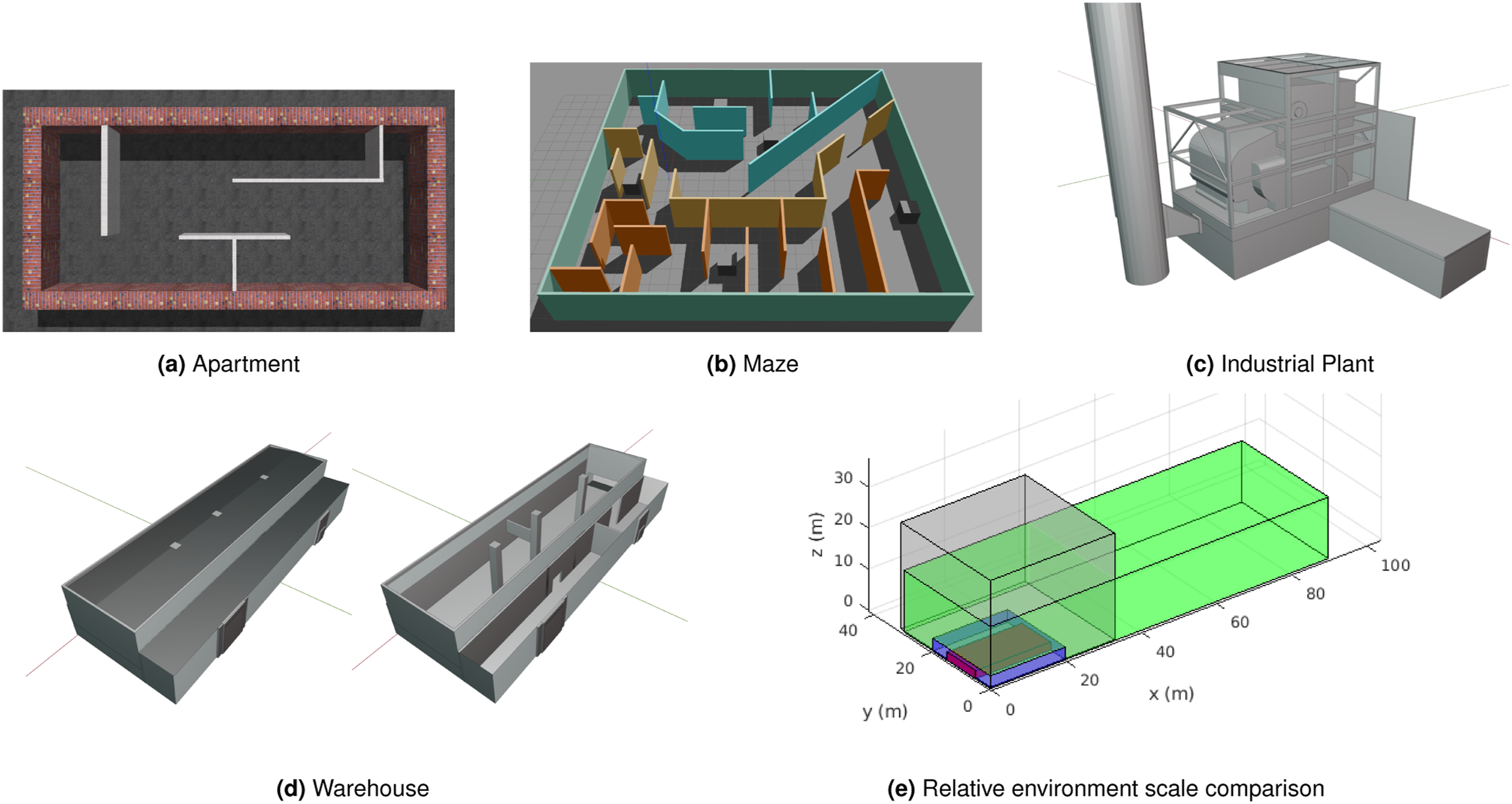

A video presentation demonstrating the operation and performance of the APN-P is included with this work. The simulation environment is used to visualize the concepts of operation as they are executed. The Apartment scenario is used in the video presentation to demonstrate the real-time operation of the full exploration procedure while visualizing the APN’s dynamically changing structure.

To account for the stochastic nature of the approach, each scenario was run five times and statistical analysis was computed over a variety of performance metrics, summarized in Table 2. The average total exploration runtime required to complete the exploration task is denoted as $\overline{T}$ , and ${\overline{t}}^{cycle}$ refers to the average computational time required per update and planning cycle. A maximum exploration time limit of T _max = 14min (840s) was imposed, which is the maximum rated flight time for the AscTec Firefly. If this threshold is exceeded, exploration immediately terminates and failure is reported.

Table 2.

Summary of Performance Analysis Metrics.

Symbol	Description
$\overline{T}$	Average total exploration runtime (s)
${\overline{t}}^{cycle}$	Average computational time per cycle (ms)
${\vartheta }_{\mathcal{M}}$	Final map surface coverage ratio (%) as ${\mathcal{M}}^{occ}/{\widehat{\mathcal{M}}}^{occ}$
${\eta }_{\mathcal{M}}$	Average voxel discovery rate (m3/s)
${\eta }_{{\mathcal{M}}^{occ}}$	Average surface voxel discovery rate (m3/s)
${\vartheta }_{\mathcal{V}}$	Avg. number of nodes per unit of map volume (1/100 m3)
${\vartheta }_{\mathcal{E}}$	Avg. ratio of known edges $\left|\mathcal{E}\right|$ to possible edges $\left(\begin{array}{l}\left|\mathcal{V}\right|\\ 2\end{array}\right)$

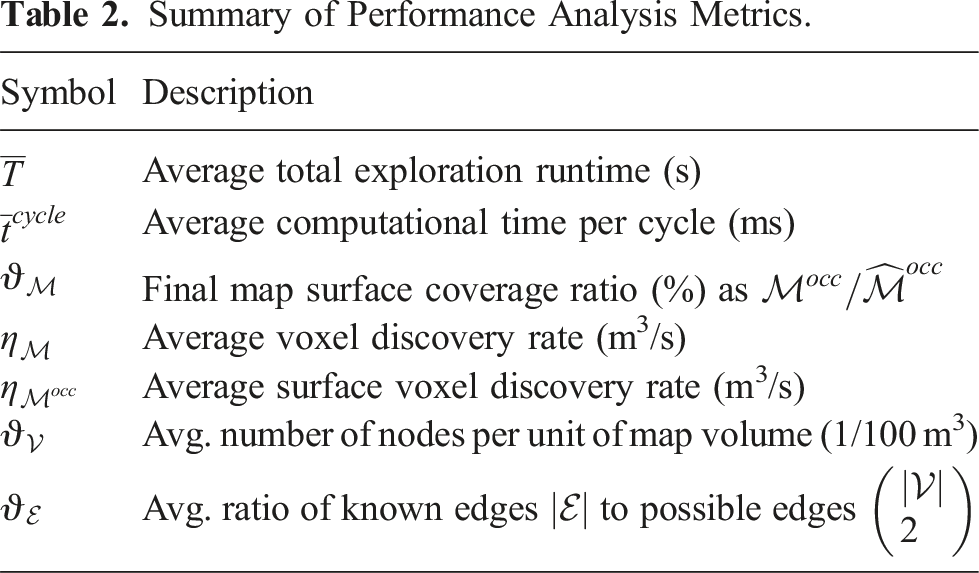
The total map coverage is given as the ratio ${\vartheta }_{\mathcal{M}}$ of the number of surface voxels ${\mathcal{M}}^{occ}$ discovered during exploration with respect to a ground truth set ${\widehat{\mathcal{M}}}^{occ}$ of all visible surface voxels. ${\widehat{\mathcal{M}}}^{occ}$ was determined by manually guiding the robot through each world scenario, carefully ensuring every observable surface was covered by the sensor. The total volumetric exploration rate is given as ${\eta }_{\mathcal{M}}$ , which is the average volume of new information gain per second in m³/s. Since the objective is to achieve complete surface coverage, a more useful metric is ${\eta }_{{\mathcal{M}}^{occ}}$ which refers to the rate of occupied information gain in m³/s.

The APN is evaluated according to its average node density ${\vartheta }_{\mathcal{V}}$ and edge density ${\vartheta }_{\mathcal{E}}$ . Here, node density refers to the number of nodes within a standard unit of volume, normalized as the number of nodes per 100 m³ of the mapped free space. Edge density refers to the ratio between the known edges $\left|\mathcal{E}\right|$ and the total edge capacity of a complete edge set over the nodes, $\left(\begin{array}{l}\left|\mathcal{V}\right|\\ 2\end{array}\right)$ . ${\vartheta }_{\mathcal{V}}$ and ${\vartheta }_{\mathcal{E}}$ are given as the average over all cycles of the test scenario.

The following baseline approaches were used for comparative analysis with the APN-P:

• RH-NBVP (Bircher et al., 2018): A receding horizon method that finds informative view paths using RRT-based expansion within a local region of the robot.

• AEP (Selin et al., 2019): An approach that extends the strategy of RH-NBVP, using RH-NBVP for local planning and frontier-based planning for global search when local planning fails to find informative views.

• FFI (Dai et al., 2020): A hybrid frontier-based and sampling-based approach that uses an efficient frontier clustering strategy to guide the sampling of views.

• Rapid (Cieslewski et al., 2017): An extension of frontier-based planning designed to maintain the fastest allowable velocity by guiding towards frontiers within the sensors current field of view, and using classical frontier planning when no visible frontiers are available.

A summary of common parameters for the different scenarios is shown in Table 3, which were selected as consistently as possible to the baseline approaches. The map resolution $r_{\mathcal{M}}$ was varied between the values {0.1, 0.2, 0.4}m to analyze its effects on performance scalability. The maximum linear velocity v _max and yaw rate ${\stackrel{.}{\psi }}_{\mathit{max}}$ were assigned based on the common values used in the comparative approaches, along with the sensing parameters $d_{\mathit{max}}^{sense}$ and (α _v , α _h ).

Table 3.

Summary of Common Configuration Parameters.

Param	Scenario
	Apt.	Maze	Ind. Plant	Warehouse
$r_{\mathcal{M}}$	{0.1, 0.2, 0.4}	{0.1, 0.2}	{0.2}	{0.4}
d safe	0.75m
v max	1.0 m/s	2.0 m/s	2.5 m/s	3.0 m/s
${\stackrel{.}{\psi }}_{\mathit{max}}$	0.75 rad/s
$d_{\mathit{max}}^{sense}$	5m	6m	7m	9m
α v , α h	[60°, 90°]	[60°, 90°]	[75◦, 115◦]	[75◦, 115◦]

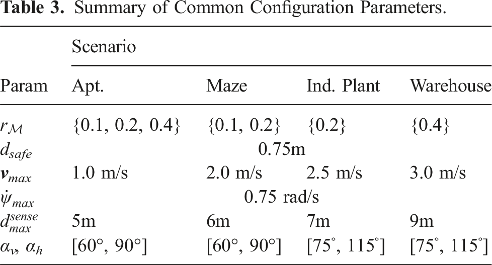
Coverage view sampling parameters related to Alg. 1 were set as $p_{local}^{\lambda }=0.8$ , $p_{global}^{\lambda }=0.1$ , and $N_{nbv}^{\mathit{max}}=30$ for each scenario. The reachability update parameters for Alg. 2 for each scenario were commonly set to $N_{\mathcal{X}}^{sample}=3$ , p ^e = 0.7, and $d_{\mathcal{X}}^{\rho }=2.0\mathrm{m}$ .

4.1. Apartment scenario

The apartment scenario in Figure 4(a) is a relatively small scale interior space with the dimensions 20 × 10 × 3(m³), used as a baseline for comparing the larger and more complex scenarios. An example map reconstruction by APN-P is shown in Figure 5(a) with the traced exploration path, and the APN roadmap is shown in Figure 5(b). The average distance traveled was 76.5 m, and a surface coverage completeness of ${\vartheta }_{\mathcal{M}}=100\%$ was consistently achieved at each evaluated map resolution.

Figure 5.

Exploration results for the Maze Scenario. (a): The explored path is plotted in red, with intermediate keyframe configurations represented by yellow points. (b): The APN nodes and edges overlayed in blue.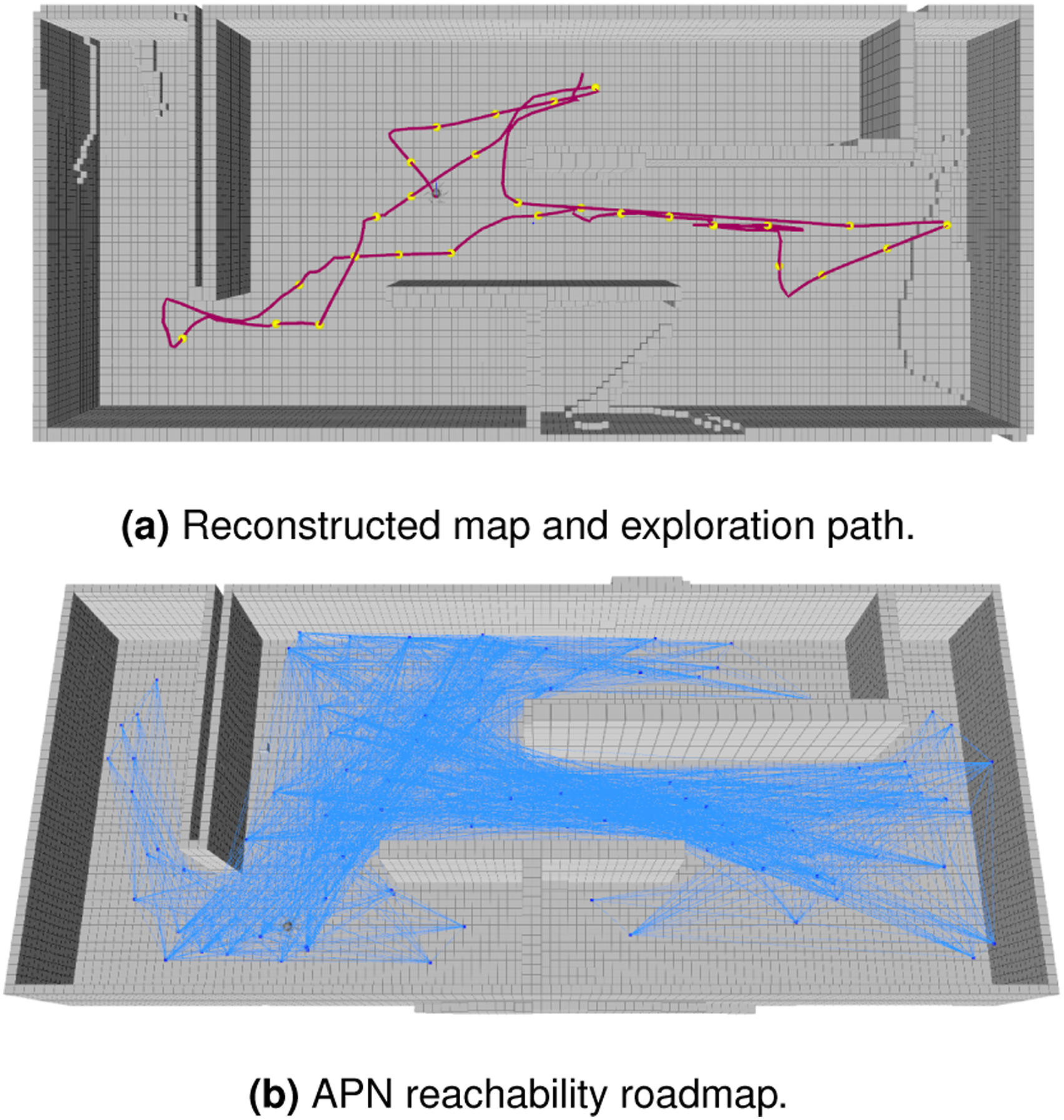

Figure 6(a) shows an example of the explored map volume over time using resolution 0.2 m for reference. The surface coverage rate ${\eta }_{{\mathcal{M}}^{occ}}$ was 1.5 m³/s and 2.6 m³/s for the respective map resolutions of 0.1 m and 0.2 m. Since there are multiple dead-end regions for this scenario, some amount of backtracking is unavoidable, where the effects of backtracking correspond to the periods in Figure 6(a) where the map growth briefly stagnates (e.g., around the 30s timestamp).

Figure 6.

Representative results of the exploration progress over time. (a) - (d): explored map in terms of total voxels and their volume. (e) - (h): corresponding APN size in terms of its nodes (red) and edges (blue), with the respective node density 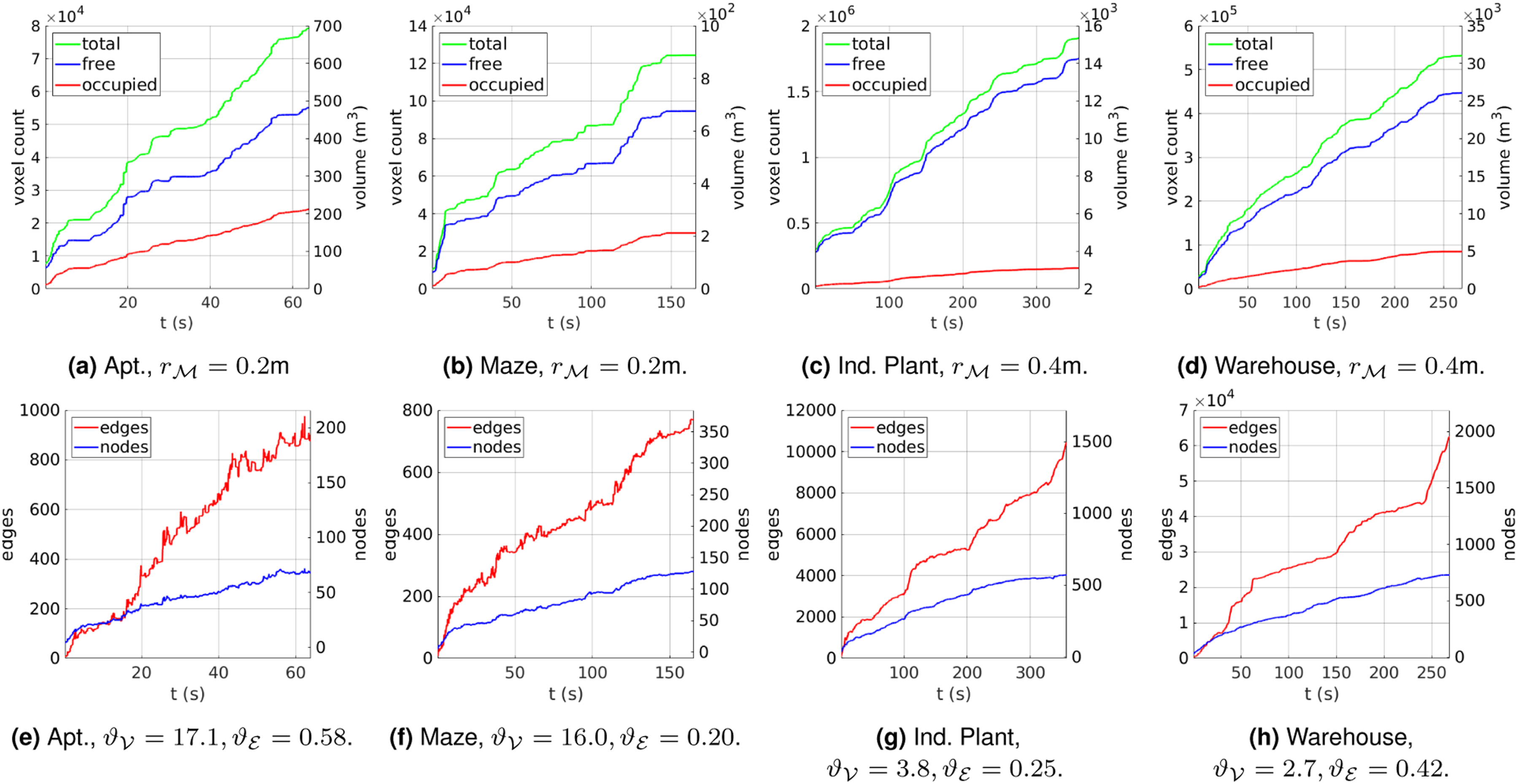$\left({\vartheta }_{\mathcal{V}}\right)$ and edge density $\left({\vartheta }_{\mathcal{E}}\right)$ .

The size growth of the APN over time is shown in Figure 6(e). Compared to the map scale in Figure 6(a), the APN is significantly smaller and its growth over time is non-monotonic due to iterative pruning and refinements. The final state of the APN roadmap is shown in Figure 5(b), which can be seen to expand throughout the reachable free-space at a sufficient density for planning and navigation.

Figure 7(a) shows representative results of the computation times per cycle, using map resolution 0.2 m as reference. The time taken for DFR remains fairly consistent over time despite the increasing map size. This demonstrates the effectiveness of the difference-aware update procedures at constraining the complexity as the map grows. A statistical boxplot of the respective procedures executed per cycle is shown in Figure 7(e). The majority of computation time per cycle was spent on view planning, which had a median value of 13.6 ms. The time spent on global cluster planning was negligible due to the relatively small size and complexity of this environment. The APN contained an average of only 1.2 clusters, resulting in a trivial instance of cluster sequence optimization. The computation times for all differential regulation procedures were minimal compared to planning, given the relatively simple environment.

Figure 7.

Timing performance for each exploration scenario. (a)–(d): depict the processing time taken per cycle. (e)–(h): display the median statistical boxplot of the DFR and planning computation times per cycle.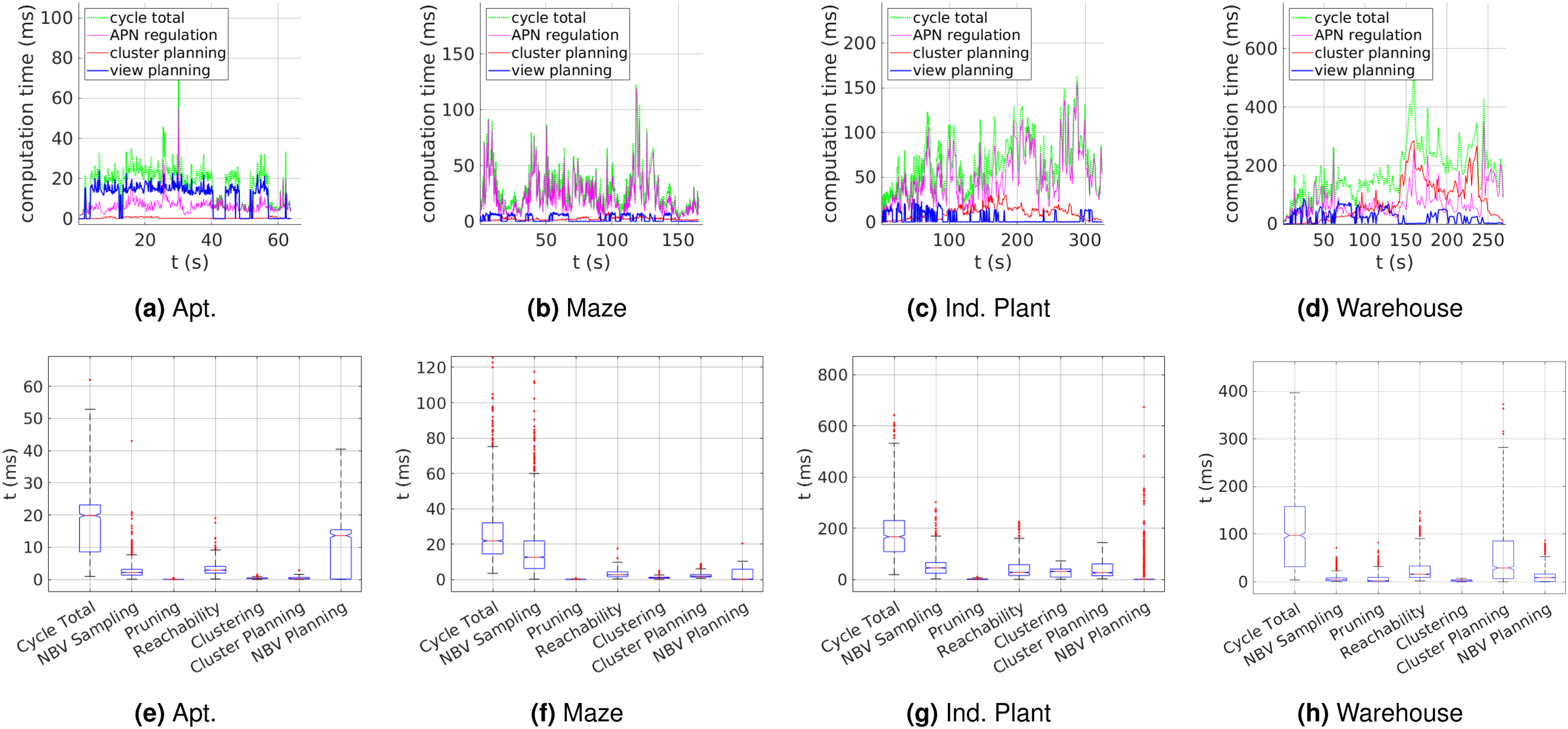

The time performance with the compared methods is summarized in Table 4. At the lowest map resolution of 0.4 m, the APN-P achieved an average total exploration time of $\overline{T}=52.9\mathrm{s}\pm 4.3\mathrm{s}$ , and average computation time per iteration of ${\overline{t}}^{cycle}=14.0\pm 8.0\text{ms}$ . Using a map resolution of 0.2 m, the average exploration time was 57.9s with 18.9 ± 9.1 ms per cycle. At the highest map resolution of 0.1 m, the average exploration time was 69.4s with average 28.9 ± 18.5 ms per cycle.

Table 4.

Time Performance Comparison in Terms of Total Exploration Completion Time $\overline{T}$ and Computation Time per Cycle ${\overline{t}}^{cycle}$ , Averaged Over Five Runs.

		APN-P		FFI		AEP		RH-NBVP		Rapid
Scenario	$r_{\mathcal{M}}\left[\mathrm{m}\right]$	$\overline{T}\left[\mathrm{s}\right]$	${\overline{t}}^{cycle}\left[\text{ms}\right]$	$\overline{T}\left[\mathrm{s}\right]$	${\overline{t}}^{cycle}\left[\text{ms}\right]$	$\overline{T}\left[\mathrm{s}\right]$	${\overline{t}}^{cycle}\left[\text{ms}\right]$	$\overline{T}$ [s]	${\overline{t}}^{cycle}\left[\text{ms}\right]$	$\overline{T}$ [s]	${\overline{t}}^{cycle}\left[\text{ms}\right]$
Apt.	0.4	52.9 ± 2.7	14.0 ± 8.0	80	122 ± 36	200	92	501.9	153	-	-
	0.2	57.9 ± 5.5	18.9 ± 9.1	-	156 ± 109	200	-	-	-	-	-
	0.1	69.4 ± 9.2	28.9 ± 18.5	151	68 ± 27	200	129	-	-	-	-
Maze	0.2	145.1 ± 11.7	26.1 ± 20.8	177	155 ± 71	-	-	-	-	-	-
	0.1	212.6 ± 18.9	48.0 ± 28.8	330	238 ± 80	-	-	-	-	-	-
Ind. Plant	0.2	353.1 ± 44.7	186.8 ± 113.4	>1000	152 ± 20	941	−	2104	−	582	−
Warehouse	0.4	268.1 ± 24.1	121.3 ± 84.4	-	-	-	-	-	-	-	-

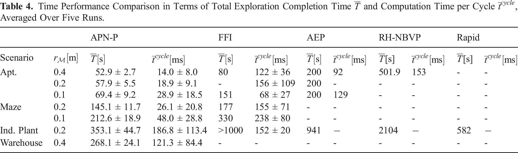
The RH-NBV approach required the highest total exploration time of 501.9s, with an average computation time per iteration of 153 ms. For AEP, the total exploration time for each resolution was reported to take approximately 200s on average (exact quantities were not specified), with an average computation time per iteration of 98 ms. FFI reported the fastest exploration time of the compared methods, with a total time of 80s and 151s for the respective map resolutions 0.4 m and 0.1 m. It should be noted that this approach was terminated once 95% exploration was reached, rather than full coverage.

The APN-P performance demonstrated a significant improvement over the compared state-of-the-art implementations in terms of both total exploration time and per-iteration computation times. Compared to FFI, APN-P achieved complete coverage while the exploration time was reduced by 34% using resolution 0.4 m, and 54% using resolution 0.1 m. Additionally, the percent improvement between resolutions indicates better scalability to higher resolution mapping.

4.2. Maze-like scenario

A maze-like environment is presented in Figure 4(b) with the dimensions of 20 × 20 × 2.5(m³). This scenario was tested using map resolutions of 0.1 m and 0.2 m; higher resolutions were not evaluated since there are narrow passageways that require lower resolutions to admit collision-free paths, as also noted in (Dai et al., 2020). This scenario was primarily compared against FFI, as this scenario was not evaluated in the original works of the other approaches.

A representative example of the mapped environment after exploration is shown in Figure 8(a) with the executed exploration path overlayed in red. The path shows that very few redundant motions were executed and progresses smoothly throughout the maze passages, with an average total path length of 208.9 m.

Figure 8.

Exploration results for the Maze Scenario. (a): The explored path is plotted in red, with intermediate keyframe configurations represented by yellow points. (b): The APN nodes and edges overlayed in blue.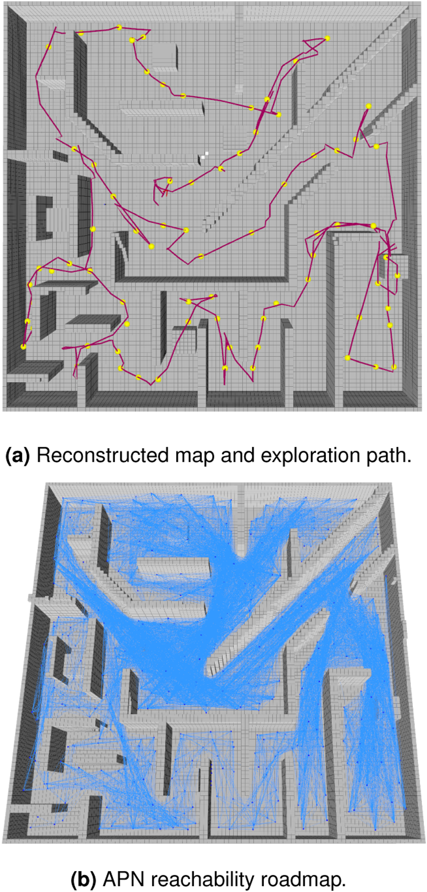

Figure 6(b) shows the map construction over time. An average coverage value of ${\vartheta }_{\mathcal{M}}=100\%$ was reached at each map resolution, and the surface coverage rate ${\eta }_{{\mathcal{M}}^{occ}}$ was 0.5 m³/s and 1.4 m³/s for the respective map resolutions of 0.1 m and 0.2 m. The APN size growth over time was plotted in Figure 6(f) and visualized in Figure 8(b). The average node density per 100 m³ was ${\vartheta }_{\mathcal{V}}=16.0\pm 1.3$ , with an average edge density of ${\vartheta }_{\mathcal{E}}=0.20\pm 0.12$ .

The computation times per cycle are plotted in Figure 7(b) with a statistical analysis of the computation time taken per procedure shown in Figure 7(f). For this scenario, most of the computation time went towards APN regulation, with coverage view sampling requiring the most time of 15.8 ms due to the prevalence of obstacles and occlusions. Despite the high obstacle density, the computation times for reachability updates remained relatively small, while still maintaining sufficient node and edge densities to facilitate planning. This demonstrates the effectiveness of the local difference-awareness and efficient data caching strategies that minimize wasteful or redundant processing.

Table 4 summarizes the exploration efficiency of the compared approaches with respect to total exploration time and computation time per cycle. Note that as previously mentioned, exploration time for FFI was reported when 95% coverage was achieved, rather than 100%. The APN-P completed the exploration with 100% coverage in an average time of 145.1s and 212.6s for map resolutions 0.2 m and 0.1 m, respectively. These are significant improvements over the results of FFI, while the processing time per cycle was also reduced by around 80% and had much less variability. Additionally, the total exploration time for FFI increased by 86% between the two map resolutions, while the respective increase for the APN-P was 45%. This further demonstrates the performance scalability for higher mapping resolutions using larger and more complex environments.

4.3. Industrial plant scenario

The Industrial Plant scenario shown in Figure 4(c) is an outdoor environment based on the Gazebo Powerplant model, truncated to the approximate dimensions of 33 × 31 × 26(m³). It represents both a large-scale and complex exploration task due to intricate structural geometries with many auto-occlusions. It was tested using a map resolution of 0.2 m and maximum velocity of 2.5 m/s, consistent with the compared approaches.

An example of the explored map is shown in Figure 9(a), with the explored volume over time plotted in Figure 6(c). A high surface coverage rate of ${\eta }_{{\mathcal{M}}^{occ}}=3.2{\mathrm{m}}^3/\mathrm{s}$ was achieved, which was consistently maintained as shown in Figure 6(c). The average total coverage was 98.7%, due to a few small regions with high surrounding occlusions, where coverage sampling failed to find a feasible viewpose. This could be overcome by selecting more aggressive sampling parameters, which was not done for these tests for parameter consistency between scenarios.

Figure 9.

Exploration results of the Industrial Plant scenario.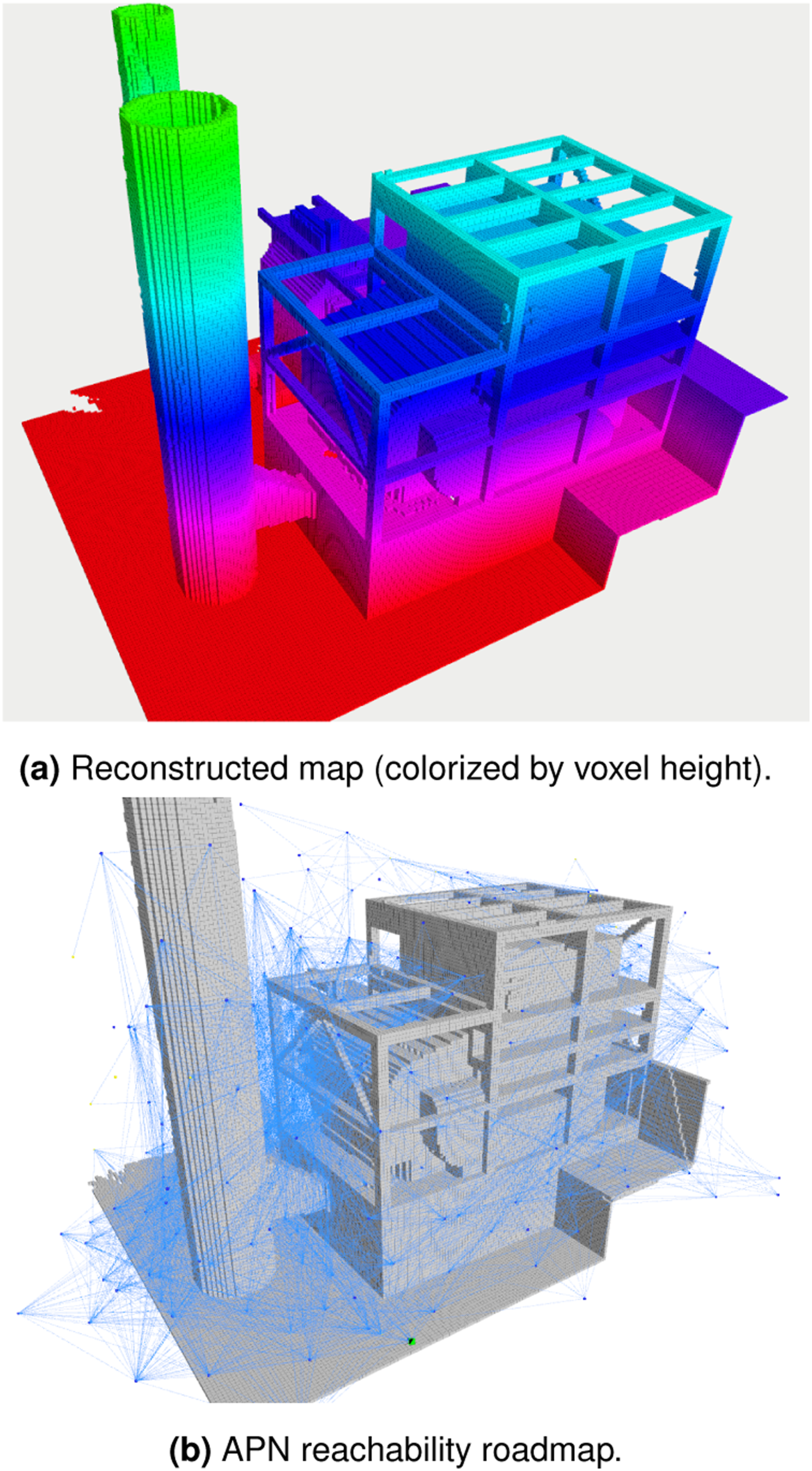

The APN size over time is plotted in Figure 6(g), with the final roadmap structure visualized in Figure 9(b). The average node and edge density were ${\vartheta }_{\mathcal{V}}=3.8$ and ${\vartheta }_{\mathcal{E}}=0.25$ , respectively. By visual inspection of Figure 9(b), the extent and density of the network appear to provide good coverage throughout the map.

The processing time per cycle is displayed in Figure 7(c), with a statistical boxplot of the time taken by each subroutine shown in Figure 7(g). Traversal edge maximization required the most computation time during differential regulation with an average of 67.2 ms due to the large scale and the amount of empty-space surrounding the structures which is initially unknown. Unknown edges are repeatedly checked for collision checks until they can be determined as either completely free, or having an occupied collision after which they are suppressed. The processing time spent on planning was well-balanced between the hierarchical layers.

A comparison of the timing results to the baseline approaches is shown in Table 4. We note that this environment was not originally tested by the authors of RH-NBVP; instead, the corresponding value of 2104s was obtained from the comparative analysis performed by Cieslewski et al. (2017).

Rapid performed with the fastest total exploration time among the compared methods, taking 582s with an average total distance of 728m. This was also the only approach able to finish exploration within the rated time limit T_max of 840s. This could be explained because this approach takes advantage of the large amount of free space to maintain high velocity, which helps to offset the diminished efficiency from greedy planning. However, this also has the effect of frequently leaving regions that have only been partially mapped. Coverage gaps can frequently occur that require large redundant paths to revisit, or otherwise reduce the completeness of the final map depending on the specific termination criteria.

Additionally, the authors of Rapid note that their implementation can spend a significant amount of time computing paths over large distances (up to 10 seconds) using Dijkstras algorithm over the map. These computation times were omitted from the reported total exploration time to focus evaluation only on the quality of their flight behavior. Even without this consideration, the APN-P was still able to reach complete exploration around 65% faster on average with a decrease in distance traveled of around 10%. This also highlights the importance of the APN efficiency to prevent such high computation times from occurring in practice.

APN-P exhibited significantly better performance than all compared methods, requiring an average total exploration time of only 353.1s, with each cycle requiring an average of 186.8 ms. The average total distance traveled was 406.3 m, with mean velocity of 1.9 m/s. The MAV was able to maintain higher velocities due to the fast cycle times, which enabled the system to quickly react to the changing spatial map and re-plan its exploration path. Often the information gain of the current NBV goal gets fully observed as the MAV gets closer which can be quickly reflected within the network, allowing it to maintain its momentum by not needing to completely stop at each goal.

To evaluate how the larger size of this scenario correlates to the processing time per cycle, the Ind. Plant was additionally evaluated against the Maze scenario. To enable more consistent comparison, the map resolution was kept at 0.2 m, and the maximum velocity and sensor parameters were assigned the values used for the Maze as indicated in Table 3. The resulting cycle processing time for the Ind. Plant decreased by around 58%, with each cycle taking an average of ${\overline{t}}^{cycle}=78.7\text{ms}$ . Within each cycle, DFR required 46.4 ms and planning required 32.3 ms.

The effects of map resolution were analyzed by a testing the timing performance using map resolution of 0.4 m. This resulted in a significant decrease in the cycle processing time, which was reduced to ${\overline{t}}^{cycle}=30.9\text{ms}$ , and the total exploration time was reduced to $\overline{T}=220.2\mathrm{s}$ . This indicates the increased cycle processing time at resolution 0.2 were primarily due to the increased resolution, rather than the larger environment size directly.

4.4. Warehouse Scenario

The Warehouse scenario is a large-scale indoor environment with the approximate dimensions 90 × 30 × 15 (m³), shown in Figure 4(d) with its exterior shown on the left, and the interior structures shown on the right. The models exterior structure was derived from the Powerplant model available from the Gazebo model library, while the interior was modified by adding a various geometric features and structures to create a more intricate environment for exploration. Since this was a custom built model, the APN-P was evaluated independently as comparative results were unavailable.

Due to the larger scale of this scenario, the mapping resolution was set to 0.4 m, and the maximum velocity was increased to 2.5 m/s. The sensing parameters were also increased using a maximum range of 9m, with FoV (75^◦, 115^◦). The larger sensor view volume results in more information being added to the map per scan and the higher maximum velocity results in more scans being integrated between cycles, both resulting in more changed data to process per cycle. This scenario was also used to analyze variations of the clustering parameters ρ _c and D _c , which are indicated in Table 5. Unless otherwise noted, these parameters were set to ρ _c = 4 and D _c = 7.0, consistent with the previous Industrial Plant evaluation.

Table 5.

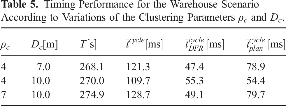
Timing Performance for the Warehouse Scenario According to Variations of the Clustering Parameters ρ _c and D _c .

ρ c	D c [m]	$\overline{T}\left[\mathrm{s}\right]$	${\overline{t}}^{cycle}\left[\text{ms}\right]$	${\overline{t}}_{DFR}^{cycle}\hspace{0.17em}\left[\text{ms}\right]$	${\overline{t}}_{plan}^{cycle}\hspace{0.17em}\left[\text{ms}\right]$
4	7.0	268.1	121.3	47.4	78.9
4	10.0	270.0	109.7	55.3	54.4
7	10.0	274.9	128.7	49.1	79.7

A representative example of the reconstructed map results shown in Figure 10 and the explored map volume over time is shown in Figure 6(d). A minimum coverage ratio of ${\vartheta }_{\mathcal{M}}=99.98\%$ was achieved for all test configurations. The APN size growth is depicted in Figure 6(h), which contained an average of 346 nodes and 21,494 edges, with an edge density factor of 0.374.

Figure 10.

The reconstructed map of the Warehouse scenario colorized by voxel height. The maximum height of displayed voxels is truncated for visual clarity.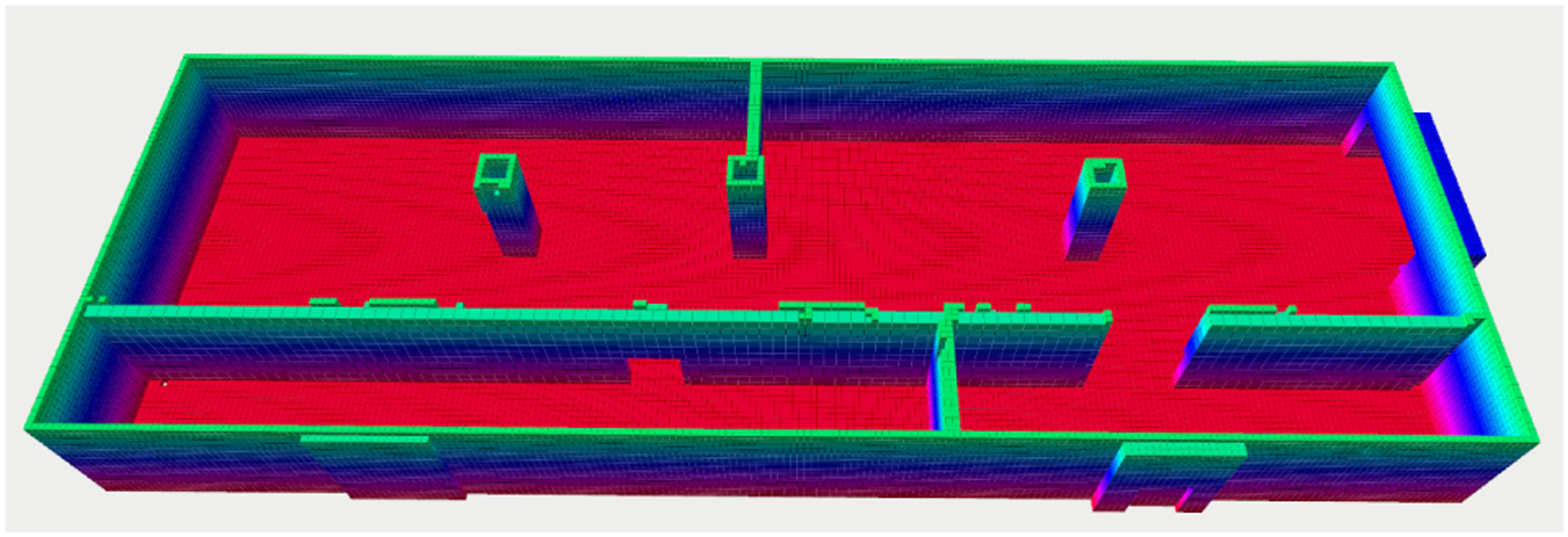

The computation time per cycle is plotted in Figure 7(d) and summarized in Table 4. Similar to the Ind. Plant scenario, the time spent on APN regulation remains within a bounded range despite the increasing size of the map and APN. The exploration time performance results are summarized in Table 4, requiring an average exploration time of $\overline{T}=268.1\mathrm{s}$ and average planning cycle time ${\overline{t}}^{cycle}=121.3\text{ms}$ . A more detailed breakdown of the processing times per sub-procedure is shown in Figure 7(h).

Different clustering parameter variations were applied and the resulting time performance is summarized in Table 5. The average exploration time did not significantly change between parameter variations, indicating the low sensitivity of these parameters. The primary effect of the variations was on the per-cycle computation time, though the differences were relatively minor. Using the values ρ _c = 4 and D _c = 10.0, the cycle time was nearly evenly distributed between differential regulation, ${\overline{t}}_{DFR}^{cycle}$ , and planning, ${\overline{t}}_{plan}^{cycle}$ . The other parameter combinations increased the planning time, but only by a small amount.

4.5. Ablation studies

Ablation studies were devised to discover insights into the performance and behavior of our methodology. These primarily focus on the performance effects of pruning and hierarchical planning, and are divided into two test cases as follows:

• Case 1: pruning disabled;

• Case 2: pruning and hierarchical planning disabled.

For Case 1, the pruning stage described in Section 3.3.3 was disabled from the system while keeping all other operations intact. In Case 2, the use of hierarchical planning was also disabled, where planning instead operates on all candidate NBVs within the APN to find the non-myopic global exploration sequence without being informed by the topological cluster regions. Case 1 and Case 2 were evaluated using the Maze Scenario with map resolution 0.2 m, and Case 2 was further evaluated using the Warehouse Scenario with map resolution 0.4 m to observe the effects at large-scales. The baseline of each case corresponds to the previous parameters and results without ablations for each scenario, as described in the previous subsections. Each case was performed 5 times to compute the statistical averages.

The results are reported in Table 6 in terms of percentage increase over the respective baselines. To quantify the differences in NBV coverage efficiency, an additional measure ${\theta }_{\mathcal{F}}^{nbv}$ is defined to be the average ratio of NBVs to frontiers. Additional metrics are reported in terms of the percent difference for the total execution time $\overline{T}$ , and the individual processing times of ${\overline{t}}^{cycle}$ , and ${\overline{t}}_{plan}^{cycle}$ , along with the total distance traveled, d _T .

Table 6.

Summary of Ablation Case Performance in Terms of Percent Difference from Baseline. $\overline{T}$ and d _T are the Completion Time and Distance, Respectively. ${\overline{t}}_{DFR}^{cycle}$ and ${\overline{t}}_{plan}^{cycle}$ Are the Processing Time Spent for DFR and Planning, and ${\theta }_{\mathcal{F}}^{nbv}$ Is the Average Ratio of NBVs to Frontiers.

	$\overline{T}$	${\overline{t}}_{DFR}^{cycle}$	${\overline{t}}_{plan}^{cycle}$	${\theta }_{\mathcal{F}}^{nbv}$	d T (%)
Maze:
Case 1	3.0%	0.3%	65.0%	96.7%	28.3
Case 2	−0.3%	1.0%	86.9%	104.2%	−2.4
Warehouse:
Case 2	33.9%	1.2%	481.5%	65.4%	37.7

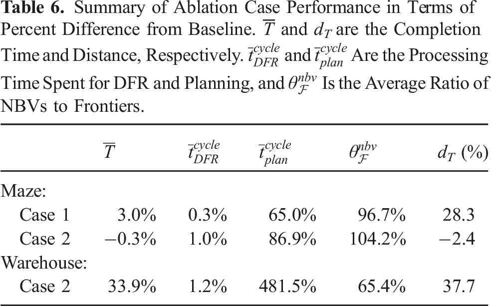
For the Maze Scenario, removing the pruning stage (i.e., Case 1) prevented the analysis and removal of redundant NBVs that covered no exclusive information, increasing the average NBV to frontier ratio ${\theta }_{\mathcal{F}}^{nbv}$ by 96.7%. The APN contained an average of 11.8 redundant NBVs with a maximum of 33, compared to 0 for the baseline. The preservation of these views then introduced larger problem sizes for planning, which is demonstrated by the increased time ${\overline{t}}_{plan}^{cycle}$ shown in Table 6. Furthermore, the inclusion of redundant views also decreased the efficiency of each planning cycle, since wasteful motions can occur when navigating towards views with redundant coverage. These effects can be observed by the total exploration distance d _T , which increased by 28.3% for this test. The DFR processing time ${\overline{t}}_{DFR}^{cycle}$ did not significantly change for this or the other test cases, owing to the low computational cost of the pruning approach. Slight increases can be seen though, as the increased nodes led to more edge computations.

Using Case 2 for the Maze Scenario, the results show a significant increase in average planning time per cycle by 86.9%, while the total completion time did not significantly change. This can be explained intuitively, as the use of hierarchical planning serves as an approximation of the underlying view sequence, decreasing the problem size but also introducing resolution losses. Planning over the full set of NBVs allowed finer optimization resolution, but at the cost of longer computations. Still, given the smaller scale of the Maze scenario, the increased computations were not large enough to greatly impact its overall performance.

For Case 2 applied to the Warehouse Scenario, as also summarized in Table 6, the increased planning complexity when pruning and hierarchical planning are disabled becomes very apparent. An increase of 481.5% to the planning time per cycle was experienced, with the maximum planning time taking over 4.5s compared to the maximum of 374 ms for the baseline case. For the baseline case, planning was performed over an average of 21.2 clusters, and 13.7 NBVs. Comparatively, Case 2 planned over an average of 57.1 NBVs while omitting the cluster planning stage.

Furthermore, the total completion time $\overline{T}$ increased by an average of 33.9% and the total distance traveled d _T increased by 37.7%. Both of these values indicate the decreased optimality of the planned paths. The average number of evolutionary generations for view planning increased by a factor of about two, where the maximum generation threshold N _stall was reached. The maximum generation threshold was set to 5000, but was never exceeded in any case. Note that in all runs, the sign of the percentage values never change, that is, Table 6 accurately show that, overall, the results of these ablation studies indicate the effectiveness of pruning and the hierarchical strategy in both reducing the overall computational costs and increasing the exploration efficiency and scalability.

4.6. Discussions

The experimental results show that our approach has the ability to iteratively update the APN and replan the exploration path at an average rate of at least 20 Hz for the two smaller scale scenarios (Apt. and Maze), and at least 5 Hz for the larger scales (Industrial Plant and Warehouse). However, the difference between these cycle rates is not primarily due to the larger environment sizes. Instead, the larger sensor view volume and higher maximum velocities are the more significant factors, which result in a larger amount of map data for processing per cycle, but these factors are not directly related to the environment size. This helps to explain the scalability of our approach for larger environments.

For the smaller environments, most of the planning time is spent on local view planning (see Figures 7(e) and 7(f)), This is due to the relatively few clusters needed to partition the nodes, resulting in trivial cluster planning instances. However, planning directly over all NBVs can quickly become intractable as the map size increases, either resulting in unacceptably large processing times, or would otherwise require premature search termination that degrades the planning quality.

The hierarchical planning strategy of APN-P helps to mitigate the complexity by keeping the problem size manageable. Furthermore, planning convergence is further accelerated by initializing each planning cycle from the partially optimized solution of the previous cycle. This reduces the need to introduce further problem simplifications or approximations that would decrease the planning quality. These effects are demonstrated by the results shown in Figures 7(d) and 7(h). The distributed planning time remains relatively low and does not exhibit continually increasing growth, despite the increasing size of the map and APN as shown in Figures 6(h) and 6(d).

The frontier-guided information gain and sampling strategy of DFR provides an effective way to avoid the prohibitively high computation costs for analyzing information gain by the existing (compared) approaches and to balance processing time per cycle and update rates. This enables maximized coverage of the unknown map regions to be maintained at high update rates, providing the necessary knowledge needed for non-myopic planning.

4.7. Further comparative study

We focus here on a comparative study between our APN-P system and the TARE system (Cao et al., 2021), as both use hierarchical planning. The TARE system uses a top-down approach to divide a map into even cuboid subspaces and conduct two-level planning: global planning to find a sequence to visit each subspace and local planning within each subspace. In contrast, our APN-P system uses a bottom–up approach which computes the reachable configurations first, then analyzes their structure on the fly to determine the topological structure.

To compare the performance between APN-P and TARE, each system was evaluated within the Corridors Scenario shown in Figure 11(a), which has the maximum dimensions of 130 × 100 × 4 (m³). The open-source software of TARE was used for its implementation which also includes a test application and configuration parameters tuned specifically for the Corridors Scenario. Though TARE is capable of being adapted for use with either ground or aerial vehicles, we note that the open-source software only supports ground-based exploration. For this reason, TARE was tested using an unmanned ground vehicle (UGV) equipped with a Velodyne Puck LiDAR scanner with a horizontal FoV of 360^◦ and vertical FoV of 30^◦, and the APN-P was tested using the Firefly MAV modified to use the Velodyne LiDAR instead of the stereo camera sensor from the previous scenarios. Each system used a map resolution of 0.5 m for occupied surface representation.

Figure 11.

The Corridors Scenario with the maximum dimensions of 130 × 100 × 4 (m³).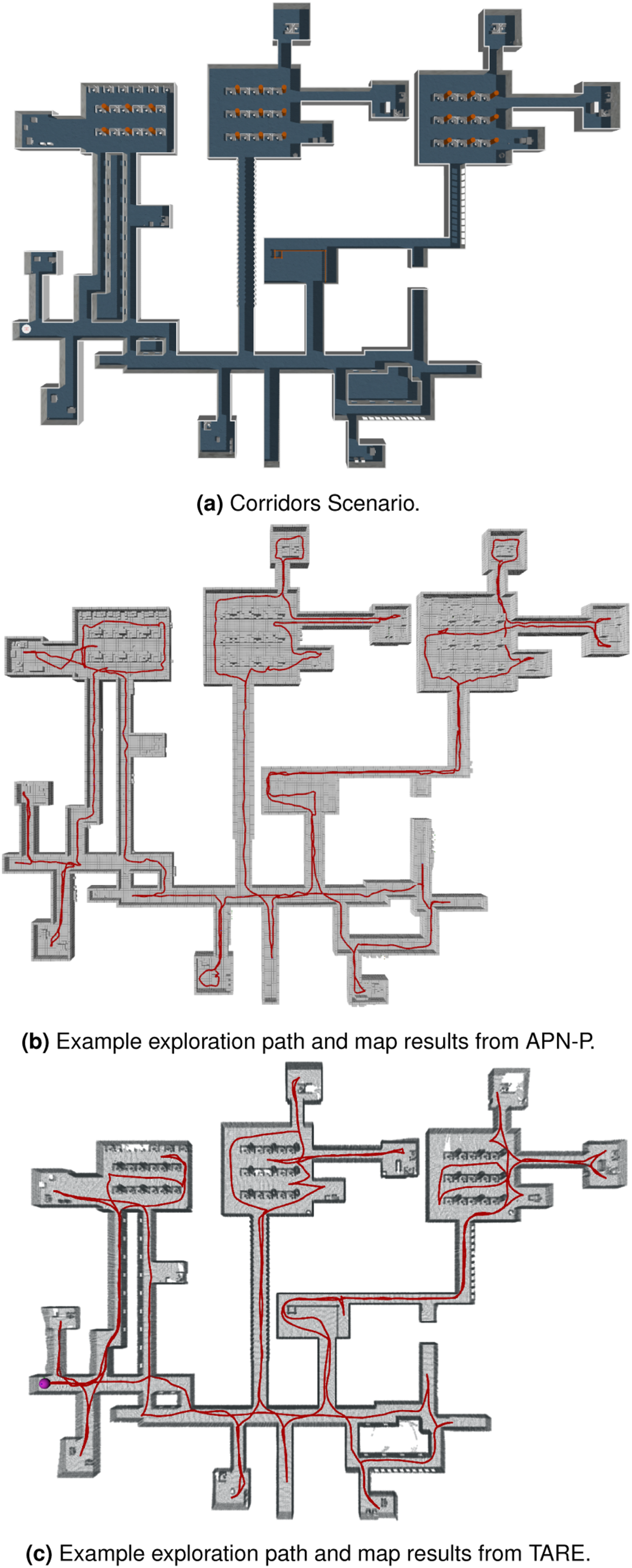

Given the different robots used to evaluate each system, additional steps were taken to ensure fair comparison between the approaches. To equalize the robot workspaces, modifications were made to our approach to restrict all robot configuration of the APN to fixed plane equal in altitude to the height of the sensor on the UGV. The altitude restriction was enforced by restricting the vertical dimension of all sampling and motion planning procedures according to the fixed altitude. This ensures all APN nodes and their edges will lie on the same traversal plane as the UGV sensor, along with any trajectories planned between APN nodes. Additionally, collision detection was updated to check for obstacles along the ground plane, such that configurations are treated as a collision if the space directly underneath is not traversable. This ensures any valid configuration will be valid for both vehicles, and that the MAV does not traverse any path that could not be traversed by the UGV. Further, each vehicle was limited by a common maximum velocity of 2 m/s.

The average results over five tests for each method are summarized in Table 7 comprised of the total exploration time $\overline{T}$ (s), cycle processing time ${\overline{t}}^{cycle}$ (ms), and distance traveled d _T (m). The mapping results are also reported in terms of the final map volume (m³) and exploration efficiency ${\eta }_{\mathcal{M}}$ (m³/s). We note that given the different map representations between approaches, the map volume term refers only to the occupied map space from covered surfaces.

Table 7.

Key Performance Metric Result Comparison Between APN-P and TARE Using the Corridors Scenario.

	APN-P	TARE	Diff (%)
$\overline{T}\left[\mathrm{s}\right]$	597.5 ± 39.2	746.6 ± 39.2	−20.0
${\overline{t}}^{cycle}\left[\text{ms}\right]$	96.7 ± 7.7	315.6 ± 7.2	−69.4
d T [m]	941.2 ± 57.2	1174.5 ± 86.5	−19.9
Map vol. [m3]	6472.9 ± 16.1	5283.4 ± 7.5	22.5
${\eta }_{\mathcal{M}}\left[{\mathrm{m}}^3/\mathrm{s}\right]$	10.8 ± 0.4	8.1 ± 0.5	33.7

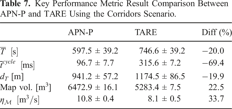
Both systems were able to consistently explore the full environment, with example exploration paths and map coverage results for each system shown in Figures 11b and 11(c). TARE took an average total time of 746.6s for exploration and APN-P took an average of 597.5s, an improvement of around 20%. Though both methods were able to explore all traversable regions, APNP-P also achieved higher environment coverage with a 22.5% increase in the explored map volume, which can be seen from comparing the mapping results in Figure 11. Additionally, the average cycle processing time for TARE was 315.6 ms, while APN-P was more than three times as fast at 96.7 ms. From these comparisons, APN-P demonstrates faster exploration with higher coverage completeness while still using less processing time per cycle.

Further results of APN-P are shown in Figure 12 regarding the map exploration progress over time compared to TARE (Figure 12(a)), with cycle processing times plotted in Figure 12(b) and statistical breakdown of subprocess times shown in Figure 12(c). Figure 12(a) shows the APN-P explores the map at a faster rate throughout execution, where TARE has longer periods of low gain (indicated by flat peaks in the plot). This effect is most prominent for TARE toward the end of the run in Figure 12(a), where significant backtracking is needed to reach distant regions where coverage was not completed before moving to other regions.

Figure 12.

Representative performance results for the Corridors Scenario from APN-P.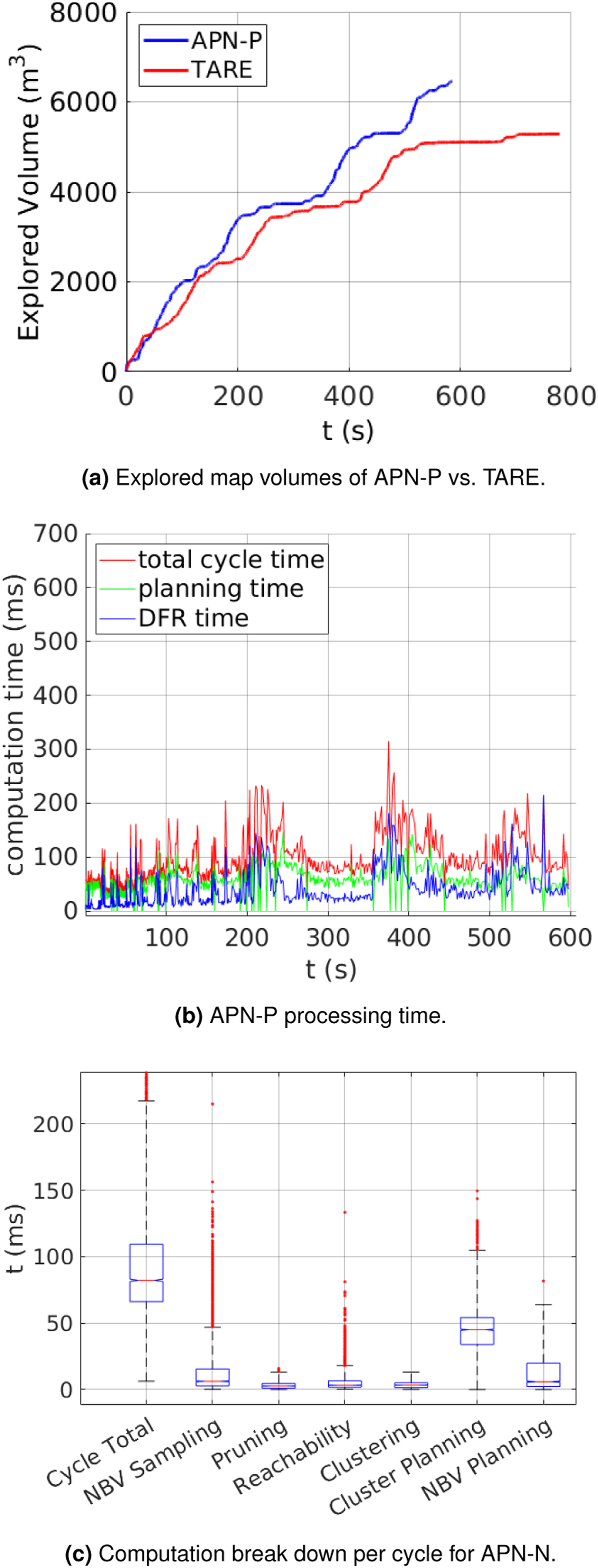

The average time APN-P spent on DFR was 32.7 ms, and planning took an average of 10.85 ms for global cluster planning, and 38.35 ms for local NBV planning. For each planning instance, the global plan was optimized over an average of about 7.4 clusters, with the local plan optimized over an average of five NBVs. In comparison, TARE used an average of 283.5 ms spent to update its environment representation, over eight times longer than APN-P, and used an average of 27.1 ms for global planning and 5.1 ms for local planning. While the planning times for TARE are slightly shorter than the APN-P’s, they do not appear to be as high quality as those planned by the APN-P, as indicated by the faster exploration times in Table 7. This may be explained by the way TARE uses simplified subspace representations with regular size and spacing and do not consider the underlying reachability given their top–down approach. This approach can reduce the computation times, but can cause lower quality paths to be planned such as when adjacent clusters or views are not directly reachable from each other, as the method initially assumes.

5. Conclusions and future work

This paper has presented the Active Perception Network (APN), serving as a topological roadmap of the dynamically changing exploration state space, the differential regulation (DFR) update procedure that incrementally adapts the APN to the changing environment knowledge, and an exploration planner APN-P, which leverages the APN to find non-myopic exploration sequences through the APN.

The results demonstrate the efficiency of DFR in performing each cyclic update and its scalability with increasing map sizes. In comparison to several state-of-the-art approaches, the APN-P consistently demonstrated improved performance in terms of total exploration time and coverage completeness. The improved performance was achieved over a variety of different environments, both indoor and outdoor, with only minor parameter adjustments between them. We expect to make all implementations of the presented work available as open-source, including the full development framework it was built upon (briefly introduced in the Appendix).

Several areas of future work have been identified. The testing and analysis of this work assumed ideal localization without noise or uncertainty to facilitate analysis of the theoretical performance separately. In practice, noise and uncertainty cannot be ignored. However, our methodology is well-suited to be extended for handling noise and uncertainty in terms of the approach and through the extensibility of our software framework.

Handling uncertainties and noise would involve the incorporation of Active SLAM strategies, which often make use of graph structures. The APN and DFR models can be adapted, for example, to consider additional features like localization landmarks for visibility analysis, and additional cost and reward functions can be associated to nodes or edges of the APN related to uncertainty analysis. DFR can then be modified to include additional stages to update the additional information aspects, while keeping the existing stages intact for computing the reachability space. The evolutionary planning approach can then be readily extended to perform multi-objective optimization that considers minimization of localization uncertainty. The high computational efficiency currently achieved provides much latitude for handling the increased computational costs. Further ablation studies and analysis of parameter sensitivity will help understand how to best tune their values to guide future developments that are generalizable to a wider range of environment scenarios and that reduce or eliminate the need for more parameter tuning.

Supplemental Material