Sage Journals: Discover world-class research

Abstract

Simultaneous Localization and Mapping (SLAM) refers to the common requirement for autonomous platforms to estimate their pose and map their surroundings. There are many robust and real-time methods available for solving the SLAM problem. Most are divided into a front-end, which performs incremental pose estimation, and a back-end, which smooths and corrects the results. A low-drift front-end odometry solution is needed for robust and accurate back-end performance. Front-end methods employ various techniques, such as point cloud-to-point cloud (PC2PC) registration, key feature extraction and matching, and deep learning-based approaches. The front-end algorithms have become increasingly complex in the search for low-drift solutions and many now have large configuration parameter sets. It is desirable that the front-end algorithm should be inherently robust so that it does not need to be tuned by several, perhaps many, configuration parameters to achieve low drift in various environments. To address this issue, we propose Simple Mapping and Localization Estimation (SiMpLE), a front-end LiDAR-only odometry method that requires five low-sensitivity configurable parameters. SiMpLE is a scan-to-map point cloud registration algorithm that is straightforward to understand, configure, and implement. We evaluate SiMpLE using the KITTI, MulRan, UrbanNav, and a dataset created at the University of Queensland. SiMpLE performs among the top-ranked algorithms in the KITTI dataset and outperformed all prominent open-source approaches in the MulRan dataset whilst having the smallest configuration set. The UQ dataset also demonstrated accurate odometry with low-density point clouds using Velodyne VLP-16 and Livox Horizon LiDARs. SiMpLE is a front-end odometry solution that can be integrated with other sensing modalities and pose graph-based back-end methods for increased accuracy and long-term mapping. The lightweight and portable code for SiMpLE is available at: https://github.com/vb44/SiMpLE.

Keywords

Light detection and ranging odometry simultaneous localization and mapping minimal configuration

1. Introduction

Simultaneous Localization and Mapping (SLAM) is the problem of localizing a mobile platform while constructing a map of its environment. Early work on the problem in robotics goes back to Leonard and Durrant-Whyte (1991). Durrant-Whyte and Bailey (2006) identified solving the SLAM problem as an essential step towards fully autonomous robots to estimate their position and orientation, or pose, within an environment. SLAM is a difficult problem as localization requires a map of the environment, and a pose estimate is required to construct the map. Pomerleau et al. (2015) recognized the accelerated interest in this problem since the introduction of laser scanners in the early 1990s. SLAM has become a prominent and expanding research field with applications in autonomous platform positioning (Cao et al., 2021; Lategahn et al., 2011), search and rescue robots (Chen et al., 2017a; Kleiner et al., 2006; Wang et al., 2018), indoor and outdoor mapping (Filipenko and Afanasyev 2018; Zheyuan and Uchimura., 2009), and has future applications in interplanetary exploration (Chen et al., 2017b).

SLAM is commonly divided into sub-problems, both of which have received significant attention. The first is a front-end, responsible for providing real-time odometry from incoming sensor information. This is also commonly referred to as recursive pose estimation as the registration result at time k is dependent on the result at time k − 1 and is therefore prone to accumulate drift over extended periods due to sensor measurement error and numerical errors introduced in pose estimation calculations. A real-time or post-processing back-end is usually employed to reduce the accumulated drift and correct the pose estimates. This is generally modelled as a batch or incremental optimization problem. The performance of the back-end solution depends on the accuracy of the front-end algorithm as large drift may cause errors in loop closure identification methods. The goal is to achieve accurate and real-time localization of the mobile platform within an unknown or known environment. For this paper, we focus on providing a front-end Light Detection and Ranging (LiDAR) odometry method that does not require significant configuration or tuning to achieve low-drift performance.

The localization and mapping problem continues to attract the interest of researchers as new sensors and methods are developed in the pursuit of more precise and robust solutions. The authors of this paper observe an increasing complexity of algorithms with larger configuration parameter sets. Increasing the size of the configuration parameter set tailors to the use case they are developed for. We eschew this and seek general applicability without tailored configuration.

This paper presents an efficient and accurate LiDAR odometry algorithm that provides a minimal configuration front-end only LiDAR odometry method. This algorithm performs among and better than most top-ranked LiDAR odometry methods benchmarked on the publicly available KITTI dataset by Geiger et al. (2012) and outperforms all methods in the MulRan dataset by Kim et al. (2020) and the UrbanNav dataset by Hsu et al. (2021). The solution is simple to understand, simple to implement, and simple to configure. Hence, we name the algorithm Simple Mapping and Localization Estimation or SiMpLE. Figure 1 illustrates the performance of leading LiDAR odometry methods, evaluated through benchmarking on the KITTI and MulRan datasets. The figure also displays the associated number of reported configuration parameters for each method. SiMpLE demonstrates superior performance compared to numerous open-source methods, all while boasting the smallest configuration set. This solution serves as a solid basis for seamless integration with other sensing modalities, such as IMUs or cameras, and can be effectively combined with a back-end to create a full SLAM solution.

Figure 1.

The state-of-the-art LiDAR odometry methods have similar performance but with a significant difference in the number of configuration parameters. Our solution, SiMpLE, has only five configurable parameters and performs among the top-ranked algorithms. The translational error for the KITTI sequences 00-10 (left) is as published by the respective methods. The translational error for the MulRan sequences (right) is as reported by Vizzo et al. (2023).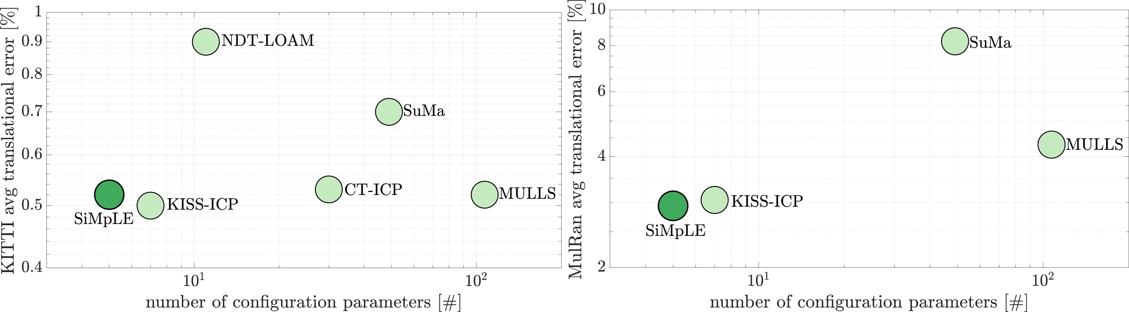

Unlike many published methods, we do not modify or tweak existing solutions or require complex pre-processing steps such as outlier removal or noise rejection. The formulation for SiMpLE is designed to use raw point cloud data. This continues previous work by using reward-based metrics to solve pose estimation problems as introduced in Phillips et al. (2021); Bhandari et al. (2023). The paper’s contributions are first to introduce a straightforward, and possibly the simplest, LiDAR odometry solution, showcasing state-of-the-art performance across different scenarios. Second, the paper offers an open-source, lightweight, portable, and readily accessible code implementing the method, available at https://github.com/vb44/SiMpLE.

This paper is organized as follows. Section 2 discusses the challenges of providing an accurate and real-time LiDAR odometry solution. Section 3 provides an overview of classical and modern SLAM algorithms. Section 4 formulates the SiMpLE algorithm. Section 5 benchmarks the performance of SiMpLE across publicly available datasets and a dataset recorded at the University of Queensland. Future work is detailed in Section 6 and concluding remarks are made in Section 7.

2. The challenges of providing accurate and real-time LiDAR odometry

SLAM methods employ a variety of sensing modalities to construct an understanding of the surrounding environment. LiDARs are commonly used as the prominent sensing modality due to their high accuracy, fast data acquisition rates, and increasing availability. Pomerleau et al. (2015) identified PC2PC registration, or scan matching, as the foundation of many front-end odometry algorithms. PC2PC registration aims to find the 6-DOF homogeneous transform consisting of the (roll-pitch-yaw) rotations and (x-y-z) translations that best align consecutive static point clouds in a timely manner. In an otherwise static environment, the relative transformation between the point clouds corresponds to the movement of the sensor and, consequently, the platform to which the sensor is rigidly mounted, for example, a car. When applied to successive point clouds obtained from a moving platform, this method enables the localization of the platform and the construction of a map of the environment using the relative transformation between each point cloud.

LiDARs provide a point cloud that represents the surrounding environment with a set of 3D Cartesian points and corresponding intensity values. New technologies such as Aeva’s FMCW LiDAR also provide per-point relative radial velocity (Aeva, 2022). However, these measurements contain no interpretable semantic information or association with the environment they represent. The ability to draw reliable and timely references from the raw data is limited, and the understanding of the point cloud is open to interpretation. Algorithms must be robust, safe, and reliable as they affect the quality of subsequent planning and control stages. There are several challenges associated with point cloud interpretation that inhibit the ability to provide accurate and real-time recursive pose estimates.

The accuracy of the result(s) interpreted from point cloud data is subject to various sources of uncertainty. The sensor itself will have a documented range measurement uncertainty. Per-beam intrinsic calibration parameters are only known to a level of certainty and must be correct for high-quality point clouds as considered by Sheehan et al. (2012) and Bergelt et al. (2017). The sensor’s installation involves assumptions about its position, leading to uncertainty in its extrinsic registration to the platform. Phillips et al. (2015) and D’Adamo et al. (2018) emphasize the importance of accurate registration for providing a correct interpretation of the point cloud. These uncertainties combine and propagate to provide an erroneous representation of the environment.

The environment itself may provide various challenges. It is difficult to detect motion in a featureless environment using LiDAR points only. PC2PC registration algorithms require unique features in the environment to estimate the transformation between successive point clouds. This is a well-known problem of LiDAR odometry, often referred to as the corridor mapping problem explored by many researchers including Diosi et al. (2005), Zang et al. (2006), and Yu and Zhang (2018).

Moreover, algorithms relying on feature matching often assume a static environment. Static environments are well captured by point cloud data as the range measurements provide a true representation of the environment. While point cloud data can accurately represent static environments due to the precise range measurements, many real-world settings encompass dynamic elements. These dynamic elements introduce complexity in understanding moving objects within the scene, making the interpretation of the environment a challenging task. When assuming a static environment with dynamic objects, incorrect feature matching occurs, leading to inherent errors in the pose estimates. This highlights the importance of accounting for dynamic elements in the environment to achieve more accurate and reliable odometry results.

Reliable estimates should be provided under adverse environmental conditions. The quality of the point cloud measurements is dependent on weather conditions. Heinzler et al. (2019) and Kutila et al. (2016) report degraded sensor performance in the presence of rain and fog. Phillips et al. (2017) detail similar findings in the presence of dust. LiDAR sensors commonly struggle to distinguish spurious data points, resulting in a misrepresentation of the environment that necessitates additional processing. These errors can compromise derived point cloud geometric properties, including surface normals.

A LiDAR odometry method should be agnostic to the sensor used to generate the point clouds. Many 3D LiDAR products are commercially available and provide unique scan patterns, point cloud density, fields of view, and resolution. The scan pattern demands further consideration since point cloud measurements become sparser at longer ranges and significantly denser close to the sensor. This often affects the ability to extract features for matching scans. Mechanical rotating LiDARs have a scan pattern that does not move linearly with the platform. The ring pattern from rotating LiDARs causes incorrect correspondence between scans, leading to pose estimation errors.

A requirement for autonomous systems is to interpret sensor data in real-time at rates faster than the planning and control decisions. More time occupied by the perception stage decreases the available time for making critical decisions or introduces lag where decisions are made from outdated beliefs. The accuracy is often decreased to increase processing times, introducing the risk of making non-optimal decisions in subsequent stages. This is made challenging with modern 3D LiDARs providing millions of points per second at frame rates between 10 and 20 Hz. The hardware on many platforms is limited, reducing the computational resources available for interpreting the data.

In common applications of PC2PC registration, addressing a combination of these challenges is necessary to achieve robust, accurate, and reliable pose estimates. Nonetheless, we argue that simpler solutions are feasible and will prove more effective, efficient, and robust.

3. An overview of localization algorithms

The following provides a review of LiDAR odometry algorithms and approaches to overcoming the challenges previously identified. Attention is drawn to the increasing complexity of algorithms, and potential gaps are identified and addressed in the SiMpLE formulation in the next section.

3.1. Classical approaches

The Iterative Closest Point (ICP) algorithm, introduced by Besl and McKay (1992), is the most common method for solving the PC2PC registration problem. The algorithm iteratively searches for the homogeneous transformation that minimizes the distance error between the source and target point cloud. The method assumes data association and a static environment. ICP is simple to implement and provides accurate results using noise-free point clouds in static environments. However, these conditions are not typically observed in real-world operating environments. In its raw form, the algorithm also possesses flaws; it requires a good initial transformation guess, incurs high computational costs, and is susceptible to local extrema. Other limitations stem from its utilization of an error-based metric and dependence on assigning correspondences between point clouds, see Phillips et al. (2021).

Researchers have introduced numerous variants of ICP to overcome these limitations, see Rusinkiewicz and Levoy (2001). KISS-ICP by Vizzo et al. (2023) uses an adaptive threshold for data association and outlier rejection for highly accurate alignment of the point clouds. Donoso et al. (2017) compared 20,736 distinct ICP variants resulting from permutations and combinations of pipeline steps applied to three different scenes (data sets). The findings indicate, among other things, that no single variant stands out as the best, highlighting that performance is closely linked to both the data and the algorithms used. The validity of using ICP for PC2PC registration is brought into question by these findings. Nevertheless, it persists and continues to be utilized in new approaches, as seen in Clotet and Palacín (2023).

The introduction of the Normal Distributions Transform (NDT) by Biber and Straßer (2003) overcomes some shortcomings of the ICP algorithm. NDT does not assume correspondence between scans and uses a probabilistic reward-based framework instead of the error-based metric in ICP. The point cloud is divided into voxels of a grid size selected by the user, and the mean and covariance of each grid are calculated and used to assign a reward value when matching a consecutive scan. Using reward instead of error and making no assumption about the correspondence allows for robustness in dynamic environments. However, Magnusson et al. (2007) note the optimal size and distribution of cells depend on the shape of the input data and on the application. NDT is fast, but Ulaş and Temeltaş (2013) identify discontinuities in the surface representation due to discretization.

To reduce the effect of discretization, Biber and Straßer mention the use of multiple grids at the cost of compromising the algorithm’s speed. The grid size selection is also a sensitive parameter, as discussed by Kaminade et al. (2008). Hong and Lee (2017) reduce the effect of the grid size parameter by introducing a probabilistic Normal Distributions Transform representation that uses the probabilities of point samples instead of only building distributions for the divided grids, allowing for all points to contribute towards the reward evaluation. Even though the minimum point requirement to form distributions is removed, the presence of the cell size remains. Other attempts such as by Ulaş and Temeltaş (2013) use multi-resolution grid sizes to overcome this issue.

3.2. Modern approaches

PC2PC methods, like ICP and NDT, rely solely on the raw point cloud data. However, many modern techniques extract additional geometric properties from the point cloud to complement and enhance the accuracy and convergence time of ICP or NDT scan matching. Nonetheless, this often introduces more parameters and increased complexity. Feature-based methods, for example, extract lines, planes, and landmarks from the point cloud to improve scan matching. They are commonly used as a coarse registration method, providing a good initial estimate for fine registration methods like NDT and ICP (Cheng et al., 2018; Huang et al., 2021). LOAM, introduced by Zhang and Singh (2014), is a popular method utilizing feature extraction. It extracts edge and planar points to achieve accurate scan alignment, ranking among the top LiDAR odometry methods. Similarly, F-LOAM developed by Wang et al. (2021), constructs a local edge and plane map to facilitate feature-based registration.

Many methods provide a full SLAM solution. MULLS is a state-of-the-art method proposed by Pan et al. (2021). At its core, the method uses a feature extraction-based front-end with a multi-metric linear least square ICP algorithm. Feature extraction involves classifying various feature points such as the ground, façade, pillars, and beams. The back-end uses hierarchical pose graph optimization composed of sub-maps registered using TEASER++ by Yang et al. (2020) for constructing global maps. The complete algorithm is composed of many stages with 107 identified configurable parameters. While the performance is promising and provides real-time results, the algorithm is complex and requires appropriate parameter selection for ideal performance depending on the environment.

Similar approaches are taken by other methods such as Efficient LiDAR odometry by Zheng and Zhu (2021). It is a front-end method only, using a multi-stage pipeline consisting of spherical projection, ground segmentation, range-adaptive normal estimation, bird-eye-view projection, and ICP at its core for point cloud registration. As before, many configurable parameters are involved for each stage.

Alternative representations are often used to overcome the challenge of constructing large maps. A common approach is to use surfel-based maps and is implemented by robust approaches such as SuMa by Behley and Stachniss (2018) and Wildcat by Ramezani et al. (2022).

In an effort to reduce the configuration effort of handcrafted algorithms, Yin et al. (2020) use a deep learning foundation for feature extraction and keyframe selection to aid in point cloud matching. Deep learning methods also extend geometric feature extraction to recently published semantic-based approaches such as SuMa++ by Chen et al. (2019), and PSF-LO by Chen et al. (2021), allowing for dynamic object detection and accurate mapping in featureless environments. However, the complexity is increased with the design of the deep learning model architecture and providing sufficient training data for high-accuracy performance. Examining errors also becomes difficult as the output needs to be back-traced through many layers, which is not always possible using deep learning methods. Considerable research has been conducted into deep learning frameworks by Wang et al. (2017), Li et al. (2019), Li and Wang (2020), and Zheng et al. (2020).

3.3. The increasing complexity of SLAM methods

There is a noticeable trend in SLAM research towards increasingly complex algorithms that achieve similar performance to existing methods. However, very few approaches offer manageable and meaningful parameter sets along with straightforward and implementable methodologies, particularly when it comes to examining LiDAR odometry algorithms. Even widely used solutions such as Google Cartographer acknowledge the challenges of parameter tuning, stating ‘Tuning Cartographer is unfortunately very difficult. The system has many parameters many of which affect each other’ (Cartographer, 2022). Such complexity is far from ideal, often leading to post-processing and iterative tuning to achieve an optimal solution or tailoring algorithms to work with specific use cases. Our approach aligns with the philosophy of KISS-ICP (Vizzo et al., 2023), which advocates for a return to fundamental techniques to decrease complexity. This strategy enables easier identification of failure modes and ensures the algorithm remains user-friendly across a wide range of sensor types and environments.

4. The SiMpLE algorithm

SiMpLE is a scan-to-map registration algorithm inspired by our previous work in applying reward-based metrics for pose estimation problems using point cloud data in Phillips et al. (2021) and Bhandari et al. (2023). The algorithm rewards trajectories that locate new point cloud measurements in proximity to previously mapped point cloud measurements. We use scan-to-map instead of scan-to-scan registration to maximize the overlap between previous and new point clouds as the spatial resolution of LiDARs is known to reduce with distance, decreasing the overlap between consecutive scans (Mendes et al., 2016). The map keeps a temporal history of previous scans that is used to register against new point clouds, as detailed further below. The following three subsections detail the three steps of the SiMpLE algorithm.

4.1. Step 1: Input scan spatial subsampling

The first step is to spatially subsample the new scan, P _k, with a radius, r_new, to establish P′ _k. This step can be skipped given adequate computational resources, or the absence of a requirement for real-time computation (e.g. offline odometry or map generation). The spatial subsampling method is chosen in favour of traditional random sampling or voxel-based approaches (PCL, 2020) which can introduce aliasing in discretising the scene. This approach has been shown to considerably reduce the size of the point cloud while marginally reducing the information content of the environment, needed for accurate scan registration. The provided implementation uses a KD-tree (Blanco and Rai, 2014) to achieve fast removal of points. The pseudocode is displayed in the appendix in Algorithm 2. A minimum range filter can be optionally used here to remove sensor ranges close to the sensor, specified by the r_min parameter. This allows for a significant reduction in point cloud size and consequently helps improve computational performance. This parameter is further explored in Section 5.6.

4.2. Step 2: Point cloud-to-map registration

The second step is to register the subsampled new scan, P′ _k, to the existing subsampled map, M′ _k−1. This is obtained by estimating the frame transform, $T_{1 \to k}^{⋆}$ , that best locates the new scan within the existing map.

The scan-to-map registration step comprises two components: (i) an objective function used to score a pose estimate hypothesis and (ii) a search algorithm used to explore the pose hypothesis space for the highest-scoring pose estimate.

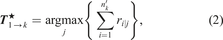
The SiMpLE objective function is predicated on the belief that the most likely pose estimate, $T_{1 \to k}^{⋆}$ , is that which locates new subsampled scan points, P′ _k, within the closest proximity to existing subsampled map points, M′ _k−1. This is a reward-based objective function that the algorithm seeks to maximize. This is a fundamentally different approach to an error-based objective function that would penalize pose estimates that locate points further from existing map data as thoroughly discussed by Phillips et al. (2021). The ICP formulation holds in static environments where there is expected to be a direct correspondence between point cloud measurements in the new scan and the existing map. However, this direct correspondence does not hold in most real-world scenarios, such as in the presence of noisy measurements, occlusion, partial overlap, and dynamic objects. Overcoming these real-world challenges introduces variants of ICP that propose various additional steps to handle such situations. The proposed change to a reward-based metric means that measurements that are not consistent between the new scan and the existing map do not detract from the true pose solution as they provide no reward.

Figure 2 depicts the objective function as it is applied to the j-th pose estimate, ${\hat{T}}_{1 \to k, j}$ . This estimate locates the i-th point of the new subsampled scan, which is denoted as p′ _k, _i|j. The closest existing map point to p′ _k,i|j is denoted as m′ _k−1, _i|j, with the Euclidean distance between these two points being,

d_{i | j} = ‖ p_{k, i | j}^{'} - m_{k - 1, i | j}^{'} ‖ .

(1)

Figure 2.

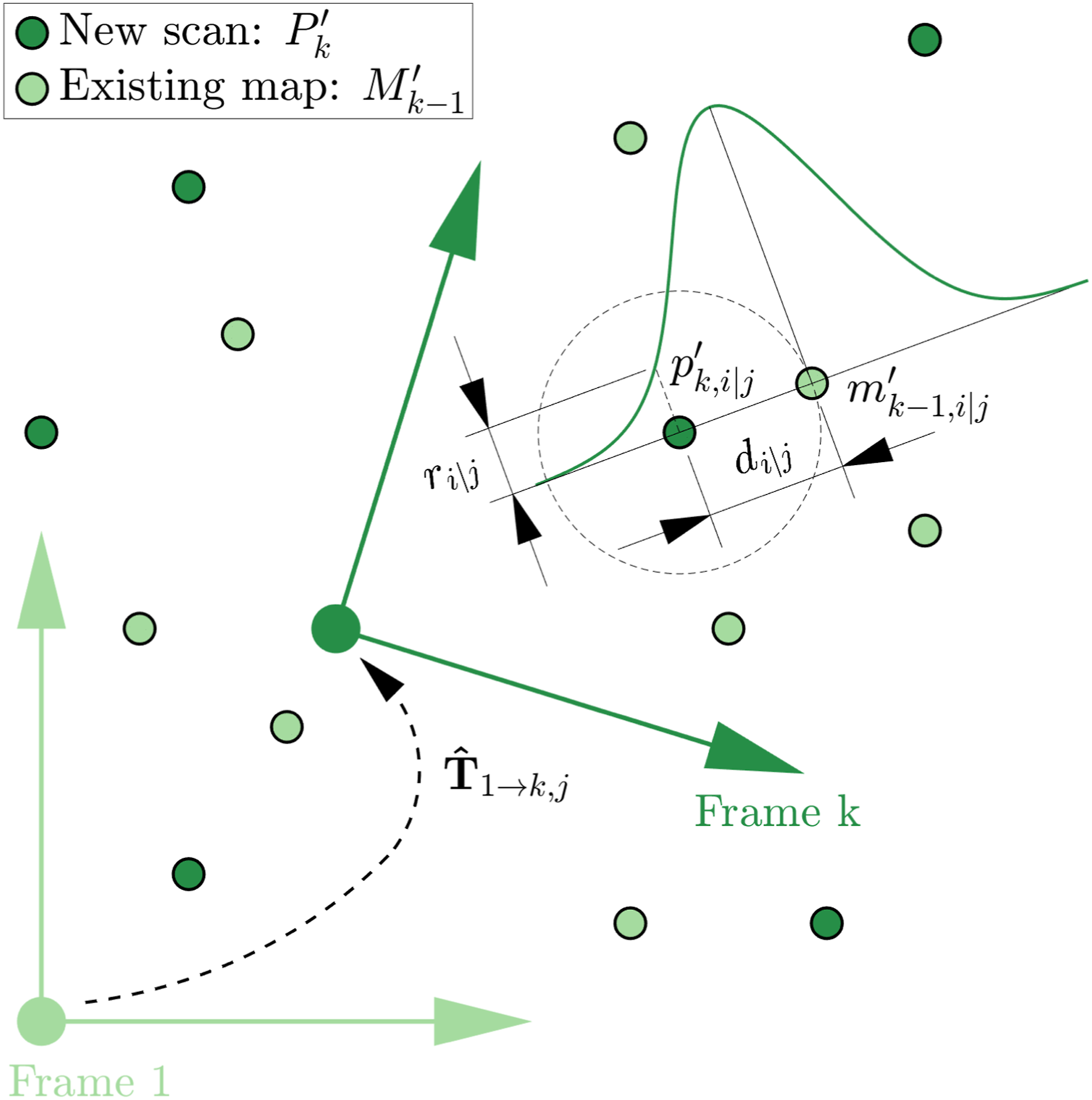
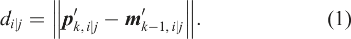
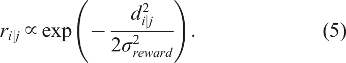
The subsampled new scan, P′ _k, is shown as located with the j-th pose estimate, ${\hat{T}}_{1 \to k, j}$ . The i-th point, p′ _k, _i|j, is rewarded with r_i|j, as determined as a function of proximity, d_i|j, to its nearest neighbour, m′ _k−1, _i|j, in the existing map, M′ _k−1. The overall reward of the pose hypothesis is determined by summing the reward, r_i|j, for all $n_{k}^{'}$ points in P′ _k.

A reward Gaussian is overlaid which illustrates the reward, r_i|j, decreasing as the distance between points, d_i|j, increases. The SiMpLE objective function seeks to find the transformation that maximizes the sum of r_i|j over all $n_{k}^{'}$ points of the subsampled new scan,

T_{1 \to k}^{⋆} = \underset{j}{argmax} {\sum_{i = 1}^{n_{k}^{'}} r_{i | j}},

(2)

where

\begin{array}{l} r_{i | j} = N (d_{i | j} | 0, σ_{r e w a r d}) \end{array}

(3)

\begin{array}{l} = \frac{1}{\sqrt{2 π σ_{r e w a r d}^{2}}} \exp (- \frac{d_{i | j}^{2}}{2 σ_{r e w a r d}^{2}}) . \end{array}

(4)

Furthermore, the normalizing constant can be discarded without affecting the result,

r_{i | j} \propto \exp (- \frac{d_{i | j}^{2}}{2 σ_{r e w a r d}^{2}}) .

(5)

The method described in this step is summarized in the appendix in Algorithm 3 and is closely related to the formulation of ICP, whereby the closest point is used. However, instead of directly minimizing the error between the point cloud measurements, here, points are rewarded for being close to other points. This single difference eliminates the need for point cloud pre-processing steps such as random sample consensus used for ground plane fitting by Pan et al. (2021), classification, clustering, segmentation, and all associated configurable parameters.

A search algorithm is required to find the highest-scoring pose estimate. The SiMpLE objective function does not require a specific search algorithm, and various algorithms are suited to this task, including gradient, simplex, and particle filter-based methods. While gradient-based solvers are susceptible to finding local extrema, we have found they are suitable because the transformation between successive scans is small for high-frame rate LiDAR scanners.

The implementation presented in this paper uses the Broyden–Fletcher–Goldfarb–Shanno (BFGS) Quasi-Newton optimization solver to search for the 6-DOF pose that best aligns the point cloud to the local map. The BFGS Quasi-Newton implementation performs an unconstrained optimization of the objective function using approximate derivatives starting at a provided seed described further below. The search termination condition is a user-defined parameter, ɛ_tol, which is a threshold for the minimum change in the registration reward between successive estimates before stopping the search. Dlib’s open-source implementation of BFGS Quasi-Newton by King (2009) is integrated with the described objective function.

Pose search algorithms rely on having a good initial guess, or seed, to avoid finding local extrema. A constant velocity model is used in SiMpLE’s implementation to provide an initial guess for the pose search algorithm. Given the initial pose, T _1→1 = I_4×4, is at the origin of the map frame, the initial guess for T _1→k is given by,

{\hat{T}}_{1 \to k} = T_{1 \to (k - 1)} Δ,

(6)

where Δ is the relative transformation of the previous solution.

Δ = T_{1 \to (k - 2)}^{- 1} T_{1 \to (k - 1)} .

(7)

Alternative approaches include using an IMU to approximate the current pose given the previous estimate.

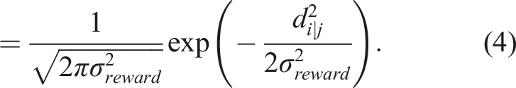
The parameter σ_reward influences the optimization solver’s solution. It effectively acts as a bandwidth parameter, similar to that used in a kernel density estimator, trading off between variance and bias in the surface of the reward function (Botev et al., 2010; Turlach, 1993). Section 5.5 demonstrates the insensitivity of σ_reward to small changes. The plots for two different values of σ_reward are displayed in Figure 3.

Figure 3.

The effect of changing the σ_reward configuration parameter. σ_reward is similar to the bandwidth parameter used in kernel density estimation in that it trades off between bias and variance. A small value for σ_reward (left) has the potential to under reward good hypotheses, whereas, a larger value of σ_reward can over reward weaker hypotheses. A sensitivity analysis is provided in Section 5.5 which shows that similar registration results are obtained over a wide range of σ_reward values.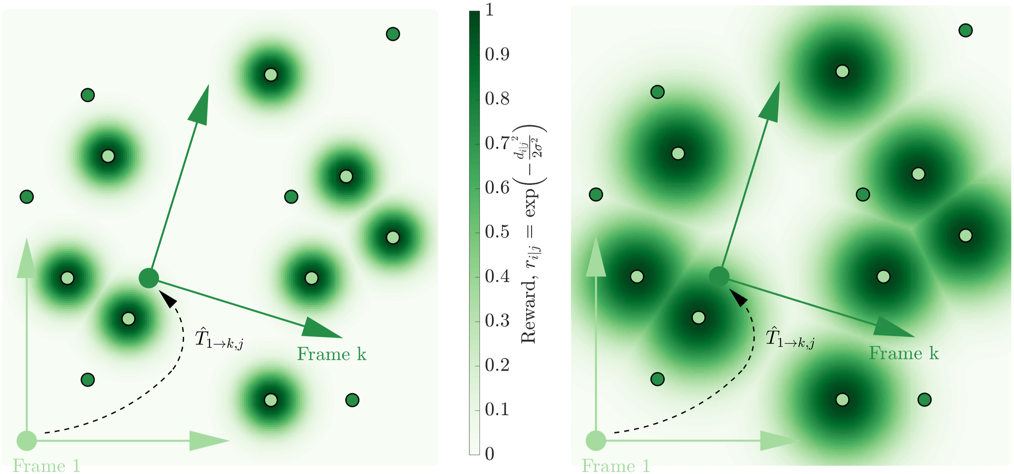

4.3. Step 3: Map update

Once the registration result has converged within ɛ_tol, the map is updated. The current subsampled scan, $P_{k}^{'}$ , is located within the map coordinate frame using the registration result, $T_{1 \to k}^{⋆}$ . The resulting points are added to the existing subsampled map, M′ _k−1, such that each point in the map maintains a spatial separation of r_map. Points outside the maximum range of the sensor, r_max, from the current pose estimate, are removed to maintain the size of the map. This parameter is dictated by hardware specification.

Scan-to-map registration is used to reduce the effects of the LiDAR’s scan pattern and maximize the overlap between the map and the new scan for improved point cloud registration. This method is chosen in preference to scan-to-scan matching, which is biased towards locating the scan pattern’s concentric rings on top of each other between successive scans.

4.4. Algorithm summary

As described in the previous three subsections, the SiMpLE algorithm is entirely parameterized by five configuration parameters. Three are for computational benefit only (r_new, r_map, r_min), one is an exit condition (ɛ_tol), and the remaining parameter (σ_reward) is used to score scan registration hypotheses. A complete listing of the parameters and their use is provided in Table 1. The complete algorithm is represented algorithmically in Algorithm 1 and graphically in Figure 4.

Table 1.

Listing of algorithm configuration parameters.

Name	Units	Step	Use
r _new	m	1	The spatial separation used to subsample new point cloud data, P _k
r _min	m	1	Minimum range threshold
σ _reward	m	2	The standard deviation used to calculate proximity-based reward
ɛ _tol	d reward/dk	2	The optimization solver’s exit condition is described as a minimum reward improvement between iterations, k
r _map	m	3	The spatial separation used to subsample the existing map, M _k

Figure 4.

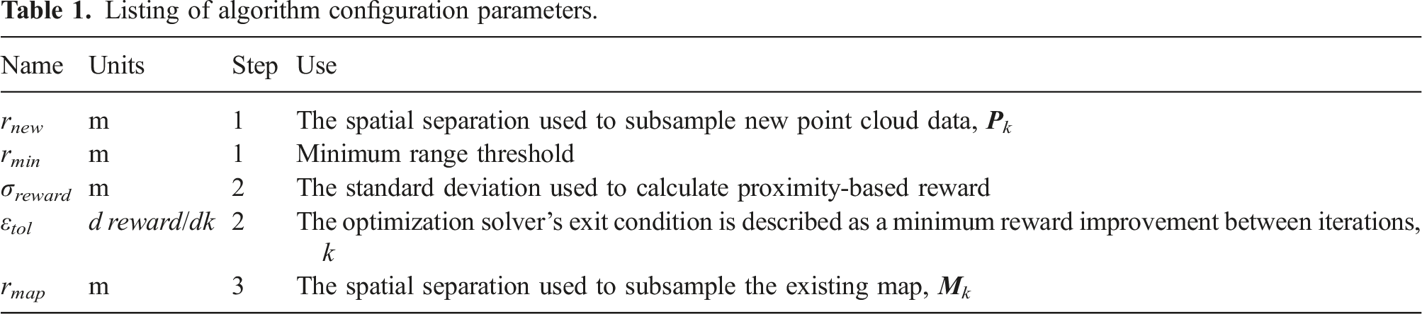
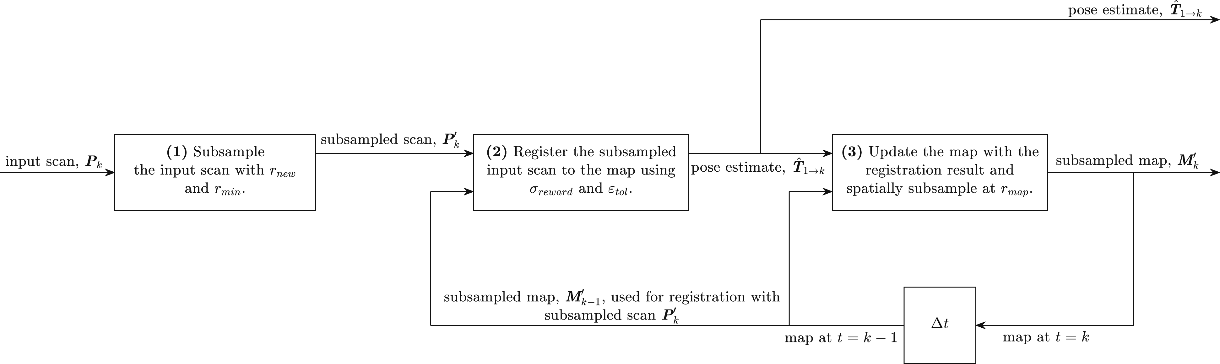
The SiMpLE algorithm consists of three steps and five configuration parameters. A new scan is first spatially subsampled before being registered against the incrementally generated map. The result provides the current pose estimate, which is directly used to update the map for the next registration result.

Algorithm 1: SiMpLE.

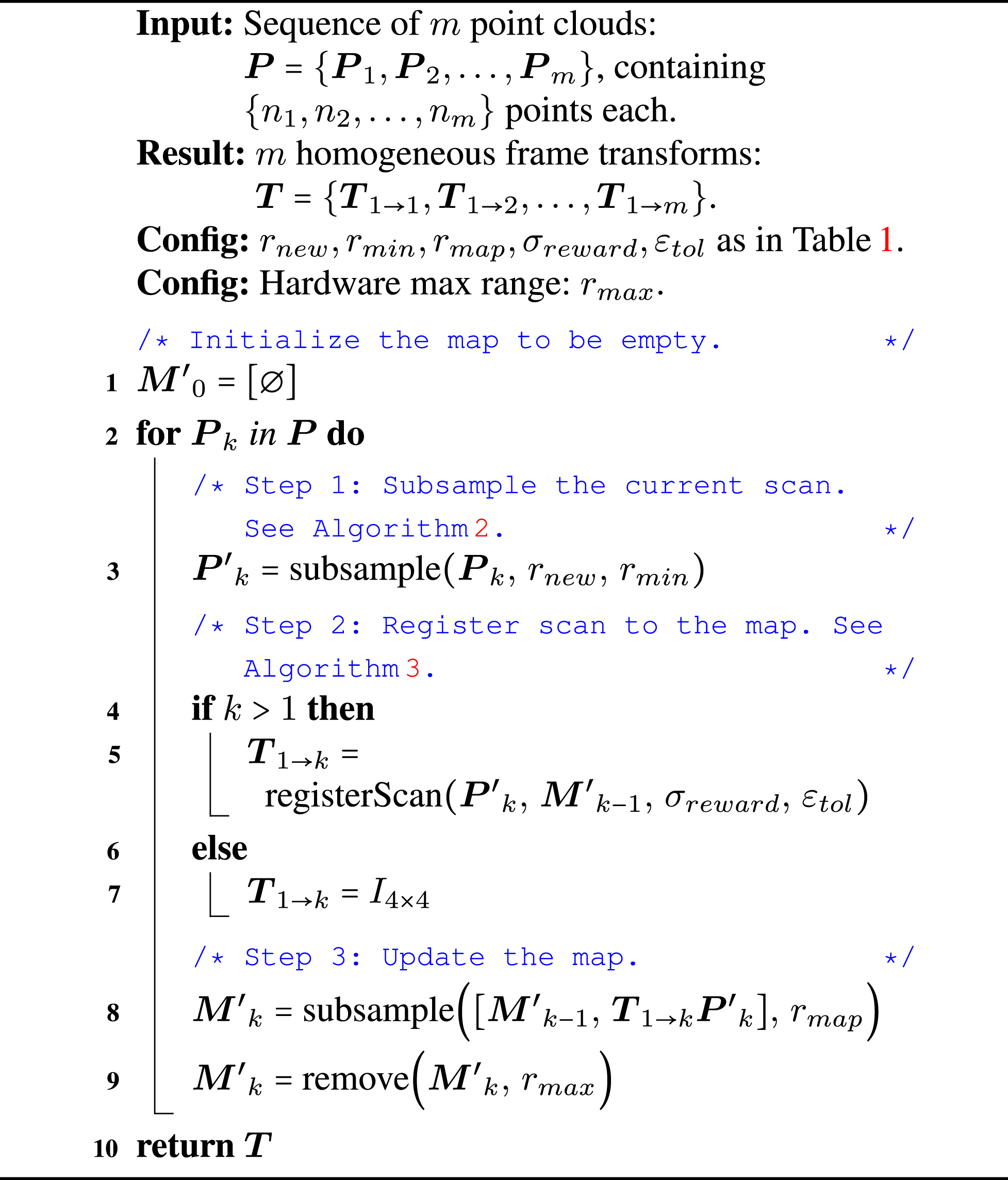
The SiMpLE algorithm contributes to providing a minimal configuration objective function. It is important to make a distinction between algorithm parameters that are configured upon general use (as displayed in Table 1), and those for which we use default values which are introduced by using open-source libraries. The five algorithm configuration parameters listed in Table 1 stem from the design of the SiMpLE algorithm.

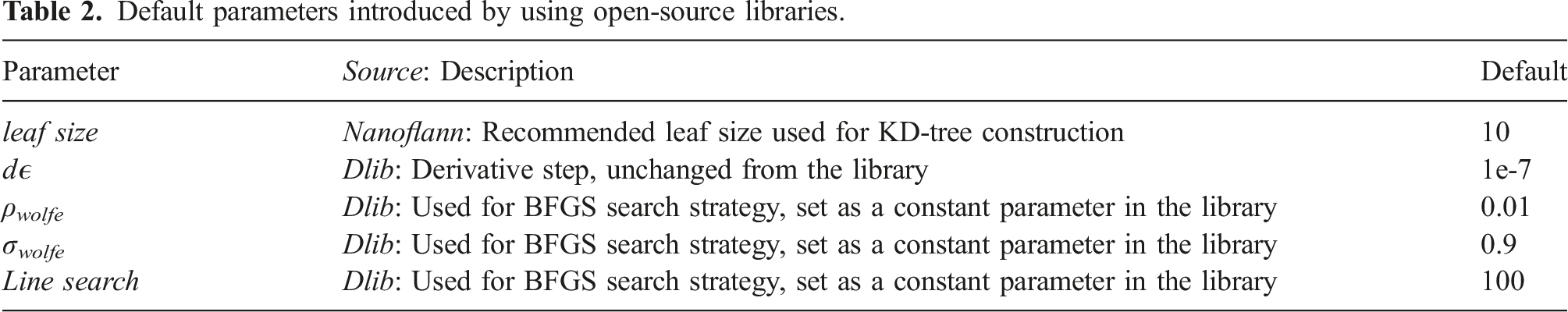
There are also other parameters introduced in the implementation from the nanoflann library (Blanco and Rai, 2014) used for nearest neighbour searches, and the Dlib optimization library (King, 2009) used for searching for the highest-scoring scan-to-map registration result. We use default values for parameters present in these libraries and leave them unchanged. For example, we use the recommended KD-tree leaf size of 10 as it allows for fast nearest point queries and do not change this throughout the evaluation. Similarly, the optimization solver has fixed search-specific parameters for the BFGS Quasi-Newton implementation described by Nocedal and Wright (1999). These parameters have nominal values and are hardcoded in the Dlib library. As the open-source library parameters are not configured upon using SiMpLE, we do not account for them in the algorithm’s configuration parameter count. This allows for a direct comparison of configuration parameters with existing approaches as well.

SiMpLE has been extensively tested on various benchmark datasets without altering the default parameters contained within the libraries used. The parameters introduced by libraries are listed in Table 2, and on the open-source page for complete transparency.

Table 2.

Default parameters introduced by using open-source libraries.

Parameter	Source: Description	Default
leaf size	Nanoflann: Recommended leaf size used for KD-tree construction	10
dϵ	Dlib: Derivative step, unchanged from the library	1e-7
ρ _wolfe	Dlib: Used for BFGS search strategy, set as a constant parameter in the library	0.01
σ _wolfe	Dlib: Used for BFGS search strategy, set as a constant parameter in the library	0.9
Line search	Dlib: Used for BFGS search strategy, set as a constant parameter in the library	100

5. Results

The results demonstrate the performance of the SiMpLE algorithm in comparison to other state-of-the-art LiDAR odometry methods using various case studies. The results demonstrate accurate localization with significantly less configuration than other methods. The KITTI, MulRan, UrbanNav, and a dataset recorded at the University of Queensland (UQ) are used to evaluate SiMpLE’s performance. Each dataset is recorded using a different sensor in dynamically changing environments. Figure 5 displays example scans from the datasets.

Figure 5.

Example scans from the evaluation datasets have varying densities and fields of view. The examples include a Velodyne HDL-64 scan from the KITTI dataset (top left), an Ouster OS1-64 scan from the MulRan dataset (top right), a Velodyne VLP-16 scan from the self-recorded dataset (bottom left), and a Livox Horizon scan (bottom right) from the self-recorded dataset. The axes display the origin of the sensor.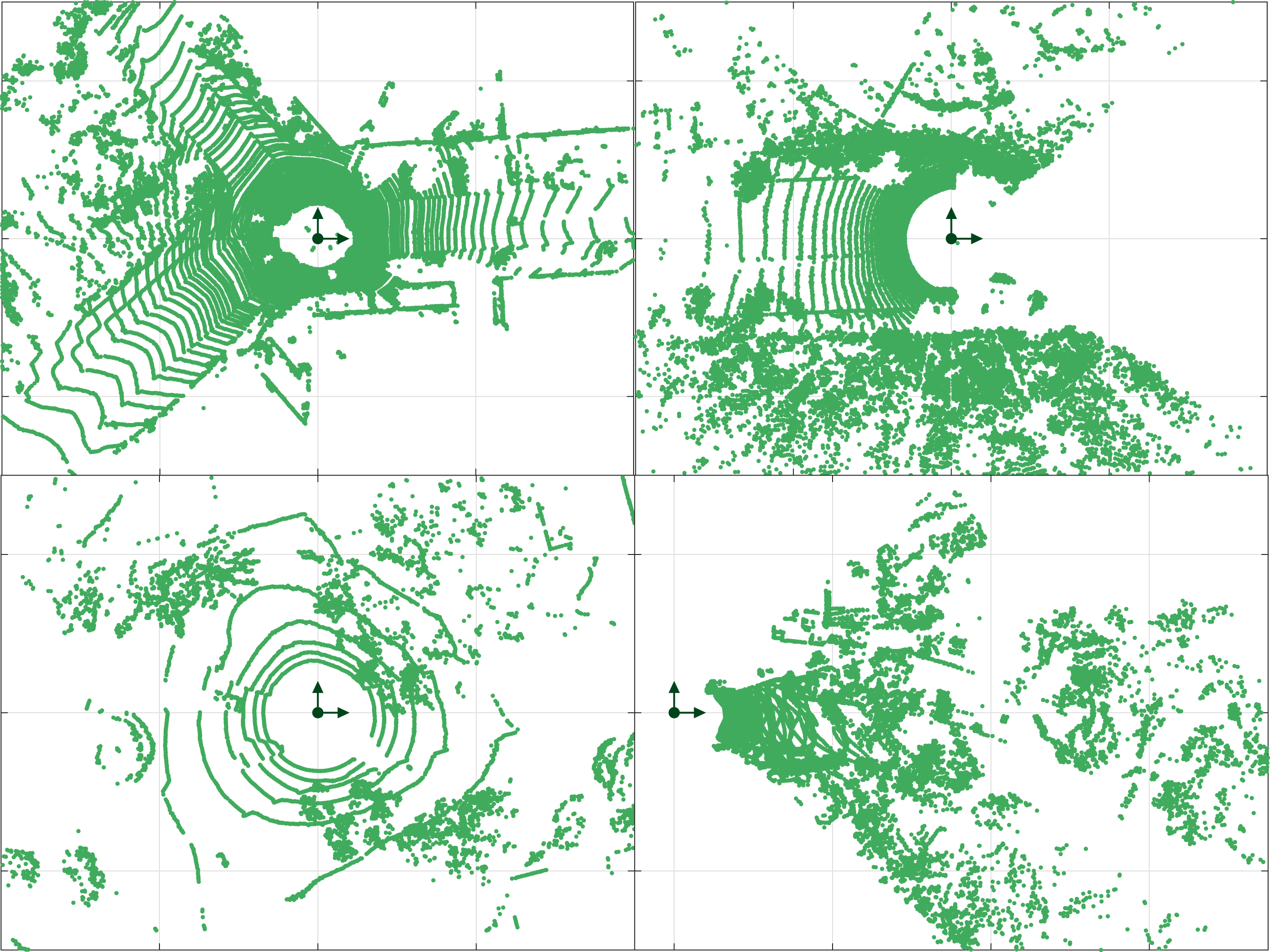

The KITTI dataset uses a Velodyne HDL-64E, providing dense point clouds with more than 100,000 points per scan on average. The Ouster OS1-64 in the MulRan dataset outputs 65,536 measurements per scan and has a 70-degree blind spot due to the placement of the sensor in front of a radar. The UQ dataset consists of a Velodyne VLP-16 providing low-density point clouds with 30,000 points per scan, and a Livox Horizon providing 48,000 points per scan at 10 Hz with a limited field of view.

Case study 1 (KITTI) uses the provided deskewed scans from the dataset for direct comparison with other methods. All other case studies use the raw point clouds to estimate the trajectory. The point clouds can be deskewed using a timestamped IMU or a constant velocity model as a pre-processing step and require knowledge about the sensor characteristics such as the timestamped beam firing sequence. The result can be used directly with SiMpLE.

The results presented below use a BFGS Quasi-Newton optimization solver, implemented using the open-source Dlib library by King (2009). The initial condition or seed for each optimization problem is estimated using the constant velocity model and the previous pose estimate as detailed in Section 4.2. The closest point search is computed using a KD-tree implementation from the open-source nanoflann library by Blanco and Rai (2014). All testing is performed using an Intel i7 CPU @ 3.80 GHz with 62.5 GiB memory running Ubuntu 20.04.5 LTS, and the results are computed using CPU threading only, implemented using Intel’s open-source Thread Building Blocks API (Intel, 2023). KITTI’s evaluation metric is used for reporting translational and rotational errors for the KITTI and MulRan datasets for direct comparison with other published methods. The evaluation metric is detailed in Geiger et al. (2012). All tests use (r_new, r_map, ɛ_tol) = (0.5, 2, 10⁻³). Hardware configures r_max while σ_reward depends on point cloud density. All results are reproducible using the provided code.

5.1. Case study 1: KITTI dataset

The KITTI training dataset is a benchmark for algorithm performance and consists of 11 sequences of urban, highway, and country environments with varying difficulty concerning path length, vehicle speed, and localization features. SiMpLE uses only the Velodyne HDL-64E scans to generate a trajectory estimate. A calibration factor is applied to the KITTI scans to account for intrinsic errors identified by Deschaud (2018).

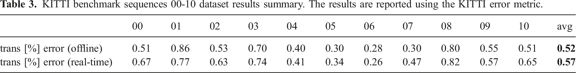
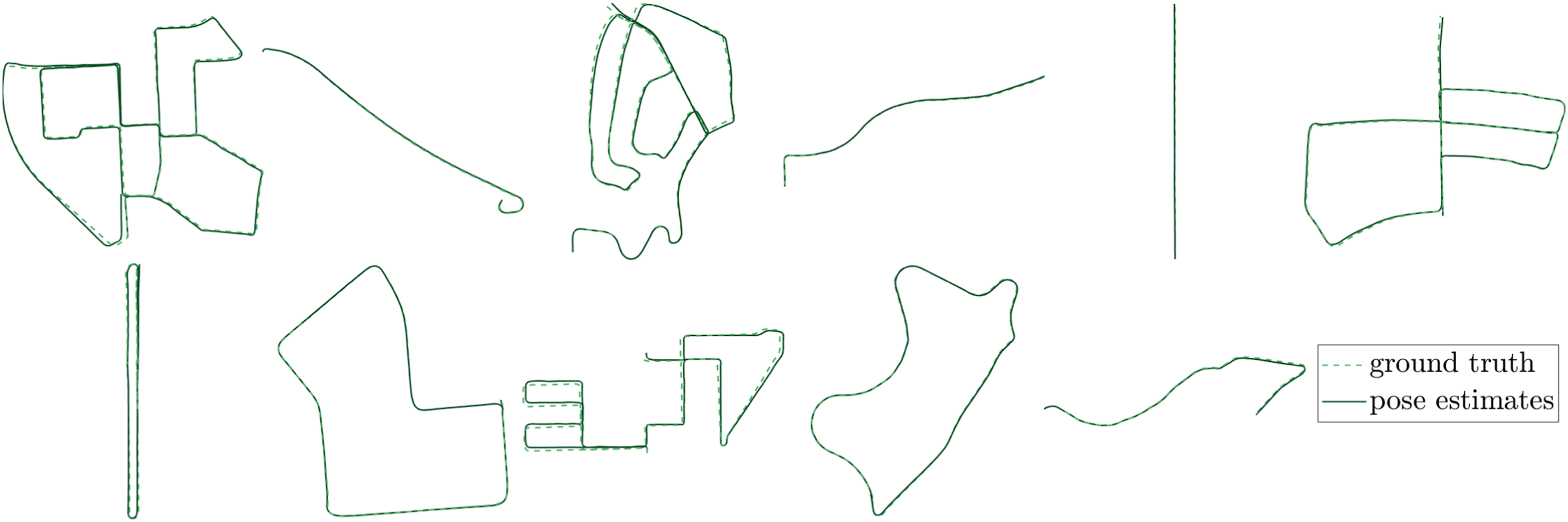
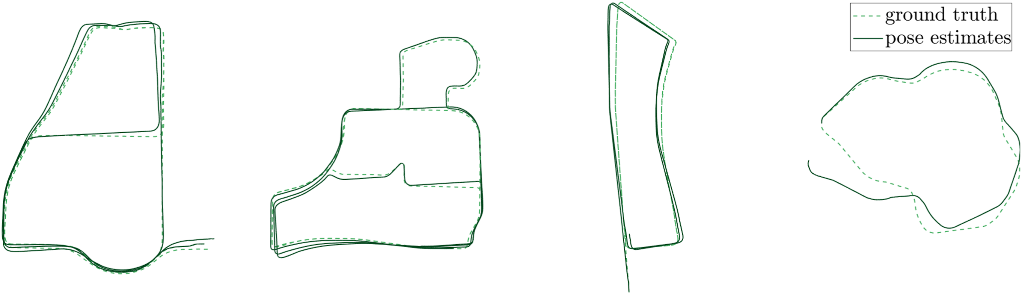
The performance of SiMpLE in comparison to other published methods is displayed in Figure 6, with the average translational error for each sequence listed in Table 3, evaluated using the KITTI metric for each sequence. Similar performance is achieved in comparison to state-of-the-art LiDAR odometry and loop closure methods at a significantly lower configuration burden. We outperform many sophisticated loop closure methods such as S4-SLAM by Zhou et al. (2021), and deep learning-based methods such as LoDoNet by Zheng et al. (2020) and LO-Net by Li et al. (2019). These methods are of higher fidelity and require training sets in some instances. Improved performance is achieved compared to state-of-the-art LiDAR odometry methods such as LOAM by Zhang and Singh (2014) and F-LOAM by Wang et al. (2021). Figure 7 displays a comparison between the ground truth and pose estimates for sequences 00-10. We achieve a mean translational and rotational error of 0.52% and 0.0013 deg/m offline and 0.57% and 0.0023 deg/m in real-time for the training dataset evaluated using KITTI’s metric. All tests use σ_reward = 0.3 m for the high point cloud density.

Figure 6.

An extensive comparison between LiDAR odometry methods utilizing a variety of techniques including point cloud registration, pose graph, feature extraction, semantic understanding, and deep learning. SiMpLE performs among the top-ranked LiDAR odometry methods (left). We use only front-end point cloud registration and perform similarly to the majority of the LiDAR odometry methods, with an average translational error of 0.52% offline and 0.57% in real-time, evaluated using KITTI’s provided metric. The results for the other methods are taken as published in Pan et al. (2021), Vizzo et al. (2023), and Kovalenko et al. (2019). SiMpLE outperforms state-of-the-art LiDAR odometry methods in the MulRan dataset’s four scenarios (right). Each scenario consists of three sequences, whose results have been averaged and presented. The results for the other methods are obtained from Vizzo et al. (2023).

Table 3.

KITTI benchmark sequences 00-10 dataset results summary. The results are reported using the KITTI error metric.

	00	01	02	03	04	05	06	07	08	09	10	avg
trans [%] error (offline)	0.51	0.86	0.53	0.70	0.40	0.30	0.28	0.30	0.80	0.55	0.51	0.52
trans [%] error (real-time)	0.67	0.77	0.63	0.74	0.41	0.34	0.26	0.47	0.82	0.57	0.65	0.57

Figure 7.

SiMpLE’s pose estimation results for KITTI sequences 00-10, consisting of 23,201 scans over 22.17 km. All sequences exhibit low drift using front-end LiDAR odometry only.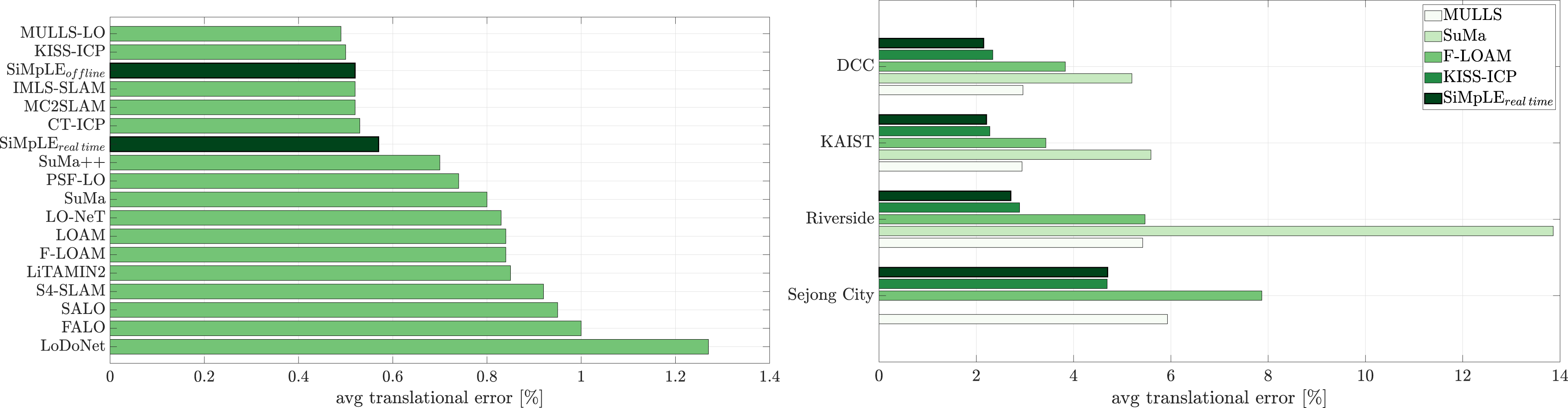

5.2. Case study 2: MulRan dataset

The recently introduced MulRan dataset by Kim et al. (2020) provides 12 challenging sequences in urban environments with corresponding ground truths. The sequences are considerably larger than KITTI in length and provide a greater structural and temporal diversity by being recorded at different locations and times of the year. Point clouds are obtained from a 64-beam Ouster OS1 LiDAR and are provided in the same format as the KITTI dataset. A challenging aspect of the dataset is the 70-degree blind spot in the LiDAR’s field of view due to the location of the radar. LiDAR odometry methods relying on point cloud registration suffer from incomplete scans.

Figure 6 displays the average translational error for the four test scenarios, with each scenario consisting of three sequences. The average translational error for each sequence is listed in Table 4, evaluated using the KITTI metric. We outperform top-ranked LiDAR odometry methods including MULLS, SuMa, F-LOAM, and KISS-ICP. The results for the other methods are taken as published in Vizzo et al. (2023). The strength of SiMpLE is in its reward-based metric, rewarding points that support the hypothesis only, and there is no assumption about the correspondence between points in successive scans. Some trajectory results are displayed in Figure 8. The most significant error is the drift in the z-axis due to the absence of a back-end. All tests use σ_reward = 0.35 m.

Table 4.

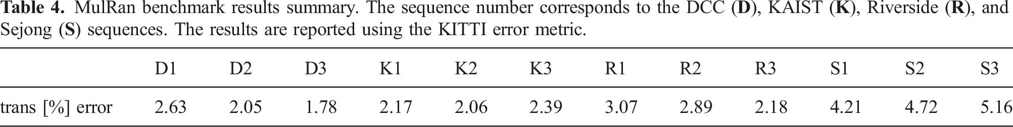
MulRan benchmark results summary. The sequence number corresponds to the DCC (D), KAIST (K), Riverside (R), and Sejong (S) sequences. The results are reported using the KITTI error metric.

	D1	D2	D3	K1	K2	K3	R1	R2	R3	S1	S2	S3
trans [%] error	2.63	2.05	1.78	2.17	2.06	2.39	3.07	2.89	2.18	4.21	4.72	5.16

Figure 8.

Example of pose estimation results from the MulRan dataset using SiMpLE for sequences (left to right) DCC (4.9 km), KAIST (6.1 km), Riverside (6.8 km), and Sejong (23.4 km). The complete 12 sequences consist of 154,035 scans over an approximate distance of 123.6 km, hence the increasing drift over longer distances using front-end LiDAR odometry only.

5.3. Case study 3: UrbanNav Dataset

The UrbanNav dataset by Hsu et al. (2021) provides a series of challenging datasets in so-called, urban canyons. The dataset focuses on the most challenging aspects of LiDAR odometry, including the presence of numerous dynamic objects and complex environmental structures. Huang et al. (2022) recently evaluated 7 point-wise and 5 feature-wise LiDAR odometry methods on two sequences from the dataset, namely, HK-Data20200314 (Data1) and HK-Data20190428 (Data2). Data1 is a small 1.21 km loop around a low-urbanization area, whereas Data2 is a 2.01 km loop in heavy traffic and tall buildings. SiMpLE outperforms all methods tested in Huang et al. (2022) with the results shown in Table 5 and Figure 9. The top two results for each dataset are listed here for comparison. For a fair comparison, the results are matched with the 1 Hz ground truth provided and evaluated using the EVO tools by Grupp (2017) to replicate the original testing conditions. All tests use σ_reward = 0.35 m.

Table 5.

SiMpLE UrbanNav results for Data1 and Data2.

		Trans. [m]		Rot. [deg]
Seq.	Method	RMSE	mean	RMSE	mean
Data1	SiMpLE	0.26	0.24	1.18	0.85
	G-ICP	0.37	0.33	1.91	1.27
	LOAM	0.35	0.31	2.11	1.38
Data2	SiMpLE	0.24	0.17	0.51	0.30
	G-ICP	0.42	0.30	1.13	0.66
	Fast LOAM	0.42	0.29	1.14	0.62

Figure 9.

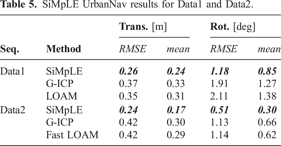
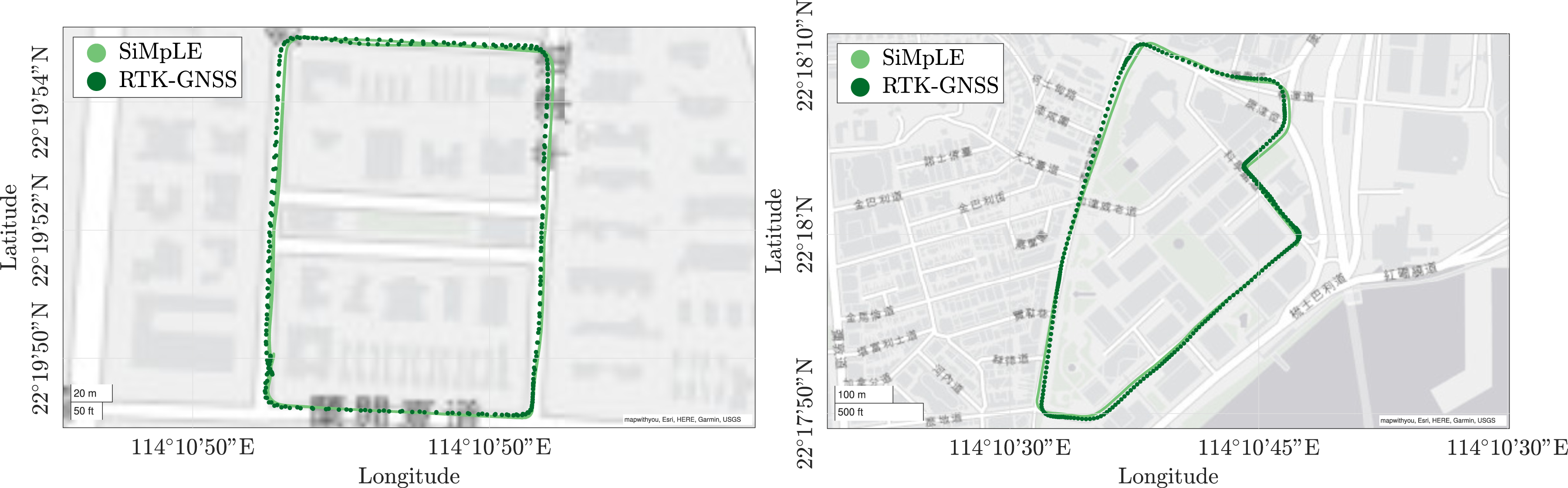
UrbanNav trajectory estimates for Data1 (left) and Data2 (right). SiMpLE experiences low drift in highly dynamic urban canyons. Loop closure methods can be employed with SiMpLE for better localization accuracy at the expense of increasing the configuration set.

5.4. Case study 4: The University of Queensland (UQ) St Lucia Campus

The KITTI, MulRan, and UrbanNav datasets provide high-density point clouds. To test SiMpLE’s performance with a different field of view and low-density point clouds, a vehicle was mounted with a Livox Horizon (Livox, 2019), a KAARTA Stencil 2 (KAARTA, 2021) using a Velodyne VLP-16, and a NovAtel navigation solution as displayed in Figure 10.

Figure 10.

The designed testing platform consists of a Livox Horizon, KAARTA Stencil 2, Velodyne VLP-16 LiDAR, and a NovAtel navigation solution.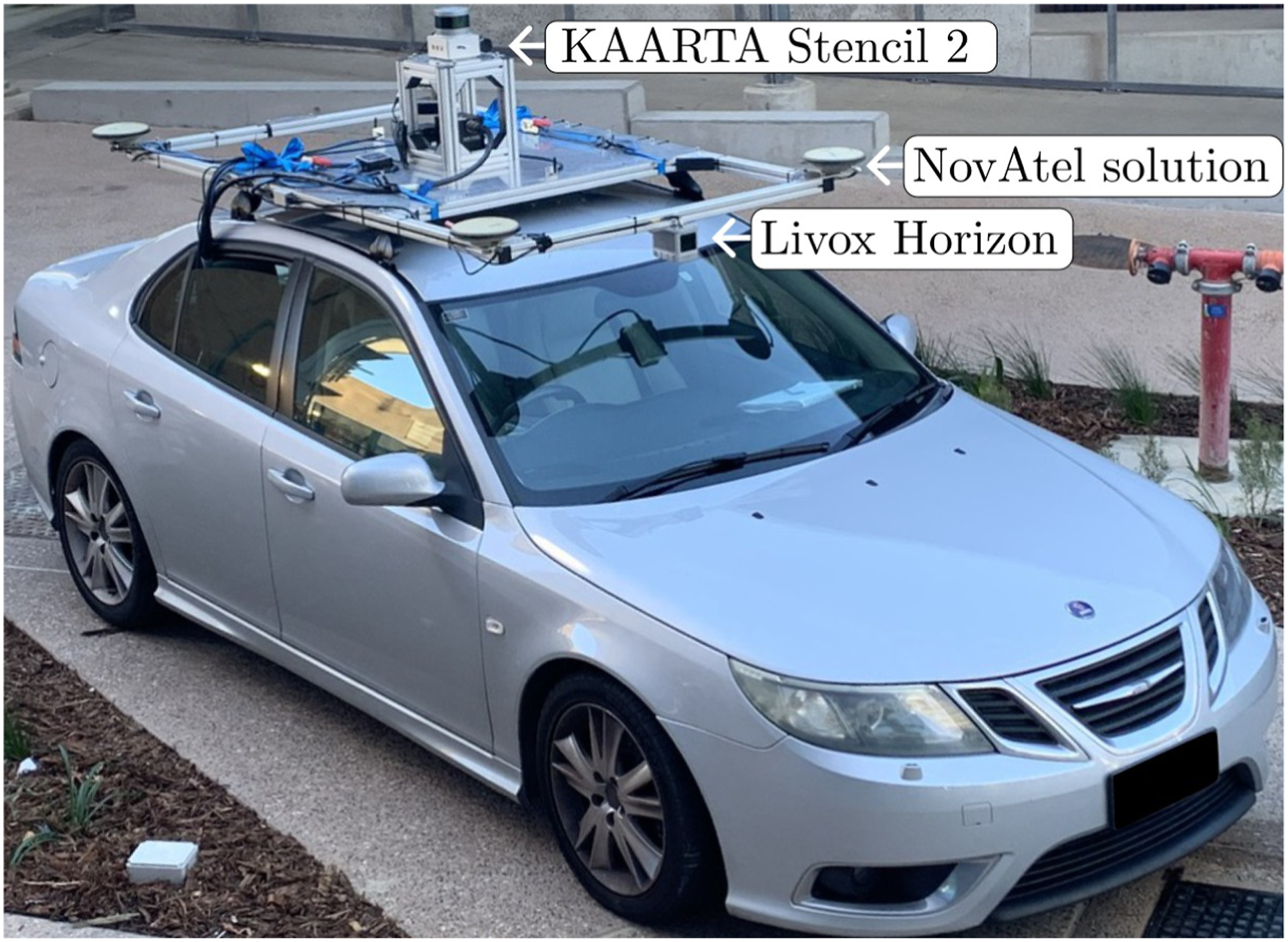

Table 6 details the datasets collected around the University of Queensland St Lucia campus. Due to the testing environment surrounded by trees, the RTK-GNSS ground truth was intermittently lost. SiMpLE’s performance is overlaid on a map of the environment along with the ground truth for evaluating the overall performance.

Table 6.

Self-recorded sequences.

Sequence	Sensor	Num. scans
UQ St Lucia campus loop	VLP-16	12,000
UQ ferry terminal to Boomerang Rd	Livox	2632
Guyatt Park to Building 45 UQ	Livox	2398

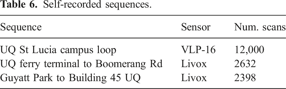
Figure 11 displays the results for a large dynamic sequence of 12,000 VLP-16 scans at 10 Hz recorded in the presence of other vehicles and pedestrians. The environment is mostly static with substantial vegetation alongside the road. Multiple closed loops are provided to aid the KAARTA SLAM solution. Using the raw VLP-16 scans only, SiMpLE adequately tracks the vehicle position and accumulates low drift over the entire sequence. The KAARTA solution with and without loop closure accumulates more drift and is unable to provide a reasonable trajectory. The large error in the KAARTA closed-loop trajectory may exist due to incorrect loop closure identification, offsetting the entire trajectory. SiMpLE only has five parameters, whereas the performance of the KAARTA solution is affected by up to 73 parameters (KAARTA, 2020). Further tuning the KAARTA parameters may result in a better trajectory. Figure 12 displays the pose estimation results for two sequences consisting of 2600 and 2300 scans each recorded using the Livox Horizon LiDAR. This dataset is included to show SiMpLE’s performance with a LiDAR with a different field of view and scan pattern. Low drift is accumulated along the entire sequence.

Figure 11.

Trajectory estimate results around the University of Queensland St Lucia campus generated from 12,000 Velodyne VLP-16 scans at 10 Hz. SiMpLE (left) accumulates low drift over the entire sequence using front-end odometry only. Decreasing the subsampling from r_new = 0.5 m to r_new = 0.25 m allows for highly accurate localization. The KAARTA front-end odometry (middle) and KAARTA SLAM (right) solutions drift significantly over time and may be corrected by tuning the configuration parameters. The GNSS solution drops out on multiple occasions due to loss of signal in paths with significant vegetation cover.

Figure 12.

The SiMpLE odometry results (left) for two sequences recorded using a Livox Horizon mounted at the front of the vehicle. SiMpLE accurately tracks the vehicle position with low accumulated drift. A sample scan from the Livox LiDAR is shown on the right (the full scan is not shown due to the sparsity at long range). The field of view and scan pattern is different compared to a mechanical rotating LiDAR such as the Velodyne VLP-16. The scan shows parked vehicles, the road, and an overhead bridge, with the point colour indicating the return intensity.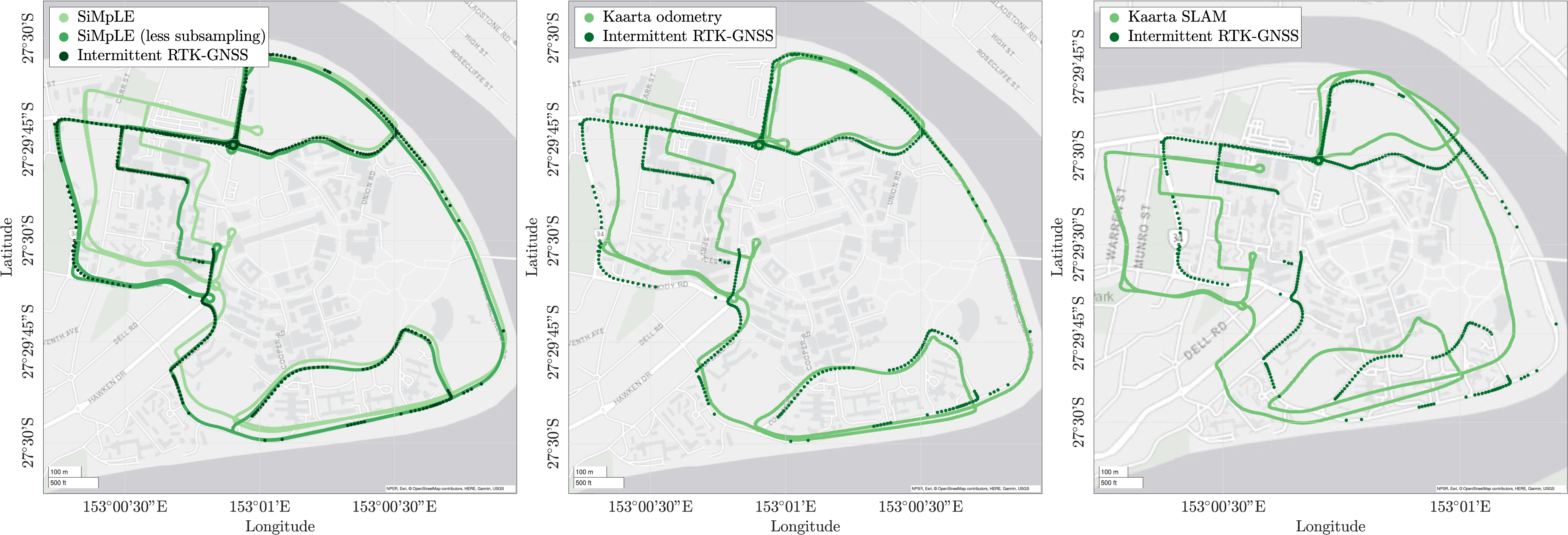

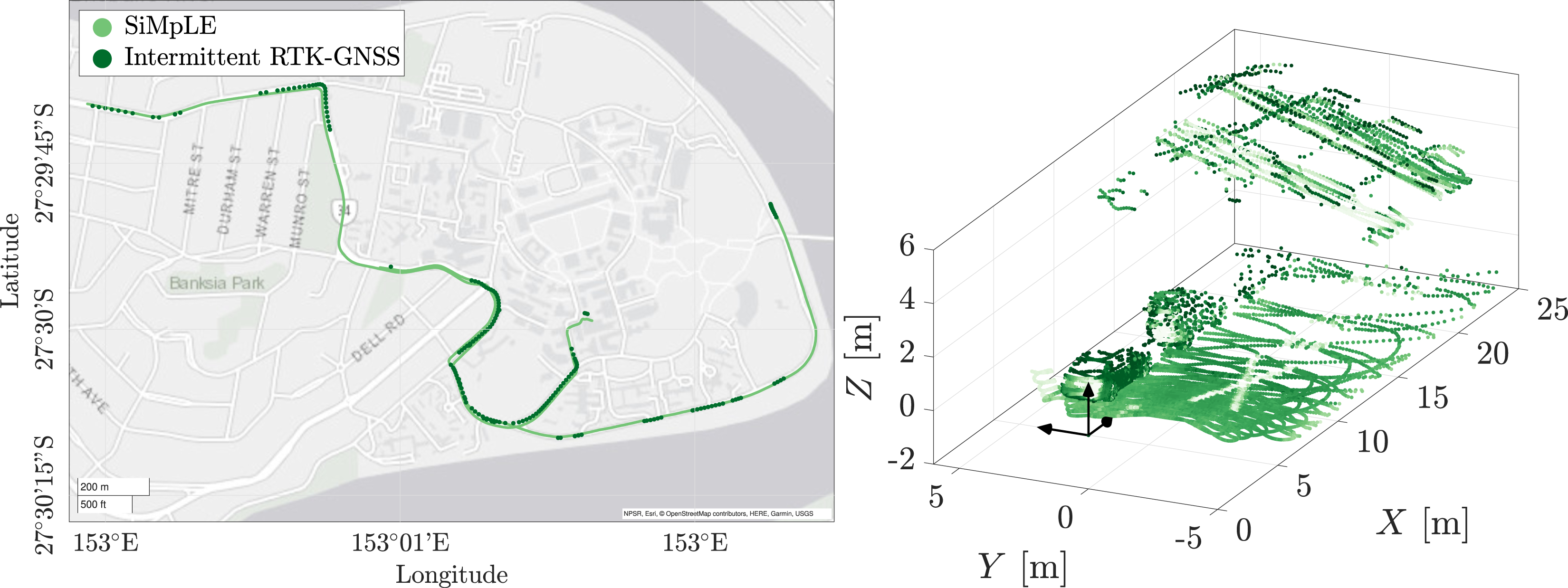
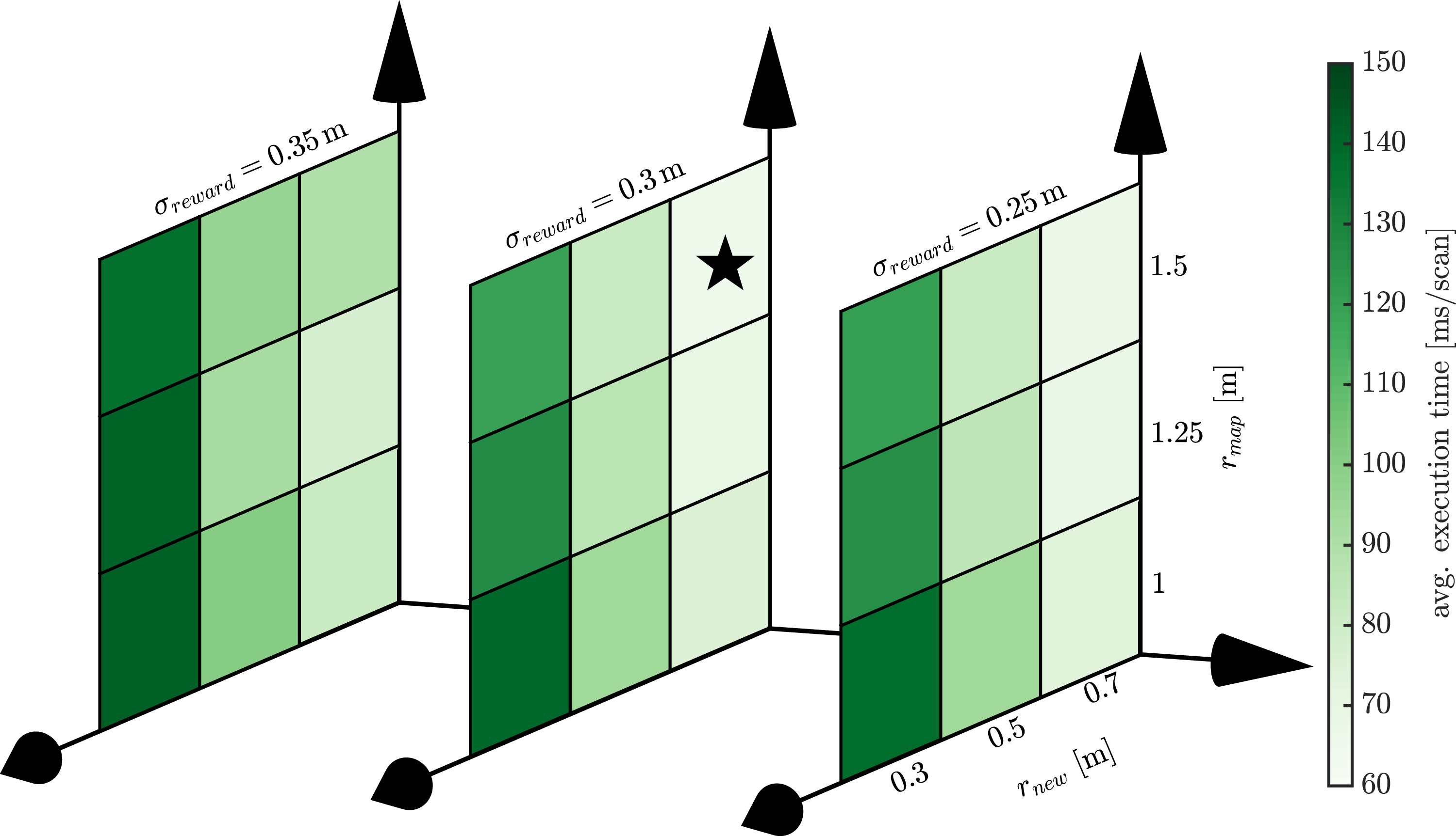
5.5. Parameter sensitivity

SiMpLE has five configuration parameters. Along with limiting the possible permutation of configuration parameters, the parameters should be insensitive to small deviations for applicability in different environments and point cloud characteristics such as the scan pattern and point cloud density. Many methods rely on fine-tuning the configuration parameters for optimal performance. Figure 13 displays the average translational error for KITTI sequences 00-10 across 27 permutations of the input parameters; r_new, r_map, and σ_reward. Similar results are obtained regardless of the configuration, with a low standard deviation of 0.07% translational error. Real-time pose estimation demands a generic set of parameters that do not require post-processing tuning. For optimal performance, the input scan subsampling, r_new, should be as small as possible to provide an accurate representation of the environment. This is limited by the computational resources, as each point in the input scan is rewarded when evaluating the objective function. The algorithm needs to provide pose estimates commensurate with the required rate of control decisions. The size of the map depends on the subsampling radius, r_map, and is generally set to be larger than r_new to overcome the effect of the sensor’s scan pattern. The registration reward, σ_reward, is shown to be insensitive above, and is generally set to a value similar to the input scan subsampling, r_new.

Figure 13.

SiMpLE’s configuration parameters are insensitive to small changes. The heatmaps demonstrate minimal changes in the translational error results for the KITTI training dataset over 27 permutations of the configuration parameters, r_new, r_map, and σ_reward. The best result is indicated with a star. Only having three main configuration parameters allows for visualization of the configuration space. This is not possible for the majority of LiDAR odometry methods.

5.6. Real-time performance

The pose estimation evaluation time for SiMpLE is affected by the subsampling radii r_new and r_map, and the optimization convergence criterion, ɛ_tol. Larger scans take longer to spatially subsample, and scans subsampled at a small radius, r_new, result in a larger number of Cartesian points that need to be rewarded per objective function evaluation, consequently requiring greater computation time as demonstrated in Table 7. A small map subsampling radius, r_map, results in a larger size of the map, requiring more time to build and then search the KD-tree for the closest points in the objective function. Setting a smaller convergence tolerance for the optimization solver requires more evaluations of the objective function, increasing computation time at the expense of increased accuracy. Figure 14 visualizes the relationship between the configuration parameters on the average execution time for the KITTI dataset.

Table 7.

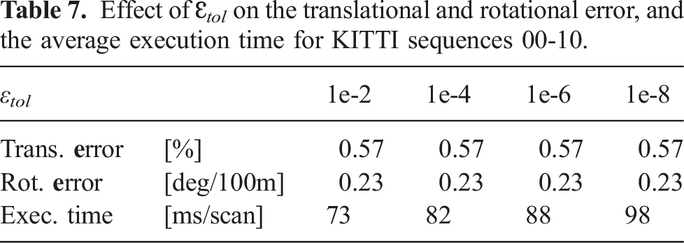
Effect of Ɛ_tol on the translational and rotational error, and the average execution time for KITTI sequences 00-10.

ɛ _tol		1e-2	1e-4	1e-6	1e-8
Trans. error	[%]	0.57	0.57	0.57	0.57
Rot. error	[deg/100m]	0.23	0.23	0.23	0.23
Exec. time	[ms/scan]	73	82	88	98

Figure 14.

The average execution time per scan is proportional to the size of the point cloud being scored in the objective function. A smaller subsampling radius preserves the geometrical features of the point cloud and results in higher accuracy as illustrated in Figure 13, but results in a greater execution time as illustrated here. This is severely impacted by the size of the original point cloud. For example, the KITTI point clouds are double in size compared to the MulRan dataset. The results are demonstrated using the KITTI training dataset with the star indicating the fastest average evaluation time.

The results for the KITTI, MulRan, and the UQ datasets all provide real-time results at a minimum of 10 Hz to match the sensor frame rate as displayed in Table 8. The MulRan dataset consists of 65,536 points per scan, compared to the KITTI dataset containing over 100,000 points per scan. This results in a larger spatial subsampling and objective function evaluation time for the KITTI dataset. The parameters can be adjusted to increase subsampling with minimal effect on the registration accuracy as shown previously. The Velodyne VLP-16 scans are much smaller, with approximately 10,000 points per scan.

Table 8.

Average SiMpLE processing times.

Dataset	Approx. scan size [pts]	Time/scan [ms]
KITTI	122,186	75
MulRan	65,536	70
UrbanNav	63,362	68
UQ VLP-16	23,107	36
UQ Livox	48,000	52

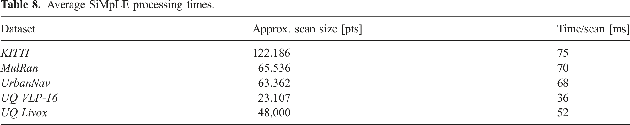
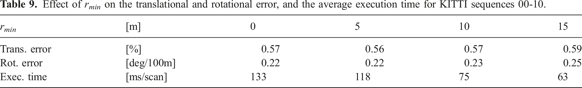
An optional parameter, r_min, may be used to reduce the number of points per scan and allow for real-time applicability when using a small subsampling radius. Scan points with a range of less than r_min are discarded. Figure 15 displays the effect of applying r_min to a scan, and Table 9 displays the effect of r_min on the algorithm performance. We emphasize this is optional and for computational benefit only. The r_min parameter can be disregarded given adequate computational resources. The MulRan and self-recorded dataset provides real-time pose estimates using the default value of r_min = 0 m.

Figure 15.

The original scan with 124,668 points using the default r_min = 0 m (left). The same scan with 62,304 points using r_min = 10 m. The scan properties and features are preserved with only the inner rings removed. This reduces the point cloud size by approximately 50%, allowing for faster objective function evaluations.

Table 9.

Effect of r_min on the translational and rotational error, and the average execution time for KITTI sequences 00-10.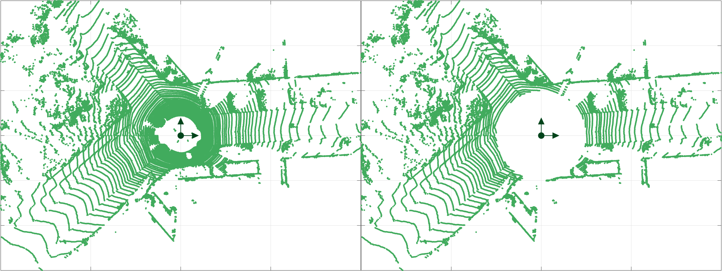

r _min	[m]	0	5	10	15
Trans. error	[%]	0.57	0.56	0.57	0.59
Rot. error	[deg/100m]	0.22	0.22	0.23	0.25
Exec. time	[ms/scan]	133	118	75	63

The real-time performance depends strongly on the ability to perform CPU threading. The objective function benefits immensely from the parallel computation of the independent per-point reward calculation. Common open-source threading APIs such as Intel’s Thread Building Blocks (TBBs) (Intel 2023) and OpenMP (OpenMP, 2023) allow for easy parallelization. We have tested with TBB on Intel and macOS ARM processors, and OpenMP is documented to support Intel, AMD, and ARM processors. TBB is used for our open-source implementation as our testing has demonstrated superior performance to OpenMP with automatic thread allocation.¹ The dependence on threading for real-time performance is depicted in Figure 16, along with a comparison of TBB vs OpenMP for our specific task. We use TBB as it performs automatic thread allocation and provides a greater than three times faster evaluation of the objective function.

Figure 16.

SiMpLE’s real-time performance relies on the ability to thread the objective function evaluation. The plot shows the effect of increasing the number of threads on the average execution time, with the real-time results indicated in a darker colour. The threads are set manually using OpenMP, with TBB having automatic thread allocation. Threading allows for the average execution time to decrease from approximately 250 ms to 75 ms, a greater than three times speed benefit. The error bars show the standard deviation of the timing results, with the execution time varying with the density of the point cloud. All results presented in this paper are executed in real-time using TBB.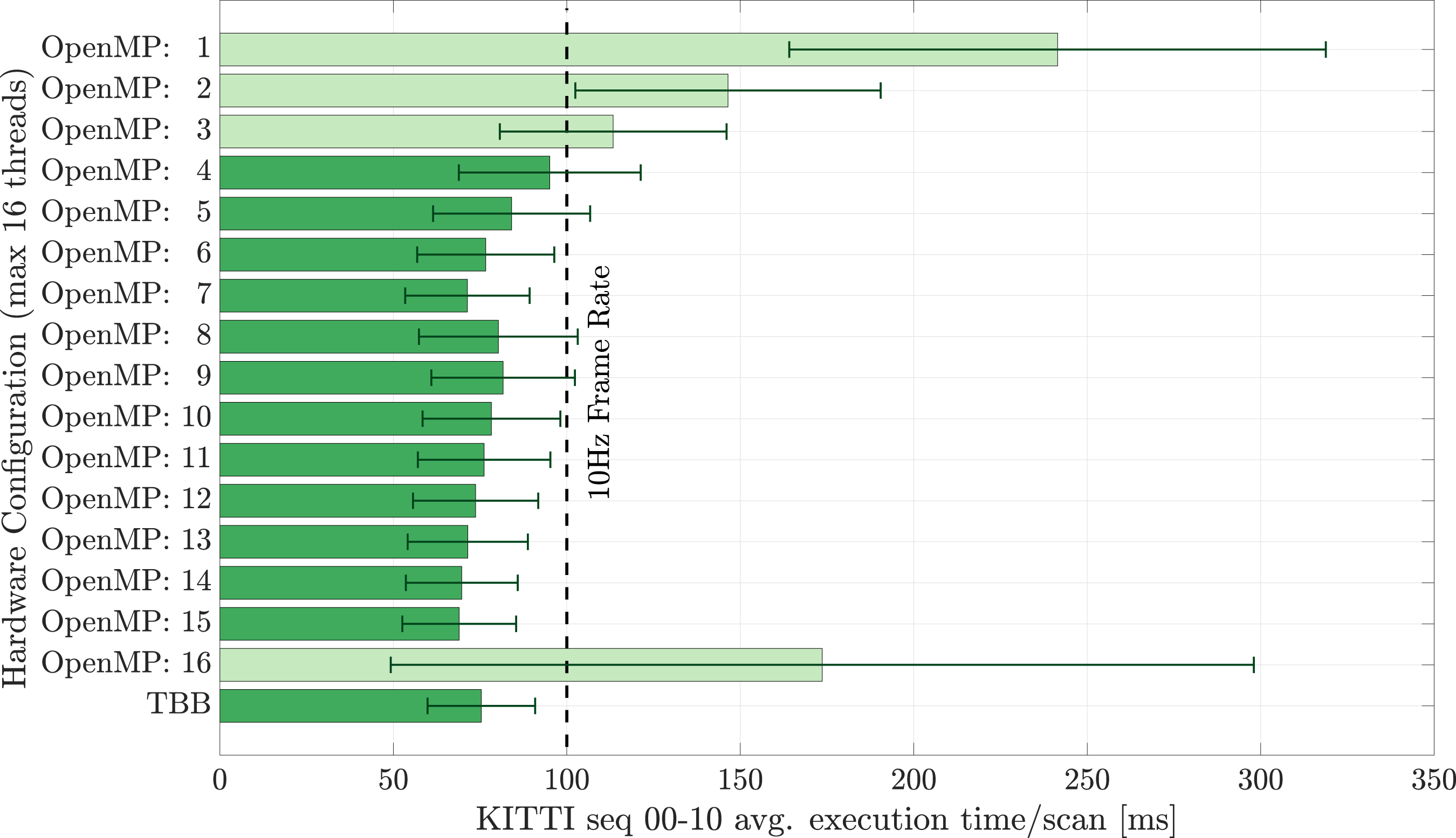

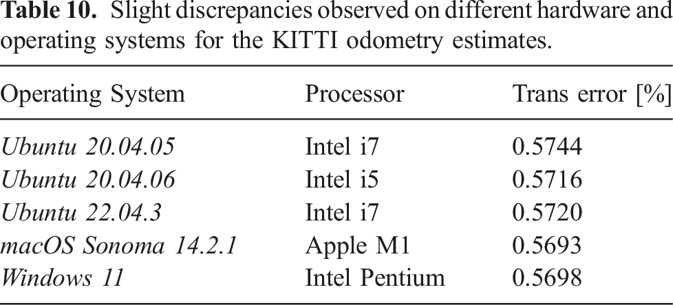
The implementation allows for deterministic results for a varying number of threads on a given platform, that is, executing a test with the same configuration given some number of threads allows for repeatable results on the same platform. However, we note slight discrepancies when testing the implementation across various CPUs and operating systems. Upon investigation, this is found to arise in Dlib’s optimization when searching for the best hypothesis. Specifically, this occurs in minute numerical precision differences in the step sizes used for searching around the seed. Due to the nature of recursive pose estimation, the differences propagate and result in slight variations in the output trajectory. Example results from the KITTI dataset executed on different operating systems and processors are displayed in Table 10. Only slight precision differences are present.

Table 10.

Slight discrepancies observed on different hardware and operating systems for the KITTI odometry estimates.

Operating System	Processor	Trans error [%]
Ubuntu 20.04.05	Intel i7	0.5744
Ubuntu 20.04.06	Intel i5	0.5716
Ubuntu 22.04.3	Intel i7	0.5720
macOS Sonoma 14.2.1	Apple M1	0.5693
Windows 11	Intel Pentium	0.5698

6. Future work

We propose SiMpLE as a fundamental work that provides a significant opportunity for development to achieve improved registration accuracy, speed, and robustness of localization methods. However, many of these occur at the cost of increasing the configuration set, detracting from the simplicity of SiMpLE. A few of the extensions are discussed below.

SiMpLE is a recursive pose estimator. The result at time k is dependent on the registration result at time k − 1. A single large registration error has the potential to offset the entire trajectory and a lack of back-end processing results in future estimates propagating the error. The integration of a constant velocity or constant acceleration process model with common filter-based state estimators such as a Kalman filter is expected to reduce the effect of erroneous registrations. The current implementation is agnostic to the dynamics of the mobile platform, but this prior information could be used to increase the accuracy of the results. However, this comes at the expense of adding configuration parameters in implementing the filter. A measure of uncertainty for the PC2PC registration process also needs to be derived as an input to the filter.

The filter can also be used to integrate information from other sensing modalities, such as GNSS, IMU, and vision-based approaches for increased robustness and redundancy. D’Adamo et al. (2022) formulated an Extended Kalman Filter to fuse information from a GNSS, IMU, and LiDAR to increase pose estimation accuracy and allow for 6-DOF pose estimation using two GNSS receivers only. An IMU can also be used directly in the SiMpLE algorithm as an alternative to the constant velocity model used to estimate the seed for the optimization solver. This is expected to allow for faster convergence to the optimal solution. LiDAR-inertial odometry has been vastly explored, with Wildcat by Ramezani et al. (2022) being a prominent example.

SiMpLE’s objective function uses a single configuration parameter, σ_reward. In this paper, σ_reward is selected arbitrarily and shown to be insensitive over a range of values. Currently, the scalar distance between two points is used in the Gaussian function as displayed in equation (1) and equation (5). This rewards distance errors in each axis, x, y, and z, equally. However, this may not be accurate when examining the shape of the point cloud, where there is different movement in each axis for a given mobile platform. For example, a car moves significantly more in the forward axis of a mobile vehicle than in other directions. Similar to NDT, σ_reward can be expanded to a 3 × 3 matrix to allow for scoring each axis separately and hence extending the equation (5) to a matrix operation.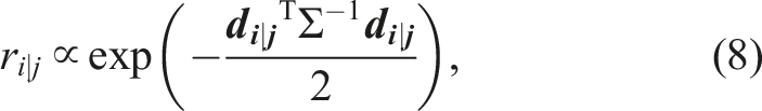

r_{i | j} \propto \exp (- \frac{{d_{i | j}}^{T} Σ^{- 1} d_{i | j}}{2}),

(8)

where d _i|j is a vector for the Cartesian distance between the points in each axis, and Σ is the scoring matrix,

Σ = [\begin{array}{l} σ_{x}^{2} & 0 & 0 \\ 0 & σ_{y}^{2} & 0 \\ 0 & 0 & σ_{z}^{2} \end{array}] .

(9)

We believe there is future work to automatically determine the value of Σ for optimal registration depending on the shape of the point cloud. This can help reduce another configuration parameter.

As mentioned previously, SiMpLE provides a front-end solution only. Back-end methods have been extensively explored as they have the potential to reduce accumulated drift. Due to the high portability of SiMpLE, it can be integrated directly with existing back-end solutions such as GTSAM by Dellaert and Kaess (2017) or g2o by Kümmerle et al. (2011). The results demonstrate that SiMpLE accumulates low drift over long sequences, aiding the pose graph methods.

SiMpLE uses CPU threading to accelerate the evaluation of the objective function. It is apparent that lower subsampling radii better preserve the structure of the scan and map; however, this leads to increased computation time and provides offline results. A GPU-based implementation can be explored to accelerate the execution with minimal subsampling.

7. Conclusion

The significant contribution of this paper is providing and demonstrating that a simple solution to the localization problem exhibits similar, if not better, results than most LiDAR odometry solutions available. The simple process of using scan-to-map registration with a reward-based metric provides robust pose estimation results. With the applications and use of SLAM in modern robotics growing exponentially, proposed solutions are increasing complexity to adapt to new challenges and consequently growing configuration parameters. While tuning guides are often prescribed, a user-friendly algorithm should limit the configuration permutations and the sensitivity of the parameters.

This paper derives a LiDAR odometry method from raw point cloud data, demonstrating real-time and highly accurate registration in a variety of scenarios with a minimal and low-sensitivity configuration set. SiMpLE has five configuration parameters; namely r_new and r_map for the subsampling of the input scan and map respectively, r_min for computational benefit, σ_reward for the scan-to-map registration, and ɛ_tol for the optimization search termination condition. All parameters are shown to be insensitive to small changes, providing similar results with various permutations.

SiMpLE is benchmarked using the 11 KITTI training sequences consisting of 23,201 Velodyne HDL-64E scans, 12 MulRan sequences consisting of 154,035 Ouster OS1–64 scans, and the UrbanNav dataset. SiMpLE outperforms top-ranked LiDAR odometry methods on all datasets. To test the proposed algorithm with low-density point clouds, a dataset was recorded at the University of Queensland using a Velodyne VLP-16 and Livox Horizon LiDAR and evaluated using a NovAtel ground truth. The SiMpLE solution outperforms the out-of-the-box KAARTA solution with and without loop closure.

SiMpLE is an easy-to-configure and use solution to the LiDAR odometry problem. The open-source code provided is extremely lightweight and written to match the layout of the paper. It easily integrates into existing projects with minimal dependencies. As explored in the previous section, SiMpLE provides a significant opportunity for improvement by augmenting the method with state estimators, other sensing modalities, and loop closure methods, all at the cost of expanding the configuration set. Using only five configuration parameters, the algorithm performs among top-ranked LiDAR odometry methods including MULLS, KISS-ICP, F-LOAM, and SuMa. This paper addresses the foundation of the LiDAR odometry problem only using scan-to-map registration.

Footnotes

Acknowledgements

The authors would like to thank the reviewers and editors for their constructive feedback.

Declaration of conflicting interests

The author(s) declared no potential conflicts of interest with respect to the research, authorship, and/or publication of this article.

Funding

The author(s) disclosed receipt of the following financial support for the research, authorship, and/or publication of this article: The first named author has been funded by the Research Training Program (RTP) provided by the Australian Commonwealth and administered by the University of Queensland.

ORCID iD

Vedant Bhandari

Note

Appendix

The algorithms for the spatial subsampling and objective function are summarized below.

References

Aeva (2022) Aeries 1: The First 4d lidar^TM System for Autonomy Aeva Inc. https://www.aeva.com/aeries-i/.

Behley

Stachniss

(2018) Efficient surfel-based slam using 3d laser range data in urban environments. In: Robotics: Science and Systems, Volume 2018. 59.

Bergelt

Khan

Hardt

(2017) Improving the intrinsic calibration of a Velodyne LiDAR sensor. In: Proceedings of IEEE Sensors, Scotland, UK, 2017-December, 1–3. DOI:10.1109/ICSENS.2017.8234357.

Besl

McKay

(1992) A method for registration of 3-d shapes. IEEE Transactions on Pattern Analysis and Machine Intelligence 14: 239–256. DOI: 10.1109/34.121791.

Bhandari

Phillips

McAree

(2023) Real-time 6-dof pose estimation of known geometries in point cloud data. Sensors 23(6): 23. DOI: 10.3390/s23063085.

Biber

Straßer

(2003) The normal distributions transform: a new approach to laser scan matching. In Proceedings 2003 IEEE/RSJ International Conference on Intelligent Robots and Systems (IROS 2003)(Cat. No. 033CH37453), 2003, Vol. 3, 2743–2748. DOI: 10.1109/IROS.2003.1249285.

Blanco

Rai

(2014) Nanoflann: a C++ Header-Only Fork of FLANN. a library for nearest neighbor (NN) with kd-trees. https://github.com/jlblancoc/nanoflann

Botev

Grotowski

Kroese

(2010) Kernel density estimation via diffusion. Annals of Statistics 38(5): 2916–2957. DOI: 10.1214/10-AOS799.

Cao

Mendoza

Philipp

, et al. (2021) Lidar-based object-level slam for autonomous vehicles. IEEE International Conference on Intelligent Robots and Systems, 2003, pp. 4397–4404. DOI: 10.1109/IROS51168.2021.9636299.

10.

Cartographer

(2022) Tuning Methodology. https://google-cartographer-ros.readthedocs.io/en/latest/tuning.html

11.

Chen

Milioto

Palazzolo

, et al. (2019) Suma++: efficient lidar-based semantic slam. In 2019 IEEE/RSJ International Conference on Intelligent Robots and Systems (IROS). 2019, pp. 4530–4537. DOI: 10.1109/IROS40897.2019.8967704.

12.

Chen

Tang

Feng

, et al. (2017b) Possibility of applying slam-aided lidar in deep space exploration. In 3rd International Symposium of Space Optical Instruments and Applications: Beijing, China June 26-29th 2016, 2017, pp. 239–248. DOI: 10.1007/978-3-319-49184-4_24.

13.

Chen

Wang

, et al. (2021) Psf-lo: parameterized semantic features based lidar odometry. In 2021 IEEE International Conference on Robotics and Automation (ICRA). 2021, pp. 5056–5062. DOI: 10.1109/ICRA48506.2021.9561554.

14.

Chen

Zhang

, et al. (2017a) Robust slam system based on monocular vision and lidar for robotic urban search and rescue. In SSRR 2017 - 15th IEEE International Symposium on Safety, Security and Rescue Robotics, Conference, 2017, pp. 41–47. DOI: 10.1109/SSRR.2017.8088138.

15.

Cheng

Chen

Liu

, et al. (2018) Registration of laser scanning point clouds: a review. Sensors 18(5): 1641. DOI:10.3390/S18051641.

16.

Clotet

Palacín

(2023) Slamicp library: accelerating obstacle detection in mobile robot navigation via outlier monitoring following icp localization. Sensors 23(15): 16. DOI: 10.3390/s23156841.

17.

Dellaert

Kaess

(2017) Factor Graphs for Robot Perception. Foundations and Trends in Robotics 6, URL https://www.cs.cmu.edu/∼kaess/pub/Dellaert17fnt.pdf

18.

Deschaud

(2018) Imls-slam: scan-to-model matching based on 3d data. In: 2018 IEEE International Conference on Robotics and Automation (ICRA). 2018, pp. 2480–2485. DOI:10.1109/ICRA.2018.8460653.

19.

Diosi

Taylor

Kleeman

(2005) Interactive slam using laser and advanced sonar. In: Proceedings of the 2005 IEEE International Conference on Robotics and Automation. 2005, pp. 1103–1108. DOI:10.1109/ROBOT.2005.1570263.

20.

Donoso

Austin

McAree

(2017) How do icp variants perform when used for scan matching terrain point clouds? Robotics and Autonomous Systems 87: 147–161. DOI: 10.1016/j.robot.2016.10.011.

21.

Durrant-Whyte

Bailey

(2006) Simultaneous localization and mapping: Part i. IEEE Robotics and Automation Magazine 13: 99–108. DOI: 10.1109/MRA.2006.1638022.

22.

D’Adamo

Phillips

McAree

(2018) Registration of three-dimensional scanning lidar sensors: an evaluation of model-based and model-free methods. Journal of Field Robotics 35: 1182–1200. DOI: 10.1002/ROB.21811.

23.

D’Adamo

Phillips

McAree

(2022) Lidar-stabilised gnss-imu platform pose tracking. Sensors 22(6): 2248. DOI: 10.3390/s22062248.

24.

Filipenko

Afanasyev

(2018) Comparison of various slam systems for mobile robot in an indoor environment. 9th International Conference on Intelligent Systems 2018: Theory, Research and Innovation in Applications, IS 2018 - Proceedings, 2018, pp. 400–407. DOI: 10.1109/IS.2018.8710464.

25.

Geiger

Lenz

Urtasun

(2012) Are we ready for autonomous driving? the kitti vision benchmark suite. In 2012 IEEE conference on computer vision and pattern recognition, 2012, pp. 3354–3361. DOI: 10.1109/CVPR.2012.6248074.

26.

Grupp

(2017) Evo: Python Package for the Evaluation of Odometry and Slam. https://github.com/MichaelGrupp/evo

27.

Heinzler

Schindler

Seekircher

, et al. (2019) Weather influence and classification with automotive lidar sensors. In: 2019 IEEE Intelligent Vehicles Symposium (IV). 2019, pp. 1527–1534. DOI:10.1109/IVS.2019.8814205.

28.

Hong

Lee

(2017) Probabilistic normal distributions transform representation for accurate 3d point cloud registration. In 2017 IEEE/RSJ international conference on intelligent robots and systems (IROS), 2017, pp. 3333–3338. DOI: 10.1109/IROS.2017.8206170.

29.

Hsu

Kubo

Wen

, et al. (2021) Urbannav: an open-sourced multisensory dataset for benchmarking positioning algorithms designed for urban areas. In: Proceedings of the 34th International Technical Meeting of the Satellite Division

of The Institute of Navigation (ION GNSS+

2021). 2021, pp. 226–256. DOI: 10.33012/2021.17895.

30.

Huang

Mei

Zhang

, et al. (2021) A Comprehensive Survey on Point Cloud Registration. ArXiv DOI: 10.48550/arXiv.2103.02690.

31.

Huang

Wen

Zhang

, et al. (2022) Point wise or feature wise? a benchmark comparison of publicly available lidar odometry algorithms in urban canyons. IEEE Intelligent Transportation Systems Magazine 14(6): 155–173. DOI: 10.1109/MITS.2021.3092731.

32.

Intel (2023) Intel oneAPI Thread Building Blocks. https://www.intel.com/content/www/us/en/developer/tools/oneapi/onetbb.html

33.

KAARTA (2020) Release_Rev1, Stencil-2-User-Guide S2-20–.2.

34.

KAARTA (2021) KAARTA Stencil 2 for Rapid Long Range Mobile Mapping. https://www.kaarta.com/products/stencil-2-for-rapid-long-range-mobile-mapping/

35.

Kaminade

Takubo

Mae

, et al. (2008) The generation of environmental map based on a ndt grid mapping-proposal of convergence calculation corresponding to high resolution grid. In: 2008 IEEE International Conference on Robotics and Automation. 2008, pp. 1874–1879. DOI: 10.1109/ROBOT.2008.4543480.

36.

Kim

Park

Cho

, et al. (2020) Mulran: multimodal range dataset for urban place recognition. In 2020 IEEE International Conference on Robotics and Automation (ICRA), 2020, pp. 6246–6253. DOI: 10.1109/ICRA40945.2020.9197298.

37.

King

(2009) Dlib-ml: A Machine Learning Toolkit. https://dlib.net/optimization.html

38.

Kleiner

Prediger

Nebel

(2006) Rfid technology-based exploration and slam for search and rescue. In IEEE International Conference on Intelligent Robots and Systems, 2006, pp. 4054–4059. DOI: 10.1109/IROS.2006.281867.

39.

Kovalenko

Korobkin

Minin

(2019) Sensor aware lidar odometry. In 2019 European Conference on Mobile Robots (ECMR), 2019, pp. 1–6. DOI: 10.1109/ECMR.2019.8870929.

40.

Kümmerle

Grisetti

Strasdat

, et al. (2011) G2o: a general framework for graph optimization. In 2011 IEEE International Conference on Robotics and Automation, 2011, pp. 3607–3613. DOI: 10.1109/ICRA.2011.5979949.

41.

Kutila

Pyykönen

Ritter

, et al. (2016) Automotive lidar sensor development scenarios for harsh weather conditions. In: 2016 IEEE 19th International Conference on Intelligent Transportation Systems (ITSC). 2016, pp. 265–270. DOI: 10.1109/ITSC.2016.7795565.

42.

Lategahn

Geiger

Kitt

(2011) Visual slam for autonomous ground vehicles. Proceedings - IEEE International Conference on Robotics and Automation, 2011, pp. 1732–1737. DOI: 10.1109/ICRA.2011.5979711.

43.

Leonard

Durrant-Whyte

(1991) Simultaneous map building and localization for an autonomous mobile robot. IROS 3: 1442–1447.

44.

Wang

(2020) Dmlo: deep matching lidar odometry. In 2020 IEEE/RSJ International Conference on Intelligent Robots and Systems (IROS), 2020, pp. 6010–6017. DOI: 10.1109/IROS45743.2020.9341206.

45.

Chen

Wang

, et al. (2019) Lo-net: deep real-time lidar odometry. In: Proceedings of the IEEE/CVF Conference on Computer Vision and Pattern Recognition. 2019, pp. 8473–8482.

46.

Livox (2019) Livox Horizon. https://www.livoxtech.com/3296f540ecf5458a8829e01cf429798e/assets/horizon/LivoxHorizonusermanualv1.0.pdf

47.

Magnusson

Lilienthal

Duckett

(2007) Scan registration for autonomous mining vehicles using 3d-ndt. Journal of Field Robotics 24(10): 803–827. DOI: 10.1002/rob.20204.

48.

Mendes

Koch

Lacroix

(2016) ICP-based pose-graph SLAM. In SSRR 2016 - International Symposium on Safety, Security and Rescue Robotics. Institute of Electrical and Electronics Engineers Inc., 195–200. DOI: 10.1109/SSRR.2016.7784298.

49.

Nocedal

Wright

(1999) Numerical Optimization. Springer.

50.

OpenMP (2023) Openmp Compilers & Tools. https://www.openmp.org/resources/openmp-compilers-tools/

51.

Pan

Xiao

, et al. (2021) Mulls: versatile lidar slam via multi-metric linear least square. In 2021 IEEE International Conference on Robotics and Automation (ICRA), 2021, pp. 11633–11640. DOI: 10.1109/ICRA48506.2021.9561364.

52.

PCL (2020) Downsampling a PointCloud Using a VoxelGrid Filter. https://pcl.readthedocs.io/en/latest/voxel_grid.html

53.

Phillips

Green

McAree

(2015) An adaptive structure filter for sensor registration from unstructured terrain. Journal of Field Robotics 32(5): 748–774. DOI: 10.1002/rob.21562.

54.

Phillips

Guenther

McAree

(2017) When the dust settles: the four behaviors of lidar in the presence of fine airborne particulates. Journal of Field Robotics 34(5): 985–1009. DOI: 10.1002/rob.21701.

55.

Phillips

D’Adamo

McAree

(2021) Maximum sum of evidence—an evidence-based solution to object pose estimation in point cloud data. Sensors 21: 6473. DOI: 10.3390/s21196473.

56.

Pomerleau

Colas

Siegwart

(2015) A review of point cloud registration algorithms for mobile robotics. Foundations and Trends® in Robotics 4(1): 1–104. DOI: 10.1561/2300000035.

57.

Ramezani

Khosoussi

Catt

, et al. (2022) Wildcat: Online Continuous-Time 3D Lidar-Inertial Slam. arXiv preprint arXiv:2205.12595 DOI:10.48550/arXiv.2205.12595.

58.

Rusinkiewicz

Levoy

(2001) Efficient variants of the icp algorithm. In Proceedings third international conference on 3-D digital imaging and modeling, 2001, pp. 145–152. DOI: 10.1109/IM.2001.924423.

59.

Sheehan

Harrison

Newman

(2012) Self-calibration for a 3D laser. The International Journal of Robotics Research 31(5): 675–687. DOI: 10.1177/0278364911429475.

60.

Turlach

, (1993) Bandwidth Selection in Kernel Density Estimation: A Rewiew. Humboldt Universitaet Berlin. Technical report.

61.

Ulaş

Temeltaş

(2013) 3d multi-layered normal distribution transform for fast and long range scan matching. Journal of Intelligent and Robotic Systems 71: 85–108. DOI: 10.1007/s10846-012-9780-8.

62.

Vizzo

Guadagnino

Mersch

, et al. (2023) Kiss-icp: in defense of point-to-point icp – simple, accurate, and robust registration if done the right way. IEEE Robotics and Automation Letters 8: 1029–1036. DOI: 10.1109/LRA.2023.3236571.

63.

Wang

Clark

Wen

, et al. (2017) Deepvo: towards end-to-end visual odometry with deep recurrent convolutional neural networks. In 2017 IEEE international conference on robotics and automation (ICRA), 2017, pp. 2043–2050. DOI: 10.1109/ICRA.2017.7989236.

64.

Wang

Zhang

Song

, et al. (2018) Master-followed multiple robots cooperation slam adapted to search and rescue environment. International Journal of Control, Automation and Systems 16: 2593–2608. DOI: 10.1007/S12555-017-0227-7/METRICS.

65.

Wang

Chen

, et al. (2021) F-loam: fast lidar odometry and mapping. In 2021 IEEE/RSJ International Conference on Intelligent Robots and Systems (IROS), 2021, pp. 4390–4396. DOI: 10.1109/IROS51168.2021.9636655.

66.

Yang

Shi

Carlone

(2020) Teaser: fast and certifiable point cloud registration. IEEE Transactions on Robotics 37(2): 314–333. DOI: 10.1109/TRO.2020.3033695.

67.

Yin

Zhang

Liu

, et al. (2020) Cae-lo: Lidar Odometry Leveraging Fully Unsupervised Convolutional Auto-Encoder for Interest Point Detection and Feature Description. arXiv preprint DOI:10.48550/arXiv.2001.01354.

68.

Zhang

(2018) An improved hector slam algorithm based on information fusion for mobile robot. In: 2018 5th IEEE International Conference on Cloud Computing and Intelligence Systems (CCIS). 2018, pp. 279–284. DOI: 10.1109/CCIS.2018.8691198.

69.

Zang

Yuan

Zou

, et al. (2006) A two-step particle filter for slam of corridor environment. In 2006 IEEE International Conference on Information Acquisition. 2011, pp. 370–375. DOI: 10.1109/ICIA.2006.306028.

70.

Zhang

Singh

(2014) Loam: lidar odometry and mapping in real-time. Robotics: Science and Systems, 2: 1–9.

71.

Zheng

Zhu

(2021) Efficient lidar odometry for autonomous driving. IEEE Robotics and Automation Letters 6: 8458–8465. DOI: 10.1109/LRA.2021.3110372.

72.

Zheng

Lyu

, et al. (2020) Lodonet: a deep neural network with 2d keypoint matching for 3d lidar odometry estimation. In: Proceedings of the 28th ACM International Conference on Multimedia. 2020, pp. 2391–2399. DOI: 10.1145/3394171.3413771.

73.

Zheyuan

Uchimura

(2009) Slam estimation in dynamic outdoor environments: a review. In ICIRA , 2009, pp. 255–267. DOI: 10.1142/S021984361000212X.

74.

Zhou

Kun Qian

, et al. (2021) S4-SLAM: a real-time 3D LIDAR SLAM system for ground/watersurface multi-scene outdoor applications. Autonomous Robots 45: 77–98. DOI: 10.1007/s10514-020-09948-3.

Minimal configuration point cloud odometry and mapping

Abstract

Keywords

1. Introduction

2. The challenges of providing accurate and real-time LiDAR odometry

3. An overview of localization algorithms

3.1. Classical approaches

3.2. Modern approaches

3.3. The increasing complexity of SLAM methods

4. The SiMpLE algorithm

4.1. Step 1: Input scan spatial subsampling

4.2. Step 2: Point cloud-to-map registration

4.3. Step 3: Map update

4.4. Algorithm summary

5. Results

5.1. Case study 1: KITTI dataset

5.2. Case study 2: MulRan dataset

5.3. Case study 3: UrbanNav Dataset

5.4. Case study 4: The University of Queensland (UQ) St Lucia Campus

5.5. Parameter sensitivity

5.6. Real-time performance

6. Future work

7. Conclusion

Footnotes

Acknowledgements

Declaration of conflicting interests

Funding

ORCID iD

Note

Appendix

References