Foundations of spatial perception for robotics: Hierarchical representations and real-time systems

Abstract

3D spatial perception is the problem of building and maintaining an actionable and persistent representation of the environment in real-time using sensor data and prior knowledge. Despite the fast-paced progress in robot perception, most existing methods either build purely geometric maps (as in traditional SLAM) or “flat” metric-semantic maps that do not scale to large environments or large dictionaries of semantic labels. The first part of this paper is concerned with representations: we show that scalable representations for spatial perception need to be hierarchical in nature. Hierarchical representations are efficient to store, and lead to layered graphs with small treewidth, which enable provably efficient inference. We then introduce an example of hierarchical representation for indoor environments, namely a 3D scene graph, and discuss its structure and properties. The second part of the paper focuses on algorithms to incrementally construct a 3D scene graph as the robot explores the environment. Our algorithms combine 3D geometry (e.g., to cluster the free space into a graph of places), topology (to cluster the places into rooms), and geometric deep learning (e.g., to classify the type of rooms the robot is moving across). The third part of the paper focuses on algorithms to maintain and correct 3D scene graphs during long-term operation. We propose hierarchical descriptors for loop closure detection and describe how to correct a scene graph in response to loop closures, by solving a 3D scene graph optimization problem. We conclude the paper by combining the proposed perception algorithms into Hydra, a real-time spatial perception system that builds a 3D scene graph from visual-inertial data in real-time. We showcase Hydra’s performance in photo-realistic simulations and real data collected by a Clearpath Jackal robots and a Unitree A1 robot. We release an open-source implementation of Hydra at https://github.com/MIT-SPARK/Hydra.

1. Introduction

The next generation of robots and autonomous systems will need to build actionable, metric-semantic, multi-resolution, persistent representations of large-scale unknown environments in real-time. Actionable representations are required for a robot to understand and execute complex humans instructions (e.g., “bring me the cup of tea I left on the dining room table”). These representations include both geometric and semantic aspects of the environment (e.g., to plan a path to the dining room, and understand where the table is); moreover, they should allow reasoning over relations between objects (e.g., to understand what it means for the cup of tea to be on the table). These representations need to be multi-resolution, in that they might need to capture information at multiple levels of abstractions (e.g., from objects to rooms, buildings, and cities) to interpret human commands and enable fast planning (e.g., by allowing planning over compact abstractions rather than dense low-level geometry). Such representations must be built in real-time to support just-in-time decision-making. Finally, these representations must be persistent to support long-term autonomy: (i) they need to scale to large environments, (ii) they should allow fast inference and corrections as new evidence is collected by the robot, and (iii) their size should only grow with the size of the environment they model.

3D spatial perception (or Spatial AI (Davison 2018)) is the problem of building actionable and persistent representations from sensor data and prior knowledge in real-time. This problem is the natural evolution of Simultaneous Localization and Mapping (SLAM), which also focuses on building persistent map representations in real-time, but is typically limited to geometric understanding. In other words, if the task assigned to the robot is purely geometric (e.g., “go to position [X, Y, Z]”), then spatial perception reduces to SLAM and 3D reconstruction, but as the task specifications become more advanced (e.g., including semantics, relations, and affordances), we obtain a much richer problem space and SLAM becomes only a component of a more elaborate spatial perception system.

The pioneering work (Davison 2018) has introduced the notion of spatial AI. Indeed the requirements that spatial AI has to build actionable and persistent representations can already be found in Davison (2018). In this paper we take a step further by arguing that such representations must be hierarchical in nature, since a suitable hierarchical organization reduces storage during long-term operation and leads to provably efficient inference. Moreover, going beyond the vision in Davison (2018), we discuss how to combine different tools (metric-semantic SLAM, 3D geometry, topology, and geometric deep learning) to implement a real-time spatial perception system for indoor environments.

1.1. Hierarchical representations

3D Scene Graphs (Armeni et al., 2019; Kim et al., 2019; Rosinol et al. 2020b, 2021; Wald et al., 2020; Wu et al., 2021) have recently emerged as expressive hierarchical representations of 3D environments. A 3D scene graph (e.g., Figure 1) is a layered graph where nodes represent spatial concepts at multiple levels of abstraction (from low-level geometry to objects, places, rooms, buildings, etc.) and edges represent relations between concepts. Armeni et al. (2019) pioneered the use of 3D scene graphs in computer vision and proposed the first algorithms to parse a metric-semantic 3D mesh into a 3D scene graph. Kim et al. (2019) reconstruct a 3D scene graph of objects and their relations. Rosinol et al. (2021, 2020b) propose a novel 3D scene graph model that (i) is built directly from sensor data, (ii) includes a sub-graph of places (useful for robot navigation), (iii) models objects, rooms, and buildings, and (iv) captures moving entities in the environment. Recent work (Gothoskar et al., 2021; Izatt and Tedrake 2021; Wald et al., 2020; Wu et al., 2021) infers objects and relations from point clouds, RGB-D sequences, or object detections. In this paper, we formalize the intuition behind these works that suitable representations for robot perception have to be hierarchical in nature, and discuss guiding principles behind the choice of “symbols” we have to include in these representations.

Figure 1.

We introduce Hydra, a highly parallelized system that builds 3D scene graphs from sensor data in real-time, by combining geometric reasoning (e.g., to build a 3D mesh and cluster the free space into a graph of places), topology (to cluster the places into rooms), and geometric deep learning (e.g., to classify the type of rooms the robot is moving across). The figure shows sample input data and the 3D scene graph created by Hydra in a large-scale real environment.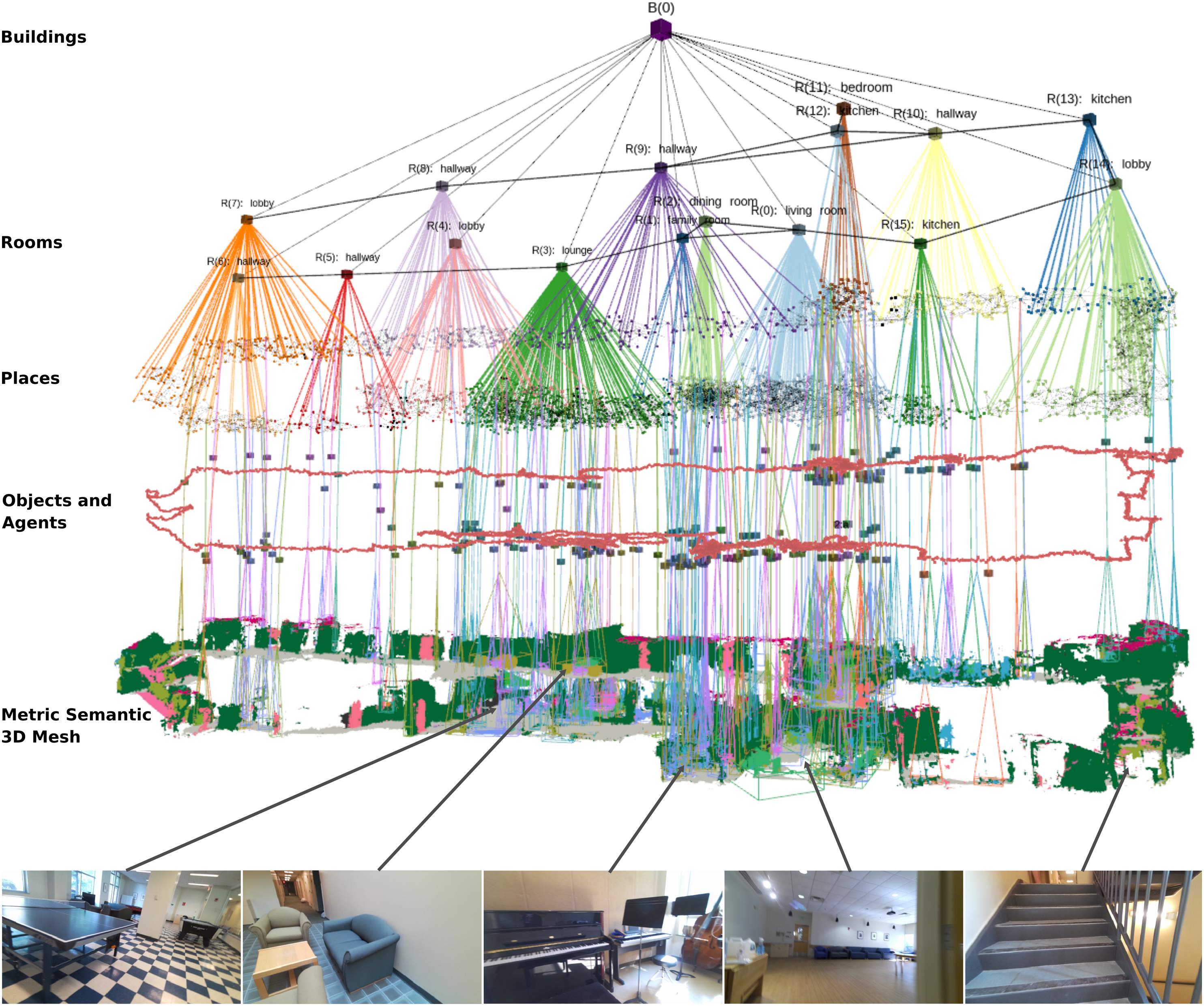

1.2. Real-time systems

While 3D scene graphs can serve as an advanced “mental model” for robots, methods to build such a rich representation in real-time remain largely unexplored. The works (Kim et al., 2019; Wald et al., 2020; Wu et al., 2021) allow real-time operation but are restricted to “flat” 3D scene graphs that only include objects and their relations while disregarding the top layers in Figure 1. The works (Armeni et al., 2019; Rosinol et al. 2020b, 2021), which focus on building truly hierarchical representations, run offline and require several minutes to build a 3D scene graph (Armeni et al. (2019) even assumes the availability of a complete metric-semantic mesh of the environment built beforehand). Extending our prior works (Rosinol et al., 2020b, 2021) to operate in real-time is non-trivial. These works utilize an Euclidean Signed Distance Function (ESDF) of the entire environment to build the scene graph. Unfortunately, ESDFs memory requirements scale poorly in the size of the environment; see Oleynikova et al. (2017) and Section 2. Moreover, the extraction of places and rooms in Rosinol et al. (2021, 2020b) involves batch algorithms that process the entire ESDF, whose computational cost grows over time and is incompatible with real-time operation. Finally, the ESDF is reconstructed from the robot trajectory estimate which keeps changing in response to loop closures. The approaches (Rosinol et al., 2020b, 2021) would therefore need to rebuild the scene graph from scratch after every loop closure, clashing with real-time operation.

The present paper extends our prior work (Hughes et al., 2022) and proposes the first real-time system to build hierarchical 3D scene graphs of large-scale environments. Following (Hughes et al., 2022), recent works has explored constructing situational graphs (Bavle et al. 2022b, 2022a), a hierarchical representation for scene geometry with layers describing free-space traversability, walls, rooms, and floors. While related to this research line, the works (Bavle et al. 2022b, 2022a) focus on LIDAR-based systems, which mostly reason over geometric features (e.g., walls, rooms, floors), but lack the rich semantics we consider in this paper (e.g., objects and room labels). We postpone a more extensive literature review to Section 7.

1.3. Contribution 1: Foundations of hierarchical representations (Section 2)

We start by observing that flat metric-semantic representations scale poorly in the size of the environment and the size of the vocabulary of semantic labels the robot has to incorporate in the map. For instance, a voxel-based metric-semantic map picturing the floor of an office building with 40 semantic labels per voxel (as the one underlying the approaches of Rosinol et al. (2021) and Grinvald et al. (2019)) already requires roughly 450 MiB to be stored. Envisioning future robots to operate on much large scales (e.g., an entire city) and using a much larger vocabulary (e.g., the English dictionary includes roughly 500,000 words), we argue that research should move beyond flat representations. We show that hierarchical representations allow to largely reduce the memory requirements, by enabling lossless compression of semantic information into a layered graph, as well as lossy compression of the geometric information into meshes and graph-structured representations of the free space. Additionally, we show that hierarchical representations are amenable for efficient inference. In particular, we prove that the layered graphs appearing in hierarchical map representations have small treewidth, a property that enables efficient inference; for instance, we conclude that the treewidth of the scene graph modeling an indoor environment does not scale with the number of nodes in the graph (i.e., roughly speaking, the number of nodes is related to the size of the environment), but rather with the maximum number of objects in each room. While most of the results above are general and apply to a broad class of hierarchical representations, we conclude this part by introducing a specific hierarchical representation for indoor environments, namely 3D scene graphs.

1.4. Contribution 2: Real-time incremental 3D scene graph construction (Section 3)

After establishing the importance of hierarchical representations, we move to developing a suite of algorithms to estimate 3D scene graphs from sensor data. In particular, we develop real-time algorithms that can incrementally estimate a 3D scene graph of an unknown building from visual-inertial sensor data. We use existing methods for geometric processing to incrementally build a metric-semantic mesh of the environment and reconstruct a sparse graph of “places”; intuitively, the mesh describes the occupied space (including objects in the environment), while the graph of places provides a succinct description of the free space. Then we propose novel algorithms to efficiently cluster the places into rooms; here, we use tools from topology, and in particular the notion of persistent homology (Huber 2021). Finally, we use novel architectures for geometric deep learning, namely neural trees (Talak et al., 2021), to infer the semantic labels of each room (e.g., bedroom, kitchen, etc.) from the labels of the object within. Towards this goal, we show that our 3D scene graph representation allows to quickly and incrementally compute a tree decomposition of the 3D scene graph, which—together with our bound on the scene graph treewidth—ensures that the neural tree runs in real-time on an embedded GPU.

1.5. Contribution 3: Persistent representations via hierarchical loop closure detection and 3D scene graph optimization (Section 4)

Building a persistent map representation requires the robot to recognize that it is revisiting a location it has seen before, and correcting the map accordingly. We propose a novel hierarchical approach for loop closure detection: the approach involves (i) a top-down loop closure detection that uses hierarchical descriptors—capturing statistics across layers in the scene graph—to find putative loop closures, and (ii) a bottom-up geometric verification that attempts estimating the loop closure pose by registering putative matches. Then, we propose the first algorithm to optimize a 3D scene graph in response to loop closures; our approach relies on embedded deformation graphs (Sumner et al., 2007) to simultaneously and consistently correct all the layers of the scene graph, including the 3D mesh, objects, places, and the robot trajectory.

1.6. Contribution 4: Hydra, a real-time spatial perception system (Section 5)

We conclude the paper by integrating the proposed algorithms into a highly parallelized perception system, named Hydra, that combines fast early and mid-level perception processes (e.g., local mapping) with slower high-level perception (e.g., global optimization of the scene graph). We demonstrate Hydra in challenging simulated and real datasets, across a variety of environments, including an apartment complex, an office building, and two student residences. Our experiments (Section 6) show that (i) we can reconstruct 3D scene graphs of large, real environments in real-time, (ii) our online algorithms achieve an accuracy comparable to batch offline methods and build a richer representation compared to competing approaches (Wu et al., 2021), and (iii) our loop closure detection approach outperforms standard approaches based on bag-of-words and visual-feature matching in terms of quality and quantity of detected loop closures. The source code of Hydra is publicly available at https://github.com/MIT-SPARK/Hydra.

1.7. Novelty with respect to Hughes et al. (2022); Talak et al. (2021)

This paper builds on our previous conference papers (Hughes et al., 2022; Talak et al., 2021) but includes several novel findings. First, rather than postulating a 3D scene graph structure as done in Hughes et al. (2022), we formally show that hierarchical representations are crucial to achieve scalable scene understanding and fast inference. Second, we propose a novel room segmentation method based on the notion of persistent homology, as a replacement for the heuristic method in Hughes et al. (2022). Third, we develop novel learning-based hierarchical descriptors for place recognition, that further improve performance with respect to the handcrafted hierarchical descriptors in Hughes et al. (2022). Fourth, the real-time system described in this paper is able to also assign room labels, leveraging the neural tree architecture from Talak et al. (2021); while Talak et al. (2021) uses the neural tree over small graphs corresponding to a single room, in this paper we provide an efficient way to obtain a tree decomposition of the top layers of the scene graph, hence extending Talak et al. (2021) to simultaneously operate over all rooms and account for their relations. Finally, this paper includes further experiments and evaluations on real robots (Clearpath Jackal robots and Unitree A1 robots) and comparisons with recent scene graph construction baselines (Wu et al., 2021).

2. Symbol grounding and the need for hierarchical representations

The goal of this section is twofold. First, we remark that in order to support the execution of complex instructions, map representations must be metric-semantic, and hence ground symbolic knowledge (i.e., semantic aspects in the scene) into the map geometry (Section 2.1). Second, we observe that “flat” representations, which naively store semantic attributes for each geometric entity in the map (e.g., attach semantic labels to each voxel in an ESDF) scale poorly in the size of the environment; on the other hand, hierarchical representations scale better to large environments (Section 2.2) and enable efficient inference (Section 2.3). We conclude the section by introducing the notion of a 3D scene graph, an example of a hierarchical representation for indoor environments, and discussing its structure and properties (Section 2.4).

2.1. Symbols and symbol grounding

High-level instructions issued by humans (e.g., “go and pick up the chair”) involve symbols. A symbol is the representation of a concept that has a specific meaning for a human (e.g., the word “chair” is a symbol in the sense that, as humans, we understand the nature of a chair). For a symbol to be useful to guide robot action, it has to be grounded into the physical world. For instance, for the robot to correctly execute the instruction “go and pick up the chair,” the robot needs to ground the symbol “chair” to the physical location the chair is situated in. ¹ In principle, we could design the perception system of our robot to ground symbols directly in the sensor data. For instance, a robot with a camera could map image pixels to appropriate symbols (e.g., “chair,” “furniture,” “kitchen,” “apartment”), as commonly done in 2D semantic segmentation (Garcia-Garcia et al., 2017). However, grounding symbols directly into sensor data is not scalable: sensor data (e.g., images) is collected at high rates and is relatively expensive to store. This is neither convenient nor efficient when grounding symbols for long-term operation. Instead, we need intermediate (or sub-symbolic) representations that compress the raw sensor data into a more compact format, and that can be used to ground symbols. Traditional geometric map models used in robotics (e.g., 2D occupancy grids or 3D voxel-based maps) can be understood as sub-symbolic representations: each cell in a voxel grid does not represent a semantic concept, and instead is used to ground two symbols: “obstacle” and “free-space.” Therefore, this paper is concerned with building metric-semantic representations, which ground symbolic knowledge into geometric (i.e., sub-symbolic) representations.

2.1.1. Which symbols should a map contain?

In this paper, we directly specify the set of symbols the robot is interested in (i.e., certain classes of objects and rooms, to support navigation in indoor environments). However, it is worth discussing how to choose the symbols more generally. The choice of symbols clearly depends on the task the robot has to execute. A mobile robot may implement a path planning query by just using the “free-space” symbol and the corresponding grounding, while a more complex domestic robot may instead need additional symbols (e.g., “cup of coffee,” “table,” and “kitchen”) and their groundings to execute instructions such as “bring me the cup of coffee on the table in the kitchen.” A potential way to choose the symbols to include in the map therefore consists of inspecting the set of instructions the robot has to execute, and then extracting the list of symbols (e.g., objects and relations of interest) these instructions involve. For instance, in this paper, we mostly focus on indoor environments and assume the robot is tasked with navigating to certain objects and rooms in a building. Therefore, the symbols we include in our maps include free-space, objects, rooms, and buildings. After establishing the list of relevant symbols, the goal is for the robot to build a compact sub-symbolic representation (i.e., a geometric map), and then ground these symbols into the sub-symbolic representation. A pictorial representation of this idea is given in Figure 2(a): the robot builds an occupancy map (sub-symbolic representation) and attaches a number of semantic labels (symbols) to each cell. We refer to this representation as “flat” since each cell is assigned a list of symbols of interest. As we will see shortly, there are more clever ways to store the same information.

Figure 2.

(a) Example of a flat metric-semantic representation. We show labels only for a subset of the cells in the grid map for the sake of readability. (b) Example of hierarchical metric-semantic representation with a grid-map as sub-symbolic layer. (c) A hierarchical metric-semantic representation with compressed sub-symbolic layer. The cells representing each object are compressed into bounding polygons, and the free-space cells are compressed into a sparse graph where each node and edge are also assigned a radius that defines a circle of free-space around it.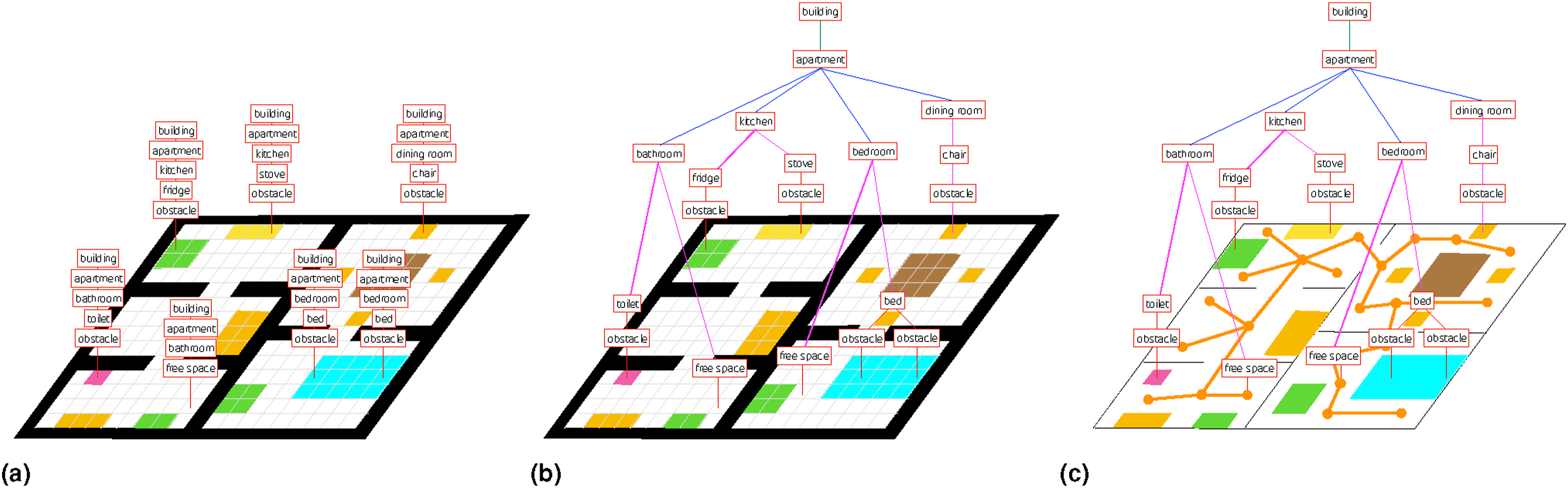

2.2. Hierarchical representations enable large-scale mapping

While the flat representation of Figure 2(a) may contain all the information the robot needs to complete its task, it is unnecessarily expensive to store. Here we show that the symbolic knowledge underlying such representation naturally lends itself to be efficiently stored using a hierarchical representation.

Consider the case where we use a flat representation (as shown in Figure 2(a)) to represent a 3D scene and assume our dictionary contains L symbols of interest. Let δ be the cell (or voxel) size and call V the volume of the scene the representation describes. Then, the corresponding metric-semantic representation would require a memory of:

$m=\mathcal{O}\left(L\cdot V/{\delta }^3\right)$

(1)

to store L labels for each voxel. Note that m grows with the number of symbols L, multiplied by the size of the sub-symbolic representation V/δ³ (i.e., the number of voxels in the volume). When mapping large environments the term V/δ³ quickly becomes unsustainably large; for instance, covering a 10 km × 10 km area with a 10 cm grid resolution, even disregarding the vertical dimension, would require 10¹⁰ voxels. In addition, it would be desirable for the next generation of robots to execute a large set of tasks, hence requiring them to ground a large dictionary of symbols L. ² The size of the sub-symbolic representation, the number of symbols, and their multiplicative relation in (1) make a flat metric-semantic representation unsuitable for large-scale spatial perception.

A key observation here is that multiple voxels encode the same grounded symbols (e.g., a chair). In addition, many symbols naturally admit a hierarchical organization where higher-level concepts (i.e., buildings or rooms for indoor environments) contain lower-level symbols (e.g., objects). This suggests that we can more efficiently store information hierarchically, where all voxels associated with a certain object (e.g., all voxels belonging to a chair) are mapped to the same symbolic node (e.g., an object node with the semantic label “chair”), object nodes are associated with the room they belong to, room nodes are associated to the apartment unit they belong to, and so on. This transforms the flat representation of Figure 2(a) into the hierarchical model of Figure 2(b), where only the lowest level symbols are directly grounded into voxels, while the top layers are arranged hierarchically. This hierarchical representation is more parsimonious and reduces the required memory to

$m=\mathcal{O}\left(V/{\delta }^3+N_{\text{objects}}+N_{\text{rooms}}+\cdots +N_{\text{buildings}}\right),$

(2)

where N_layer (with layer ∈ {objects, rooms, …}) is the number of symbols at the specific layer of the hierarchy. This representation is more memory efficient than (1) because it decouples the number of symbols from the size V/δ³ of the sub-symbolic representation. For instance, the scene in Figure 2 has 336 voxels, and we assume L = 5. ³ Then, the flat representation of Figure 2(a) involves storing 1680 symbols, while Figure 2(b) only requires storing 355 symbols and 354 edges describing their hierarchical relations. Crucially, the compression we performed when moving from Figure 2(a) and (b) is lossless: the two representations contain exactly the same amount of information.

While we “compressed” the symbolic representation using a hierarchical data structure, the term V/δ³ in (2) that corresponds to the sub-symbolic layer is still impractically large for many applications. Therefore, our robots will also typically need some compression mechanism for the sub-symbolic layer that provides a more succinct description of the occupied and free space as compared to voxel-based maps. Fortunately, the mapping literature already offers alternatives to standard 3D voxel-based maps such as OctTree (Zeng et al., 2013) or neural implicit representations (Park et al., 2019). In general, this compression reduces the memory requirement to

$m=\mathcal{O}\left(N_{\text{sub}-\text{sym}}+N_{\text{objects}}+N_{\text{rooms}}+\cdots +N_{\text{buildings}}\right),$

(3)

where N_sub-sym is the size of the compressed sub-symbolic representation. The behavior of N_sub-sym is driven by the compression approach used, but in general N_sub-sym ends up being much smaller than V/δ³; in the ideal case N_sub-sym would grow gracefully with respect to the complexity of the scene and the resolution required by the task. We show a notional example of a compressed sub-symbolic layer in Figure 2(c). This can represent the 336 original cells of the sub-symbolic layer of Figure 2(b) with roughly 23 nodes, 22 edges, and a 2D polygonal mesh with roughly 132 vertices. Note that moving from Figure 2(b) and (c) may entail a lossy compression of the sub-symbolic layer, i.e., the compressed representation may only be an approximate representation of the geometry of the environment. The general idea is that we can always compress the sub-symbolic representation to fit into the available memory of our robot, although such a compression might induce some performance degradation in the execution of the task (e.g., coarser maps might lead to longer paths in motion planning).

2.3. Hierarchical representations enable efficient inference

While above we showed that hierarchical representations are more scalable in terms of memory requirements, this section shows that the graphs underlying hierarchical representations also enable fast inference. Specifically, we show that these hierarchical graphs have small treewidth: their treewidth does not grow with the size of the graph (i.e., proportionally to the size of the explored scene), but rather with the treewidth of each layer in the hierarchy. The treewidth is a well-known measure of complexity for many problems on graphs (Bodlaender 2006; Dechter and Mateescu 2007; Feder and Vardi 1993; Grohe et al., 2020). Chandrasekaran et al. (2008) show that the graph treewidth is the only structural parameter that influences tractability of probabilistic inference on graphical models: while inference is NP-hard in general for inference on graphical models (Cooper 1990), proving that a graph has small treewidth opens the door to efficient, polynomial-time inference algorithms. Additionally, in our previous work we have shown that the treewidth is also the main factor impacting the expressive power and tractability of novel graph neural tree architectures, namely neural trees (Talak et al., 2021). The results in this section therefore open the door to the efficient use of powerful tools for learning over graphs; see Section 3.4.2.

In the rest of this section, we formalize the notion of hierarchical graph and show that the treewidth of a hierarchical graph is always bounded by the maximum treewidth of each of its layers. We do this by proving that the tree decomposition of the hierarchical graph can be obtained by a suitable concatenation of the tree decompositions of its layers. The results in this section are general and apply to arbitrary hierarchical representations (as defined below) beyond the representations of indoor environments we consider later in the paper.

Definition 1

Hierarchical Graph. A graph $\mathcal{G}=\left(\mathcal{V},\mathcal{E}\right)$ is said to be a hierarchical graph if the set of nodes $\mathcal{V}$ can be partitioned into ℓ layers, i.e., $\mathcal{V}={\cup }_{i=1}^{\ell }{\mathcal{V}}_i$ , such that

1. Single parent: each node $v\in {\mathcal{V}}_i$ at layer i shares an edge with at most one node in the layer ${\mathcal{V}}_{i+1}$ above,

2. Locality: each $v\in {\mathcal{V}}_i$ can only share edges with nodes in the same or adjacent layers, i.e., ${\mathcal{V}}_{i-1}$ , ${\mathcal{V}}_i$ , or ${\mathcal{V}}_{i+1}$ ,

3. Disjoint children: for any $u,v\in {\mathcal{V}}_i$ the children of u and v, namely C(v) and C(u) are disjoint (i.e., they share no nodes or edges), where

$C\left(u\right)\triangleq \left\{w\in {\mathcal{V}}_{i-1} | \left(w,u\right)\in \mathcal{E}\right\}$

(4)

denotes the children of u, i.e., the set of nodes in layer ${\mathcal{V}}_{i-1}$ sharing an edge with u.

We refer to $\mathcal{G}$ as an ℓ-layered hierarchical graph and denote with ${\mathcal{V}}_i$ the set of nodes in layer i. Moreover, we conventionally order the layers from the bottom to the top, i.e., the lowest layer is ${\mathcal{V}}_1$ , while the top layer is ${\mathcal{V}}_{\mathcal{l}}$ .

To gain some insight into Definition 1, consider a hierarchical graph where the bottom layer ${\mathcal{V}}_1$ describes the objects in the environment, while the higher layers ${\mathcal{V}}_2$ and ${\mathcal{V}}_3$ describe room and buildings, respectively. Then, the first condition in Definition 1 requires that each object belongs to a single room, and each room belongs to a single building. The second condition restricts the inter-layer edges to connect objects to rooms, and rooms to buildings. Finally, the third condition says that objects in a room are not connected to objects in another room, and that rooms in a building do not share edges with rooms in other buildings. These conditions are relatively mild; they are easily met when edges in the graph represent inclusion or adjacency (i.e., for the graphs considered in the rest of this paper).

We now show that a tree decomposition of a hierarchical graph can be constructed by concatenating the tree decomposition of each of its layers. This result will allow us to obtain the treewidth bound in Proposition 3. The resulting tree decomposition algorithm (Algorithm 1) will also be used in the neural tree approach used for room classification in Section 3.4.2. The interested reader can find a refresher about tree decomposition and treewidth in Appendix A.1 ⁴ and an example of execution of Algorithm 1 in Figure 3. In the following we assume that the provided hierarchical graph is undirected, or is obtained from a directed graph through moralization (Koller and Friedman 2009).

Figure 3.

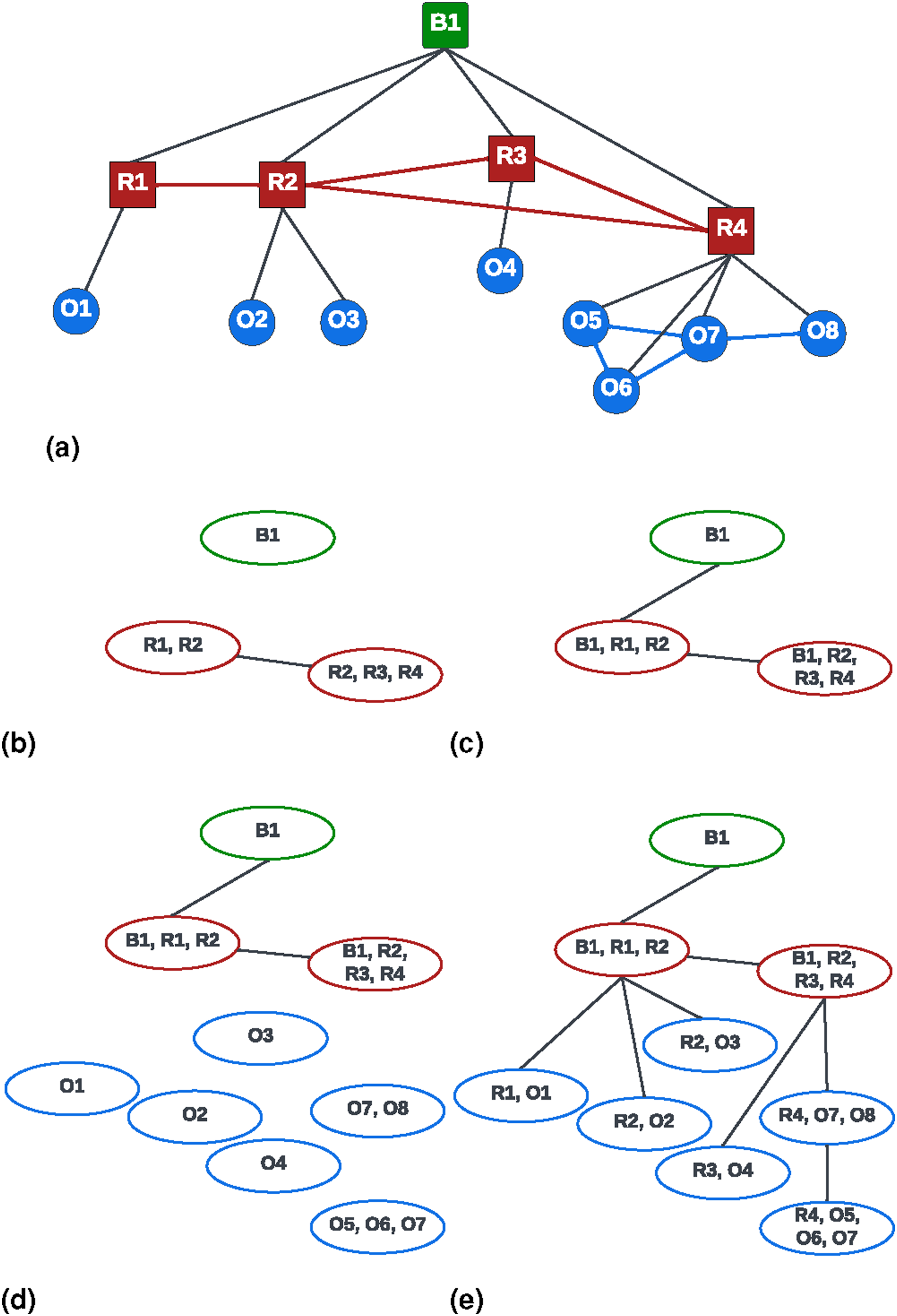
(a) Hierarchical object-room-building graph with objects O1, O2, … O8, rooms R1, R2, R3, R4, and a single building B1. (b) Tree decomposition T of the building B1 and associated T _v of the rooms (i.e., children of B1) as computed in line 2 and 8 of Algorithm 1. (c) T after adding B1 to every bag of the tree decomposition of the rooms and joining T _v to T (line 8 and line 8 in Algorithm 1). (d) T and associated T _v for the object nodes. (e) Final tree decomposition of the object-room-building graph formed by the concatenation procedure described in Algorithm 1.

Theorem 2

Tree Decomposition of Hierarchical Graph. Let $\mathcal{G}=\left(\mathcal{V}={\cup }_{i=1}^{\ell }{\mathcal{V}}_i,\mathcal{E}\right)$ be an ℓ-layered undirected hierarchical graph. Let T be the tree decomposition of the sub-graph spanned by ${\mathcal{V}}_{\ell }$ (top layer) and T _v be the tree decomposition of the sub-graph spanned by the children C _i (v) of v, for $v\in {\mathcal{V}}_i$ and i = ℓ, …, 2. Then a tree decomposition for graph $\mathcal{G}$ can be constructed from $\{T_v | v\in {\mathcal{V}}_i$ and $i=\ell ,\mathcal{\dots },2\}$ and T, by the simple concatenation procedure described in Algorithm 1.

Proof

(i) Notation: Given a subset of nodes $\overline{\mathcal{V}}\subseteq \mathcal{V}$ of the graph $\mathcal{G}\left(\mathcal{V},\mathcal{E}\right)$ , we denote with $\mathcal{G}\left[\overline{\mathcal{V}}\right]$ the sub-graph of $\mathcal{G}$ containing nodes $\overline{\mathcal{V}}$ and including all edges in $\mathcal{E}$ having both endpoints in $\overline{\mathcal{V}}$ . We then denote the tree decomposition of a graph $\mathcal{G}$ by $T=\left(B,E\right)=\text{TD}\left[\mathcal{G}\right]$ , where B denotes the collection of bags and E denotes the set of edges in the tree decomposition graph T. For a tree decomposition graph T = (B, E) and any node w (not already included in any of the bags b ∈ B), we denote T + {w} to be the tree decomposition T, after adding the element w to every bag in T. Finally, given two disjoint trees T, T′ and an edge (b, b′) with b ∈ T and b′ ∈ T′, we use T ← T ⊕ T′ ⊕ (b, b′) to indicate updating graph T by adding graph T′, along with the edge (b, b′) to it.

(ii) Intuitive Explanation of Algorithm 1: We form the tree decomposition T of the hierarchical graph sequentially. We initialize T with the tree decomposition of the top layer graph ${\mathcal{G}}_{\mathcal{l}}=\mathcal{G}\left[{\mathcal{V}}_{\mathcal{l}}\right]$ . We then augment T with the tree decomposition graphs T _v of C(v), for each $v\in {\mathcal{V}}_{\mathcal{l}}$ . We augment bags of T _v with element {v} to mark the fact that v connects each node in C(v) (in graph $\mathcal{G}$ ). This procedure is carried out for the remaining layers i = ℓ − 1, …, 2 and all nodes $v\in {\mathcal{V}}_i$ .

Figure 3 shows an example of execution of Algorithm 1 for the graph in Figure 3(a). Figure 3(b) shows the (disconnected) tree decompositions produced by line 2 (which produces the single green bag B1) and the first execution of line 8 (i.e., for i = ℓ, which produces the two red bags). Figure 3(c) shows the result produced by the first execution of line 8 and line 8, which adds B1 to all the red bags, and then connects the two tree decompositions with an edge, respectively. Figure 3(d) and (e) shows the result produced by the next iteration of the algorithm.

(iii) Proof: Recall that a tree decomposition T = (B, E) of a graph $\mathcal{G}=\left(\mathcal{V},\mathcal{E}\right)$ must satisfy the following conditions:

C1 T must be a tree;

C2 Every bag b ∈ B must be a subset of nodes of the given graph $\mathcal{G}$ , i.e., $b\subseteq \mathcal{V}$ ;

C3 For all edges $\left(u,v\right)\in \mathcal{E}$ in the given graph $\mathcal{G}$ , there must exist a bag b ∈ B such that u, v ∈ b;

C4 For every node $v\in \mathcal{V}$ in the given graph $\mathcal{G}$ , the set of bags {b ∈ B | v ∈ b} must form a connected component in T;

C5 For every node 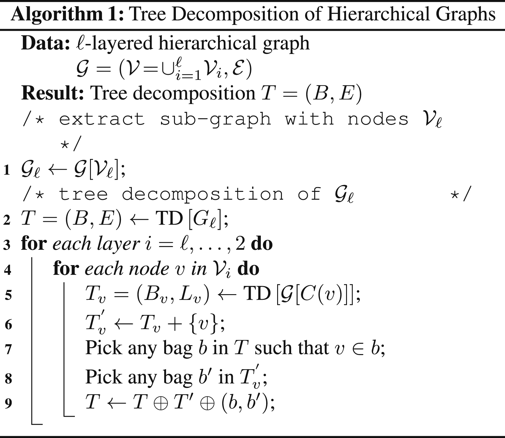$v\in \mathcal{V}$ in the given graph $\mathcal{G}$ , there must exist a bag b ∈ B that contains it, i.e., v ∈ b. To state this in another way: ${\cup }_{b\in B}\left\{v\in b\right\}=\mathcal{V}$ .

Algorithm 1 constructs a tree decomposition T of $\mathcal{G}$ sequentially by exploring the graph, by layers (going from layer-ℓ to layer 1) and by nodes v in each layer. Let ${\mathcal{G}}_t^e$ denote the sub-graph of $\mathcal{G}$ that is explored by Algorithm 1, until iteration t. Here, we count an iteration to be the execution of Line 9, and count the initialization at Line 2 as the first iteration (i.e., the first iteration initializes the tree decomposition, while the subsequent iterations update the tree decomposition).

We prove that, at any iteration t, the tree decomposition graph T constructed in Algorithm 1 is a valid tree decomposition of the graph ${\mathcal{G}}_t^e$ . We prove this by induction. At t = 1, the explored graph ${\mathcal{G}}_1^e$ is nothing but ${\mathcal{G}}_{\mathcal{l}}$ . Note that T, after iteration 1 (i.e., after the initialization at Line 2) by definition equals the tree decomposition ${\mathcal{G}}_1^e$ . Now we only need to prove that subsequent iterations produce a tree decomposition of ${\mathcal{G}}_t^e$ . Each new iteration (i.e., execution of Line 9) updates T to include $T_v^{\prime }$ and the edge (b, b′). The new explored graph is ${\mathcal{G}}_{t+1}^e={\mathcal{G}}_t^e\oplus \mathcal{G}\left[C\left(v\right)+\left\{v\right\}\right]$ . It suffices to argue that $T\oplus T_v^{\prime }\oplus \left(b,b^{\prime }\right)$ (Lines 5 to 9) is a valid tree decomposition of ${\mathcal{G}}_{t+1}^e={\mathcal{G}}_t^e\oplus \mathcal{G}\left[C\left(v\right)+\left\{v\right\}\right]$ . We argue this by proving that the requirements C1–C5 are satisfied.

For C1, we note that $T\oplus T_v^{\prime }\oplus \left(b,b^{\prime }\right)$ is a tree as T and $T_v^{\prime }$ are disjoint trees and (b, b′) is an edge connecting the two trees, T and $T_v^{\prime }$ . C2 is satisfied because T and $T_v^{\prime }$ are tree decompositions of sub-graphs of $\mathcal{G}$ . C3 is satisfied for all edges in ${\mathcal{G}}_t^e$ and in $\mathcal{G}\left[C\left(v\right)\right]$ . The only edges that remain are those that connect node v to nodes in C(v), namely {(v, u) | u ∈ C(v)}. We note that by adding {v} to every bag of T _v to obtain $T_v^{\prime }$ we get that all such edges are also included in the bags of $T_v^{\prime }$ . C4 is satisfied again because T and T _v are valid tree decompositions and $T_v^{\prime }$ is built from T _v by adding v to all bags of T _v . As T _v is a tree graph disjoint from T, we retain property C4. ${\mathcal{G}}_{t+1}^e={\mathcal{G}}_t^e\oplus \mathcal{G}\left[C\left(v\right)+\left\{v\right\}\right]$ (i.e., nodes in ${\mathcal{G}}_t^e$ and C(v)), have a bag in $T\oplus T_v^{\prime }\oplus \left(b,b^{\prime }\right)$ .

Theorem 2 above showed that we can easily build a tree decomposition of a hierarchical graph by cleverly “gluing together” tree decompositions of sub-graphs in the hierarchy. Now we want to use that result to bound the treewidth of a hierarchical graph $\mathcal{G}$ . Each node in the tree decomposition is typically referred to as a bag, and intuitively represents a subset of nodes in the original graph. The treewidth of a tree decomposition T is defined as the size of the largest bag minus one (see Appendix A.1). The treewidth of a graph $\mathcal{G}$ is then defined as the minimum treewidth that can be achieved among all tree decompositions of $\mathcal{G}$ . Since Algorithm 1 describes one such tree decompositions, Theorem 2 implies the following upper bound on the treewidth of a hierarchical graph.

Proposition 3

Treewidth of Hierarchical Graph. The treewidth $\text{tw}\left[\mathcal{G}\right]$ of an ℓ-layered undirected hierarchical graph $\mathcal{G}$ is bounded by the treewidths of the sub-graphs $\mathcal{G}\left[C\left(v\right)\right]$ spanned by the children C(v) of every node v in $\mathcal{G}$ and the treewidth of the graph $\mathcal{G}\left[{\mathcal{V}}_{\ell }\right]$ spanned by all layer-ℓ nodes:

$tw\left[\mathcal{G}\right]\le \max \left\{\underset{v\in \mathcal{V}}{\max }\left\{tw\left[\mathcal{G}\left[C\left(v\right)\right]\right]+1\right\},tw\left[\mathcal{G}\left[{\mathcal{V}}_{\ell }\right]\right]\right\}.$

(5)

Intuitively, the proposition states that the treewidth of a hierarchical graph does not grow with the number of nodes in the graph, but rather with the treewidth (roughly speaking, the complexity) of each layer in the graph.

2.4. 3D scene graphs and indoor environments

While the considerations in the previous sections apply to generic hierarchical representations, in this section we tailor the discussion to a specific hierarchical representation, namely a 3D scene graph, and discuss its structure and properties when such representation is used to model indoor environments.

2.4.1. Choice of symbols for indoor navigation

We focus on indoor environments and assume the robot is tasked with navigating to certain objects and rooms in a building. Therefore, we include the following groups of symbols that form the layers in our hierarchical representation: free-space, obstacles, objects and agents, rooms, and building. The details of the label spaces that we use for the object and room symbols can be found in Appendix A.4. The only “agent” in our setup is the robot mapping the environment. In terms of relations between symbols, we mostly consider two types of relations: inclusion (i.e., the chair is in the kitchen) and adjacency or traversability (i.e., the chair is near the table, the kitchen is adjacent to/reachable from the dining room).

As we mentioned in Section 2.2, this choice of symbols and relations is dictated by the tasks we envision the robot to perform and therefore it is not universal. For instance, other tasks might require breaking down the free-space symbol into multiple symbols (e.g., to distinguish the front from the back of a room), or might require considering other agents (e.g., humans moving in the environment as in Rosinol et al. (2021; 2020b)). This dependence on the task also justifies the different definitions of a 3D scene graph found in recent literature: for instance, the original proposal in Armeni et al. (2019) focuses on visualization and human-machine interaction tasks, rather than robot navigation, hence the corresponding scene graphs do not include the free-space as a symbol; the proposals Wu et al. (2021); Kim et al. (2019) consider smaller-scale tasks and disregard room and building symbols. Similarly, the choice of relations is task dependent and can include a much broader set of relations beyond inclusion and adjacency. For instance, relations can describe attributes of an object (e.g., “has color”), material properties (e.g., “is made of”), can be used to compare entities (e.g., “is taller than”), or may encode actions (e.g., a person “carries” an object, a car “drives on” the road). While these other relations are beyond the scope of our paper, we refer the reader to Zhu et al. (2022) for further discussion.

2.4.2. Choice of sub-symbolic representations

We ground each symbol in compact sub-symbolic representations; intuitively, this reduces to attaching geometric attributes to each symbol observed by the robot. We ground the “obstacle” symbol into a 3D mesh describing the observed surfaces in the environment. We ground the “free-space” symbol using a places sub-graph, which can be understood as a topological map of the environment. Specifically, each place node in the graph of places is associated with an obstacle-free 3D location (more precisely, a sphere of free space described by a centroid and radius), while edges represent traversability between places. ⁵ We ground the “agent” symbol using the pose graph describing the robot trajectory (Cadena et al., 2016). We ground each “object,” “room,” and “building” symbol using a centroid and a bounding box. Somewhat redundantly, we also store the mesh vertices corresponding to each object, and the set of places included in each room, which can be also understood as additional groundings for these symbols. As discussed in the next section, this is mostly a byproduct of our algorithms, rather than a deliberate choice of sub-symbolic representation.

2.4.3. 3D scene graphs for indoor environments

The choices of symbolic and sub-symbolic representations outlined above lead to the 3D scene graph structure visualized in Figure 1. In particular, Layer 1 is a metric-semantic 3D mesh. Layer 2 is a sub-graph of objects and agents; each object has a semantic label (which identifies the symbol being grounded), a centroid, and a bounding box (providing the grounding); each agent is modeled by a pose graph describing its trajectory (in our case the robot itself is the only agent). Layer 3 is a sub-graph of places (i.e., a topological map) where each place is an obstacle-free location and an edge between places denotes straight-line traversability. Layer 4 is a sub-graph of rooms where each room has a centroid, and edges connect adjacent rooms. Layer 5 is a building node connected to all rooms (we assume the robot maps a single building). Edges connect nodes within each layer (e.g., to model traversability between places or rooms, or connecting nearby objects) or across layers (e.g., to model that mesh vertices belong to an object, that an object is in a certain room, or that a room belongs to a building). Note that the object-room-building subgraph of the proposed 3D scene graph structure is a hierarchical graph fulfilling the conditions of Definition 1.

Our 3D scene graph definition has been shown to be a suitable model to support various indoor tasks in robotics. Ravichandran et al. (2022) show that the use of 3D scene graphs improves peformance in RL-based object search. Other works have examined the benefits of hierarchical representations for planning efficiency, including path-planning (Rosinol et al., 2021) and symbolic task planning (Agia et al., 2022). More recently, Rana et al. (2023) use 3D scene graphs for indoor mobile manipulation tasks, using the hierarchy present in the representation to ground tasks specified in natural language. While these examples of early adoption of our 3D scene graph definition provide reassuring evidence of the “actionable” nature of our representation, we remind the reader that our definition is not intedend to be universal to all indoor robotics tasks. Instead, we intend this definition to be a foundation that can be easily extended in a task-driven manner.

2.4.4. Treewidth of indoor 3D scene graphs

In Section 2.3 we concluded that the treewidth of a hierarchical graph is bounded by the treewidth of its layers. In this section, we particularize the treewidth bound to 3D scene graphs modeling indoor environments. We first prove bounds on the treewidth of key layers in the 3D scene graph (Lemmas 4 and 5). Then we translate these bounds into a bound on the treewidth of the object-room-building sub-graph of a 3D scene graph (Proposition 6); the bound is important in practice since we will need to perform inference over such a sub-graph to infer the room (and potentially building) labels, see Section 3.4.2.

We start by bounding the treewidth of the room layer.

Lemma 4

Treewidth of Room Layer. Consider the sub-graph of rooms, including the nodes in the room layer of a 3D scene graph and the corresponding edges. If each room connects to at most two other rooms that have doors (or more generally passage ways) leading to other rooms, then the room graph has treewidth bounded by two.

The insight behind Lemma 4 is that the room sub-graph is not very far from a tree (i.e., it has low treewidth) as long as there are not many rooms with multiple doors (or passage ways). In particular, the room sub-graph has treewidth equal to 2 if each room has at most two passage ways to other rooms with multiple entries. Note that the theorem statement allows a room to be connected to an arbitrary number of rooms with a single entry (i.e., a corridor leading to multiple rooms that are only accessible via that corridor). Figure 4(a) reports empirical upper-bounds of the treewidth of the room sub-graphs in the 90 scenes of the Matterport3D dataset (Chang et al., 2017) (see Section 6 for more details about the experimental setup). The observed treewidth is at most 2, confirming that the conclusions of Lemma 4 hold in several apartment-like environments.

Figure 4.

Histogram of the treewidth upper-bounds for (a) the room sub-graph and (b) the object sub-graph of the 3D scene graphs obtained using the 90 scenes of the Matterport3D dataset Chang et al. (2017). We use the minimum-degree and the minimum-fill-in heuristic to obtain treewidth upper-bounds (Bodlaender and Koster 2010). We then compute an upper-bound to be the lowest of the two.

Lemma 5

Treewidth of Object Layer. Consider the sub-graph of objects, which includes the nodes in the object layer of a 3D scene graph and the corresponding edges. The treewidth of the object sub-graph is bounded by the maximum number of objects in a room.

The result is a simple consequence of the fact that in our 3D scene graph, there is no edge connecting objects in different rooms, therefore, the graph of objects includes disconnected components corresponding to each room, whose treewidth is bounded by the size of that connected component, i.e., the number of objects in that room. Figure 4(b) reports the treewidth upper-bounds for the object sub-graphs in the Matterport3D dataset. We observe that the treewidth of the object sub-graphs tends to be larger compared to the room sub-graphs, but still remains relatively small (below 20) in all tests.

We can now conclude with a bound on the treewidth of the object-room-building graph in a 3D scene graph.

Proposition 6

Treewidth of the Object-Room-Building Graph. Consider the object-room-building graph of a building, including the nodes in the object, room, and building layers of a 3D scene graph and the corresponding edges. Assume the treewidth of the room graph is less than the treewidth of the object graph. Then, the treewidth $\text{tw}\left[\mathcal{G}\right]$ of the object-room-building graph $\mathcal{G}$ is bounded by

$tw\left[\mathcal{G}\right]\le 1+N_o,$

(6)

where N_o denotes the largest number of objects in a room.

Proposition 6 indicates that the treewidth of the object-room-building graph does not grow with the size of the scene graph, but rather depends on how cluttered each room is. This is in stark contrast with the treewidth of social network graphs (Maniu et al., 2019; Talak et al., 2021), and further motivates the proposed hierarchical organization. The treewidth bounds in this section open the door to tractable inference techniques; in particular, in Section 3.4.2, we show they allow applying novel graph-learning techniques, namely, the neural tree (Talak et al., 2021).

Remark 7

Directed vs. Undirected Graphs. We note that the treewidth bounds in Proposition 3, Lemma 4, Lemma 5, and Proposition 6 assume that the given hierarchical graph is undirected, as treewidth is only defined for undirected graphs. When performing inference on directed graphs, a common technique is to convert the directed graph to an undirected graph through the process of moralization (Koller and Friedman 2009). We note that the treewidth bound of Lemma 5 for is a worst-case bound that assumes that the objects in each room form a complete graph. As such, this bound also holds for any undirected graph resulting from moralization of a directed object sub-graph.

3. Real-time incremental 3D scene graph layers construction

This section describes how to estimate an odometric 3D scene graph directly from visual-inertial data as the robot explores an unknown environment. Section 4 then shows how to correct the scene graph in response to loop closures.

We start by reconstructing a metric-semantic 3D mesh to populate Layer 1 of the 3D scene graph (Section 3.1), and use the mesh to extract the objects in Layer 2 (Section 3.2). We extract the places in Layer 3 as a byproduct of the 3D mesh computation by first computing a Generalized Voronoi Diagram (GVD) of the environment, and then approximating the GVD as a sparse graph of places (Section 3.3). We then populate the rooms in Layer 4 by segmenting their geometry using persistent homology (Section 3.4.1) and assigning them a semantic label using the neural tree (Section 3.4.2). In this paper, we assume that the scene we reconstruct consists of a single building, and for Layer 5 we instantiate a single building node that we connect to all estimated room nodes.

3.1. Layers 1: Mesh

We build a metric-semantic 3D mesh (Layer 1 of the 3D scene graph) using Kimera (Rosinol et al., 2020a) and Voxblox (Oleynikova et al., 2017). In particular, we maintain a metric-semantic voxel-based map within an active window around the robot. Each voxel of the map contains free-space information and a distribution over possible semantic labels. We gradually convert this voxel-based map into a 3D mesh using marching cubes, attaching a semantic label to each mesh vertex. This is now standard practice (e.g., the same idea was used in Whelan et al. (2012) without inferring the semantic labels) and the expert reader can safely skip the rest of this subsection.

In more detail, for each keyframe, ⁶ we use a 2D semantic segmentation network to obtain a pixel-wise semantic segmentation of the RGB image, and reconstruct a depth-map using stereo matching (when using a stereo camera) or from the depth channel of the sensor (when using an RGB-D camera). We then convert the semantic segmentation and depth into a semantically-labeled 3D point cloud and transform it according to the odometric estimate of the robot pose (Section 3.2). We use Voxblox (Oleynikova et al., 2017) to integrate the semantically-labeled point cloud into a Truncated Signed Distance Field (TSDF) using ray-casting, and Kimera (Rosinol et al., 2021) to perform Bayesian updates over the semantic label of each voxel during ray-casting. Both Voxblox (Oleynikova et al., 2017) and Kimera (Rosinol et al., 2021) operate over an active window, i.e., only reconstruct a voxel-based map within a user-specified radius r _a around the robot (r _a = 8 m in our tests) ⁷ to bound the memory requirements. Within the active window, we extract the 3D metric-semantic mesh using Voxblox’ marching cubes implementation, where each mesh vertex is assigned the most likely semantic label from the corresponding voxel. We then use spatial hashing (Nießner et al., 2013) to integrate ${\mathcal{M}}_a$ , the mesh inside the active window, into the full mesh ${\mathcal{M}}_f$ , optionally also compressing the mesh to a given resolution. The use of the active window circumvents the need to maintain a monolithic and memory-hungry voxel-based representation of the entire environment (as done in our original proposal in Rosinol et al. (2020a)), and instead allows to gradually transform the voxel-based map in the active window (moving with the robot) into a lighter-weight 3D mesh. The full mesh, ${\mathcal{M}}_f$ , is uncorrected for odometric drift, and we address loop closure detection and optimization in Section 4.

3.2. Layers 2: Objects and agents

3.2.1. Agents

The agent layer consists of the pose graph describing the robot trajectory (we refer the reader to Rosinol et al. (2021) for extensions to multiple agents, including humans). During exploration, the odometric pose graph is obtained using stereo or RGB-D visual-inertial odometry, which is also available in Kimera (Rosinol et al., 2020a, 2021). The poses in the pose graph correspond to the keyframes selected by Kimera, and for each pose we also store visual features and descriptors, which are used for loop closure detection in Section 4. As usual, edges in the pose graph correspond to odometry measurements between consecutive poses, while we will also add loop closures as described in Section 4.

3.2.2. Objects

The object layer consists of a graph where each node corresponds to an object (with a semantic label, a centroid, and a bounding box) and edges connect nearby objects. After extracting the 3D mesh within the active window, we segment objects by performing Euclidean clustering (Rusu 2009) on ${\mathcal{V}}_a$ , the vertices of ${\mathcal{M}}_a$ . In particular, we independently cluster the sets of vertices ${\mathcal{V}}_a^i$ with the same semantic label i (where ${\mathcal{V}}_a^i=\left\{v\in {\mathcal{V}}_a:\text{label}\left(v\right)=i\right\}$ ) for all semantic labels of interest. As in Kimera (Rosinol et al., 2021), each resulting cluster is then used to estimate a centroid and bounding box for each putative object. After each update, if a newly-detected object overlaps with an existing object node of the same semantic class in the scene graph, we merge them together by adding new mesh vertices to the previous object node; otherwise we add the new object as a new node. In practice, we consider two objects overlapping if the centroid of one object is contained in the other object’s bounding box, a proxy for spatial overlap measures such as Intersection over Union (IoU). ⁸

3.3. Layers 3: Places

We build the places layer by computing a Generalized Voronoi Diagram (GVD) of the environment, and then sparsifying it into a graph of places. While the idea of sparsifying the GVD into a graph has appeared in related work (Oleynikova et al., 2018; Rosinol et al., 2021), these works extract such representations from a monolithic ESDF of the environment, a process that is computationally expensive and confined to off-line use (Rosinol et al. (2021) reports computation times in the order of tens of minutes). Instead, we combine and adapt the approaches of Voxblox (Oleynikova et al., 2017), which presents an incremental version of the brushfire algorithm that converts a TSDF to an ESDF, and of Lau et al. (2013), who present an incremental version of the brushfire algorithm that is capable of constructing a GVD during the construction of the ESDF, but takes as input a 2D occupancy map. As a result, we show how to obtain a local GVD and a graph of places as a byproduct of the 3D mesh construction.

3.3.1. From voxels to the GVD

The GVD is a data structure commonly used in computer graphics and computational geometry to compress shape information (Tagliasacchi et al., 2016). The GVD is the set of voxels that are equidistant to at least two closest obstacles (“basis points” or “parents”), and intuitively forms a skeleton of the environment (Tagliasacchi et al., 2016) (see Figure 5(a)). Following the approach in Lau et al. (2013), we use the fact that voxels belonging to the GVD can be easily detected from the wavefronts of the brushfire algorithm used to create and update the ESDF in the active window. Intuitively, GVD voxels have the property that multiple wavefronts “meet” at a given voxel (i.e., fail to update the signed distance of the voxel), as these voxels are equidistant from multiple obstacles. The brushfire algorithm (and its incremental variant) are traditionally seeded at voxels containing obstacles (e.g., Lau et al. (2013)), but as mentioned previously, we follow the approach of Oleynikova et al. (2017) and use the TSDF to seed the brushfire wavefronts instead. In particular, we track all TSDF voxels that correspond to zero-crossings (i.e., voxels containing a surface) when creating ${\mathcal{M}}_a$ using marching cubes and then use these voxels as a surrogate occupancy grid (i.e., wavefronts of the brushfire algorithm are treated as if they started from one of these TSDF voxels). Like Oleynikova et al. (2017), we also use the TSDF voxels within the truncation distance to seed the wavefronts of the brushfire algorithm, i.e., instead of starting the wavefronts directly from occupied voxels, we start them from the outermost voxels still within the truncation distance. In our implementation, we compute a variant of the GVD called the θ-simplified medial axis (θ-SMA) from Foskey et al. (2003) that filters out less stable and noisier portions of the GVD using a threshold on the minimum angle between basis points. Each voxel in the GVD is assigned a distance to its basis points, defining a sphere of free-space surrounding the voxel; collectively the GVD provides a compact description of the free-space and its connectivity (Figure 5(b)). Indeed, up to discretization, the GVD provides an exact description of the free-space (Tagliasacchi et al., 2016), meaning that one can reconstruct the full shape of the free-space from its GVD.

Figure 5.

(a) GVD (wireframe) of an environment. GVD voxels having three or more basis points are shown in red, while GVD voxels with two basis points are shown in yellow. Note that voxels with three or more basis points correspond to topological features in the GVD such as edges. (b) Sparse places graph (in black) and associated spheres of free-space corresponding shown in red. Note that the union of the spheres roughly approximates the geometry of the free-space.

3.3.2. From the GVD to the places graph

While the GVD already provides a compressed representation of the free-space, it still typically contains a large number of voxels (e.g., more than 10,000 in the Office dataset considered in Section 6). We could instantiate a graph of places with one node for each GVD voxel and edges between nearby voxels, but such representation would be too large to manipulate efficiently (e.g., our room segmentation approach in Section 3.4.1 would not scale to operating on the entire GVD). Previous attempts at sparsifying the GVD (notably Oleynikova et al. (2018) and our earlier paper Hughes et al. (2022)) used a subset of topological features (edges and vertices in the GVD, which correspond to GVD voxels having more than three and more than four basis points respectively) to form a sparse graph of places. However, the resulting graph does not capture the same connectivity of free-space as the full GVD, and may lead to graph of places with multiple connected components. It would also be desirable for the user to balance the level of compression with the quality of the free-space approximation instead of always picking certain GVD voxels.

To resolve these issues, we first form a graph ${\mathcal{G}}_a$ of the GVD where each GVD voxel corresponds to a node in ${\mathcal{G}}_a$ and edges connect any two neighboring GVD voxels. We then use voxel-hashing (Nießner et al., 2013) to spatially cluster—at a user-specified resolution—all updated GVD voxels with at least n _b basis points (n _b = 2 in our tests) inside the active window, ensuring that each cluster forms a connected component in ${\mathcal{G}}_a$ . This clustering is shown in Algorithm 2. This algorithm takes as input the graph of GVD voxels, ${\mathcal{G}}_a$ , and for every voxel that was updated, computes a spatial hash value (Nießner et al., 2013), denoted hash(v, δ _p ) in the algorithm for a given voxel v and spatial resolution δ _p . This hash value is the same for voxels within a cube of 3D space with side-lengths of δ _p and naturally clusters the voxels of the GVD into clusters of the provided spatial resolution. Lines 5 to 13 incrementally grow clusters of voxels with the same hash value. However, this results in multiple clusters on the same connected component of ${\mathcal{G}}_a$ . Lines 15 to 22 then search over the neighbors of a given voxel v in ${\mathcal{G}}_a$ and either combines clusters that share an edge in ${\mathcal{G}}_a$ and the same spatial hash value, or propose an edge between the clusters if the hash value differs. Once Algorithm 2 terminates, we obtain a set of proposed nodes (corresponding to unique clusters of voxels in ${\mathcal{G}}_a$ that form connected components) and proposed edges based on the connectivity of ${\mathcal{G}}_a$ .

These proposed nodes and edges are assigned information from the voxels that generated them: each new or updated node is assigned a position and distance to the nearest obstacle from the GVD voxel with the most basis points in the cluster; each new or updated edge is assigned a distance that is the minimum distance to the nearest obstacle of all the GVD voxels that the edge passes through. We denote this stored distance in each node and edge as d ^p , which we use for segmenting rooms. We then associate place nodes with the corresponding mesh-vertices of each basis point using the zero-crossing identified in the TSDF by marching cubes. We run Algorithm 2 after every update to the GVD and merge the proposed nodes $\mathcal{N}$ and edges $\mathcal{E}$ into the sparse graph of places. ⁹

3.3.3. Inter-layer edges

After building the places graph, we add inter-layer edges from each object or agent node to the nearest place node in the active window. To accomplish this, we use nanoflann (Blanco and Rai 2014) as a nearest-neighbor search structure to find the nearest place node to each object or agent node position.

3.4. Layer 4: Rooms

We segment the rooms by first geometrically clustering the graph of places into separate rooms (using persistent homology, Section 3.4.1), and then assigning a semantic label to each room (using the neural tree, Section 3.4.2). We remark that the construction of the room layer is fundamentally different from the construction of the object layer. While we can directly observe the objects (e.g., via a network trained to detect certain objects), we do not have a network trained to detect certain rooms. Instead, we have to rely on prior knowledge to infer both their geometry and semantics. For instance, we exploit the fact that rooms are typically separated by small passageways (e.g., doors), and that their semantics can be inferred from the objects they contain.

3.4.1. Layer 4: Room clustering via persistent homology

This section discusses how to geometrically cluster the environment into different rooms. Many approaches for room segmentation or detection (including Rosinol et al. (2021)) require volumetric or voxel-based representations of the full environments and make assumptions on the environment geometry (i.e., a single floor or ceiling height) that do not easily extend to arbitrary buildings. To resolve these issues, we present a novel approach for constructing Layer 4 of the 3D scene graph by clustering the nodes in the graph of places ${\mathcal{G}}_p$ (Layer 3); this approach does not assume planarity of the environment and circumvents the need to process large voxel-based maps. Our room segmentation approach consists of two stages: the first stage identifies the number of rooms in the environment (as well as a subset of places associated with each room), and the second stage assigns the remaining places in ${\mathcal{G}}_p$ to rooms via flood-fill.

3.4.1.1. Identifying rooms via persistent homology

We use the key insight that dilating the voxel-based map helps expose rooms in the environment: if we inflate obstacles, apertures in the environment (e.g., doors) will gradually close, naturally partitioning the voxel-based map into disconnected components (i.e., rooms); however, we apply the same insight to the graph of places ${\mathcal{G}}_p$ (rather than the voxel-based map) to enable faster computation and better scalability. As each node and edge in our place graph ${\mathcal{G}}_p$ stores a distance to its closest obstacle d ^p (Section 3.3), dilation operations in the voxel-based map can be directly mapped into topological changes in ${\mathcal{G}}_p$ . More precisely, if we dilate the map by a distance δ, every place node or edge with d ^p smaller than δ will disappear from the graph since it will no longer be in the free space. We call the dilated graph ${\mathcal{G}}_p^{\delta }$ ; see Figure 6 for an illustration.

Figure 6.

Connected components (in orange and red) in the sub-graph of places induced by a dilation distance δ (walls are in gray, dilated walls are dashed, places that disappear after dilation are in black).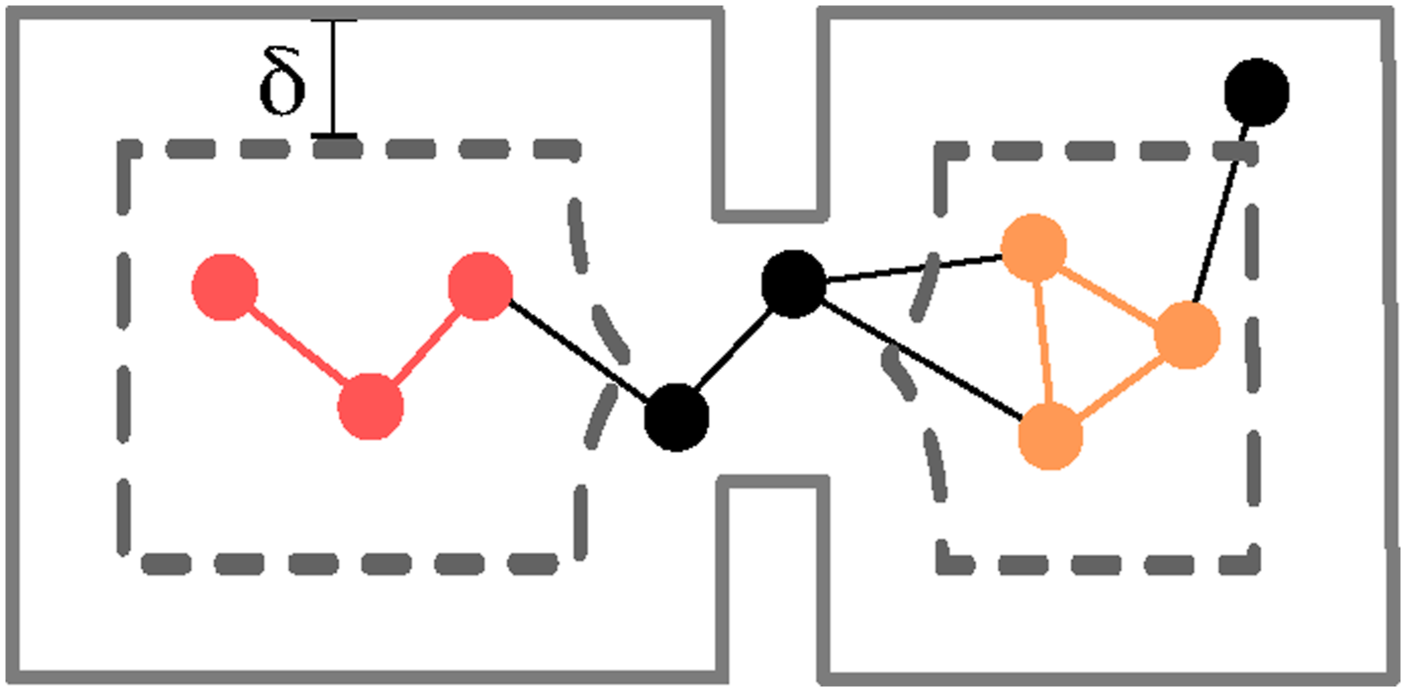

Directly specifying a single best dilation distance δ* to extract putative rooms is unwieldy: door and other aperture widths vary from scene to scene (think about the small doors in an apartment versus large passage ways in a mansion). In order to avoid hard-coding a single dilation distance, we use a tool from topology, known as persistent homology (Ali et al., 2022; Huber 2021), to automatically compute the best dilation distance for a given graph. ¹⁰ The basic insight is that the most natural choice of rooms is one that is more stable (or persistent) across a wide range of dilation distances. To formalize this intuition, the persistent homology literature relies on the notion of filtration. A filtration of a graph ${\mathcal{G}}_p$ is a set of graphs ${\mathcal{G}}_p^{{\delta }_i}$ ordered by real-valued parameters δ _i such that

$\varnothing \subseteq \dots \subseteq {\mathcal{G}}_p^{{\delta }_{i+1}}\subseteq {\mathcal{G}}_p^{{\delta }_i}\subseteq \dots \subseteq {\mathcal{G}}_p.$

(7)

In our case, each graph ${\mathcal{G}}_p^{{\delta }_i}$ is the sub-graph of ${\mathcal{G}}_p$ where nodes and edges with radius smaller than δ _i are removed; ¹¹ hence, the filtration is a set of graphs corresponding to increasing distances δ _i ; see Figure 7(b) and (d) for examples of graphs in the filtration. For each graph in the filtration, we compute the 0-homology (the number of connected components), which in our setup corresponds to the number of rooms the graph gets partitioned into; computationally, the 0-homology can be computed in one shot for all graphs in the filtration by iterating across the edges in the original graph ${\mathcal{G}}_p$ using a union set (Aktas et al., 2019), leading to an extremely efficient algorithm.

Figure 7.

(a) Example of Betti curve; we only consider components with at least 15 nodes. (b–d) Example of filtration of the graph for various thresholds δ. Nodes with distances d ^p smaller than the threshold δ are shown in gray, while nodes with distances above δ are colored by component membership.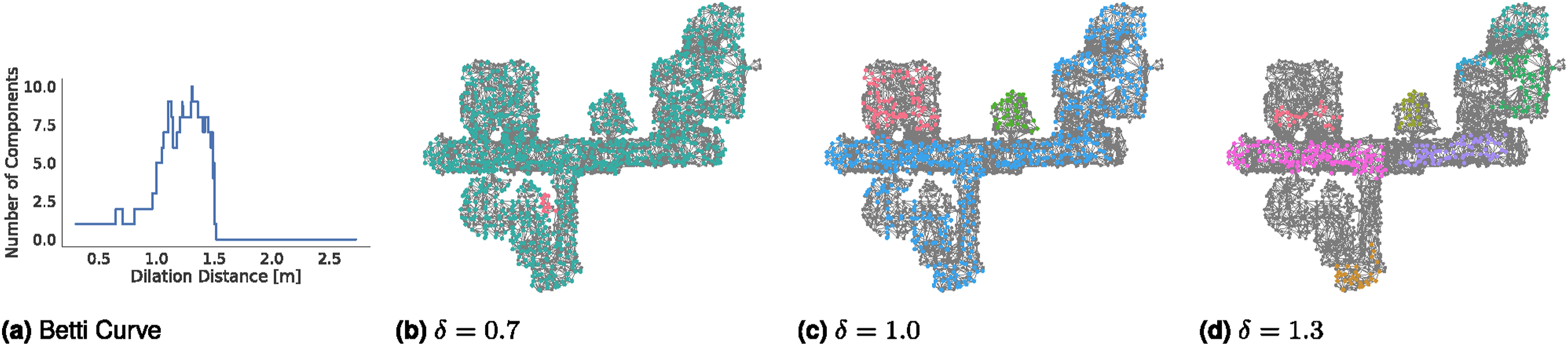

The resulting mapping between the dilation distance and the number of connected components is an example of Betti curve, or β₀(δ); see Figure 7(a) for an example. Intuitively, for increasing distances δ, the graph first splits into more and more connected components (this is the initial increasing portion of Figure 7(a)), and then for large δ entire components tend to disappear (leading to a decreasing trend in the second part of Figure 7(a)), eventually leading to all the nodes disappearing (i.e., zero connected components as shown in the right-most part of Figure 7(a)). In practice, we restrict the set of distances to a range $\left[d^{-},d^{+}\right]$ , containing reasonable sizes for openings between rooms ([0.5, 1.2]m in our tests). We also do not count connected components containing less than a minimum number of vertices (15 in our tests), as we are not interested in segmenting overly small regions as rooms.

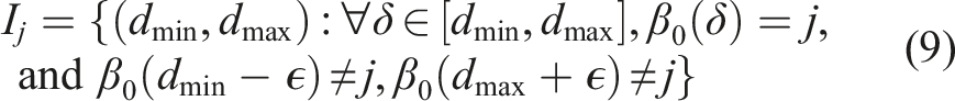
Choices of rooms that are more persistent correspond to large “flat” horizontal regions of the Betti curve, where the number of connected components stays the same across a large sub-set of δ values. More formally, let us denote with H the set of unique values assumed by the Betti curve, i.e.,

$H=\left\{i\mathbb{\in }\mathbb{N}:i={\beta }_0\left(\delta \right),\forall \delta \in \left[d^{-},d^{+}\right]\right\}$

(8)

and—for some small positive constant ϵ—denote with I the set of intervals I _j (for each j ∈ H) defined as

$\begin{array}{l}{I}_j=\{\left(d_{\min },d_{\max }\right):\forall \delta \in \left[d_{\min },d_{\max }\right],{\beta }_0\left(\delta \right)=j,\\ \text{and} {\beta }_0\left(d_{\min }-ϵ\right)\ne j,{\beta }_0\left(d_{\max }+ϵ\right)\ne j\}\end{array}$

(9)

where, for each number of connected components H, the set I contains the extremes (d_min, d_max) of the corresponding flat interval in the Betti curve. Finally, we denote with L the lengths of the intervals in I. Then, the most persistent choice for the number of rooms is the one corresponding to the longest interval in L. In our approach, we choose the number of rooms (and associate an initial set of places to each room) by looking at “sufficiently persistent” intervals (i.e., flat regions with length larger than a threshold). In more detail, we select a subset of L, denoted as $\overline{L}$ , that only contains the intervals of size greater than α ⋅ max_l∈Ll, where α is a user-specified parameter in $\left[0,1\right]$ that balances between over-segmentation (α closer to 0) and under-segmentation (α closer to 1). From these candidates, we assign δ* to be ${\delta }^{*}=d_{\min }^{*}$ , where $\left(d_{\min }^{*},d_{\max }^{*}\right)$ are the extremes of the interval in $\overline{L}$ attaining the largest number of connected components. In other words, we choose the number of rooms to be the largest among all flat intervals that are sufficiently long (i.e., longer than α ⋅ max_l∈Ll). As before, for this choice of δ*, we use the connected components corresponding to that dilation distance as an initial guess for the room clustering. ¹²

3.4.1.2. Assigning remaining nodes via flood-fill

The connected components produced by the persistent homology do not account for all places in ${\mathcal{G}}_p$ , as nodes and edges in the graph disappear depending on the dilation distance. We assign the remaining place nodes to the putative room via the flood-fill algorithm, where the expansion queue is ordered by the distance of each edge to the nearest obstacle, resulting in node connections with the greatest distance to an obstacle being expanded first. This ensures that every node in the places graph ${\mathcal{G}}_p$ is assigned to a room, provided that every original connected component of ${\mathcal{G}}_p$ contains at least one room.

Remark 8

Novelty, Advantages, and Limitations. Many classical 2D room segmentation techniques, such as watershed or morphology approaches, are also connected to persistent homology (Bormann et al. 2016). Our room clustering method provides four key advantages. First, our approach is able to reason over arbitrary 3D environments, instead of a 2D occupancy grid (such as Kleiner et al. (2017)). Second, the approach reasons over a sparse set of places and is extremely computationally and memory efficient in practice; this is in stark contrast with approaches processing monolithic voxel-based maps (e.g., Rosinol et al. (2021) reported runtimes of tens of minutes). Third, the approach automatically computes the dilation distance used to cluster the graph; this allows it to work across a variety of environments (in Section 6, we report experiments in both small apartments and student residences). Fourth, it provides a more solid theoretical framework, compared to the heuristics proposed in related work (Bavle et al. 2022a; Hughes et al. 2022). As a downside, our room clustering approach, similarly to related work relying on geometric reasoning for room segmentation, may fail to segment rooms without a clear geometric footprint, e.g., open floor-plans.

3.4.1.3. Intra-layer and inter-layer edges

We connect pairs of rooms, say (i, j), whenever a place in room i shares an edge with a place in room j. For each room, we add edges to all places in the room. We connect all rooms to a single building node, whose position is the mean of all room centroids.

3.4.2. Layer 4: Room classification via neural tree

While in the previous section, we (geometrically) clustered places nodes into different rooms, the approach described in this section assigns a semantic label (e.g., kitchen, bedroom) to each room. The key insight that we are going to use is that objects in a room are typically correlated with the room type (e.g., a room that contains refrigerator, oven, and toaster is likely to be a kitchen, a room with a bathtub and a toilet is likely to be a bathroom). Edges connecting rooms may also carry information about the room types (e.g., a master bedroom is more likely to be connected to a bathroom). We construct a sub-graph of the 3D scene graph that includes the object and the room layers and the corresponding intra- and inter-layer edges. Given this graph, and the object semantic labels, centroids, and bounding boxes (see Section 3.2), we infer the semantic labels of each room.

While room inference could be attacked via standard techniques for inference in probabilistic graphical models, those techniques typically require handcrafting or estimating expressions for the factors connecting the nodes, inducing a probability distribution over the labels in the graph. We instead rely on more modern techniques that use graph neural networks (GNNs) to learn a suitable neural message passing function between the nodes to infer the missing labels. In particular, room classification can be thought of as a semi-supervised node classification problem (Hamilton. et al., 2017; Kipf and Welling 2017), which has been extensively studied in machine learning. We also observe that our problem has two key features that make it unique. First, the object-room graph is a heterogeneous graph and contains two kinds of nodes, namely objects and rooms, as opposed to large, homogeneous social network graphs (one of the key benchmarks applications in the semi-supervised node classification literature). Second, the object-room graph is a hierarchical graph (Definition 1), which gives more structure to the problem (e.g., Proposition 6). ¹³ We review a recently proposed GNN architecture, the neural tree (Talak et al., 2021), that takes advantage of the hierarchical structure of the graph and leads to (provably and practically) efficient and accurate inference.

3.4.2.1. Neural tree overview

While traditional GNNs perform neural message passing on the edges of the given graph $\mathcal{G}$ (the object-room graph in our case), the key idea behind the neural trees architecture is to construct a tree-structured graph from the input graph and perform message passing on the resulting tree instead of the input graph (Talak et al., 2021). This tree-structured graph, the H-tree, is similar to a tree decomposition, and is such that every node in it represents either a node or a subset of nodes in the input graph. Trees are known to be more amenable for message passing (e.g., the junction tree algorithm enables exact inference for graphs with small treewidth) (Jordan 2002; Koller and Friedman 2009). Analogously, the neural tree has been shown to enable strong approximation results (Talak et al., 2021) and lead to better classification accuracy in practice (see Talak et al. (2021) and Section 6). We briefly review the construction of the H-tree, the choice of message passing, and the resulting performance guarantees, and we refer the reader to Talak et al. (2021) for an in-depth discussion.

3.4.2.2. Constructing the H-Tree

The neural tree performs message passing on the H-tree, a tree-structured graph constructed from the input graph. Each node in the H-tree corresponds to a sub-graph of the input graph. These sub-graphs are arranged hierarchically in the H-tree such that the parent of a node in the H-tree always corresponds to a larger sub-graph in the input graph. The leaf nodes in the H-tree correspond to singleton subsets (i.e., individual nodes) of the input graph.

The first step to construct an H-tree is to compute a tree decomposition T of the object-room graph. Since the object-room graph is a hierarchical graph, we use Algorithm 1 to efficiently compute a tree decomposition. The bags in such a tree decomposition contain either (A) only room nodes, (B) only object nodes, or (C) object nodes with one room node. To form the H-tree, we need to further decompose the leaves of the tree decomposition into singleton nodes. For bags falling in the cases (A)-(B), we further decompose the bags using a tree decomposition of the sub-graphs formed by nodes in the bag, as described in Talak et al. (2021). For case (C), we note that the sub-graph is again a hierarchical graph with one room node, hence we again use Algorithm 1 to compute a tree decomposition. We form the H-tree by concatenating these tree decompositions hierarchically as described in Talak et al. (2021).

3.4.2.3. Message passing and node classification

Message passing on the H-tree generates embeddings for all the nodes and important sub-graphs of the input graph. Any of the existing message passing protocols (e.g., the ones used in Graph Convolutional Networks (GCN) (Bronstein et al., 2017; Defferrard et al., 2016; Henaff et al., 2015; Kipf and Welling 2017; Kipf and Welling 2017, 2017), GraphSAGE (Hamilton. et al., 2017), or Graph Attention Networks (GAT) (Busbridge et al., 2019; Lee et al., 2019; Veličković et al., 2018)) can be re-purposed to operate on the neural tree. We provide an ablation of different choices of message passing protocols and node features in Section 6. After message passing is complete, the final label for each node is extracted by pooling embeddings from all leaf nodes in the H-tree corresponding to the same node in the input graph, as in Talak et al. (2021).

One important difference between the H-tree in Talak et al. (2021), and the H-tree constructed for the object-room graph is the heterogeneity of the latter. The H-tree of a heterogeneous graph will also be heterogeneous, i.e., the H-tree will now contain nodes that correspond to various kinds of sub-graphs in the input object-room graph. Specifically, the H-tree has nodes that correspond to sub-graphs: (i) containing only room nodes, (ii) containing one room node and multiple object nodes, (iii) containing only object nodes, and (iv) leaf nodes which correspond to either an object or a room node. Accordingly, we treat the neural tree as a heterogeneous graph when performing message passing. Message passing over heterogeneous graphs can be implemented using off-the-shelf functionalities in the PyTorch geometric library (Fey and Lenssen 2019).

3.4.2.4. Expressiveness of the neural tree and graph treewidth

The following result, borrowed from our previous work (Talak et al., 2021), establishes a connection between the expressive power of the neural tree and the treewidth of the corresponding graph.

Theorem 9

Neural Tree Expressiveness, Theorem 7 and Corollary 8 in Talak et al. (2021). Call $\mathcal{F}\left(\mathcal{G},N\right)$ the space of functions that can be produced by applying the neural tree architecture with N parameters to the graph $\mathcal{G}$ . Let f : [0,1] ⁿ → [0, 1] be a function compatible with a graph $\mathcal{G}$ with n nodes, i.e., a function that can be written as $f\left(\mathit{X}\right)={\sum }_{C\in \mathcal{C}\left(\mathcal{G}\right)}{\theta }_C\left({\mathit{x}}_C\right)$ , where $\mathcal{C}\left(\mathcal{G}\right)$ denotes the collection of all maximal cliques in $\mathcal{G}$ and θ _C is some function that maps features associated to nodes in a clique C to a real number. Let each clique function θ _c in f be 1-Lipschitz and be bounded to [0, 1]. Then, for any ϵ > 0, there exists a function $g\in \mathcal{F}\left(\mathcal{G},N\right)$ such that ‖f − g‖ _∞ < ϵ, while the number of parameters N is bounded by

$N=\mathcal{O}\left(n\times {\left(\text{tw}\left[{\mathcal{J}}_{\mathcal{G}}\right]+1\right)}^{2\text{tw}\left[{\mathcal{J}}_{\mathcal{G}}\right]+3}\times {ϵ}^{-\left(\text{tw}\left[{\mathcal{J}}_{\mathcal{G}}\right]+1\right)}\right),$

(10)

where $\text{tw}\left[{\mathcal{J}}_{\mathcal{G}}\right]$ denotes the treewidth of the tree decomposition of $\mathcal{G}$ , computed according to Algorithm 1.

While we refer the reader to Talak et al. (2021) for a more extensive discussion, the intuition is that graph-compatible functions can model (the logarithm of) any probability distribution over the given graph. Hence, Theorem 9 essentially states that the neural tree can learn any (sufficiently well-behaved) graphical model over $\mathcal{G}$ , with a number of parameters that scales exponentially in the graph treewidth, and only linearly in the number of nodes in the graph. Therefore, for graphs with small treewidth (as the ones of Proposition 6), we can approximate arbitrary relations between the nodes without requiring too many parameters. Furthermore, Proposition 6 and Proposition 3 ensure that we can compute the tree decomposition (and hence the H-tree) efficiently in practice. Beyond these theoretical results, in Section 6 we show that the use of the neural tree leads to improved accuracy in practice.

4. Persistent representations: Detecting and enforcing loop closures in 3D scene graphs

The previous section discussed how to estimate the layers of an “odometric” 3D scene graph as the robot explores an unknown environment. In this section, we discuss how to use the 3D scene graph to detect loop closures (Section 4.1), and how to correct the entire 3D scene graph in response to putative loop closures (Section 4.2).

4.1. Loop closure detection and geometric verification

We augment visual loop closure detection and geometric verification by using information across multiple layers in the 3D scene graph. Standard approaches for visual place recognition rely on visual features (e.g., SIFT, SURF, ORB) and fast retrieval methods (e.g., bag of words (Gálvez-López and Tardós 2012)) to detect loop closures. Advantageously, the 3D scene graph not only contains visual features (included in each node of the agent layer), but also additional information about the semantics of the environment (described by the object layer) and the geometry and topology of the environment (described by the places layer). In the following we discuss how to use this additional 3D information to develop better descriptors for loop closure detection and geometric verification.

4.1.1. Top-down loop closure detection

As mentioned in Section 3.2, the agent layer stores visual features for each keyframe pose along the robot trajectory. We refer to each such poses as agent nodes. Loop closure detection then aims at finding a past agent node that matches (i.e., observes the same portion of the scene seen by) the latest agent node, which corresponds to the current robot pose.

4.1.1.1. Top-down loop closure detection overview

For each agent node, we construct a hierarchy of descriptors describing statistics of the node’s surroundings, from low-level appearance to semantics and geometry. At the lowest level, our hierarchical descriptors include standard DBoW2 appearance descriptors (Gálvez-López and Tardós 2012). We augment the appearance descriptor with an object-based descriptor and a place-based descriptor computed from the objects and places in a sub-graph surrounding the agent node. We provide details about two choices of descriptors (hand-crafted and learning-based) below. To detect loop closures, we compare the hierarchical descriptor of the current (query) node with all the past agent node hierarchical descriptors, searching for a match. When comparing descriptors, we walk down the hierarchy of descriptors (from places, to objects, to appearance descriptors). In particular, we first compare the places descriptor and—if the descriptor distance is below a threshold—we move on to comparing object descriptors and then appearance descriptors. If any of the appearance or object descriptor comparisons return a strong enough match (i.e., if two distance between two descriptors is below a threshold), we perform geometric verification; see Figure 8 for a summary.

Figure 8.

Loop closure detection (left) and geometric verification (right). To find a match, we “descend” the 3D scene graph layers, comparing descriptors. We then “ascend” the 3D scene graph layers, attempting registration.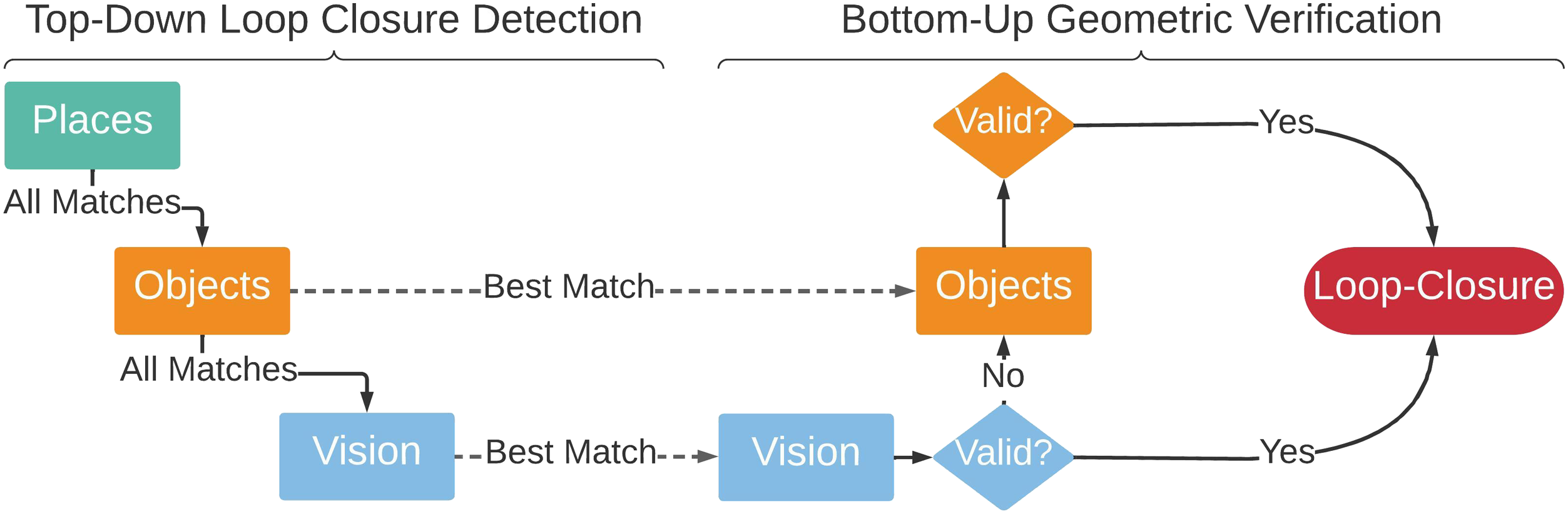

4.1.1.2. Hand-crafted scene graph descriptors

Top-down loop closure detection relies on having descriptors (i.e., vector embeddings) of the sub-graphs of objects and places around each agent node. In the conference version (Hughes et al., 2022) of this paper, we proposed hand-crafted descriptors. In particular, for the objects, we use the histogram of the semantic labels of the object nodes in the sub-graph as an object-level descriptor. For the places, we use the histogram of the distances associated to each place node in the sub-graph as a place-level descriptor. As shown in Hughes et al. (2022) and confirmed in Section 6, the resulting hierarchical descriptors already lead to improved loop closure detection performance over traditional appearance-based loop closures. However, these descriptors fail to capture relevant information about objects and places, e.g., their spatial layout and connectivity. In the following, we describe learning-based descriptors that use graph neural networks to automatically find a suitable embedding for the object and place sub-graphs; these are observed to further improve loop closure detection performance in some cases; see Section 6.

4.1.1.3. Learning-based scene graph descriptors

Given a sub-graph of objects and places around the agent node, we learn fixed-size embeddings using a Graph Neural Network (GNN). At a high level, we learn such embeddings from scene graph datasets, such that the Euclidean distance between descriptors is smaller if the corresponding agent nodes are spatially close.

In more detail, we learn separate embeddings for the sub-graph of objects and the sub-graph of places. For every object layer sub-graph, we encode the bounding-box size and semantic label of each object as node features. For every places layer sub-graph, we encode the distance of the place node to the nearest obstacle and the number of basis points of the node as node features. Rather than including absolute node positions in the respective node features, we assign a weight to each edge (i, j) between nodes i and j as $w_{ij}=e^{-\Vert x_i-x_j\Vert }$ , where x _i and x _j are the positions of nodes i and j. This results in a weight in the range [0, 1], where the closer two nodes are, the higher the edge weight. Associating intra-node distances to edges (rather than using absolute positions as node features) makes the resulting embedding pose-invariant; this is due to the fact that the node positions only enter the network in terms of their distance, which is invariant to rigid transformations. Our GNN model architecture follows the graph embedding architecture presented in Li et al. (2019), which consists of multi-layer perceptrons as encoders for node and edge features, message passing layers, and a graph-level multi-level perception to aggregate node embeddings into the final graph embedding. We use triplet loss (Li et al., 2019) to train the models and defer the details of constructing triplets and other model and training parameters to the experiments in Section 6.

4.1.2. Bottom-up geometric verification

After we have a putative loop closure between our query and match agent nodes (say i and j), we attempt to compute a relative pose between the two by performing bottom-up geometric verification. Whenever we have a match at a given layer (e.g., between appearance descriptors at the agent layer, or between object descriptors at the object layer), we attempt to register frames i and j. For registering visual features we use standard RANSAC-based geometric verification as in Rosinol et al. (2020a). If that fails, we attempt registering objects using TEASER++ (Yang et al., 2020), discarding loop closures that also fail object registration. This bottom-up approach has the advantage that putative matches that fail appearance-based geometric verification (e.g., due to viewpoint or illumination changes) can successfully lead to valid loop closures during the object-based geometric verification. Section 6 shows the proposes hierarchical descriptors improve the quality and quantity of detected loop closures.

4.2. 3D scene graph optimization

This section describes a framework to correct the entire 3D scene graph in response to putative loop closures. Assume we use the algorithms in Section 3 to build an “odometric” 3D scene graph, which drifts over time as it is built from the odometric trajectory of the robot—we refer to this as the frontend (or odometric) 3D scene graph. Then, our goals here are (i) to optimize all layers in the 3D scene graph in a consistent manner while enforcing the detected loop closures (Section 4.1), and (ii) to post-processes the results to remove redundant sub-graphs corresponding to the robot visiting the same location multiple times. The resulting 3D scene graph is what we call a backend (or optimized) 3D scene graph, and we refer to the module producing such a graph as the scene graph backend. Below, we describe the two main processes implemented by the scene graph backend: a 3D scene graph optimization (which simultaneously corrects all layers of the scene graph by optimizing a sparse subset of variables), and an interpolation and reconciliation step (which recovers the dense geometry and removes redundant variables); see Figure 9.

Figure 9.

Loop closure detection and optimization: (a) after a loop closure is detected, (b) we extract and optimize a sub-graph of the 3D scene graph—the deformation graph—that includes the agent poses, the places, and a subset of the mesh vertices. (c) We then reconstruct the rest of the graph via interpolation as in Sumner et al. (2007), and (d) reconcile overlapping nodes.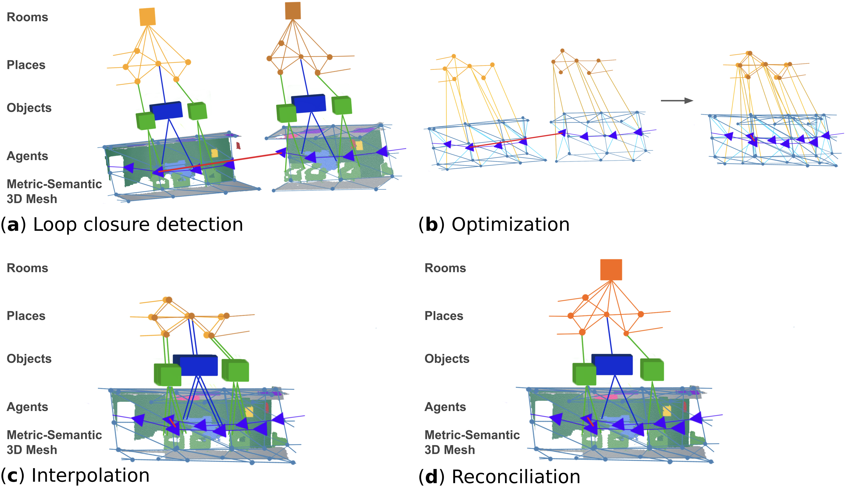

4.2.1. 3D scene graph optimization

We propose an approach to simultaneously deform the 3D scene graph layers using an embedded deformation graph (Sumner et al., 2007). This approach generalizes the pose graph and mesh optimization approach in Rosinol et al. (2021) as it also includes the graph of places in the optimization. At a high-level, the backend optimizes a sparse graph (the embedded deformation graph) built by downsampling the nodes in the 3D scene graph, and then reconstructs the other nodes in the scene graph via interpolation as in Sumner et al. (2007).

Specifically, we form the deformation graph as the sub-graph of the 3D scene graph that includes (i) the agent layer, consisting of a pose graph that includes both odometry and loop closures edges, (ii) the 3D mesh control points, i.e., uniformly subsampled vertices of the 3D mesh (obtained using the same spatial hashing process described in Section 3.1), with edges connecting control points closer together than a distance (2.5 m in our implementation); (iii) a minimum spanning tree of the places layer. ¹⁴ By construction, these three layers form a connected sub-graph (recall the presence of the inter-layer edges discussed in Section 3).

The embedded deformation graph approach associates a local frame (i.e., a pose) to each node in the deformation graph and then solves an optimization problem to adjust the local frames in a way that minimizes deformations associated to each edge (including loop closures). Let us call ${\mathcal{T}}_a$ , ${\mathcal{T}}_m$ , ${\mathcal{T}}_p$ the set of poses associated with the agent layer, the mesh control points, and the places. The poses in ${\mathcal{T}}_a$ are initially set to be the odometric poses of the robot; the poses in ${\mathcal{T}}_m$ are initially set to have identity rotation and translation equal to the mesh control points’ positions; similarly, the poses in ${\mathcal{T}}_p$ are initially set to have identity rotation, and translation equal to the position of the corresponding places. Each edge represents a relative pose or a relative position measurement between pair of poses. In particular, the set of edges is $\mathcal{E}={\mathcal{E}}_{aa}\cup {\mathcal{E}}_{mm}\cup {\mathcal{E}}_{pp}\cup {\mathcal{E}}_{am}\cup {\mathcal{E}}_{ap}\cup {\mathcal{E}}_{mp}$ , where each subset denotes intra-layer edges (e.g., ${\mathcal{E}}_{aa}$ contains the edges within the agent layer), or inter-layer edges (e.g., ${\mathcal{E}}_{am}$ contains the edges between a robot pose and a mesh control point). ¹⁵ Intuitively, the proposed 3D scene graph optimization finds the set of poses that minimizes the mismatch with respect to these relative measurements: a small mismatch corresponds to small deformations of the local geometry of the scene graph and encourages small errors for the loop closure edges.

We can find an optimal configuration for the poses $\mathcal{T}={\mathcal{T}}_a\cup {\mathcal{T}}_m\cup {\mathcal{T}}_p$ in the deformation graph by solving the following optimization problem:

${\mathcal{T}}^{\star }=\underset{\mathit{T}1,\mathit{T}2,\dots \in \mathcal{T}}{\arg \hspace{0.17em}\min }{\displaystyle \sum }_{\left(i,j\right)\in \mathcal{E}}{\Vert \mathit{T}{i}^{-1}\mathit{T}j-\mathit{E}ij\Vert }_{\mathbf{\Omega }ij}^2$

(11)

where T _i ∈ SE(3) and T _j ∈ SE(3) are pairs of 3D poses in $\mathcal{T}$ , E _ij is the relative measurement associated to each edge $\left(i,j\right)\in \mathcal{E}$ (written as a 3D pose), and for a matrix M we use the notation ${\Vert \mathit{M}\Vert }_{\mathbf{\Omega }}^2\triangleq \text{tr}\left(\mathit{M}\mathrm{\Omega }{\mathit{M}}^{\mathsf{T}}\right)$ . ¹⁶ The 4 × 4 positive semidefinite matrix Ω _ij is chosen as the inverse of the odometry (or loop closure) covariances for the edges in ${\mathcal{E}}_{aa}$ , while it is set to diag  [0 0 0 ω _t ] for the other relative position measurements, where the zeros cancel out the rotation component of the residual error T _i ⁻¹T _j − E _ij , and ω _t is a user-specified parameter that controls how much deformation we want to allow for each edge during the optimization. ¹⁷

In hindsight, 3D scene graph optimization transforms a subset of the 3D scene graph into a factor graph (Cadena et al., 2016), where edge potentials need to be minimized. The expert reader might also realize that (11) is mathematically equivalent to standard pose graph optimization in SLAM (Cadena et al., 2016), which enables the use of established off-the-shelf solvers. In particular, we solve (11) using the Graduated Non-Convexity (GNC) solver in GTSAM (Antonante et al., 2021), which is also able to reject incorrect loop closures as outliers.

4.2.2. Interpolation and reconciliation

Once the optimization terminates, the agent and place nodes are updated with their new (optimized) positions and the full mesh is interpolated back from its control points according to the deformation graph approach in Sumner et al. (2007); Rosinol et al. (2021). After the 3D scene graph optimization and the interpolation step, certain portions of the scene graph—corresponding to areas revisited multiple times by the robot—contain redundant information. To avoid this redundancy, we merge overlapping nodes. For places nodes, we merge nodes within a distance threshold (0.4 m in our implementation). For object nodes we merge nodes if the corresponding objects have the same semantic label and if one of nodes is contained inside the bounding box of the other node. After this process is complete, we recompute the object centroids and bounding boxes from the position of the corresponding vertices in the optimized mesh. Finally, we recompute the rooms from the graph of places using the approach in Section 3.4.

5. Thinking fast and slow: The Hydra architecture

We integrate the algorithms described in this paper into a highly parallelized spatial perception system, named Hydra. Hydra involves a combination of processes that run at sensor rate (e.g., feature tracking for visual-inertial odometry), at sub-second rate (e.g., mesh and place reconstruction, object bounding box computation), and at slower rates (e.g., the scene graph optimization, whose complexity depends on the map size). Therefore these processes have to be organized such that slow-but-infrequent computation (e.g., scene graph optimization) does not get in the way of faster processes.

We visualize Hydra in Figure 10. Each block in the figure denotes an algorithmic module, matching the discussion in the previous sections. Hydra starts with fast early perception processes (Figure 10, left), which perform low-level perception tasks such as feature detection and tracking (required for visual-inertial odometry, and executed at frame-rate), 2D semantic segmentation, and stereo-depth reconstruction (at keyframe rate). The result of early perception processes are passed to mid-level perception processes (Figure 10, center). These include algorithms that incrementally construct (an odometric version of) the agent layer (e.g., the visual-inertial odometry backend), the mesh and places layers, and the object layer. Mid-level perception also includes the scene graph frontend, which is a module that collects the result of the other modules into an “unoptimized” scene graph. Finally, the high-level perception processes perform loop closure detection, execute scene graph backend optimization, and extract rooms (including both room clustering and classification). ¹⁸ This results in a globally consistent, persistent 3D scene graph.

Figure 10.

Hydra’s functional blocks. We conceptualize three different functional block groupings: low-level perception, mid-level perception, and high-level perception in order of increasing latency. Each functional block is labeled with a number that identifies the “logical” thread that the module belongs to.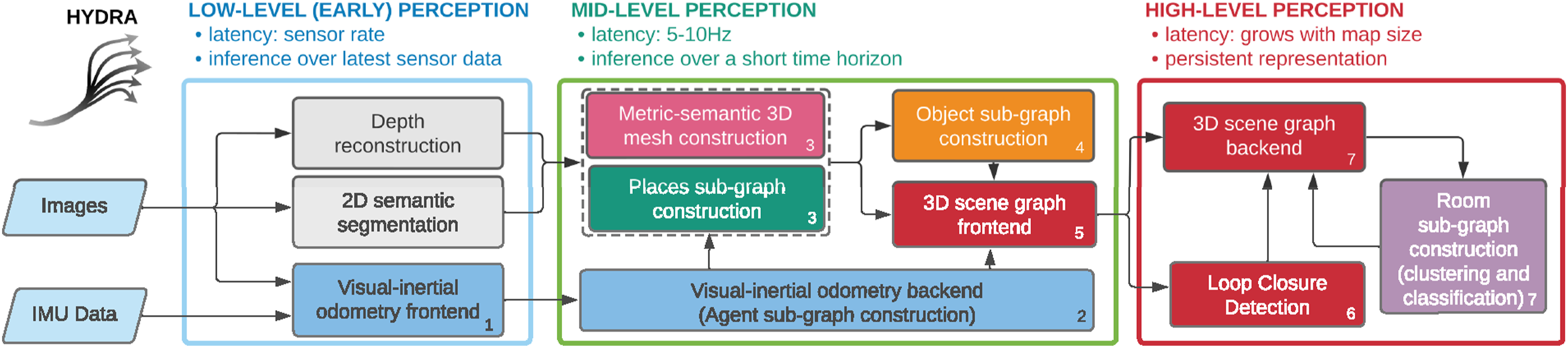

Hydra runs in real-time on a multi-core CPU. The only module that relies on GPU computing is the 2D semantic segmentation, which uses a standard off-the-shelf deep network. The neural tree (Section 3.4.2) and the GNN-based loop closure detection (Section 4.1) can be optionally executed on a GPU, but the forward pass is relatively fast even on a CPU (see Section 6.3.4). The fact that most modules run on CPU has the advantage of (i) leaving the GPU to learning-oriented components, and (ii) being compatible with the power limitations imposed by current mobile robots. In the next section, we will report real-time results with Hydra running on a mobile robot, a Unitree A1 quadruped, with onboard sensing and computation (an NVIDIA Xavier embedded computer).

6. Experiments

The experiments in this section (i) qualitatively and quantitatively compare the 3D scene graph produced by Hydra to another state-of-the-art 3D scene graph construction method, SceneGraphFusion (Wu et al., 2021), (ii) examine the performance of Hydra in comparison to batch offline methods, i.e., Kimera (Rosinol et al., 2021), (iii) validate design choices for learned components in our method via ablation studies, and (iv) present a runtime analysis of Hydra. We also document our experimental setup, including training details for both the GNN-based loop closure descriptors and the neural-tree room classification, and datasets used. Our implementation of Hydra is available at https://github.com/MIT-SPARK/Hydra.

6.1. Datasets

We use four primary datasets for training and evaluation: two simulated datasets (Matterport3D (Chang et al., 2017) and uHumans2 (Rosinol et al., 2021)) and two real-world datasets (SidPac and Simmons). In addition, we use the Stanford3D dataset (Armeni et al., 2019) to motivate neural tree design choices with respect to our initial proposal in Talak et al. (2021). Note that Matterport3D ¹⁹ , uHumans ²⁰ , and Stanford3D ²¹ are all publicly available.

6.1.1. Matterport3D

We utilize the Matterport3D (MP3D) dataset (Chang et al., 2017), an RGB-D dataset consisting of 90 reconstructions of indoor building-scale scenes. We use the Habitat Simulator (Savva et al., 2019) to traverse the scenes from the MP3D dataset and render color imagery, depth, and ground-truth 2D semantic segmentation. We generate two different 3D scene graphs datasets for the 90 MP3D scenes by running Hydra on pre-generated trajectories; one for training descriptors and one for room classification. For training the GNN-based descriptors for loop closure detection (GNN-LCD), we generate a single trajectory for each scene through the navigable scene area such that we get coverage of the entire scene, resulting in 90 scene graphs. For training the room classification approaches, we generate 5 trajectories for each scene by randomly sampling navigable positions until a total path length of at least 100 m is reached, resulting in 450 trajectories. When running Hydra on these 450 trajectories, we save intermediate scene graphs every 100 timesteps (resulting in roughly 15 scene graphs per trajectory), giving us 6810 total scene graphs.

6.1.2. uHumans2

The uH2 dataset is a Unity-based simulated dataset (Rosinol et al., 2021) that includes four scenes: a small apartment, an office, a subway station, and an outdoor neighborhood. For the purposes of this paper, we only use the apartment and office scenes. The dataset provides visual-inertial data, ground-truth depth, and 2D semantic segmentation. The dataset also provides ground truth trajectories that we use for benchmarking.

6.1.3. SidPac

The SidPac dataset is a real dataset collected in a graduate student residence using a visual-inertial hand-held device. We used a Kinect Azure camera as the primary collection device, providing color and depth imagery, with an Intel RealSense T265 rigidly attached to the Kinect to provide an external odometry source. The dataset consists of two separate recordings, both of which are used in our previous paper Hughes et al. (2022). We only use the first recording for the purposes of this paper. This first recording covers two floors of the building (Floors 1 & 3), where we walked through a common room, a music room, and a recreation room on the first floor of the graduate residence, went up a stairwell, through a long corridor as well as a student apartment on the third floor, then finally down another stairwell to revisit the music room and the common room, ending where we started. These scenes are particularly challenging given the scale of the scenes (average traversal of around 400 m), the prevalence of glass and strong sunlight in regions of the scenes (causing partial depth estimates from the Kinect), and feature-poor regions in hallways. We obtain a proxy for the ground-truth trajectory for the Floor 1 & 3 scene via a hand-tuned pose graph optimization with additional height priors, to reduce drift and qualitatively match the building floor plans.

6.1.4. Simmons

The Simmons dataset is a real dataset collected on a single floor of an undergraduate student residence with a Clearpath Jackal rover and a Unitree A1 quadruped robot (Figure 11). The Clearpath Jackal rover uses the RealSense D455 camera as the primary collection device to provide color and depth imagery, but the rover is also equipped with a Velodyne to perform LIDAR-based odometry (Reinke et al., 2022) as an external odometry source. The A1 also uses the RealSense D455 camera as the primary collection device, but is not equipped with a Velodyne; instead, it is equipped with an industrial grade Microstrain IMU to improve the performance of the visual-inertial odometry (Rosinol et al., 2020a). The dataset consists of two recordings, one recorded on the Jackal, and one recorded using the A1. The Jackal recording covers the rooms scattered throughout half of a single floor of the building, where the Jackal traverses a distance of around 500 m through mostly student bedrooms, but also a lounge area, a kitchen, and a laundry room; the rooms are all joined by a long hallway that spans the full floor. The A1 sequence takes place on one end of the floor and maps 4 bedrooms, a small lounge, and a section of the hallway that connects all the rooms. The dataset is challenging due to the visual and structural similarity across student rooms that have similar layouts and furnishing. We obtain a proxy for the ground-truth trajectory for the Jackal using LIDAR-based SLAM, by running LOCUS (Reinke et al., 2022) with flat ground assumption and LAMP (Chang et al., 2022) for loop closure corrections. The ground-truth trajectory of the A1 is obtained by registering individual visual keyframes with the visual keyframes in the Jackal sequence, and then corrected using the proxy ground-truth of the Jackal sequence.

Figure 11.

(a) The Clearpath Jackal platform used to record one of the Simmons sequences. The Jackal is equipped with both a RealSense D455 camera and a Velodyne LIDAR. (b) The Unitree A1 platform used to record the second Simmons sequence. The A1 is equipped with a RealSense D455 camera and a Microstrain IMU. Both platforms have an Nvidia Xavier NX embedded computer onboard.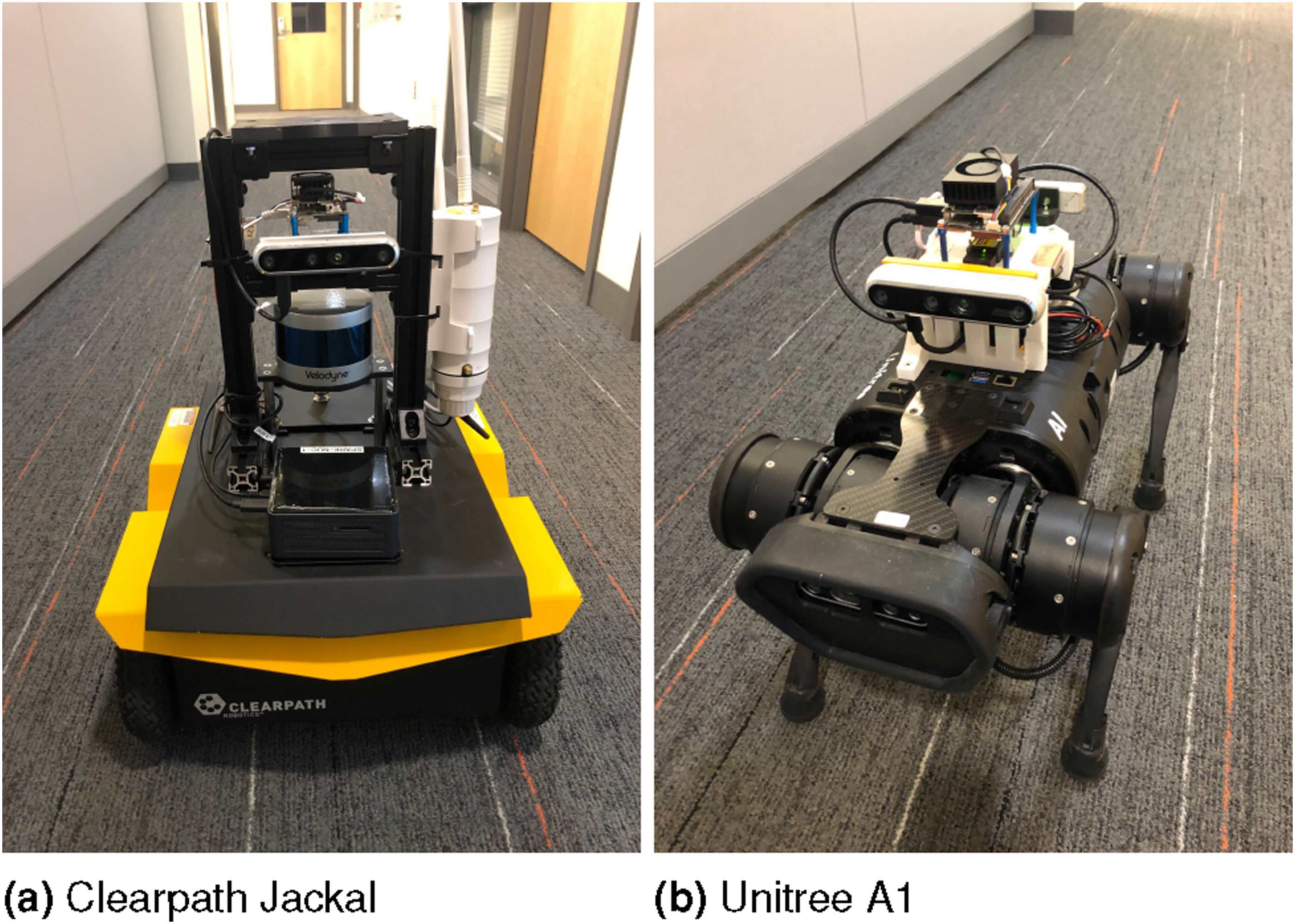

6.1.5. Stanford3D

We use the 35 human-verified scene graphs from the Stanford 3D Scene Graph (Stanford3d) dataset (Armeni et al., 2019) to compare the neural tree against standard graph neural networks for node classification and to assess new design choices against our initial proposal in Talak et al. (2021). These scene graphs represent individual residential units, and each consists of building, room, and object nodes with inter-layer connectivity. We use the same pre-processed graphs as in Talak et al. (2021) where the single-type building nodes (residential) are removed and additional 4920 intra-layer object edges are added to connect nearby objects in the same room. This results in 482 room-object graphs, each containing one room and at least one object per room. The full dataset has 482 room nodes with 15 semantic labels, and 2338 objects with 35 labels.

6.2. Experimental setup

In this section, we first discuss the implementation of Hydra, including our choice of networks for the 2D semantic segmentation. Then we provide details regarding the training of our learning-based approaches: the GNN-LCD descriptors and the neural tree for room classification.

6.2.1. Hydra

To provide 2D semantic segmentation for the real-world datasets, we compare three different models, all of which use the ADE20k (Zhou et al., 2017) label space. We use HRNet (Wang et al., 2021) as a “nominal” semantic segmentation source and MobileNetV2 (Sandler et al., 2018) as a light-weight source of semantics for use on a robot. For both HRNet and MobileNetV2, we use the pre-trained model from the MIT Scene Parsing challenge (Zhou et al., 2017) to export a deployable model for our inference toolchain (ONNX and TensorRT). Additionally, we use a state-of-the-art model, OneFormer (Jain et al., 2023), to provide more-accurate-but-slower 2D semantic segmentation. A comparison of the accuracy and frame-rate of these models is shown in Figure 12.

Figure 12.

(a) A sample RGB image from SidPac Floor 1-3. (b–d) 2D semantic segmentation from OneFormer (Jain et al., 2023), HRNet (Wang et al., 2021), and MobileNetV2 (Sandler et al., 2018). The framerate of each approach is overlaid on the images for both the GPU in the workstation used for evaluation (an Nvidia GTX 3080), as well as for a less powerful embedded computer (the Nvidia Xavier NX). OneFormer was not tested on the Xavier NX.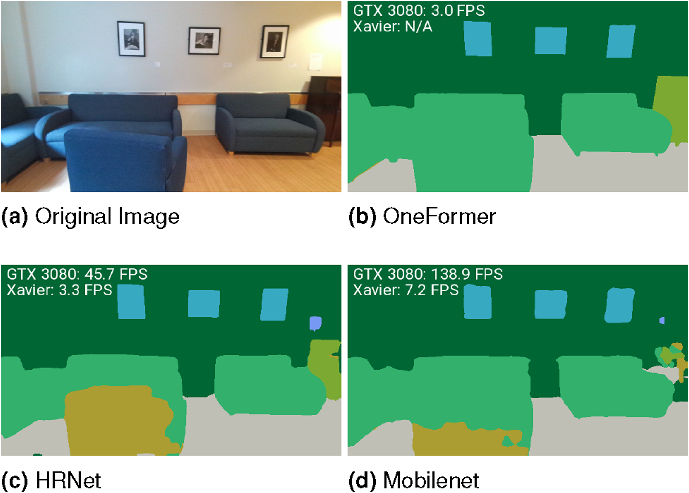

For both simulated and real datasets we use Kimera-VIO (Rosinol et al., 2020a) for visual-inertial odometry. For SidPac, we fuse the Kimera-VIO estimates with the output of the RealSense T265 to improve the quality of the odometric trajectory. For Simmons, we fuse the Kimera-VIO estimates with the odometry output of Reinke et al. (2022) to improve the quality of the odometric trajectory for the sequence recorded by the Jackal platform.

All the remaining blocks in Figure 10 are implemented in C++, following the approach described in this paper. In the experiments we primarily use a workstation with an AMD Ryzen9 3960X with 24 cores and two Nvidia GTX3080s. We also report timing results on an embedded computer (Nvidia Xavier NX) at the end of this section, and demonstrate the full Hydra system running on the same embedded computer onboard the A1 robot; see the video attachment.

6.2.2. GNN-LCD training

We use the MP3D scene graphs to train loop closure descriptors for the object and place sub-graphs. We generate a sub-graph around every agent pose which consists of all nodes and edges within a provided radius of the parent place node that the agent pose is nearest to. We adaptively determine the radius for each sub-graph; each sub-graph has a minimum radius of 3 m and is grown until either a minimum number of nodes (10) or a maximum radius of 5 m is reached. Each object and place sub-graph contains the node and edges features as described in Section 4.1. The semantic label of each object node is encoded either using word2vec (Mikolov et al., 2013) or a one-hot encoding. We explore the impact of this label encoding in Section 6.3.

We use triplet loss to train our model. To construct the triplets, we have an anchor (a candidate sub-graph), and need to find positive and negative examples to compute the loss. A good proxy for how similar two sub-graphs are is looking at the spatial overlap of the two sets of nodes of the sub-graphs. We compute this overlap between the sub-graphs by using IoU over the bounding boxes that encompass the positions of the nodes of each sub-graph. If the overlap between two sub-graphs is at least 40%, we consider them to be similar (and candidates for positive examples), otherwise they are considered negative examples for that particular anchor. Sub-graphs from different scenes are always considered negative examples. To train our GNN-LCD descriptors, we use online triplet mining with batch-all triplet loss (Schroff et al., 2015), where we construct valid triplets for a batch of sub-graph input embeddings and average loss on the triplets that produce a positive loss.

The message-passing architecture that we selected is GCNConv (Kipf and Welling 2017). While more expressive or performant architectures exist, few are compatible with the computational framework used for inference in Hydra (i.e., ONNX). We split the dataset by scene; we use 70% of the original 90 scene graphs to train on, 20% of the scene graphs for validation, and the last 10% for testing. Our learning rate is 5 × 10⁻⁴, and we train the object models for 50 epochs and place models for 80 epochs, saving the model when the average validation error is at a minimum. Each model produces a descriptor of dimension 64. Other key model parameters are reported in Appendix A.7.

6.2.3. Neural tree training

We train the neural tree and related baselines on two datasets: Stanford3d and MP3D.

For the 482 object-room scene graphs in the Stanford3D dataset, we train the neural tree and GNN baselines for the same semi-supervised node classification task examined in (Talak et al., 2021), where the architecture has to label a subset of room and object nodes. The goal of this comparison is to understand the impact of some design choices (e.g., heterogeneous graphs, edge features) with respect to our original proposal in (Talak et al., 2021) and related work. For this comparison, we implement the neural tree and baseline approaches with four different message passing functions: GCN (Kipf and Welling 2017), GraphSAGE (Hamilton et al., 2017), GAT (Veličković et al., 2018), and GIN (Xu et al., 2019b). We consider both homogeneous and heterogeneous graphs; for all nodes, we use their centroid and bounding box size as node features. In some of our comparisons, we also examine the use of relative node positions as edge features, and discard the centroid from the node features. For the GNN baselines, we construct heterogeneous graphs consisting of two node types: rooms and objects. For the neural tree, we obtain graphs with four node types: room cliques, room-object cliques, room leaves, and object leaves; see Section 3.4.2. There are few message passing functions that are compatible with both heterogeneous graphs and edge features; therefore, we compare all heterogeneous approaches using only GAT (Veličković et al., 2018). For all tests on Stanford3d, we report average test accuracy over 100 runs. For each run, we randomly generate a 70%, 10%, 20% split across all nodes (i.e., objects and rooms) for training, validation, and testing, respectively.

For the 6180 scene graphs in the MP3D dataset, we test the neural tree and baselines for room classification on object-room graphs. The goal of this experiment is to understand the impact of the node features and the connectivity between rooms on the accuracy of room classification. We only consider heterogeneous graphs for this dataset, and as such only use GAT (Veličković et al., 2018) for message passing. The heterogeneous node types are the same as for Stanford3D. We use the bounding box size as the base feature for each node, and use relative positions between centroids as edge features. We also evaluate the impact of using semantic labels as additional features for the object nodes using word2vec (Mikolov et al., 2013). The MP3D dataset contains scene graphs with partially explored rooms. We discard any room nodes where the IoU between the 2D footprint of the places within the room and the 2D footprint of the ground truth room is less than a specified ratio (60% in our tests). Further details on the construction and pre-processing of the dataset are provided in Appendix A.5. We predict a set of 25 room labels which are provided in Appendix A.4. For training, we use the scene graphs from the official 61 training scenes of the MP3D dataset. For the remaining 29 scenes, we use graphs from two trajectories of the five total trajectories for validation and the other three trajectories for testing. For use with Hydra, we select the best-performing heterogeneous neural tree architecture; this architecture uses bounding box size and word2vec embeddings of the semantic labels of the object nodes as node features, as well as relative positions between nodes as edge features.

All training and testing is done using a single Nvidia A10 G Tensor Core GPU. For both datasets, we use cross entropy loss between predicted and ground-truth labels during training, and save the models with the highest validation accuracy for testing. All models are implemented using PyTorch 1.12.1 (Paszke et al., 2019) and PyTorch Geometric 2.2.0 (Fey and Lenssen 2019). We base our implementation on our previous open-source version of the neural tree (Talak et al., 2021). We provide additional training details, including model implementation, timing, and hyper-parameter tuning in Appendix A.5.

6.3. Results and ablation study

We begin this section with a comparison between Hydra and SceneGraphFusion (Wu et al., 2021) (Section 6.3.1). We then analyze the accuracy and provide an ablation of the modules in Hydra (Section 6.3.2), and show an example of the quality of scene graph that Hydra is able to produce while running onboard the Unitree A1 (Section 6.3.3). Finally, we report a breakdown of the runtime of our system (Section 6.3.4).

6.3.1. Comparison against SceneGraphFusion

This section shows that Hydra produces better object maps compared to SceneGraphFusion (Wu et al., 2021), while also creating additional layers in the scene graph (SceneGraphFusion does not estimate rooms or places). We compare our system with SceneGraphFusion (Wu et al., 2021) for both the uHumans2 apartment and office scene. For this comparison, the only learned component used by our system is the off-the-shelf 2D semantic segmentation network, hence for a fair comparison, we do not retrain the object label prediction GNN used by SceneGraphFusion (Wu et al., 2021). Examples of the produced objects by Hydra and SceneGraphFusion are shown in Figure 13. Note that SceneGraphFusion tends to over-segment larger objects (e.g., the sofa in the lower right corner of Figure 13 or the bed in the top right corner of the same figure), while Hydra tends to under-segment nearby objects (such as the dining table and chairs in the bottom left of Figure 13). For the purposes of a fair comparison, we use OneFormer (Jain et al., 2023) to provide semantics for Hydra, and use ground-truth robot poses as input to both systems. A quantitative comparison is reported in Table 1, which also includes results for Hydra using ground-truth semantics as a upper bound on performance. We report two metrics. The first, Percent Correct, is the percent of estimated objects that are within some distance threshold (0.5 m) of a ground-truth object (as provided by the simulator for uHumans2). The second, Percent Found, is the percent of ground-truth objects that are within some distance threshold (also 0.5 m) of a ground-truth object (as provided by the simulator for uHumans2). As the label space of SceneGraphFusion for objects does not line up well with the ground-truth object label space, and as SceneGraphFusion does a poor job predicting object labels for the two scenes used for comparison (see Figure 13), we do not take the semantic labels into account when computing the metrics (as opposed to the stricter metrics used in Section 6.3.2 for examining object accuracy, which do take the semantic labels of the object into account).

Figure 13.

(a) Objects produced by Hydra for the uHumans2 apartment scene. (b) 3D scene graph produced by SceneGraphFusion for the uHumans2 apartment scene. Note that SceneGraphFusion directly infers geometric object relationships, and edges are drawn between objects for each detected relationship.

Table 1.

Object accuracy for Hydra and SceneGraphFusion.

	uH2 apartment		uH2 office
	% Correct	% Found	% Correct	% Found
SceneGraphFusion	25.0	17.9	35.4	36.0
Hydra (OneFormer)	68.4	53.6	71.6	60.4
Hydra (GT)	95.5	82.1	86.5	83.3

Best results in bold.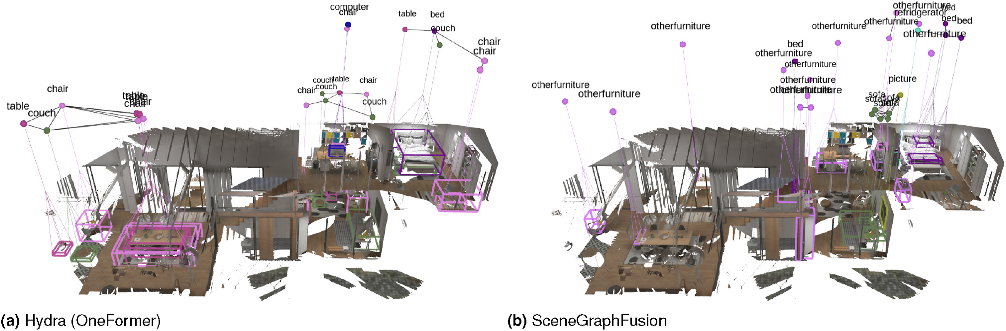

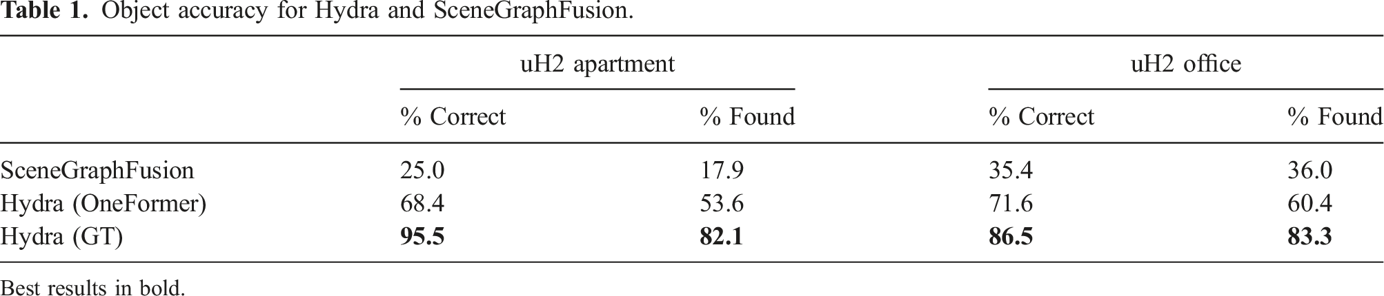
Table 1 shows that Hydra largely outperforms SceneGraphFusion in terms of both Percent Correct and Percent Found, even after disregarding the incorrect semantic labels for the objects produced by SceneGraphFusion. In hindsight, Hydra can benefit from more powerful 2D segmentation networks and estimate better objects, while SceneGraphFusion directly attempts to extract semantics from the 3D reconstruction, which is arguably a harder task and does not benefit from the large datasets available for 2D image segmentation. The last row in the table—Hydra (GT)—shows that Hydra’s accuracy can further improve with a better 2D semantic segmentation. While SceneGraphFusion is less competitive in terms of object understanding, we remark that it predicts a richer set of object relationships for each edge between objects (Wu et al., 2021) (e.g., standing on, attached to) compared to Hydra, which might be also useful for certain applications.

6.3.2. Accuracy evaluation and ablation

Here, we examine the accuracy of Hydra, running in real-time, as benchmarked against the accuracy attained by constructing a 3D scene graph in an offline manner (i.e., by running Kimera (Rosinol et al., 2021)). We also present a detailed quantitative analysis to justify key design choices in Hydra. To do this, we break down this quantitative analysis across the objects, places, and rooms layers. We examine the impact of (i) the choice of loop closure detection and 2D semantic segmentation on the accuracy of each layer of the 3D scene graph, and (ii) the impact of model architectures and training parameters on the accuracy of the room classification network. As such, we first present the accuracy of the predicted object and place layers by Hydra. We then move to looking at room classification accuracy, including two ablation studies on the neural tree and an evaluation of our room clustering approach based on persistent homology. Finally, we examine the quality of predicted loop closures when using the proposed hierarchical descriptors.

When benchmarking the accuracy of the layers of Hydra, we consider five different configurations for odometry estimation and loop closure detection. The first configuration (“GT-Trajectory”) uses ground-truth poses to incrementally construct the scene graph and disregards loop closures. The second, third, and fourth configurations (“VIO+V-LC,” “VIO+SG-LC,” and “VIO+GNN-LC,” respectively) use visual-inertial odometry (VIO) for odometry estimation and use vision-based loop closures (VIO+V-LC), the proposed hierarchical handcrafted descriptors for scene graph loop closures (VIO+SG-LC), or the proposed hierarchical learned descriptors for scene graph loop closures (VIO+GNN-LC). The last configuration, VIO, uses visual-inertial odometry without loop closures.

6.3.2.1. Accuracy evaluation: Objects

Figure 14 evaluates the object layer of Hydra across the five configurations of Hydra, as well as across various 2D semantic segmentation sources: ground-truth semantics (when available), OneFormer, HRNet, and MobileNetV2. For this evaluation, we benchmark against the ground-truth objects from the underlying Unity simulation for uHumans2. As the recording for the uHumans2 scenes only explores a portion of the scene, we only compare against ground-truth objects that have a high enough number of mesh vertices inside their bounding boxes (40 vertices). For the real datasets, where we do not have ground-truth objects, we consider the object layer of the batch scene graph constructed from ground-truth poses and OneFormer-based 2D semantic segmentation using Kimera (Rosinol et al., 2021) as the ground-truth objects for the purposes of evaluation. For the object layer, we report two metrics: the percentage of objects in the ground-truth scene graph that have an estimated object with the correct semantic label within a specified radius (“% Found”) and the percentage of objects in the estimated scene graph that have a ground-truth object with the correct semantic label within a specified radius (“% Correct”). ²²

Figure 14.

(a)–(e) Object accuracy metrics for all scenes across different 2D semantic segmentation sources and different LCD and pose source configurations. The metrics are averaged over 5 trials for each pair of configurations (i.e., there were 5 trials for every combination of 2D semantics and a pose source). For semantic segmentation sources, “OF” is Oneformer, “HR” is HRNet, “MN” is MobileNetV2, and “GT” is the ground truth semantic segmentation provided by the simulator. Each cell reports the mean and standard deviation. Values are colored from highest (dark green, best performance) to lowest (light yellow, worst performance) by mean. (f) Place layer accuracy for all scenes across different configurations for Hydra. Each bar shows the average distance error for a given scene and configuration over 5 trials; standard deviation across the 5 trials is shown as a black error bar.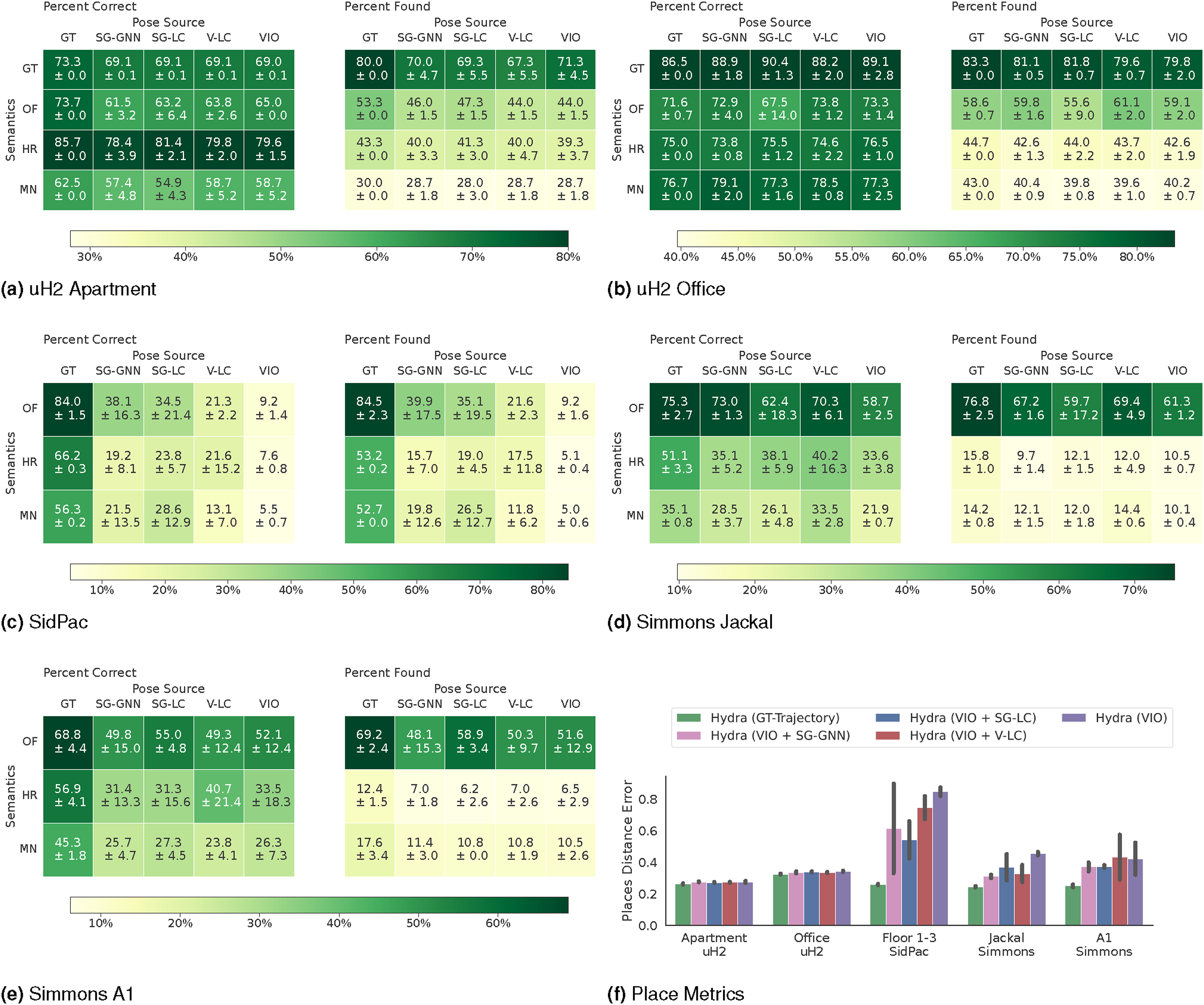

We note some important trends in Figure 14. First, when using GT-Trajectory, Hydra produces objects that are reasonably close to the ground-truth (80%–100% found and correct objects for the Office scene), or close to the objects produced by offline approaches (70%–80% found and correct objects for SidPac and Simmons). This demonstrates that—given the trajectory—the real-time scene graph from Hydra is comparable to the batch and offline approaches at the state of the art. Second, VIO+V-LC, VIO+SG-LC, and VIO+GNN-LC maintain reasonable levels of accuracy for the objects and attain comparable performance in small to medium-sized scenes (i.e., the uHumans2 Apartment, Office, and Simmons A1) for the same choice of semantic segmentation method. In these scenes, the drift is small and the loop closure strategy does not radically impact performance (differences are within standard deviation). However, in larger scenes (e.g., SidPac) scene graph loop closures are more important and both VIO+GNN-LC and VIO+SG-LC largely outperform VIO+V-LC and VIO in terms of object accuracy.

As expected, the quality of the semantic segmentation impacts the accuracy; this is much more pronounced for “% Found” than “% Correct.” We note that OneFormer counter-intuitively has a lower “% Correct” than HRNet for the uHumans2 scenes. One factor in this inversion in performance is that the two metrics are somewhat coupled; a lower “% Found” can lead to a higher “% Correct.” An additional factor responsible for the lower “% Correct” of Oneformer is that OneFormer is accurate enough to sometimes identify objects that exist in the scene that are not included in the ground-truth objects exported by the simulator. We also note a slight correlation between reduced semantic segmentation performance and reduced accuracy for VIO+GNN-LC and VIO+SG-LC, such as for the Simmons Jackal scene. The low number of objects identified by HRNet and MobileNetV2 in this scene contributes to fewer scene-graph based loop closures, and as such, worse performance.

Finally, we remark that even the GT-Trajectory configuration does not achieve 100% accuracy for “% Found” and “% Correct” for the uHumans2 scenes when using ground-truth semantics. Two main factors contribute to the imperfect performance of the GT-Trajectory configuration. The first is that the way Hydra extracts objects tends to under-segment nearby objects of the same class, leading to a predicted object centroid farther away from the individual ground truth object instances. The second is that the underlying metric-semantic reconstruction used in the active window (i.e., Kimera (Rosinol et al., 2020a) and Voxblox (Oleynikova et al., 2017)) occasionally results in object labels being projected to the surface behind objects, which leads to hallucinated objects.

6.3.2.2. Accuracy evaluation: Places

Figure 14(f) evaluates the place layer by comparing the five configurations for Hydra. We use either the ground-truth semantics (when available) or OneFormer (when ground-truth semantics is not available), as the places are not influenced by the semantic segmentation quality. For the places evaluation, we construct a “ground-truth” GVD from a 3D reconstruction of the entire scene using the ground-truth trajectory of the scene. Using this, we measure the mean distance of an estimated place node to the nearest voxel in the ground-truth GVD, which we call “Position Error.” Figure 14(f) reports this metric, along with standard deviation across 5 trials shown as black error bars.

We note some important trends in Figure 14(f). Similar to the case of objects, the place positions errors are almost identical for all configurations of Hydra for the uHumans2 scenes. These scenes have very low drift, and are relatively small, so it is expected that a higher quality trajectory makes less of an impact. For the larger scenes, we see a range of results. However, we see for SidPac, VIO+GNN-LC performs worse than VIO+SG-LC, though both outperform VIO+V-LC and VIO. Interestingly, we note that VIO+SG-LC performs slightly worse than VIO+V-LC for the Simmons Jackal scene, while VIO+GNN-LC does the same as VIO+V-LC (but with lower standard deviation, as indicated by the black confidence bars in the plot). Note that the Simmons Jackal scene has multiple uniform rooms with very similar objects and layouts. In general, VIO is outperformed by methods that incorporate loop closures, and the ability to correct for loop closures is important to maintaining an accurate 3D scene graph.

6.3.2.3. Neural tree ablation 1: Node classification

We first replicate the semi-supervised node classification experiment described in Talak et al. (2021) and compare different message passing architectures on the original graphs (i.e., standard GNNs) and on the H-tree (i.e., the proposed neural tree). To construct the H-tree graphs, we apply the proposed hierarchical tree decomposition algorithm (Algorithm 1), which concatenates the tree decomposition of each layer. The results are shown in Table 2 With the proposed tree decomposition approach, the neural tree achieves an advantage between 1.63% and 11.72% over standard GNN models, depending on the type of message passing architecture. In comparison to the results in Talak et al. (2021), the results in Table 2 are generated using a later version of the PyTorch Geometric library, which supports heterogeneous GNN operators. Also note that the tree decomposition used in Table 2 differs slightly from the tree decomposition algorithm used in Talak et al. (2021). We provide additional results in Appendix A.6 that examine the impact of these changes.

Table 2.

Stanford3d: Node classification accuracy for different message passing architectures.

Message passing	Original (%)	H-tree (%)
GCN	42.91 ± 2.01	54.63 ± 2.19
GraphSAGE	56.97 ± 2.02	58.60 ± 2.13
GAT	45.06 ± 2.32	53.71 ± 2.10
GIN	48.03 ± 2.21	55.00 ± 2.68

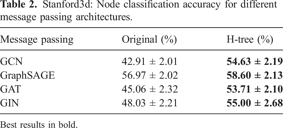
Best results in bold.

We note that the absolute position of a node centroid is not invariant to translation, and that invariance is important to generalize to new scenes regardless of the choice of coordinate frames. We therefore examine using the relative positions of node centroids as edge features, instead of including them directly as node features. For the H-tree, which contains clique nodes that are comprised of multiple objects or rooms, we use the mean room centroid as the centroid of the clique when computing relative positions. In addition, we also investigate the impact of using heterogeneous graphs (which can accommodate different node and edge types, as the ones arising in the 3D scene graph) against standard homogeneous graphs. For this comparison, we only use the GAT message passing function since it is the only one in Table 2 that can both handle heterogeneous message passing and incorporate edge features.

We present the results of this ablation study in Table 3. Comparing the two position encodings, the neural tree models achieve significantly higher accuracy when using relative positions as edge features: 7.45% on homogeneous graphs and 2.86% on heterogeneous graphs. Choosing features that are translation invariant (i.e., relative positions) has a clear advantage when using neural tree models. The standard GNNs show near-identical performance between the two position encodings. The heterogeneous graph structure has no significant impact on standard GNNs, but it degrades performance of the neural trees. The exact mechanism behind this decrease in performance in unclear; we posit that the heterogeneous neural tree variants have more parameters than the other architectures, and that the Standford3D dataset may not have enough training data for these architectures. We do not observe a significant performance decrease between the homogeneous and heterogeneous neural tree variants for the MP3D dataset.

Table 3.

Stanford3d: Node classification accuracy for different graph types and position encodings.

Graph types		Original (%)	H-tree (%)
Homogeneous	Absolute pos	45.06 ± 2.32	53.71 ± 2.10
	Relative pos	46.05 ± 1.98	61.16 ± 2.03
Heterogeneous	Absolute pos	46.56 ± 2.42	45.30 ± 2.57
	Relative pos	45.79 ± 2.04	48.16 ± 2.21

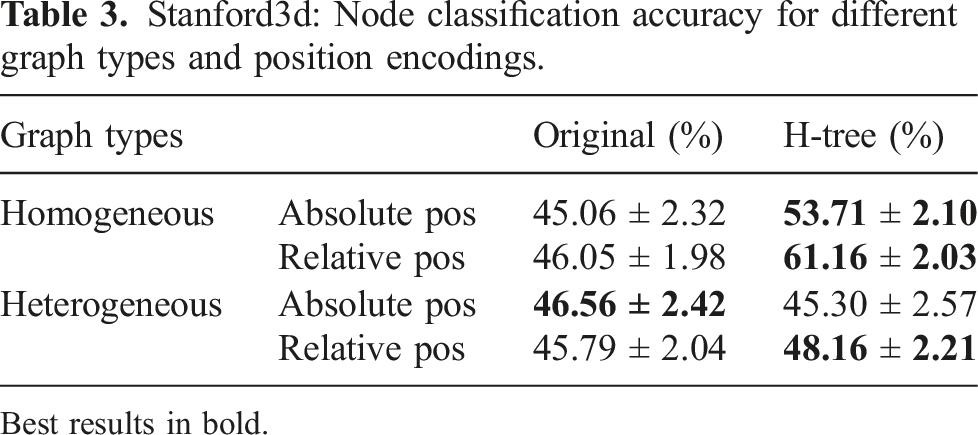
Best results in bold.

6.3.2.4. Neural tree ablation 2: Room classification

We compare the neural tree against standard GNNs on a room classification task using the MP3D dataset, predicting room semantic labels for the object-room graphs extracted from Hydra. Compared to Stanford3d, this dataset contains both semantic labels of the object nodes and room layer connectivity from Hydra, in addition to the geometric features (i.e., centroid position and bounding box size) of each node. Therefore, we study the effect of these two additional pieces of information. We use pre-trained word2vec vectors to represent object semantic labels and concatenate them with the geometric feature vectors. As described previously, we filter out partially explored rooms, using a threshold of 60% IoU. As before, we use GAT as the message passing function when training, as all graphs are heterogeneous and have edge features. The results are shown in Table 4. Both approaches show a significant performance improvement using the semantic labels of the objects, ranging from 14% to 17%. The neural tree also shows substantial improvement when incorporating room layer edges, while the standard GNNs do not. The best-performing neural tree model is obtained when using semantic labels for the objects and accounting for room connectivity; this is the model we use in the rest of this paper.

Table 4.

MP3D: Room classification accuracy for different graph types and node features.

Graph types		Original (%)	H-tree (%)
w/o word2vec	w/o room edges	41.28 ± 0.48	38.63 ± 0.25
	with room edges	41.20 ± 1.08	43.27 ± 0.59
with word2vec	w/o room edges	56.74 ± 0.85	55.84 ± 0.37
	with room edges	56.02 ± 0.84	57.67 ± 0.57

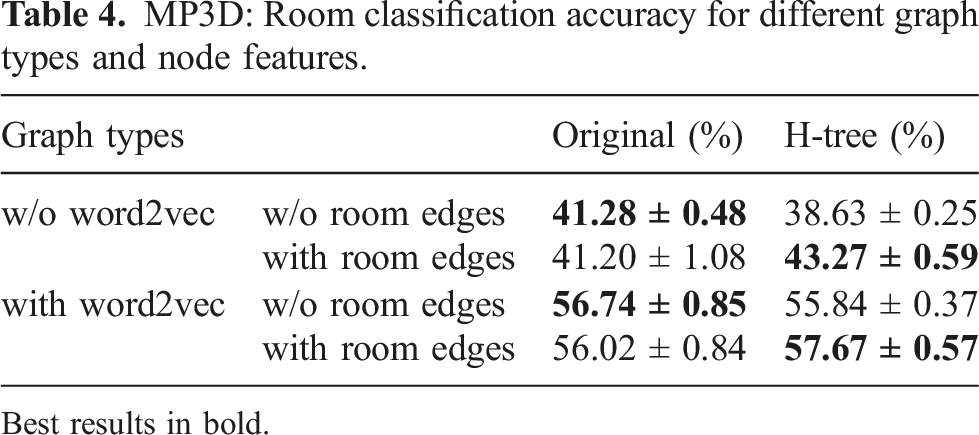
Best results in bold.

6.3.2.5. Accuracy evaluation: rooms

We evaluate the accuracy of the room segmentation in Hydra, by first evaluating the quality of the geometric room clustering described in Section 3.4.1 and then testing the room classification from Section 3.4.2 for different choices of 2D segmentation network.

Figure 15 evaluates the room clustering performance, using the precision and recall metrics defined in Bormann et al. (2016) (here we compute precision and recall over 3D voxels instead of 2D pixels). More formally, these metrics are:

$\begin{array}{ll}\mathit{Precision}& =\frac{1}{\left|{\mathit{R}}_{\mathit{e}}\right|}{\displaystyle \sum }_{{\mathit{r}}_{\mathit{e}}\in {\mathit{R}}_{\mathit{e}}}{\max }_{{\mathit{r}}_{\mathit{g}}\in {\mathit{R}}_{\mathit{g}}}\frac{\left|{\mathit{r}}_{\mathit{g}}\cap {\mathit{r}}_{\mathit{e}}\right|}{\left|{\mathit{r}}_{\mathit{e}}\right|}\\ \mathit{Recall}& =\frac{1}{\left|{\mathit{R}}_{\mathit{g}}\right|}{\displaystyle \sum }_{{\mathit{r}}_{\mathit{g}}\in {\mathit{R}}_{\mathit{g}}}{\max }_{{\mathit{r}}_{\mathit{e}}\in {\mathit{R}}_{\mathit{e}}}\frac{\left|{\mathit{r}}_{\mathit{e}}\cap {\mathit{r}}_{\mathit{g}}\right|}{\left|{\mathit{r}}_{\mathit{g}}\right|}\end{array}$

(12)

where R _e is the set of estimated rooms, R _g is the set of ground-truth rooms, and |⋅| returns the cardinality of a set; here, each room r _e (or r _g ) is defined as a set of free-space voxels. We hand-label the ground-truth rooms R _g from the ground-truth reconstruction of the environment. In particular, we manually define sets of bounding boxes for each room and then identify the set of free-space voxels for r _g as all free-space voxels that fall within any of the defined bounding boxes for r _g . For the estimated rooms R _e , we derive the set of free-space voxels r _e from the places comprising each estimated room. In equation (12), Precision then measures the maximum overlap in voxels with a ground-truth room for every estimated room, and Recall measures the maximum overlap in voxels with an estimated room for every ground-truth room. Intuitively, low precision corresponds to under-segmentation, i.e., fewer and larger room estimates, and low recall corresponds to over-segmentation, i.e., more and smaller room estimates. For benchmarking purposes, we also include the approach in Rosinol et al. (2021) (Kimera) as a baseline for evaluation.

Figure 15.

Room metrics for all scenes across different LCD pose source configurations. Each bar shows the average precision or recall over 5 trials; standard deviation across the 5 trials is shown as a black error bar.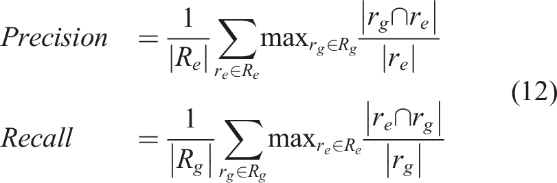

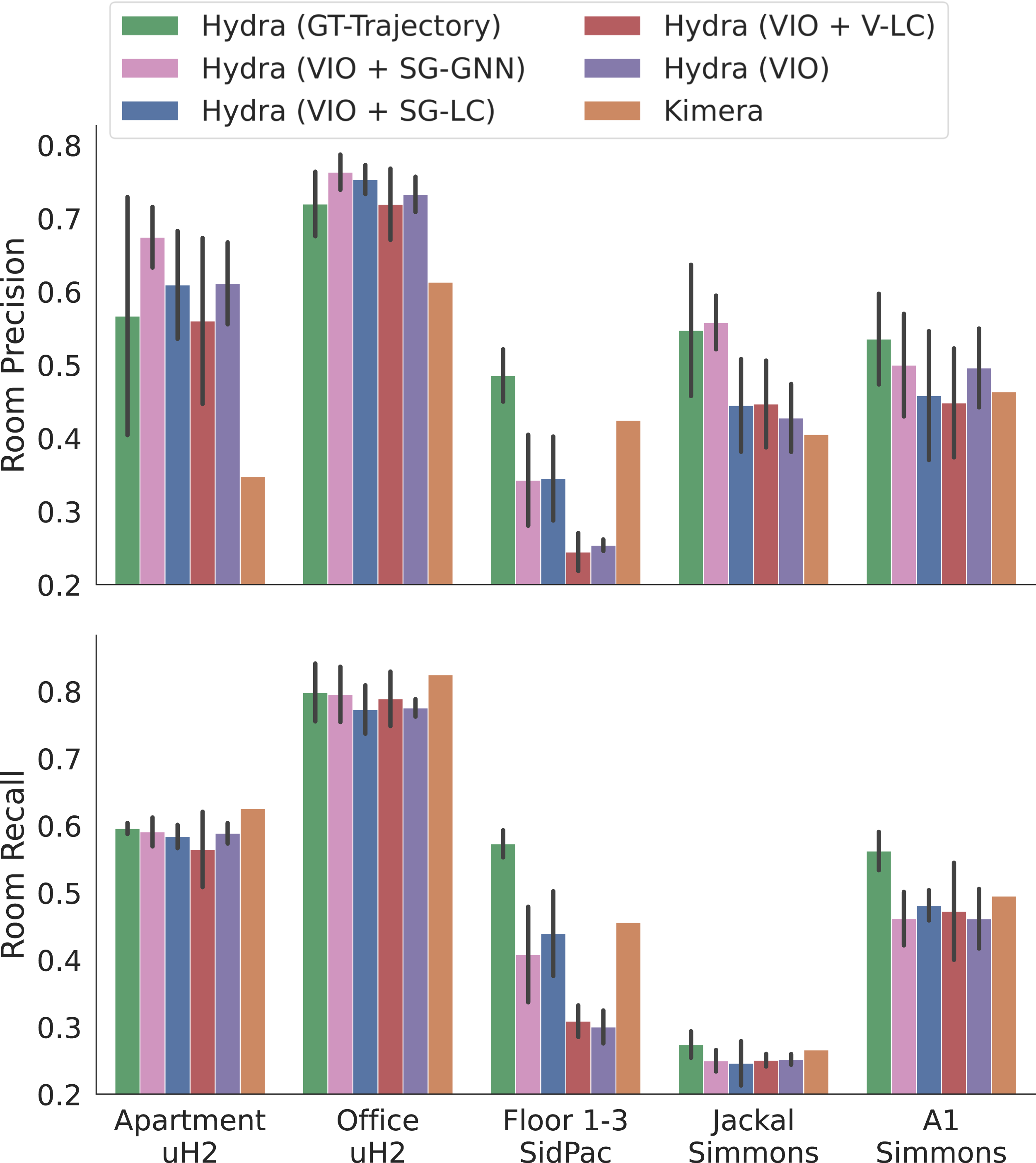
Figure 15 shows that Hydra generally outperforms Kimera (Rosinol et al., 2021) when given the ground-truth trajectory, and that Hydra is slightly more robust to multi-floor environments. This is expected, as Kimera performs room segmentation by taking a 2D slice of the voxel-based map of the environment, which does not generalize to multi-floor scenes. For both the split-level Apartment scene and the multi-floor SidPac scene, we achieve higher precision as compared to Kimera. These differences stem from the difficulty of setting an appropriate height to attempt to segment rooms at for Kimera (this is the height at which Kimera takes a 2D slice of the ESDF). Finally, it is worth noting that our room segmentation approach is able to mostly maintain the same levels of precision and recall for VIO+GNN-LC, VIO+SG-LC and VIO+V-LC. In some cases, our approach outperforms Kimera, despite the drift inherent in VIO+GNN-LC, VIO+SG-LC and VIO+V-LC (Kimera uses ground-truth poses).

Finally, we report room classification accuracy for uHumans2, SidPac, and Simmons across semantic segmentation sources in Table 5 using the proposed neural tree. We manually assign a ground-truth room category to each hand labeled ground-truth room, and compute the percentage of estimated room labels that match their corresponding ground-truth category. Label correspondences are computed by picking the ground-truth room that contains the most place nodes that comprise each estimated room; an estimated room is assigned a correspondence to unknown if too few place nodes (less than 10) fall inside the best ground-truth room.

Table 5.

Room classification accuracy for Hydra.

	GT	HRNet (%)	OneFormer (%)
uHumans2 Apartment	26.7 ± 3.7%	38.0 ± 21.7	45.0 ± 11.2
uHumans2 Office	27.6 ± 7.5%	28.4 ± 6.9	27.0 ± 10.1
SidPac Floor 1–3	N/A	46.2 ± 11.9	47.7 ± 12.5
Simmons Jackal	N/A	32.3 ± 16.6	15.3 ± 6.5
Simmons A1	N/A	29.0 ± 24.4	38.0 ± 28.0

We note two interesting trends. First, the richness of the object label space impacts the predicted room label accuracy, as shown by the relatively poor performance of the GT column as compared to either HRNet or OneFormer for the uHumans2 scenes (27% versus 40% or 45%): the GT semantics available in the simulator has a smaller number of semantic classes for the objects, hindering performance. This is consistent with the observations in Chen et al. (2022). Second, scenes such as the uHumans2 office or Simmons that are out of distribution—compared to the MP3D dataset we use for training—perform poorly. An example of a resulting 3D scene graph for SidPac with room category labels is shown in Figure 1.

6.3.2.6. Loop closure ablation

Finally, we take a closer look at the quality of the loop closures candidates proposed by our hierarchical loop closure detection approach, and compare it against traditional vision-based approaches on the Office scene. In particular, we compare our approach against a vision-based loop closure detection that uses DBoW2 for place recognition and ORB feature matching, as described in Rosinol et al. (2021).

Figure 16 shows the number of detected loop closures against the error of the registered solution (i.e., the relative pose between query and match computed by the geometric verification) for four different loop closure configurations: (i) “SG-LC”: the proposed handcrafted scene graph loop closure detection, (ii) “SG-GNN”: the proposed learned scene graph loop closure detection, (iii) “V-LC (Nominal)”: a traditional vision-based loop closure detection with nominal parameters, and (iv) “V-LC (Permissive)”: a vision-based loop closure detection with more permissive parameters (i.e., a decreased score threshold and less restrictive geometric verification settings). We report key parameters used in this evaluation in Appendix A.7. As expected, making the vision-based detection parameters more permissive leads to more but lower-quality loop closures. On the other hand, the scene graph loop closure approach produces approximately twice as many loop closures within 10 cm of translation error and 1° of rotation error as the permissive vision-based approach. The proposed approach produces quantitatively and quantitatively better loop closures compared to both baselines. Notably, SG-GNN also outperforms both vision baselines and the SG-LC. We present further discussion and a breakdown of additional statistics of the proposed loop closures of each method in Appendix A.8.

Figure 16.

Number of detected loop closures versus error of the estimated loop closure pose for four different loop closure detection configurations. Five individual trials and a trend-line are shown for each configuration.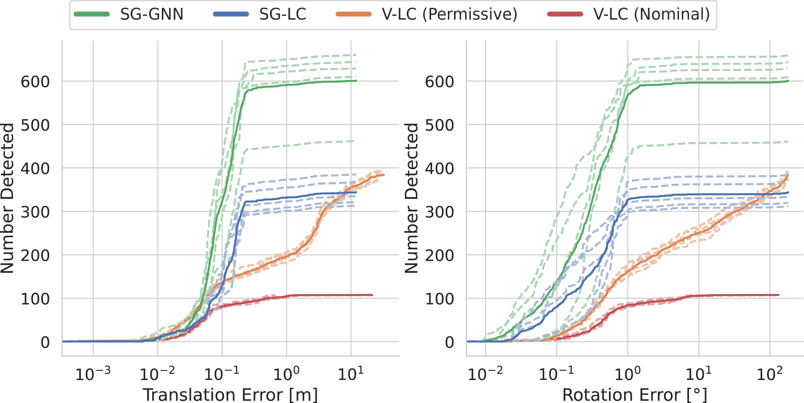

To further examine the relative performance of SG-LC and SG-GNN, we evaluate the top-k precision of both approaches on both the test split of the MP3D dataset used to train the descriptors, and the uHumans2 office scene. For this metric, we compute the percent of the k-highest-scored ²³ descriptors for each query descriptor that are valid matches; two descriptors are determined to match if the bounding box of their corresponding sub-graphs have a IoU above a specified threshold. We include two configurations of SG-GNN for object sub-graphs in this analysis; one that uses a one-hot encoding and one that uses word2vec embeddings to represent the semantic labels of the object nodes. We report this metric for both SG-LC (handcrafted) and SG-GNN (learned) in Table 6 for two IoU thresholds: 0.4 and 0.6.

Table 6.

p@k results for loop closure detection.

			p@10
			IoU = 0.4	IoU = 0.6
Objects	MP3D	Handcrafted	70.9	58.6
		Learned + OneHot	65.5	56.0
		Learned + Word2Vec	60.3	50.9
	uH2 Office	Handcrafted	46.5	31.5
		Learned + OneHot	47.4	31.4
		Learned + Word2Vec	37.6	26.5
Places	MP3D	Handcrafted	76.4	58.0
		Learned	59.5	47.4
	uH2 Office	Handcrafted	68.6	41.4
		Learned	54.1	34.9

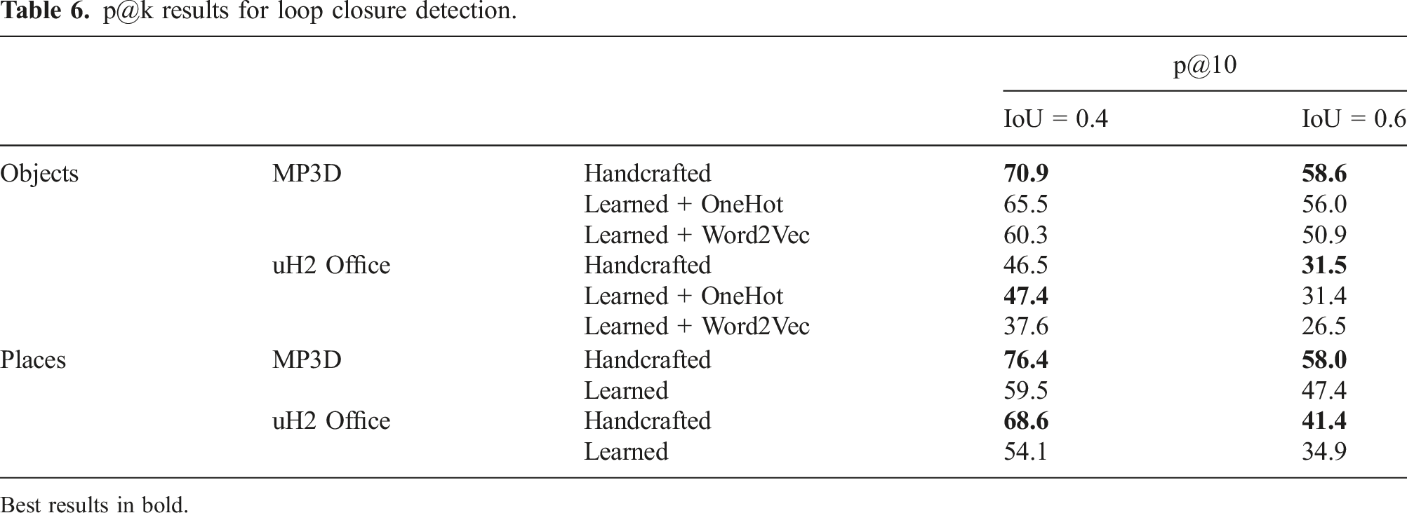
Best results in bold.

We note some interesting trends in Table 6. First, the one-hot encoding outperforms the word2vec encoding for both datasets, and appears to transfer better between datasets (i.e., showing 5% better performance for the MP3D dataset, but 10% better performance for uHumans2). Additionally, the original handcrafted descriptors maintain good performance compared to the learned descriptors, and only the learned object descriptors appear competitive to the handcrafted descriptors in terms of precision. We believe that the high performance of the handcrafted descriptors is due to the semantic and geometric diversity among the scenes of the MP3D dataset. Previous experiments (using the VIO+GNN-LC configuration of Hydra) imply that the learned descriptors offer improved performance in environments with a more uniform object distribution (i.e., the Simmons Jackal scene).

6.3.3. Onboard operation on a robot

This section shows that Hydra is capable of running in real-time and is deployable to a robot. We show this by performing a qualitative experiment, running Hydra online on the Unitree A1. We run Hydra and the chosen 2D semantic segmentation network (MobilenetV2 (Sandler et al., 2018)) on the Nvidia Xavier NX mounted on the back of the A1. Additionally, we run our room classification approach in the loop with Hydra on the CPU of the same Nvidia Xavier. In this test, to circumvent the computational cost of running Kimera-VIO, we use an Intel RealSense T265 to provide odometry estimates to Hydra. As a result, we use our proposed scene-graph loop closure detection method without the appearance-based descriptors (which would rely on Kimera-VIO for computation of the visual descriptors and vision-based geometric verification). To maintain real-time performance, we configure the frontend of Hydra to run every fifth keyframe (instead of every keyframe), and limit the reconstruction range to 3.5 m (instead of the nominal 4.5 m). Note that this results in a nominal update rate of 1 Hz for Hydra, though we still perform dense 3D metric-semantic reconstruction at keyframe rate (5 Hz). A breakdown of the runtime of Hydra’s modules during this experiment is available in Section 6.3.4.

For this experiment, we partially explore a floor of building 31 on the MIT campus consisting of a group of cubicles, a conference room, two impromptu lounge areas, all of which are connected by a hallway. An intermediate scene graph produced by Hydra while running the experiment is shown in Figure 17, and the experiment itself is shown in the video supplement.

Figure 17.

Intermediate 3D scene graph created by Hydra onboard the A1 quadruped while exploring building 31 on the MIT campus. Estimated room labels are shown. The entire mapping sequence is shown in the video supplement.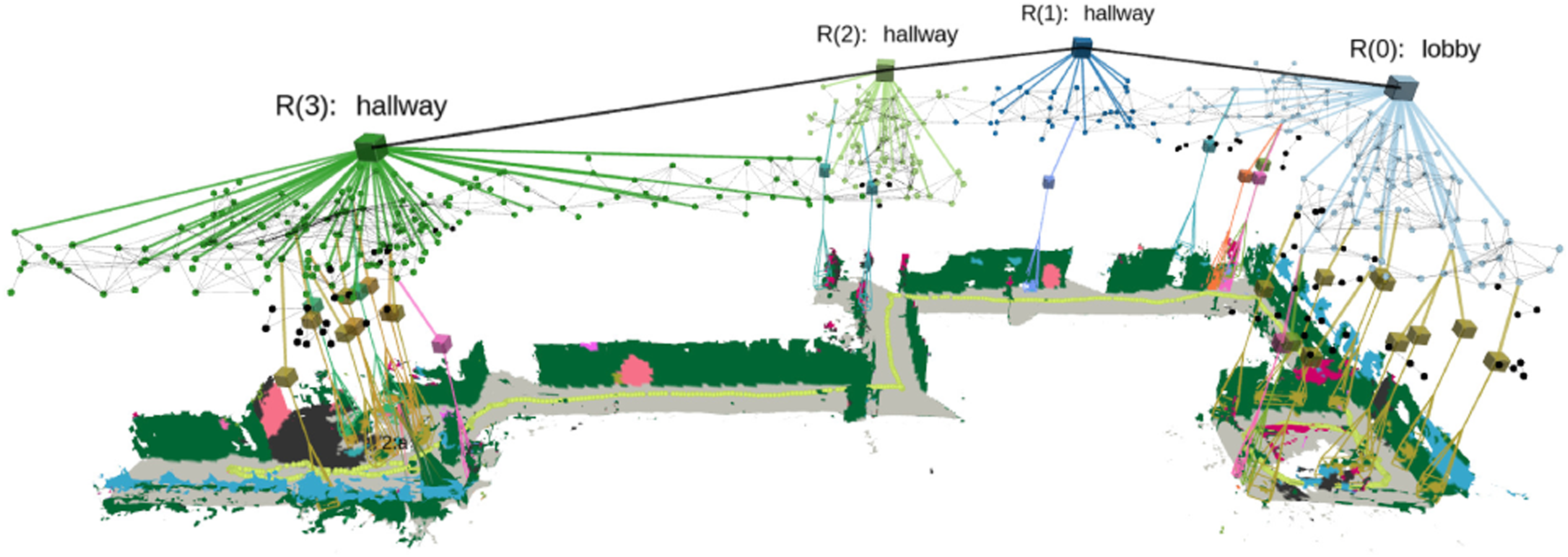

Hydra estimates four rooms for the scene graph; of these four rooms, room 3 is centered over one of the two lounges, and room 0 covers both the conference room (located in the lower right corner of Figure 17) and a portion of the hallway. Qualitatively, Hydra over-segments the scene, but the produced rooms and labels are still somewhat consistent with the underlying room structure and labels. In this instance, only room 0 has an incorrectly estimated label; however the room categories that Hydra estimates over the course of the experiment are not as consistent. This is likely due to the poor quality of the 2D semantics from MobilenetV2, and general lack of useful object categories for inferring room labels.

6.3.4. Runtime evaluation

Figure 18 reports the runtime of Hydra versus the batch approach in Rosinol et al. (2021). This plot shows that the runtime of the batch approach increases over time and takes more than 5 minutes to generate the entire scene graph for moderate scene sizes; as we mentioned, most processes in the batch approach (Rosinol et al., 2021) entail processing the entire ESDF (e.g., place extraction and room detection), inducing a linear increase in the runtime as the ESDF grows. On the other hand, our scene graph frontend (Hydra Mid-Level in Figure 18) has a fixed computation cost. In Figure 18, a slight upward trend is observable for Hydra High-Level, driven by room detection and scene graph optimization computation costs, though remaining much lower than batch processing. Noticeable spikes in the runtime for Hydra High-Level (e.g., at 1400 s) correspond to the execution of the 3D scene graph optimization when new loop closures are added.

Figure 18.

Runtime required for scene graph construction vs. timestamp for the SidPac Floor 1–3 dataset for a batch approach (Kimera) and for the proposed incremental approach (Hydra). The middle subplot shows runtime information from the same experiment as the top, but zoomed in to highlight the behavior of Hydra High-Level. The bottom subplot shows runtime information from the same experiment as the first but zoomed in to highlight the behavior of Hydra Mid-Level. We filter out measurements of Hydra High-Level less than 20 ms to clarify trends in the bottom subplot. For timing of the low-level processes in Hydra, we refer the reader to the analysis in Rosinol et al. (2021), as we also rely on Kimera-VIO.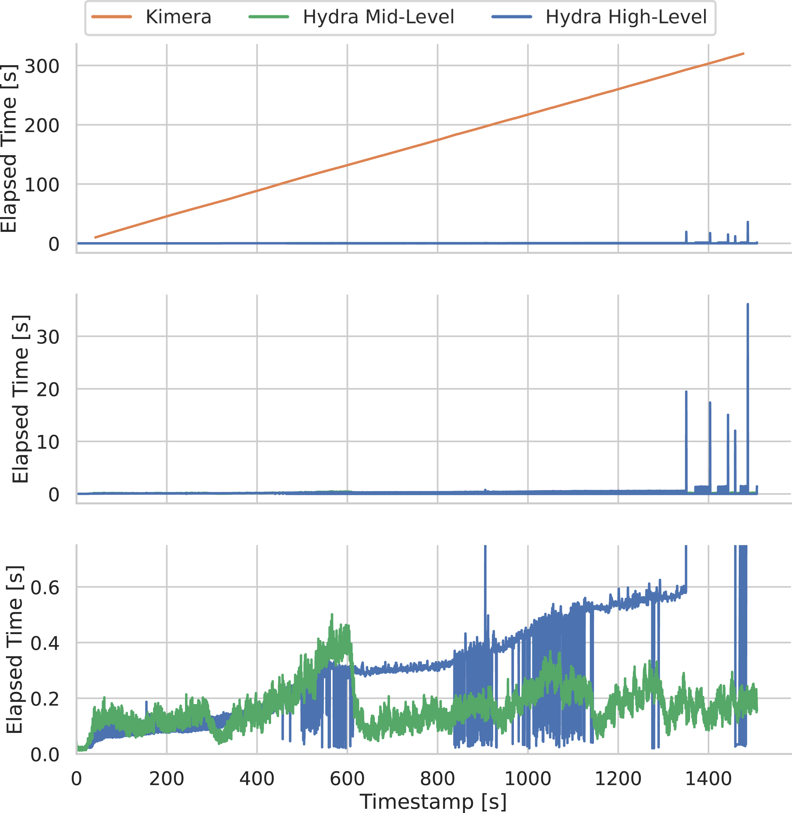

When reconstructing the scene shown in Figure 18 (SidPac Floor1–3), Hydra uses a maximum of 7.2 MiB for the TSDF, 19.1 MiB for the storage of the semantic labels, and 47.8 MiB for the storage of the dense GVD inside the active window, for a total of 74.1 MiB. Kimera instead uses 79.2 MiB for the TSDF, 211 MiB for the storage of semantic labels, and 132 MiB for the storage of the ESDF when reconstructing the entire environment, for a total of 422 MiB of memory. Note that the memory storage requirement of Hydra for the active window is a fifth of the memory required for Kimera, and that the memory usage of Kimera grows with the size of the scene.

Table 7 reports timing breakdown for the incremental creation of each layer across scenes for a single trial. The object layer runtime is determined by the number of mesh vertices in the active window and the number of possible object semantic classes. The room layer runtime is determined by the number of places (a combination of how complicated and large the scene is); this is why the Office has the largest computation cost for the rooms despite being smaller than the SidPac scenes. Note that our target keyframe rate implies a limit of 200 ms for any of these processes. While the mean and standard deviation of all layers are well below this rate, we do see that the real-time rate is exceeded in some cases for extracting the objects. This specifically occurs for larger scenes (i.e., SidPac and Simmons Jackal), due to the presence of many objects. At the same time, we remark that Hydra is architected in such a way that temporarily exceeding the real-time threshold does not preclude online performance and real-time operation is restored shortly after these delays occur.

Table 7.

Hydra: Timing breakdown.

	Objects (ms)	Places (ms)	Rooms (ms)
uH2 Apartment	52.8 ± 14.9	11.3 ± 6.1	1.8 ± 0.9
uH2 Office	34.0 ± 26.1	12.5 ± 6.9	14.6 ± 11.9
SidPac Floor 1–3	57.4 ± 55.7	15.7 ± 9.2	5.9 ± 9.0
Simmons Jackal	63.9 ± 45.8	19.6 ± 13.1	6.6 ± 9.0
Simmons A1	71.1 ± 50.5	18.6 ± 11.7	1.4 ± 1.0

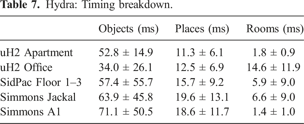
While the timing results in Table 7 are obtained with a relatively powerful workstation, here we restate that Hydra can run in real-time on embedded computers commonly used in robotics applications. Towards this goal, we report the timing statistics from the online experiment running Hydra onboard the Unitree A1 as shown in Figure 17. Hydra processes the objects in 83.9 ± 65 ms, places in 114.8 ± 103 ms, and rooms in 34.7 ± 37.6 ms. While these numbers imply that Hydra can run faster than the 1 Hz target rate on the Xavier, we note that the 1 Hz limit is chosen to not fully max out the computational resources of the Xavier. Additionally, there are other modules of Hydra and external processes that limit (sometimes significantly) the computational resources of the Xavier (e.g., the reconstruction of the TSDF and GVD). While there is still margin to optimize computation (see conclusions), these initial results stress the practicality and real-time capability of Hydra in building 3D scene graphs.

7. Related work

We provide a broad literature review touching on abstractions and symbolic representations (Section 7.1), metric-semantic and hierarchical map representations and algorithms to build them from sensor data (Section 7.2), and loop closure detection and optimization (Section 7.3).

7.1. Need for abstractions and symbolic representations

7.1.1. State and action abstractions

The need to abstract sensor data into higher-level representations has been studied in the context of planning and decision-making. Konidaris (2019) points out the necessity of state and action abstraction for efficient task and motion planning problems. Konidaris et al. (2018) extract task-specific state abstractions. James et al. (2020) show how task-independent state abstractions can also be learned. James et al. (2022) show how to autonomously learn object-centric representations of a continuous and high-dimensional environment, and argue that such a representation enables efficient planning for long-horizon tasks. Berg et al. (2022) propose a hierarchical representation for planning in large outdoor environments. The hierarchy contains three levels: landmarks (e.g., forests, buildings, streets), neighborhoods, and cities. Several related works also discuss action abstractions, e.g., how to group a sequence of actions into macro-actions (usually referred to as options). Jinnai et al. (2019), for instance, provide a polynomial-time approximation algorithm for learning options for a Markov decision process.

7.1.2. Ontologies and knowledge graphs

A fundamental requirement for an embodied agent to build and communicate a meaningful representation of an environment is to use a common vocabulary describing concepts of interest ²⁴ and their relations. Such a vocabulary may be represented as an ontology or knowledge graph. The precise definition of an ontology varies between communities (Guarino et al., 2009; Jepsen 2009). A well accepted definition was proposed by Gruber (1995) as an explicit specification of conceptualization and later extended to require the conceptualization must be a shared view (Borst 1997) and written as a formal language (Studer et al., 1998). In practice, the definition used is often not as strict. For example, the definition provided by W3C as part of the Web Ontology Language (OWL) (McGuinness and Van Harmelen 2004) describes an ontology as a set of terms in a vocabulary and their inter-relationships. Generally, an embodied agent is committed to a conceptualization regardless if the commitment is explicit (e.g., represented as knowledge graph) or implicit (e.g., represented as a set of labels for a classifier) (Genesereth and Nilsson 2012).

The need to create a standard ontology was identified by Schlenoff et al. (2012), which resulted in the emergence of several knowledge processing frameworks focused on robotics applications (Beetz et al., 2018; Diab et al., 2019; Lemaignan et al., 2010; Tenorth and Beetz 2013). A significant effort has been made in the creation of common-sense ontologies and knowledge graphs (Auer et al., 2007; Bollacker et al., 2008; Carlson et al., 2010; Lenat 1995; Miller 1995; Niles and Pease 2001; Speer et al., 2017; Suchanek et al., 2008; Vrandečić and Krötzsch 2014). In recent years, there has been a surge in applying these ontologies and knowledge graphs to problems such as 2D scene graph generation (Amodeo et al., 2022; Chen et al., 2023; Guo et al., 2021; Zareian et al., 2020), image classification (Movshovitz-Attias et al., 2015; Porello et al., 2015), visual question answering (Aditya et al., 2018; Ding et al., 2022; Gardères et al., 2020; Marino et al., 2021; Zheng et al., 2021), task planning Chen et al. (2020); Daruna et al. (2021); Tuli et al. (2022), and representation learning (Hao et al., 2019; Kwak et al., 2022), to name a few.

7.1.3. Scene grammars and compositional models

Compositionality, which is the ability of humans to perceive reality as a hierarchy of parts, has been considered fundamental to human cognition (Geman et al., 2002; Lake et al., 2017). Geman et al. (2002) propose a mathematical formulation of compositional models, by recursively grouping or composing constituents and assigning probability factors to composition. Zhu et al. (2011) represent and infer visual patters as a recursive compositional model, which is nothing but a tree-structured graphical model where the leaf nodes represent the visual patters, and the higher-layers represent complex compositions. Zhu and Mumford (2006); Zhu and Huang (2021) discuss how to model objects, images, and scenes using such a hierarchical tree structure, called stochastic grammar, and advocate it to be a general framework for visual representation. Inspired by these insights, recent works such as Izatt and Tedrake (2020); Qi et al. (2018); Chua (2018) propose probabilistic generative models to capture hierarchical relationship between entities in a scene.

Recent works have tended to use such a hierarchical structure along with deep neural networks to provide better learning models. Wang et al. (2022) show that using a hierarchical, compositional model of the human body results in better human pose estimation. The model consists of body parts (e.g., shoulder, elbow, arm) organized as a hierarchy (e.g., shoulder, elbow are children of arm). A bottom-up/top-down inference strategy is proposed that is able to correct ambiguities in perceiving the lowest-level parts. Niemeyer and Geiger (2021) show that modeling a 3D scene as one composed of objects and background leads to more controllable and accurate image synthesis. Mo et al. (2020) model object shape as a hierarchical assembly of individual parts, and the object shape is then generated by transforming the shape parameter of each object part. Ichien et al. (2021) show that compositional model significantly outperform deep learning models on the task of analogical reasoning. Yuan et al. (2023) survey work on compositional scene representation. While early work by Fodor and Pylyshyn (1988) argued that neural-network-based models are not compositional in nature, recent works have suggested otherwise. The works (Mhaskar 1996; Mhaskar and Poggio 2016; Poggio et al., 2017) show that deep convolutional networks avoid the curse of dimensionality in approximating a class of compositional functions. Webb et al. (2022) show that large language models such as GPT-3 show compositional generalizability as an emergent property. Such compositionality, however, is not yet evident in generative models trained on multi-object scenes (Xie et al., 2022).

7.2. Metric-semantic and hierarchical representations for scene understanding and mapping

7.2.1. 2D scene graphs in computer vision

2D scene graphs are a popular model for image understanding that describes the content of an image in terms of objects (typically grounded by bounding boxes in the image) and their attributes and relations (Johnson et al., 2015; Krishna et al., 2016). The estimation of 2D scene graphs (either from a single image or a sequence of images) has been well studied in the computer vision community and is surveyed in Zhu et al. (2022). The seminal works (Johnson et al., 2015; Krishna et al., 2016) advocated the use of 2D scene graphs to perform cognitive tasks such as image search, image captioning, and answering questions. These tasks, unlike object detection, require the model to reason about object attributes and object-to-object relations, and therefore, enable better image understanding. 2D scene graphs have been successfully used in image retrieval (Johnson et al., 2015), caption generation (Anderson et al., 2016; Karpathy and Fei-Fei 2015), visual question answering (Krishna et al., 2016; Ren et al., 2015), and relationship detection (Lu et al., 2016). GNNs are a popular tool for joint object labels and/or relationship inference on scene graphs (Li et al., 2017; Xu et al., 2017; Yang et al., 2018; Zellers et al., 2017). Chang et al. (2023a) provide a comprehensive survey on the various methods that have been proposed to infer a 2D scene graph from an image.

Despite their popularity, 2D scene graphs have several limitations. First of all, they are designed to ground concepts in the image space, hence they are not suitable to model large-scale scenes (see discussion in Section 2). Second, many of the annotated object-to-object relationships in Krishna et al. (2016) like “behind,” “next to,” “near,” “above,” and “under” are harder to assess from a 2D image due to the lack of depth information, and are more easily inferred in 3D. Finally, 2D representations such as 2D scene graphs are not invariant to viewpoint changes (i.e., viewing the same 3D scene from a different viewing angle may result in a different 2D scene graph), as observed in Armeni et al. (2019).

7.2.2. Flat metric-semantic representations

The last few years have seen a surge of interest towards metric-semantic mapping, simultaneously triggered by the maturity of traditional 3D reconstruction and SLAM techniques, and by the novel opportunities for semantic understanding afforded by deep learning. The literature has focused on both object-based maps (Bowman et al., 2017; Dong et al., 2017; Nicholson et al., 2018; Ok et al., 2021; Salas-Moreno et al., 2013; Shan et al., 2020) and dense maps, including volumetric models (Grinvald et al., 2019; McCormac et al., 2017; Narita et al., 2019), point clouds (Behley et al., 2019; Lianos et al., 2018; Tateno et al., 2015), and 3D meshes (Rosinol et al., 2020a; Rosu et al., 2019). Some approaches combine objects and dense map models (Li et al., 2016; McCormac et al., 2018; Schmid et al., 2021; Xu et al., 2019a). These approaches are not concerned with estimating higher-level semantics (e.g., rooms) and typically return dense models that might not be directly amenable for navigation (Oleynikova et al., 2018).

7.2.3. Building parsing

A somewhat parallel research line investigates how to parse the layout of a building from 2D or 3D data. A large body of work focuses on parsing 2D maps (Bormann et al., 2016), including rule-based (Kleiner et al., 2017) and learning-based methods (Liu et al., 2018). Friedman et al. (2007) compute a Voronoi graph from a 2D occupancy grid, which is then labeled using a conditional random field. Recent work focuses on 3D data. Liu et al. (2018) and Stekovic et al. (2021) project 3D point clouds to 2D maps, which however is not directly applicable to multi-story buildings. Furukawa et al. (2009) reconstruct floor plans from images using multi-view stereo combined with a Manhattan World assumption. Lukierski et al. (2017) use dense stereo from an omni-directional camera to fit cuboids to objects and rooms. Zheng et al. (2020) detect rooms by performing region growing on a 3D metric-semantic model.

7.2.4. Hierarchical representations and 3D scene graphs

Hierarchical maps have been pervasive in robotics since its inception (Chatila and Laumond 1985; Kuipers 1978, 2000; Thrun 2003). Early work focuses on 2D maps and investigates the use of hierarchical maps to resolve the divide between metric and topological representations (Beeson et al., 2010; Choset and Nagatani 2001; Galindo et al., 2005; Ruiz-Sarmiento et al., 2017; Zender et al., 2008). These works preceded the “deep learning revolution” and could not leverage the rich semantics currently accessible via deep neural networks.

More recently, 3D scene graphs have been proposed as expressive hierarchical models for 3D environments. Armeni et al. (2019) model the environment as a graph including low-level geometry (i.e., a metric-semantic mesh), objects, rooms, and camera locations. Rosinol et al. (2021, 2020b) augment the model with a topological map of places (modeling traversability), as well as a layer describing dynamic entities in the environment. The approaches in Armeni et al. (2019); Rosinol et al. (2021, 2020b) are designed for offline use. Other papers focus on reconstructing a graph of objects and their relations (Kim et al., 2019; Wald et al., 2020; Wu et al., 2021). Wu et al. (2021) predict objects and relations in real-time using a graph neural network. Izatt and Tedrake (2021) parse objects and relations into a scene grammar model using mixed-integer programming. Gothoskar et al. (2021) use an MCMC approach. Gay et al. (2018) use a quadric representation to estimate 3D ellipsoids for objects in the scene given input 2D bounding boxes, and use an RNN to infer relationships between detected objects.

7.3. Maintaining persistent representations

7.3.1. Loop closures detection

Established approaches for visual loop closure detection in robotics trace back to place recognition and image retrieval techniques in computer vision; these approaches are broadly adopted in SLAM pipelines but are known to suffer from appearance and viewpoint changes (Lowry et al., 2016). Alternative approaches investigate place recognition using image sequences (Garg and Milford 2021; Milford and Wyeth 2012; Schubert et al., 2021) or deep learning (Arandjelovic et al., 2016). More related to our proposal is the set of papers leveraging semantic information for loop closure detection. Gawel et al. (2018) perform object-graph-based loop closure detection using random-walk descriptors built from 2D images. Liu et al. (2019) use similar object-based descriptors but built from a 3D reconstruction. Lin et al. (2021) adopt random-walk object-based descriptors and then compute loop closure poses via object registration. Qin et al. (2021) propose an object-based approach based on sub-graph similarity matching. Zheng et al. (2020) propose a room-level loop closure detector. None of these approaches are hierarchical in nature.

7.3.2. Loop closures correction

After a loop closure is detected, the map needs to be corrected accordingly. While this process is easy in sparse (e.g., landmark-based) representations (Cadena et al., 2016), it is non-trivial to perform in real-time when using dense representations. Stückler and Behnke (2014) and Whelan et al. (2016) optimize a map of surfels, to circumvent the need to correct structured representations (e.g., meshes or voxels). Dai et al. (2017) propose reintegrating a volumetric map after each loop closure. Reijgwart et al. (2020) correct drift in volumetric representations by breaking the map into submaps that can be rigidly re-aligned after loop closures. Whelan et al. (2015) propose a 2-step optimization that first corrects the robot trajectory and then deforms the map (represented as a point cloud or a mesh) using a deformation graph approach (Sumner et al., 2007). Rosinol et al. (2021) unify the two steps into a single pose graph and mesh optimization. None of these works are concerned with simultaneously correcting multiple layers in a hierarchical representation.

8. Conclusions

This paper argues that large-scale spatial perception for robotics requires hierarchical representations. In particular, we show that hierarchical representations scale better in terms of memory and are more suitable for efficient inference. Our second contribution is to introduce algorithms to build a hierarchical representation of an indoor environment, namely a 3D scene graph, in real-time as the robot explores the environment. Our algorithms combine 3D geometry (e.g., to cluster the free space into a graph of places), topology (to cluster the places into rooms), and geometric deep learning (e.g., to classify the type of rooms the robot is moving across). Our third contribution is to discuss loop closure detection and correction in 3D scene graphs. We introduce (handcrafted and learning-based) hierarchical descriptors for loop closure detection, and develop a unified optimization framework to correct drift in the 3D scene graph in response to loop closures. We integrate our algorithmic contributions into a heavily parallelized system, named Hydra, and show it can build accurate 3D scene graphs in real-time across a variety of photo-realistic simulations and real datasets.

8.1. Limitations

While we believe the proposed contributions constitute a substantial step towards high-level scene understanding and spatial perception for robotics, our current proposal has several limitations. First, the sub-graph of places captures the free-space in 3D, which is directly usable for a drone to navigate. However, traversability for ground robots is also influenced by other aspects (e.g., terrain type, steepness). These aspects are currently disregarded in the construction of the GVD and the places sub-graph, but we believe they are particularly important for outdoor extensions of 3D scene graphs. Second, our approach for room segmentation, which first clusters the rooms geometrically, and then labels each room, mainly applies to rooms with clear geometric boundaries (e.g., it would not work in an open floor-plan). We believe this limitation is surmountable (at the expense of using extra training data) by replacing the 2-stage approach with a single learning-based method (e.g., a neural tree or a standard graph neural network) that can directly classify places into rooms. Third, for computational reasons, we restricted the inference in the neural tree to operate at the level of objects, rooms, and buildings. However, it would be desirable for high-level semantic concepts (e.g., room and object labels) to propagate information downward towards the mesh geometry. While a more compact representation of the low-level geometry (Czarnowski et al., 2020; Sucar et al., 2020) might facilitate this process, it remains unclear how to fully integrate top-down reasoning in the construction of the 3D scene graph, which is currently a bottom-up process.

8.2. Future work

This work opens many avenues for current and future investigation. First of all, while this paper mostly focused on inclusion and adjacency relations, it would be interesting to label nodes and edges of the 3D scene graph with a richer set of relations and affordances, for instance building on Wu et al. (2021) or Looper et al. (2023). Second, the connections between our scene graph optimization approach and pose graph optimization offer opportunities to improve the efficiency of the optimization by leveraging recent advances in pose graph sparsification as well as novel solvers. Third, it would be interesting to replace the sub-symbolic representation (currently, a 3D mesh and a graph of places) with neural models, including neural implicit representations (Park et al., 2019) or neural radiance fields (Rosinol et al., 2023), which can more easily incorporate priors and better support shape completion (Kong et al., 2023). Fourth, the current set of detectable objects is fairly limited and restricted by the use of pre-trained 2D segmentation networks. However, we have noticed in Section 6 and in Chen et al. (2022) that a larger object vocabulary leads to better room classification; therefore, it would be interesting to investigate novel techniques that leverage language models for open-set segmentation, e.g., Ha and Song (2022); Jatavallabhula et al. (2023). Fifth, it would be desirable the extend the framework in this paper to arbitrary (i.e., mixed indoor-outdoor environments). Finally, the implications of using 3D scene graphs for prediction, planning, and decision-making are still mostly unexplored (see Ravichandran et al. (2022); Agia et al. (2022); Chang et al. (2023b); Rana et al. (2023) for early examples).

Supplemental Material