
Abstract
This paper presents the energy-optimal trajectories for skid-steer rovers on hard ground, without obstacles. We obtain 29 trajectory structures that are sufficient to describe minimum-energy motion, which are enumerated and described geometrically; 28 of these structures are composed of sequences of circular arcs and straight lines; there is also a special structure called whirls consisting of different circular arcs. Our analysis identifies that the turns in the trajectory structures (aside from whirls) are all circular arcs of a particular turning radius, R′, the turning radius at which the inner wheels of a skid-steer rover are not commanded to turn. This work demonstrates its paramount importance in energy-optimal path planning. There has been a lack of analytical energy-optimal trajectory generation for skid-steer rovers, and we address this problem by a novel approach. The equivalency theorem presented in this work shows that all minimum-energy solutions follow the same path irrespective of velocity constraints that may or may not be imposed. This non-intuitive result stems from the fact that with this model of the system the total energy is fully parameterized by the geometry of the path alone. With this equivalency in mind, one can choose velocity constraints to enforce constant power consumption, thus transforming the energy-optimal problem into an equivalent time-optimal problem. Pontryagin’s Minimum Principle can then be used to solve the problem. Accordingly, the extremal paths are obtained and enumerated to find the minimum-energy path. Furthermore, our experimental results by using Husky UGV provide the experimental support for the equivalency theorem.
1. Introduction
Due to their mechanical simplicity, maneuverability, and robustness, skid-steer rovers are widely used for excavation and loading, planetary exploration (Kassel 1971; Reid et al. 2015), and other field robotics applications. Energy-optimal navigation is an important aspect of any of these applications, especially when autonomously planning paths in power-starved environments. However, the power consumption for skid-steer rovers can be high, and also highly variable, compared to other steering mechanisms such as explicit or Ackerman steering due to the lateral motion resistance while skidding in a turn. A key challenge of skid-steer mobility is thus the power and energy consumption of this steering configuration.
1.1. Sample-based and local planning methods
There are many applications where robots operate without obstacles, such as in open fields, but also many in which obstacles are present. Optimal path planning in the presence of obstacles is always challenging – for example, the Piano Mover’s Problem (LaValle 2006; Reif 1979), a special case of motion planning under differential constraints, is NP-hard. Generally, path planning with differential constraints are two-point boundary value problems (BVPs) (Heath 2018). However, the techniques to solve BVPs cannot efficiently or entirely solve the path planning problems while considering obstacles (LaValle 2006).
Hence, path planning for vehicles with differential constraints in complex environments motivates sampling-based approaches (e.g., Rapidly exploring Random Trees (RRT) introduced first by LaValle (1998)). However, there is also a need to generate feasible (in terms of the differential constraints) local paths between the nodes that sampling-based/global planning algorithms generate. Accordingly, local planning methods (LPM) provide useful motion primitives for global planning methods (LaValle 2006). In path planning in the presence of obstacles, each global path consists of several local paths that are generated in an obstacle-free environment, representing the space between nodes that are already chosen to avoid obstacles in a complex environment. When there are no obstacles, a single local path is sufficient. It may be possible to explicitly optimize these simpler local paths (in terms of either length, time duration, energy consumption, etc.). There are two probable advantages of considering such optimal local paths, as opposed to ad hoc candidates, to build global paths (LaValle 2006): 1. The global paths are closer to the global optimum answer 2. The process is more computationally efficient
1.2. Sample-based algorithms for global planning method
There are many different numerical sampling-based methods to globally search for efficient paths for different types of rovers in complex environments (such as in the presence of obstacles). These include several versions of rapidly exploring random tree algorithms as mentioned earlier, potential fields, heuristic and meta-heuristic approaches, deep reinforcement learning, and discretized/finite-horizon optimal control approaches. In all such methods, and others surveyed but omitted for brevity, the optimization problem is eventually solved numerically and the path types are not obtained analytically.
In related numerical work on energy efficient trajectories, Tokekar et al. (2014) work toward optimizing energy consumption for car-like robots; they first show how to find energy-optimal velocity profiles along a given path, and then build a discretized graph composed of individual circular arcs (or straight lines) connecting the vertices.
For global planning methods for skid-steer rovers specifically, there has been some work related to time-efficiency and energy-efficiency. Yamamoto et al. (1998) investigate time-optimal paths for skid-steer rovers in the presence of obstacles; they find quasi-optimal solutions by using a B-spline parametrization technique. Dunlap et al. (2011) find energy-efficient paths by using Sampling Based Model Predictive Optimization (SBMPO), which automatically satisfies differential constraints by sampling from the feasible space of control inputs. SBMPO generates nodes on a graph where a model predicts the position of the rover after that the sampled control inputs have been applied for some specified duration. The cost at each node is the sum of the cost of getting to that node (which can be predicted by the model used) plus an “optimistic” estimate (i.e., meant to guarantee to not over-estimate) of the remaining cost to get to the goal from that node. After a node is expanded with some fixed number of new nodes and each is assigned a cost, a priority queue is re-sorted to pick the next node to expand (the one with lowest cost). Reese (2015) proves that SBMPO gives the optimal path on the graph, but only once the priority queue is completely exhausted.
Recent attempts at global planning methods to determine energy-optimal paths for skid-steer rovers all use SBMPO (Gupta et al. 2017; Pentzer et al. 2016). Recent work by the authors identifies issues related to suboptimality and the “optimistic” estimates in these implementations (Effati et al. 2020, 2021, 2022; Effati 2020; Effati and Skonieczny 2023). Even a fully optimally implemented SBMPO provides only the optimal solution on the graph of sampled nodes. To approach a global optimum in continuous space, the sampling must thus be dense. However, it is mentioned by Gupta et al. (2017) that computation time is already a limiting consideration. These challenges in practice related to suboptimality and computational cost align exactly with the points raised by LaValle (2006) motivating optimal local paths (LPM).
1.2.1. LPM for different vehicles
There have not been any analytically obtained optimal LPM developed for skid-steer rovers that consider energy-efficiency. In related work, however, several analytical approaches to find shortest distance or time LPM paths for car-like, differential drive, omni-directional, and rigid body rovers moving in obstacle-free environments have been published. Dubins (1957) proposes a method to obtain the shortest path for a car-like rover that can only travel forward, subject to a constraint that the average curvature everywhere is less than or equal to a given constant value. Johnson (1974) obtains the Dubins paths using another method, namely, Pontryagin’s Minimum Principle. This principle, which is utilized in optimal control theory, helps to solve the constrained optimization problem of controlling a dynamical system to move from one state to another. Reeds and Shepp (1990) design the shortest path for car-like rovers that can go both forwards and backwards. In addition, Sussmann and Tang (1991), Soueres and Laumond (1996), as well as Boissonnat et al. (1994) use Pontryagin’s Minimum Principle to develop the shortest path for the Reeds-Shepp car. Qin et al. (2000) use Pontryagin’s Minimum Principle to obtain the energy-efficient trajectory for car-like rovers. The optimal control inputs are analytically obtained and Bang-bang theory is utilized to obtain the trajectory; however, the set of extremal paths is not provided. Balkcom and Mason (2000) (Balkcom 2000; Balkcom and Mason 2002) design time optimal trajectories for differential drive vehicles in an unobstructed plane by the use of Pontryagin’s Minimum Principle. In addition, Chitsaz et al. (2009) design the shortest path for differential drive mobile robots by using Pontryagin’s Minimum Principle. Also, Balkcom et al. (2006) (Balkcom and Kavathekar 2008; Wang and Balkcom 2012) use the Pontryagin’s Minimum Principle to obtain time-optimal paths for omni-directional vehicles. Furthermore, Balkcom et al. (2018) (Wang and Balkcom, 2020) obtain 3D time-optimal trajectories for rigid bodies. Firstly, they obtain the necessary conditions for optimality using Pontryagin’s Minimum Principle and a geometric method. Then, they design the optimal trajectories by sufficiently dense sampling. Furtuna et al. (2008) (Furtuna and Balkcom 2010; Furtuna et al. 2011; Furtuna 2011) investigate an algorithm for a general parameterized model of mobile robots. They use Pontryagin’s Minimum Principle and prove several other theorems to design the algorithm. In addition, some research on the structure of time-optimal trajectories for rigid bodies are performed by Furtuna et al. (2013). The challenge after obtaining the optimal control inputs from the Pontryagin’s Minimum Principle is to limit the number of switches between them. Accordingly, Lyu et al. (2014) (Lyu and Balkcom 2015, 2016; Lyu 2016) constrain the number of switches between the optimal controls to avoid the chattering phenomenon.
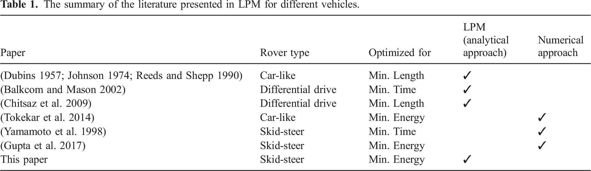
The summary of the literature presented in LPM for different vehicles.
1.2.2. Hybrid approach
Hybrid algorithms can be used to take advantage of both sample-based (for global planning methods) and analytical approaches (for local planning methods). For example, Chaudhari et al. (2014) use analytically obtained Dubins path (Dubins 1957) to have differential drive rovers traverse between the waypoints of the global path, while avoiding obstacles, obtained by A*. Although Dubins paths are the shortest path (as a LPM) for car-like rovers, using these paths obtains smoother energy-efficient paths compared to paths obtained by A* alone or even smoothed A*-paths. This raises the question of what would happen if their utilized LPM was specifically designed for energy-efficiency of differential drive rovers? In this paper, the research is not on differential drive rovers. However, to deal with similar situations for skid-steer rovers, we develop an energy-optimal LPM and thus provide the opportunity for more investigations on other related energy-optimal global planning methods.
1.3. Energy and time optimization equivalency
Solving the energy-optimal path planning problem by using its equivalent time-optimal problem is one of the main contributions of this paper. Therefore, related literature on energy-time equivalency is identified and contrasted to our approach. Possible equivalencies between time optimization and energy optimization problems have been given preliminary consideration before. Ioslovich et al. (2015, 2017) and Gutman et al. (2015) state that by selection of special constraints for a rigid body with the dynamic equations of motion (Ioslovich et al. 2017), the minimum time problem and minimum energy problem are equivalent which means that they result in the same trajectory. In their approach the final time for the energy-efficient problem is fixed as the optimal time taken from the solution of the minimum time problem. In other words, they are searching for the most energy-efficient path from among already time-optimal paths. In the case of a unique time-optimal path (not unusual in practice), this reduces to a search within a set of cardinality 1. Such a restrictive search can miss lower energy solutions that take some extra time. In this work, we do not restrict the search space (for the minimum energy problem) by taking a fixed time based on the minimum time problem.
There are also some papers that have worked on time-energy minimization in terms of a trade-off between optimal time and optimal energy (Shiller 1996; Verscheure et al. 2008; Ji et al. 2019; Zhang and Cassandras 2019; Nshama and Uchiyama 2018; Lyu et al. 2017; Faraj and Basir 2016). However, none of them work on equivalency between time and energy in their research.
1.4. Contributions
As summarized above,
The contributions of this work include the following: • The • This work finds and describes energy-optimal local paths (29 trajectory structures) for skid-steer rovers under the practical assumptions elaborated in the next section. • Another contribution is further exploration of the
2. Problem statement
Firstly, the energy-optimal path planning problem is defined. The solution to this problem is sought for any and all proper velocity constraints (as will be defined later in Definition 3, and will be shown to not limit the solution search space in any way). Then, it is proved that there exist optimal trajectories for the optimal path planning problem. Afterwards, a well-known existing power model for skid-steer rovers is introduced and analyzed. This power model is utilized for all the analysis in this paper.
2.1. Problem
The problem is to find an The general arc-based path (non-predefined class of paths) with the specified start and end pose.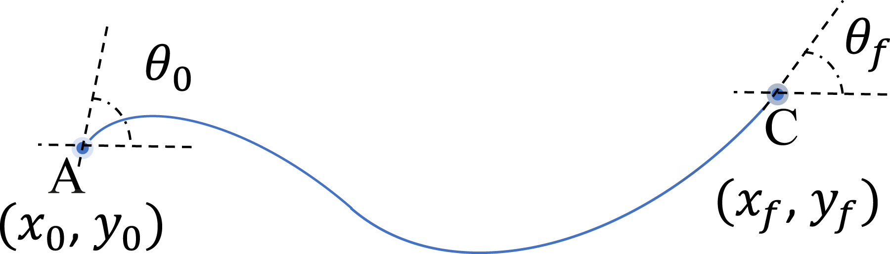
The optimization problem is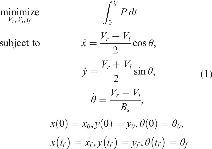
Assumptions: • The rover is skid-steer • The rover can do point turns or go forward or backward with any turning radius • The rover moves on hard flat ground • There are no obstacles • The rover center of mass is located at its centroid • The trajectory is piecewise continuous • Recall that no specific velocity constraints are required. Practical constraints to consider include motor saturation (|V
r
| < vmax, |V
l
| < vmax), constant vc (see Figure 4), and velocities that maintain constant power.
2.2. Existence theorem
The existence of optimal trajectories was originally stated by Soueres and Boissonnat (1998) (Theorem 2 on page 99) and used by Furtuna (2011) (subsection 3.4 on page 16). The theorem is slightly restated to make notation consistent with this paper:
There exists an optimal trajectory for the control set of U from 1. There exists a function g( 2. g( 3. The control set U is a compact convex subset of 4. There exists an admissible trajectory from 5. There exists a corresponding trajectory
In the following, it is easily proved that the skid-steer rover verifies the conditions: 1. As it is indicated in (Equation (1)), for a skid-steer rover 2. sin θ and cos θ are Lipschitz continuous.
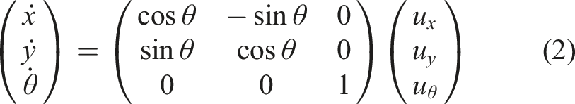
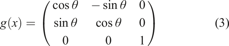
Therefore, g(x) is locally Lipschitz continuous. 3. For the problem mentioned in (Equation (1)), the considered U is a closed convex control space. 4. A skid-steer rover can travel from any starting pose to any end pose by doing a Point turn - Line - Point turn (PLP) maneuver. Therefore, there always exists an admissible trajectory. 5. From equation (2) it is known that
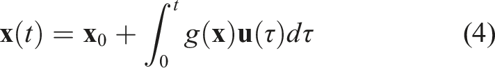
The integral in equation (4) always exists because
2.3. Power modeling
The kinematics for skid-steer rovers are presented and then incorporated into a popular existing power model.
2.3.1. Skid-steer rovers kinematics
Rover kinematics can be defined based on the concept of Instantaneous Centers of Rotation (ICR) (Mandow et al. 2007). The parameters (x
ICRv
, y
ICRv
), (x
ICRr
, y
ICRr
), and (x
ICRl
, y
ICRl
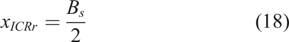
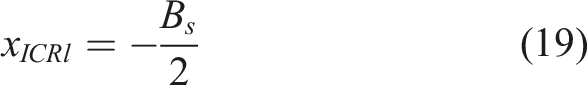
) are the vehicle, right hand-side, and left hand-side ICR positions, respectively. These parameters are shown in Figure 2 and are as follows: A schematic figure of a skid-steer rover and its associated instantaneous centers of rotation (ICRs).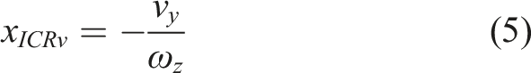
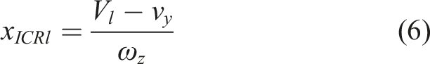
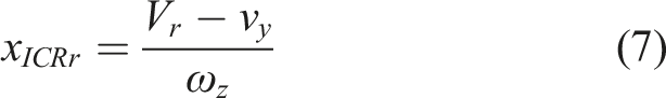
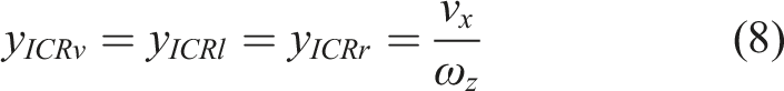
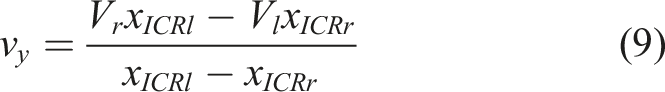
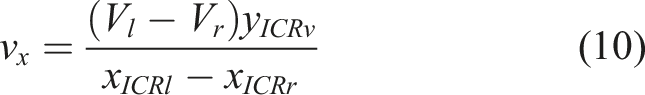
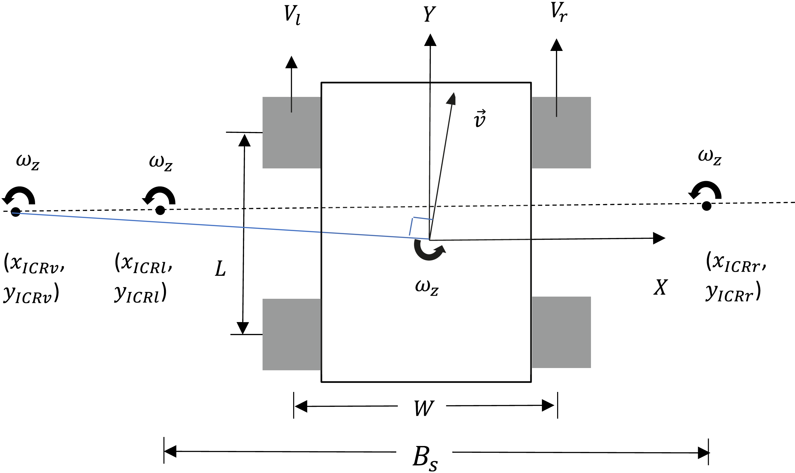
where vx, vy, and ωz are the velocity in X, velocity in Y, and angular velocity around the Z axis of the rover’s body frame, respectively. Recall that Vr and Vl are the right and left wheel velocities (i.e., wheel angular velocities multiplied by wheel radius), respectively, and are control inputs. Martínez et al. (2005) show that the positions of ICRs can be assumed to be approximately constant for a particular terrain type; although these are in fact dynamics-dependent in general, they show them to be bounded for skid-steer rovers on hard flat ground traveling at “moderate speeds,” 1 which is an operating principle to keep in mind when weighing the validity of this kinematic approach for particular applications. ICRs can be estimated by taking experimental measurements or via dynamics simulations, for a particular soil type and narrow range of speeds.
W and L are the distance between the center of left and right wheels in the X direction and the distance between the center of front and rear wheels in the Y direction, respectively. Also, the slip track (B
s
) is defined as follows:
Based on the assumptions listed in the problem statement, the rover center of mass is located at its centroid. Accordingly, the following equations are derived:

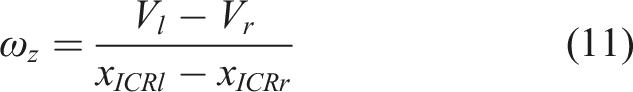
From equation (9) through equation (14) we conclude that
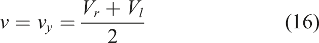
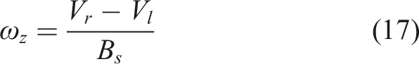
From the fact that |v| = R|ω
z
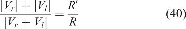
| as well as equations (16) and (17), the turning radius can be expressed as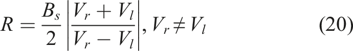
R = R′ is the boundary between the separate cases where V
r
and V
l
are either of equal or opposite sign.
R′ is the turning radius at which a skid-steer rover’s inner wheels are not commanded to turn. Without loss of generality consider the right wheel as the inner wheel. Therefore, at R′ the right velocity is zero (V
r
= 0).
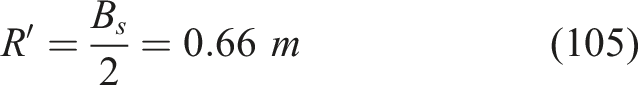
By using equation (20) the following relation for R′ is obtained: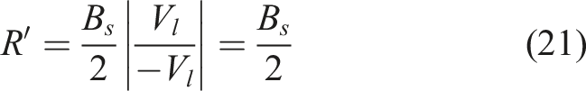
■
R′ is half of the slip track
Note: Based on Martínez et al. (2005), the positions of left and right ICRs are bounded and may be assumed constant for a specific terrain. Therefore, B s (Equation (12)) and R′ are constant.
2.3.2. Power model
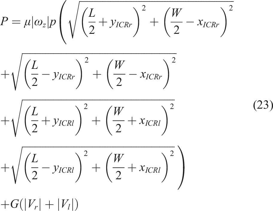
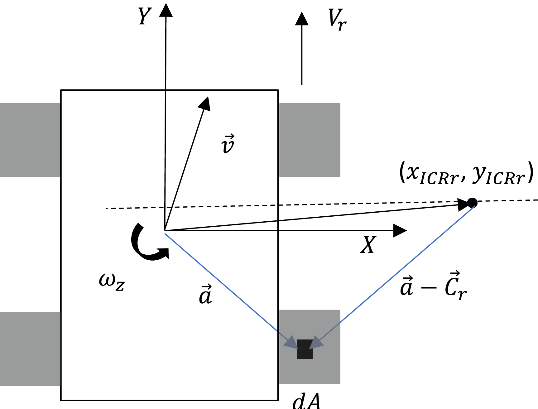
A popular power model, based on a frictional wheel-terrain contact assumption, developed by Morales et al. (2010, 2009) and used by Pentzer et al. (2016, 2014), is adapted here for usage according to the problem definition and assumptions given in the previous section. The power model is as follows: Distance of a wheel from ICR for a skid-steer rover. To calculate 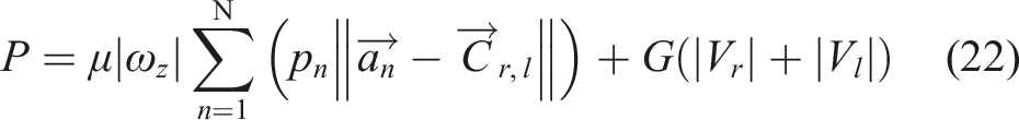


3. Equivalency theorem
The Equivalency theorem (Theorem 1) shows that all minimum-energy trajectories follow the same path irrespective of control constraints on the skid-steer rover, as long as these constraints do not prevent the rover from driving forward and backward along straight lines or with any turning radius (including a turning radius of 0, or point turn). This non-intuitive result stems from the fact that for the defined power model, the total energy is fully parameterized by the geometry of the path alone, as will be shown in Lemma 2. In this paper, the theorem is utilized to obtain an equivalent time-optimal problem. The equivalent problem will be solved to obtain the optimal path, which is the general answer to the energy-optimal path planning problem as well.
A general path is a sequential set of connected point turns, straight lines, and/or curves parameterized by R(s).
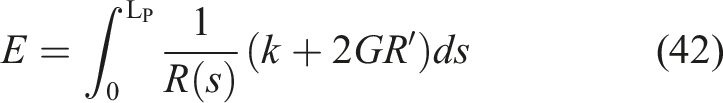
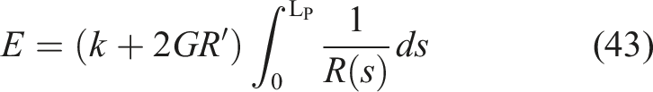
Energy (E) can be obtained by the following equation.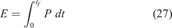
These relations are now used to show that the energy for a skid-steer rover following a general path can be written as a function of geometric path parameters of Δθ, Δs, and R(s).
The energy for the skid-steer rover when following a general path (Figure 1) while using the power model of Equation (25) is equal to: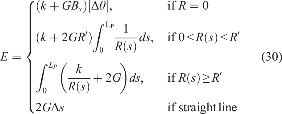
The energy for each interval of R is proved separately.
(I) R = 0:
Starting with the power model, equation (25), and the general equations (27) and (28), gives: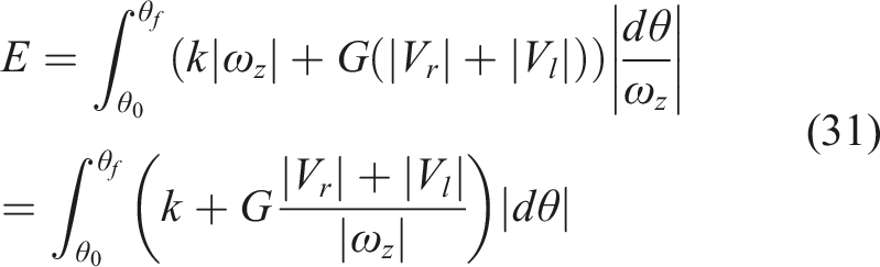
Using (17), this becomes: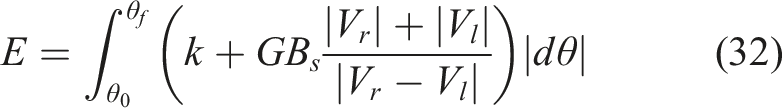
The definition of R′ ensures that for R = 0, V
r
and V
l
are of opposite sign. Therefore, the following relation can be verified:
Hence, the energy is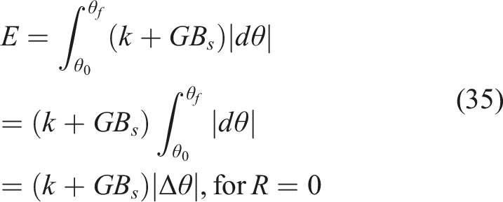
Therefore the energy for any turn with R = 0 is a constant times |Δθ|.
(II) 0 < R(s) < R′: Starting with the power model, (25), and the general equations (27) and (29), gives: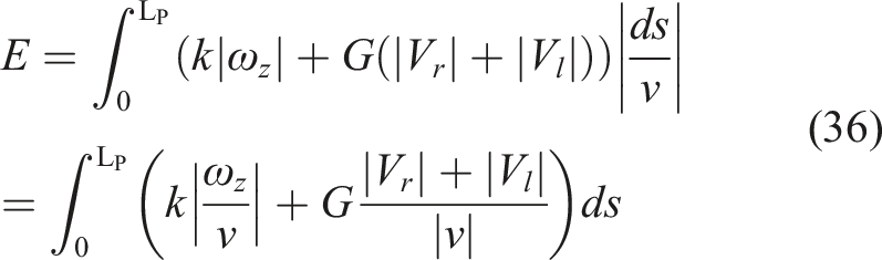
Using equation (16), this becomes: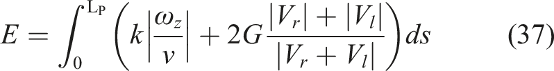
Since V
r
and V
l
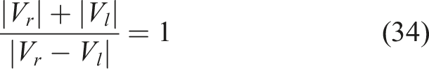
have the opposite sign in 0 < R(s) < R′, the following relation can again be verified:
Therefore, using equation (20), the following relations are obtained: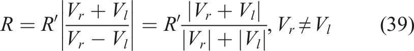
Also, |v| = R|ω
z
|. Therefore,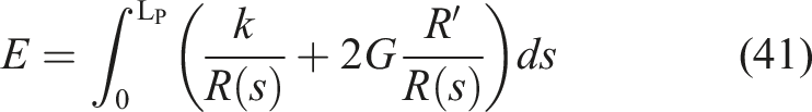
(III) R(s) ≥ R′:
Since V
r
and V
l
have the same sign, the following relation can be easily verified:
So, the following relation is true:
Also, |v| = R|ω
z
|. Therefore, using equation (37):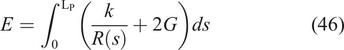
(IV) Straight line:
In the specific case of a straight line V
r
= V
l
, ω
z
= 0 and thus
A key aspect of the power model that is fundamental to the above lemma is that power is proportional to speed (as represented by |ω z | and (|V r | + |V l |) in equation (25)). In such a case, doubling speed, for example, halves the operation time but doubles the instantaneous power consumption, leaving the energy integral unchanged along any given path. Another key consideration is the assumption of co-location of centroid with center of mass; without this, equations (20) and (37) do not simplify cleanly, and the analyses in (II) and (III) above would become progressively less valid the larger the deviation from this assumption.
The lemma will be used to prove the equivalency theorem (see Theorem 1).
A • Constant vc (|V
l
| + |V
r
| = 2vc, where vc is constant) • |V
i
| < |vmax|, i = {r, l} and vmax is constant • Any arbitrary but finite velocities • Constant power velocity constraint (see Figure 5)
These velocity constraints are kinematic by definition. They do not consider the possibility of motor torques saturating due to loading conditions, which could impose additional limitations for some rovers. However, given that skid-steer rovers tend to be designed with substantial maneuverability capabilities such a case would not be expected to be encountered during nominal (e.g., payload within rated limits) operations on hard flat ground.
Optimal controls are a solution
An optimal path is the general path produced by applying optimal controls
As can be seen in Lemma 2, the energy consumption along a general path while using the power model of equation (25) can be fully parameterized by geometric path parameters (Δθ, Δs, R(s)) and is not directly dependent on V
r
, V
l
. This is the crucial aspect of the structure of the power model that enables the Equivalency Theorem. In the case of considering any alternative power model, the Equivalency theorem would also hold if the model shares this feature of geometrically parameterized energy consumption (likely for models where power is proportional to speed).
Also, any general path can be achieved by a skid-steer rover with a proper velocity constraint. This follows directly from the definitions of a general path and a proper velocity constraint, respectively.
There are no general paths that can result in lower energy consumption than an optimal path. Furthermore, a proper velocity constraint ensures that controls generating any such hypothetically lower-energy general path would have been included in the search space.
An energy-optimal path is thus energy-optimal regardless of velocity constraints, as long as the velocity constraints are proper. Only the particular optimal controls used to follow such an optimal path vary between problems with different proper velocity constraints.■
In the following, more explanations are provided to clarify Theorem 1. Based on equation (20) the turning radius is a function of the control inputs. Therefore,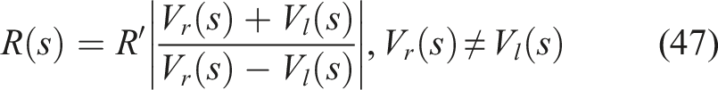
Also, from the equation for R(s), in the case of any arbitrary but finite velocities there are infinite {V l (s); V r (s)} that can produce a R(s), that is all the {aV l (s); aV r (s)} for the real number a ≠ 0 produce the same R(s).
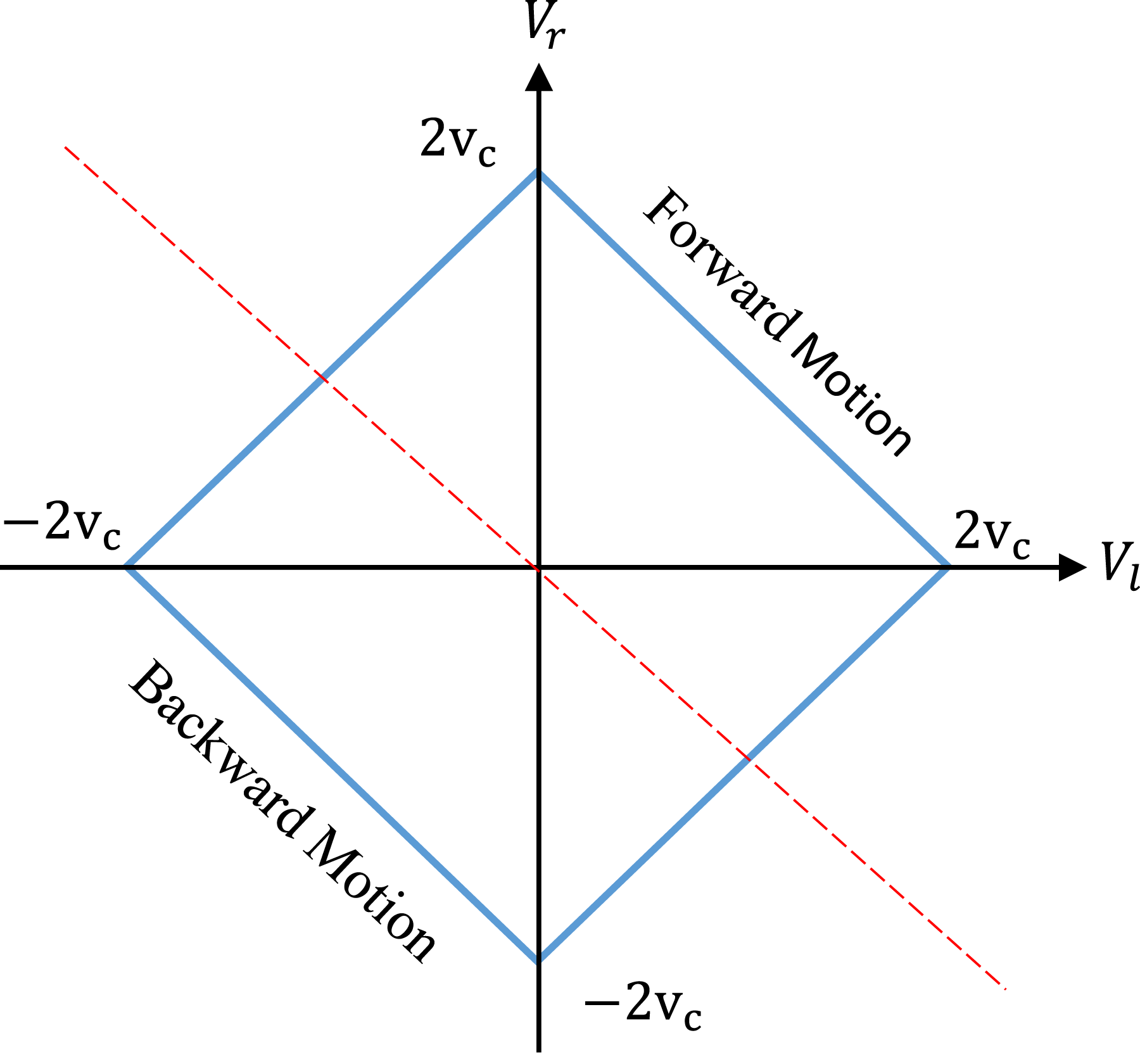
The next step is showing that the velocity constraints do not limit the R(s) values and are thus proper. Each example constraint considered is evaluated separately in the following: 1. Constant vc: Using the related figure (see Figure 4) and the equation for the turning radius (equation (20)) it is evident that for (V
l
, V
r
) ∈ {(−vc, vc), (vc, − vc)}, the turning radius is zero (R(s) = 0). In addition, when (V
l
, V
r
) is infinitesimally close to the middle of line segments in the first or third quadrant of the figure (i.e., (V
l
, V
r
) ≊ (vc, vc) or (−vc, − vc)), the turning radius approaches to infinity (R(s) → ∞) and is a straight line at the exact equality. For other values of V
l
and V
r
, the range of (0, + ∞) will be obtained for R(s). 2. |V
i
| < |vmax|, i = r, l: Using equation (20), when V
l
= −V
r
, the turning radius is zero (R(s) = 0). Also, when V
r
and V
l
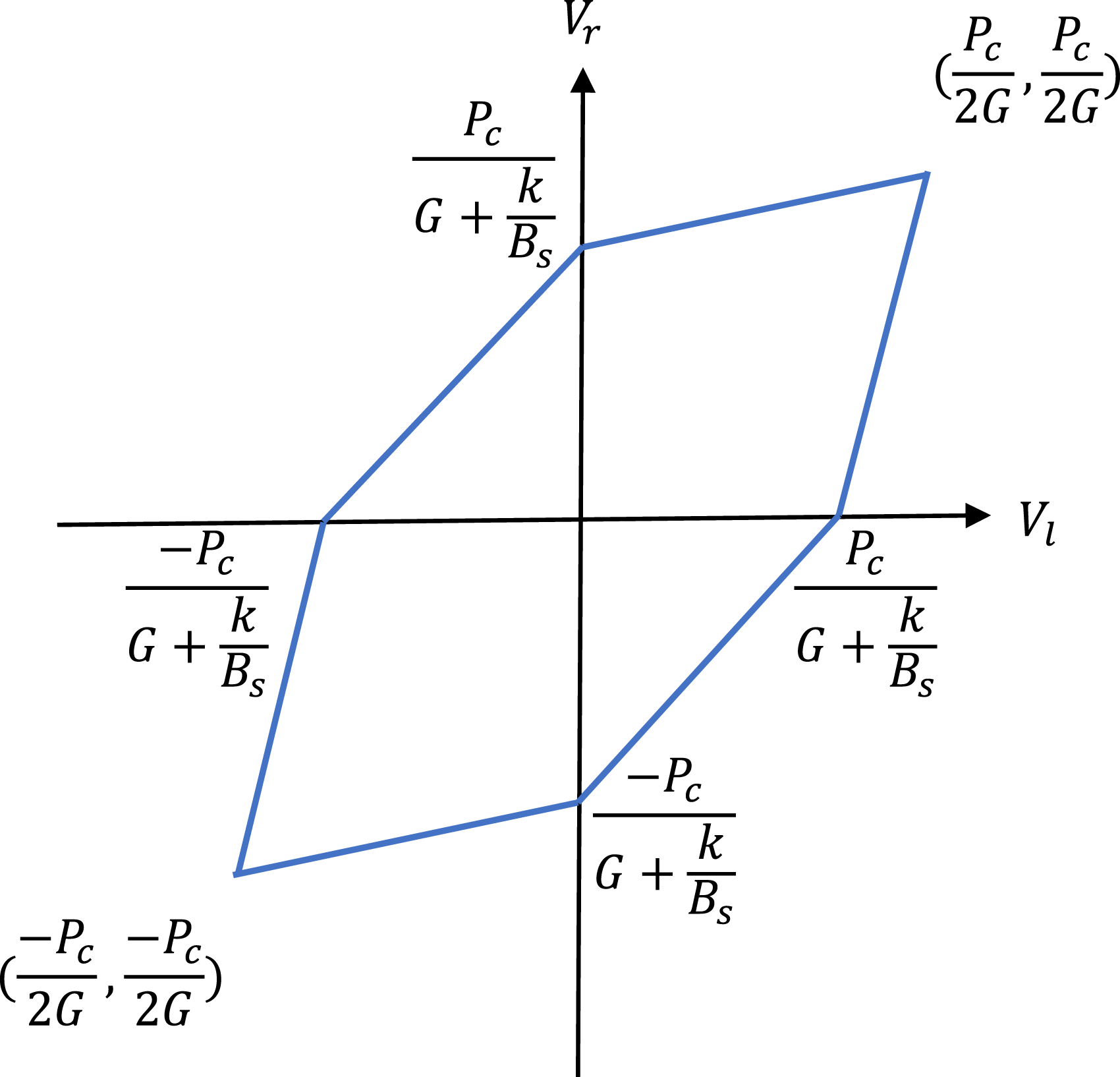
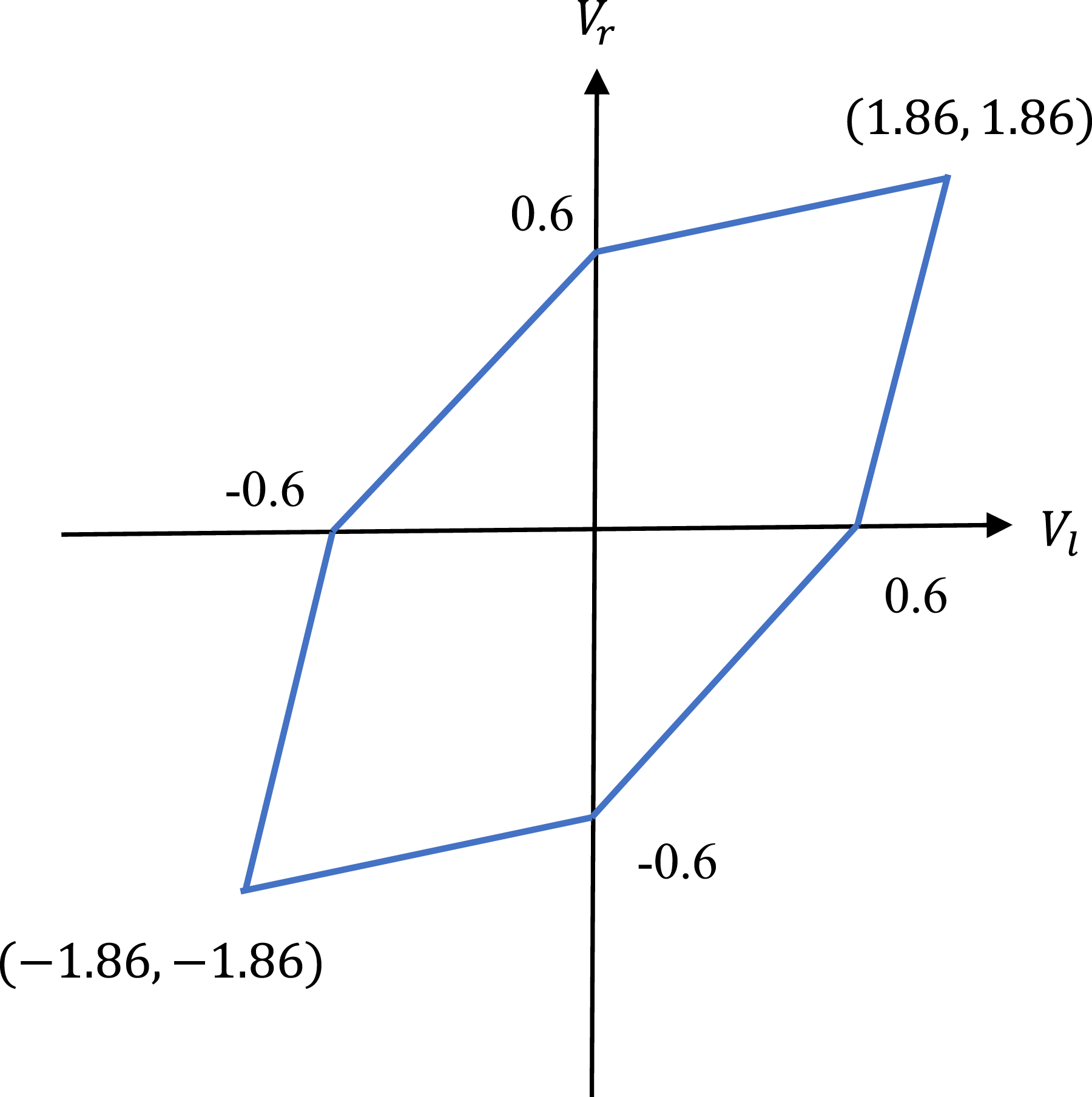
are almost equal, the turning radius approaches infinity (R(s) → ∞) and when they are exactly equal the rover follows a straight line. 3. Any arbitrary but finite velocities: The similar explanation in Part 2 is applicable for arbitrary but finite velocities. 4. Constant power: It is proven in the Appendix that to have constant power (P = Pc where Pc is a constant), V
r
and V
l
have the symmetric control space shown in Figure 5. By considering Figure 5 and equation (20), when (V
l
, V
r
) is the middle point of line segments in second or fourth quadrant of the figure
2
, the turning radius becomes zero (R(s) = 0). In addition, when (V
l
, V
r
) is infinitesimally close to the middle of line segments in the first or third quadrant of the figure (i.e., The control space obtained from Control space for the constant power of
This means the same path that is optimal for constant vc, is optimal for |V i | < |vmax| (i = r, l), is optimal for any arbitrary but finite velocities and is optimal for constant power velocity constraints.
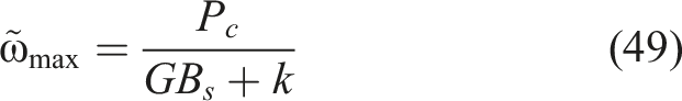
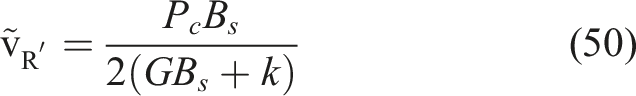
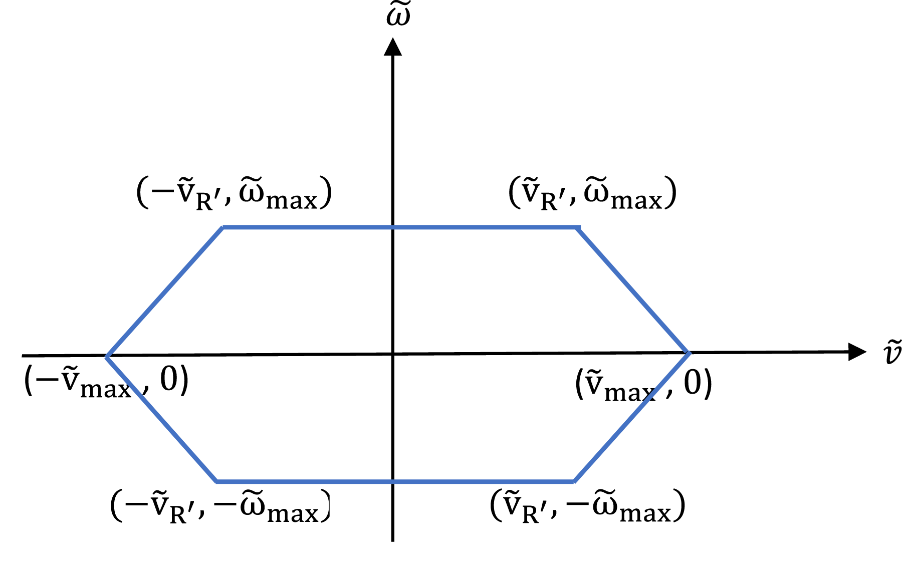
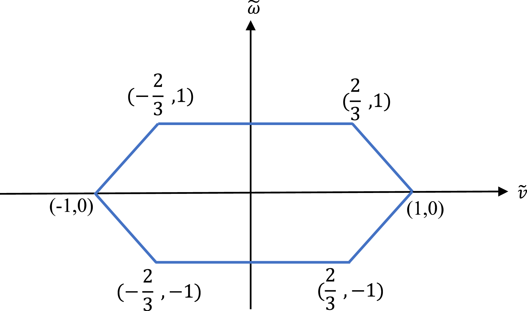
By using equation (16) and equation (17), Figure 6 is obtained from a re-parameterization of Figure 5. The parameters in Figure 6 are as follows: Control space of a (constant power) skid-steer rover for the equivalent time-optimal problem.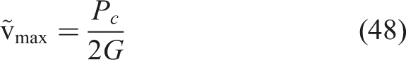
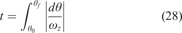
Accordingly, to solve the energy-optimal path planning problem (see equation (1)) there are two approaches: 1. To directly apply Pontryagin’s Minimum Principle and then prove several theorems specified for skid-steer rovers to obtain all the extremal paths for the energy-optimal path planning problem: In this approach theorems and processes analogous to those performed by Furtuna (2011) should be regenerated and then be revised/adjusted for our problem (equation (1)). Furtuna (2011) proves several theorems for time-optimal path planning of a rigid body. These theorems are for obtaining the extremal control inputs, categorizing different type of paths, limiting the number of extremals, determining the switch points of the extremals, and defining length/periodicity of the correspondent extremal paths. 2. To use the “constant power” constraint and find an equivalent time-optimal problem for the energy-optimal problem (equation (1)): Based on the equivalency theorem, “constant power” is one of the several proper constraints that may be considered to obtain the optimal path for the energy-optimal path planning problem. Accordingly, the constraint can be used to convert the energy-efficiency to an equivalent time-efficiency problem. From equation (27) it is known that
In this paper, the second approach, which is considering “constant power” and its related velocity constraints, is utilized to solve the energy-optimal path planning problem (see equation (1)). This is not the same as simply solving the time-optimal problem for skid-steer rovers in general. The energy-optimal solution is only found if the particular “constant power” velocity constraints (Figures 5 and 6), derived here, are considered; these constraints would not reasonably be applied if one were interested in finding the actual time-optimal paths.
Accordingly the following equivalent time-optimal problem is defined:
Equivalent time-optimal problem: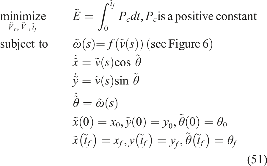
3. Extremal trajectories for the equivalent time-optimal problem
Firstly, Pontryagin’s Minimum Principle for time-optimal problems is presented. This theorem is required to obtain Hamiltonian level sets. Then, the optimal control inputs are calculated by the use of a theorem presented by Furtuna (2011). Hence, the Hamiltonian level sets are used to graphically analyze and categorize the extremal paths. Finally, explanations are given to restrict the number of periods and thus give the complete table of the extremal path structures. These finite number of extremal path structures will be enumerated and compared to find the optimal solution.
3.1. Pontryagin’s minimum principle for time-optimal problems
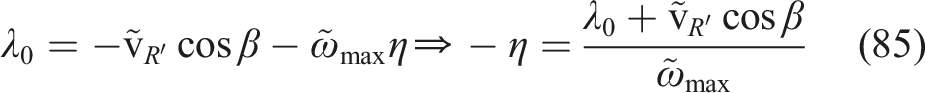
Pontryagin’s Minimum Principle for time-optimal problems (Theorem 2) is presented by Pontryagin et al. (1962). This theorem is required for this research to • define the Hamiltonian • use the concept of constant maximum of negative Hamiltonian (minimum of Hamiltonian), λ0 in equation (76), to obtain the Hamiltonian level sets.
Let

A nontrivial continuous adjoint function of 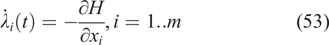

Conditions for optimality:
(I) For all t, t0 ≤ t ≤ t1, the maximum of −H(
(II) M(
The proof of the theorem is presented by Pontryagin et al. (1962).■
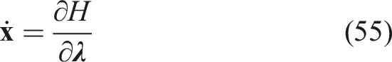
The following relations for the first derivatives of the states are known:


Note: For notational simplicity, the time variable is omitted in the following relations and variables.
Using Equation (54) and Equation (58) through equation (60) gives the following relation for the Hamiltonian:
Also, using equation (53) gives:
After integrating to solve for λ:

Substituting equation (63) into the Hamiltonian results in the following relation:
Pontryagin’s Minimum Principle indicates that the adjoint equation (equation (53)) cannot be identically zero. In other words, c1, c2, and c3 are not all zero. Hence, the following two cases are considered: 1. c1 = c2 = 0 2. One of c1 or c2 is not zero. For simplicity and without loss of generality it is assumed that
The paths that are obtained for the case when c1 and c2 are both zero, are called whirls by Furtuna (2011), and the rest of paths are non-whirls. Whirls for a skid-steer rover have a maximum value of angular velocity almost everywhere (|ω
z
| = 2vc/B
s
) while their speed (|v|) is in [0, vc]. This is equivalent to paths with maximum |ω
z
| when R ∈ [0, R′]. The structure of whirls consists of rolls and a catch (Furtuna 2011). The rolls are circular arcs with R = R′. The catch part is a circular arc of
In the following the second case is investigated when the following condition is held:
For a line in the plane given by the equation ax + by + c = 0, where a, b, and c are real constants with a and b not both zero, the perpendicular distance of a point (x0, y0) from the line is as follows (Spain 2007):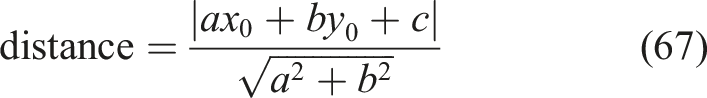
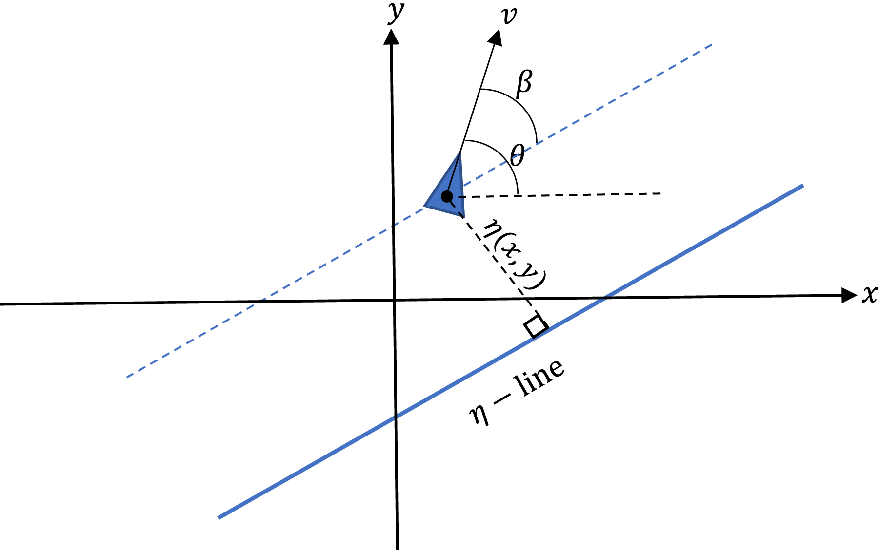
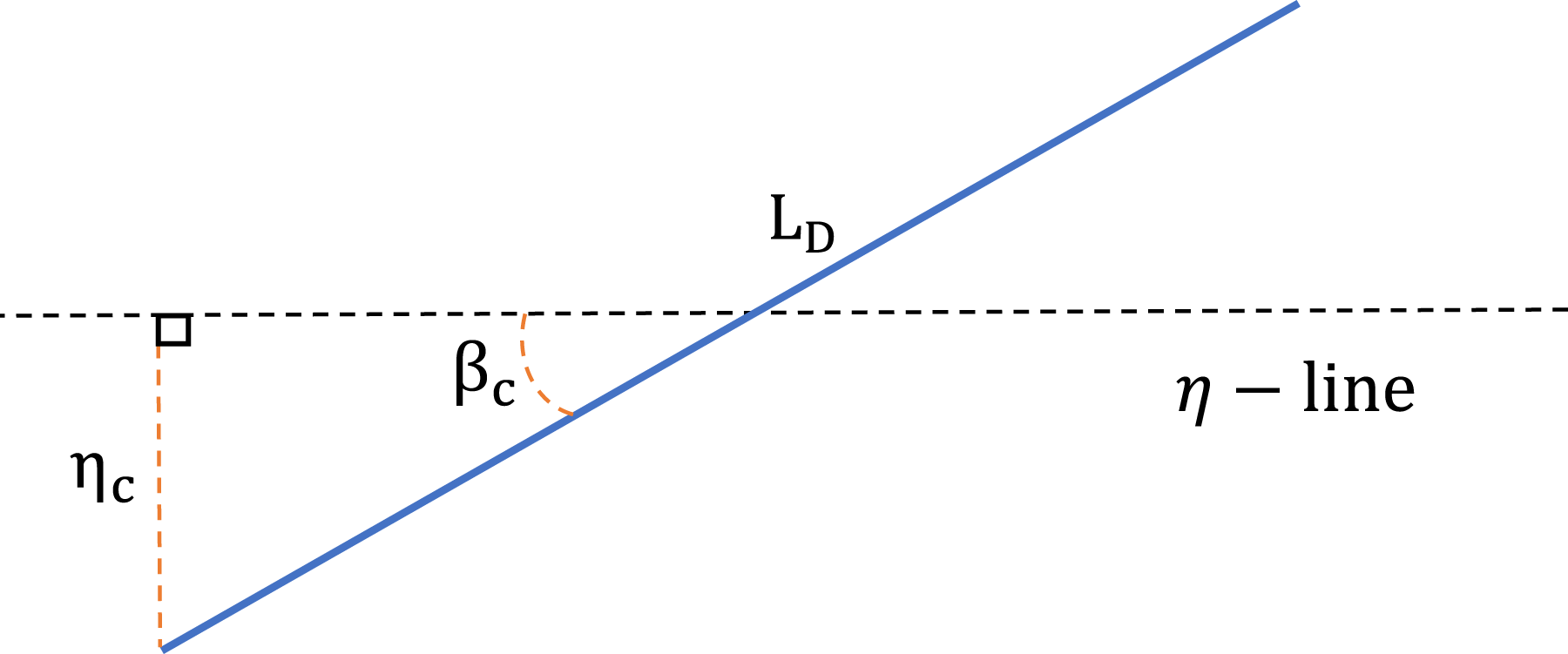
Considering equation (64) for η(x, y), assuming equation (66), and using Lemma 3, it is concluded that η(x, y) is the signed distance of the robot’s centroid from a line which is named the η-line, following a convention from Balkcom and Mason (2002). Also, the η-line is named control line by Furtuna (2011). For simplicity it is assumed that the center of mass and centroid of the robot are the same. The η-line (see Figure 7) is a hypothetical control line in 2D and distance to it determines the path type.
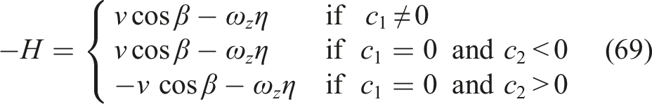
If β (see Figure 7) is defined as Equation (68), the Hamiltonian (Equation (65)) will be converted to Equation (69), while Equation (64) and Equation (66) are considered. Schematic figure to show the η-line and the related parameters. β is the orientation of rover with respect to the η-line.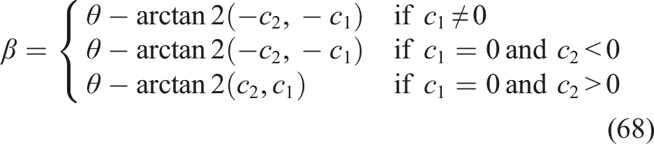
The proof for c1 ≠ 0 as well as c1 = 0 & c2 < 0 is presented by Balkcom and Mason (2002). There is a typo in equation (79) of the paper published by Balkcom and Mason (2002). It should be written in the format of β = θ − arctan2(−c2 , − c1). Then, the results presented in the paper for the mentioned conditions of c1 and c2 are valid. The only remaining part is c1 = 0 & c2 > 0 which is elaborated hereunder:
For two variables of x and y the definition of arctan2(y, x) (Betz 2015; Lenarcic et al. 2012) is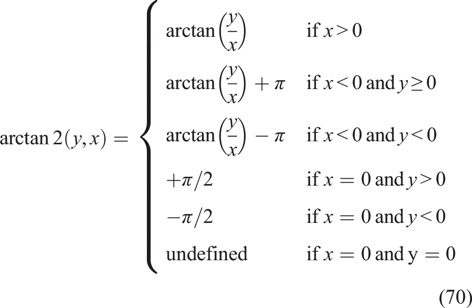
Therefore, the following relation is concluded for the condition of c1 = 0 & c2 > 0:


Also, for c1 = 0 & c2 > 0 and considering 
Equation (69) and the optimal control inputs that will be obtained in the next subsection will be used to graph the Hamiltonian level sets.
3.2. Time-optimal control inputs
The following theorem is Theorem 2 (page 29) of Andrei Furtuna’s thesis (Furtuna 2011). This theorem is utilized to obtain the optimal control inputs
The problem is time-optimal control of an autonomous rigid body and the assumptions are as follows: • moving in the Euclidean plane without obstacles; • the state vector of
• the model is fully kinematic, assuming that acceleration happens so fast that its time can be neglected. This is a common assumption for rovers of low speeds; • it is assumed that the control set U is a convex polyhedron in • U fully specifies the vehicle’s capabilities.
For the control set U, there is canonical finite subset U
c
that includes the vertices of U and at most one point on each face or edge of U that intersects the 1. is piecewise continuous 2. only takes values in U
c
The control space in Figure 6 can be convexified (converted into a convex polyhedron in 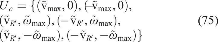
Because U
c
are all vertices of Figure 6, it is clear that convexification has not ultimately violated the original constraint. Given that Uc already includes the
3.3. Hamiltonian level sets
Firstly, the Hamiltonian level sets for the following conditions • c1 ≠ 0 • c1 = 0 & c2 < 0
are calculated. Then, the Hamiltonian level sets for c1 = 0 & c2 > 0 are explained. Hence, the Hamiltonian level sets for the equivalent time-optimal problem (equation (51) of Theorem 1) are obtained. These level sets will be used in obtaining the extremal paths.
Hamiltonian Level Sets for c1 ≠ 0 or c1 = 0 & c2 < 0: λ0 is defined as the maximum of equation (69). Therefore,

It is mentioned in Theorem 2 that λ0 is constant. Also, equation (76) is the dot product of the following vectors:

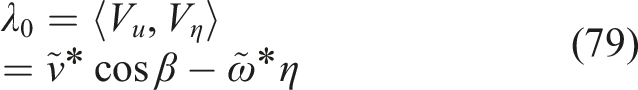
As mentioned before, λ0 is constant for the equivalent time-optimal problem. Also, 
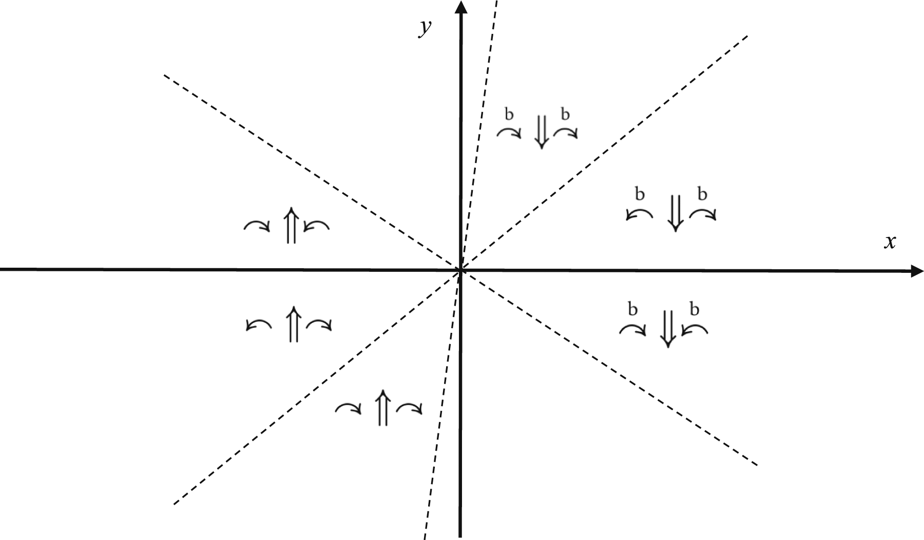
Symbols and the related maneuvers. CCW and CW stand for counter clockwise and clockwise, respectively.
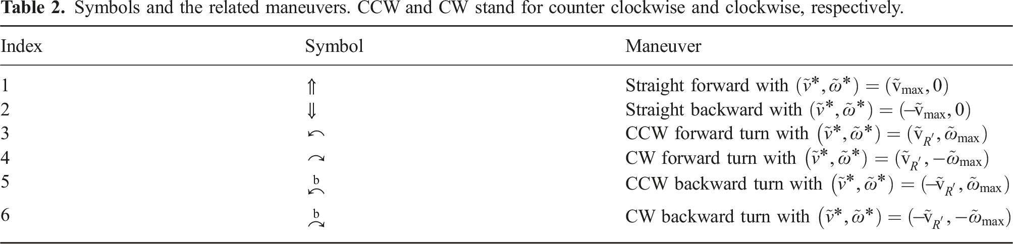
Notice that all the turns (Index three through 6) in Table 2 have the turning radius of R′ (in R′ just one of
1. 
2. 
3. 
4. 
5. 
6. 
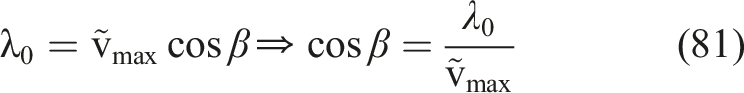
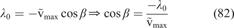
In general cos β ∈ [−1, 1]. Therefore, from equation (81) and Equation (82) it is concluded that if
(i)
Feasible Maneuvers: ↶, ↷,
(ii)
Feasible Maneuvers: ⇑, ⇓, ↶, ↷,
(iii)
Feasible Maneuvers: ⇑, ⇓, ↶, ↷,
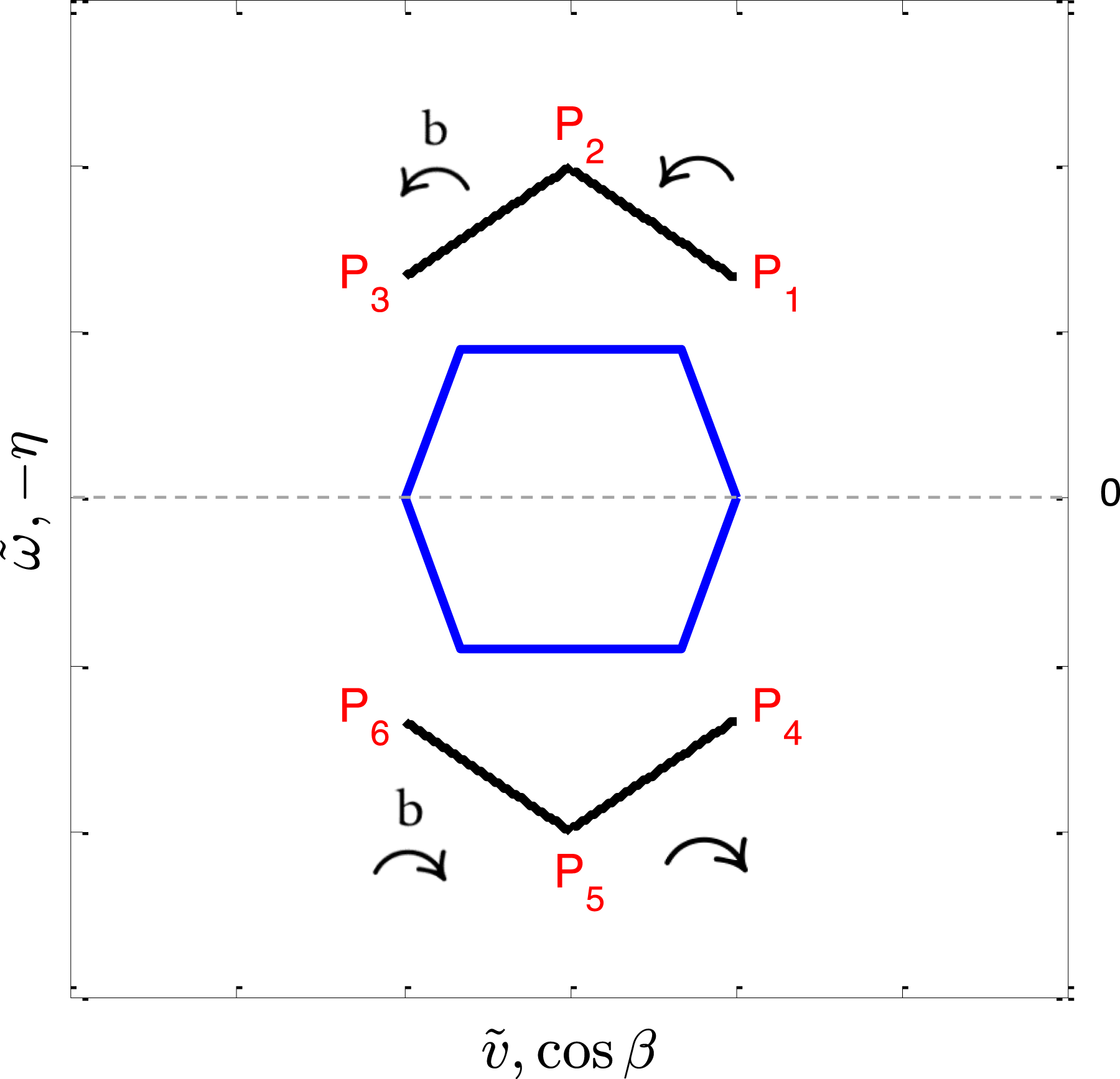
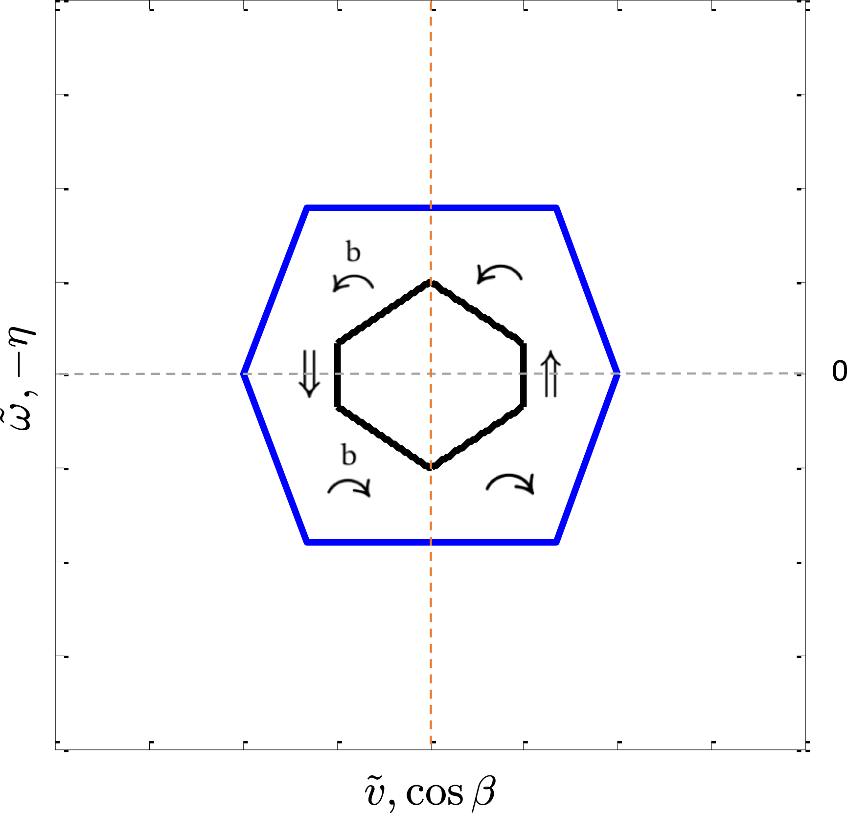
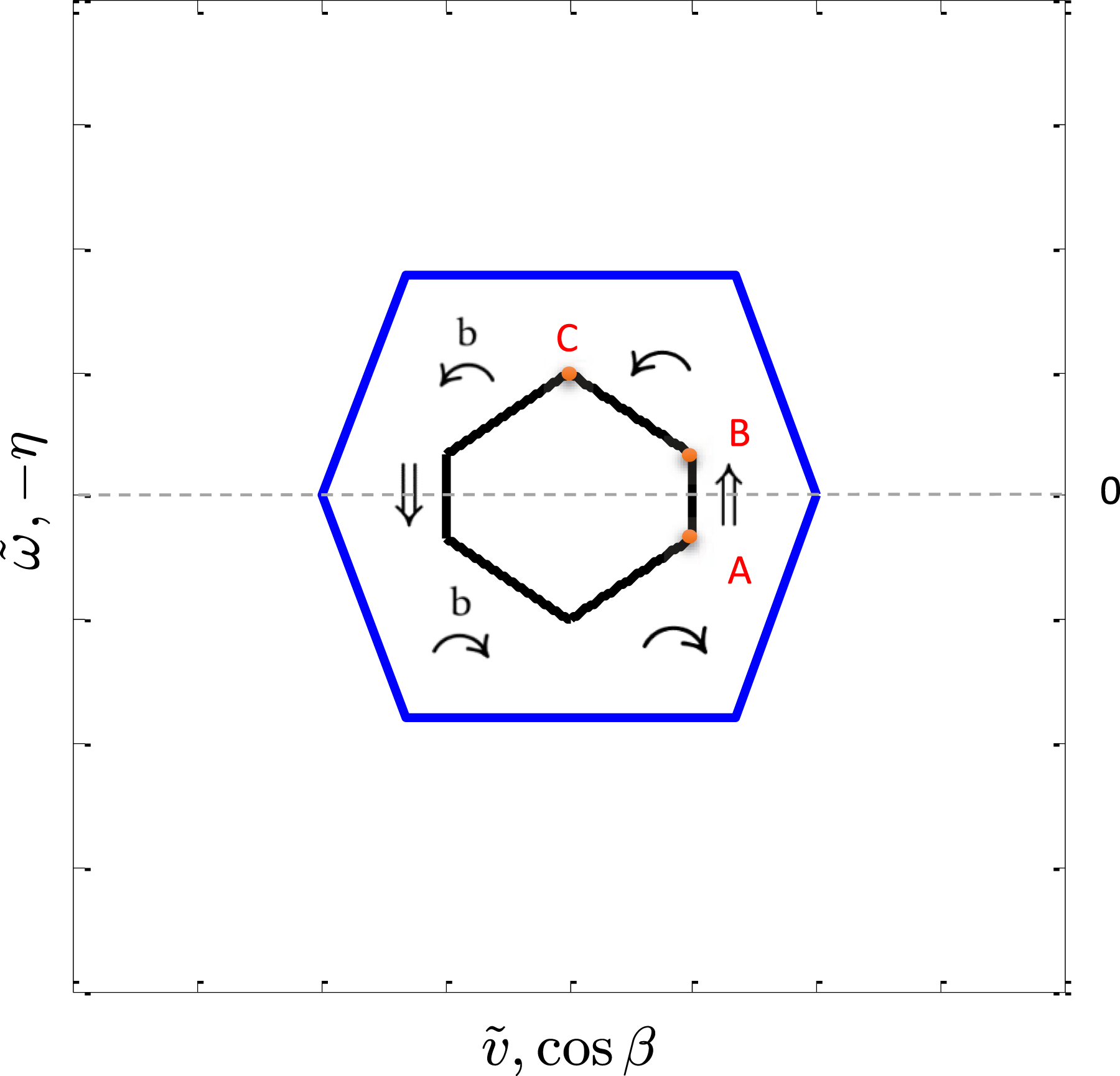
The feasible equations, considering the above categories for λ0, from amongst equation (81) through equation (86) are considered. Hence, the following conclusions are obtained for Hamiltonian level sets:
For the figures (Figure 9 through 11), the line segments of Hamiltonian level set closest to the origin are kept. Because λ0 = max(−H(t)) (see equation (76)), for the farther part of a level set’s line, there is always another line with higher λ0. For example, consider the dashed line which extends from P1P2 (level set’s line) in Figure 8. There are other level set’s lines, which are parallel to P2P3, with higher λ0, that is, the line segment that crosses the dashed line at PCross. Therefore, the dashed line segment does not satisfy Pontryagin’s Minimum Principle and should not be sketched/considered. Hence, by the similar explanation, the other line segments for the Hamiltonian level sets in Figure 9 through Figure 11 are obtained. An example to show why the level set’s lines should not be extended in Figure 9. The level set (black lines) for 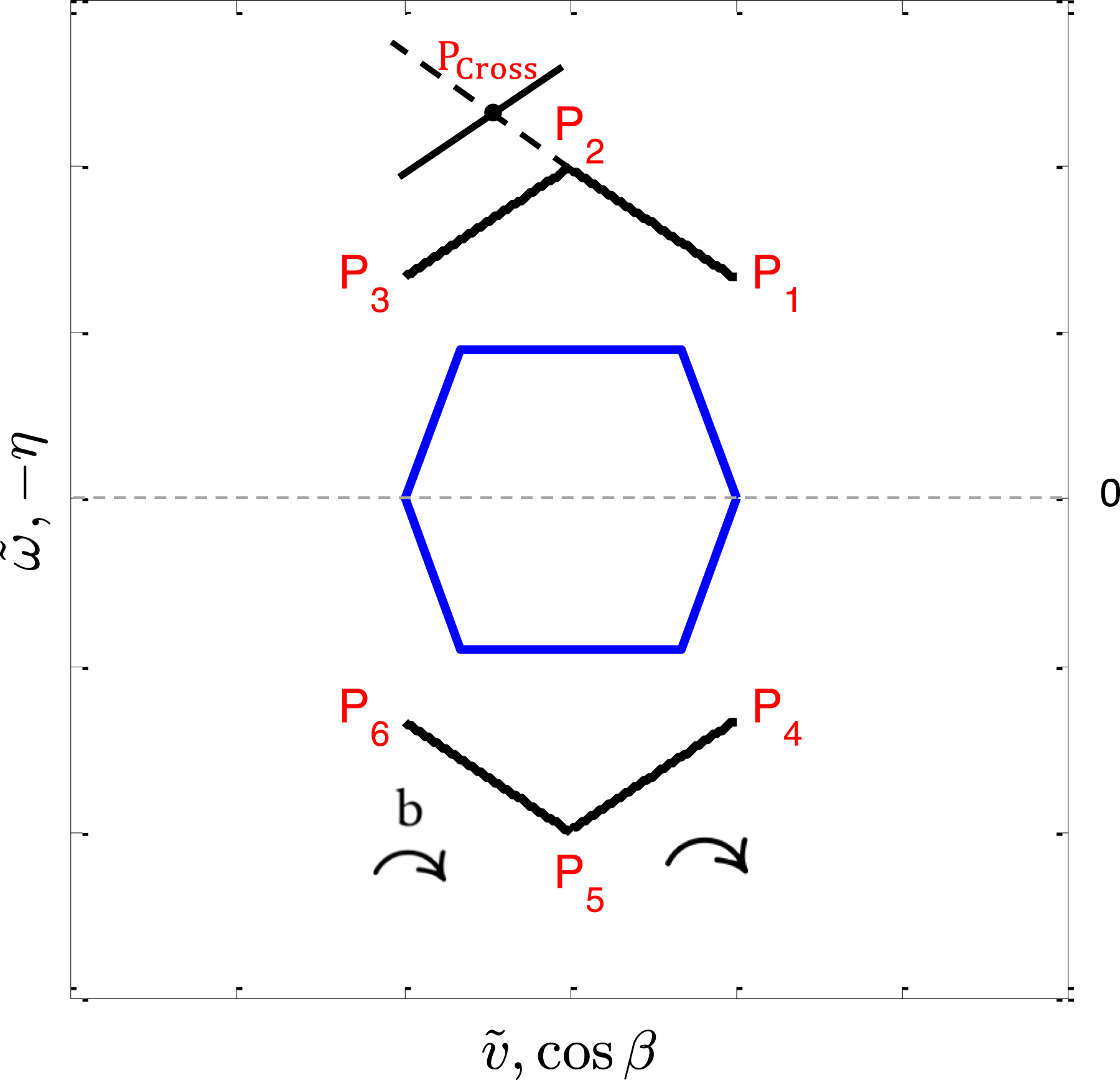
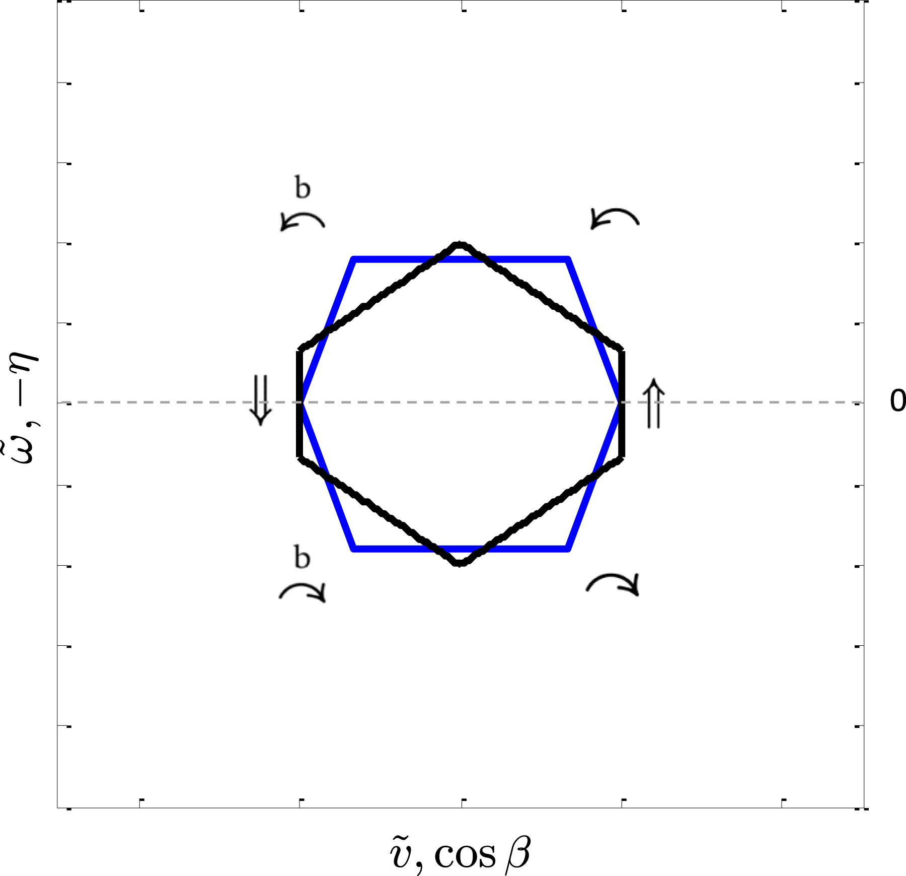
The level set (black hexagon) for
The level set (black hexagon) for
3.3.1. Hamiltonian level sets for c 1 = 0 & c 2 > 0
If the same process that was explained in the previous subsection is followed for the Hamiltonian level sets, Figure 9 to Figure 11 will be mirrored with respect to the line of cos β = 0. The reason for being mirrored is the negative sign by which cos β is multiplied (see −H equation for the condition of c1 = 0 & c2 > 0 in equation (69)). For example, in Figure 9, the hexagonal shape level set is mirrored with respect to the vertical orange line. Therefore, Figure 12 is obtained. The level set (black hexagon) for 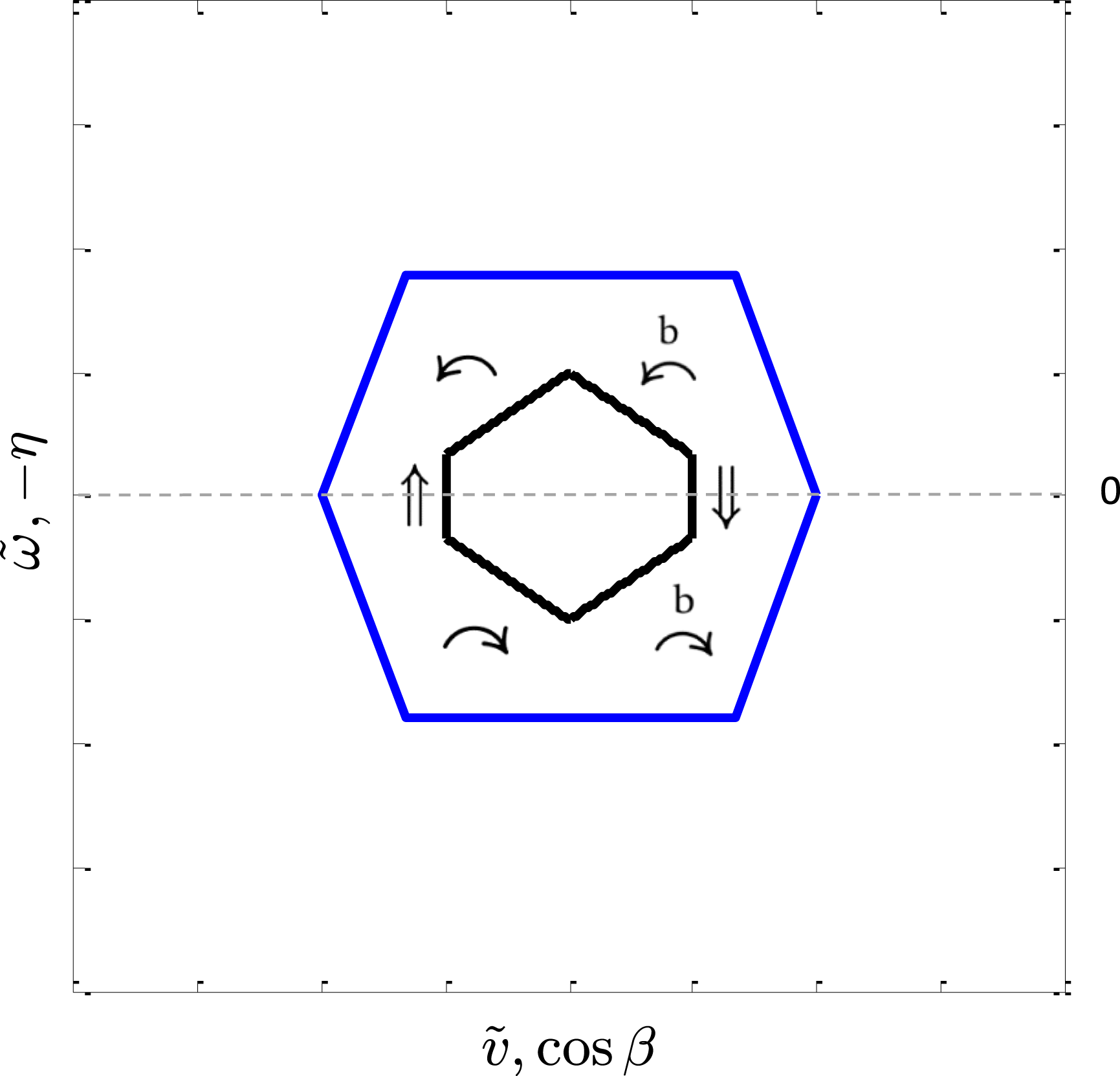
The Hamiltonian level sets will be used to obtain the shape of the extremal paths in upcoming subsections. First, some constraints on the period of the paths must be considered which are explained in the following subsection.
3.4. Restricting the number of periods for the obtained paths
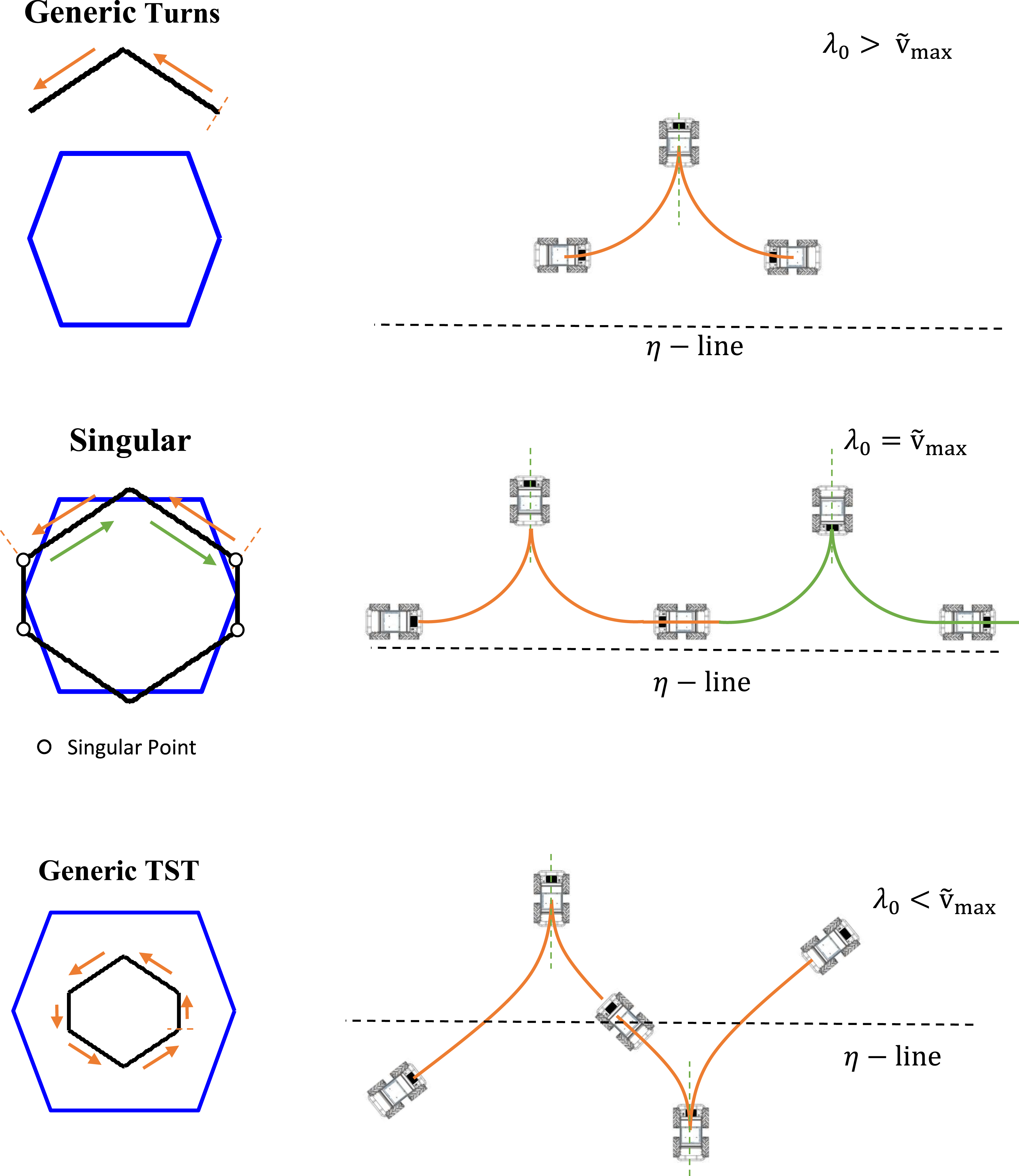
Using the obtained Hamiltonian level sets and the geometrical interpretation presented by Balkcom and Mason (2002), the extremal paths can be obtained. Actually, the distance of the rover’s centroid to the η-line determines the control policy (Balkcom and Mason 2002). Therefore, different paths that are shown in Figure 13 are obtained from the level sets that were shown in Figure 9, Figure 10, and Figure 11. As it is shown in Figure 13, there are three types of paths: • Generic Turns which consist of only turns • Singular paths • Generic TST which stands for generic paths with sequences of Turns, Straight lines, and Turns Different path types based on the λ0 categories.
The naming convention of Generic and Singular paths are adopted from the references (Balkcom and Mason 2002; Furtuna 2011).
Also, the difference between the above-mentioned paths is explained in the following:
For Generics (Generic Turns and Generic TST) the position of the η − line uniquely determines the optimal control inputs. Therefore, the paths will be unique.
However, Singulars are the paths that may include singularities. As it can be seen in Figure 13, since in the singular points the angle of the robot with respect to the η − line is 0 or 180o, the robot can maintain its straight line motions or can switch to turns at any particular point in time. Specifically, Singulars are the paths that their straight line motions (⇑, ⇓) are parallel to the η − line.
Now, by using Figure 13 all the paths will be obtained using methods analogous to those used by Furtuna et al. (2011) and Dolinskaya and Maggiar (2012). However, the period of paths can be restricted. Accordingly, the following theorems are proved/presented.
The generic (non-singular) paths contain no more than one period if the following conditions are held: 1. The image of θ(t) is not S1 2.
It is proved in page 46 (Lemma 16) of Furtuna’s thesis (Furtuna 2011).■
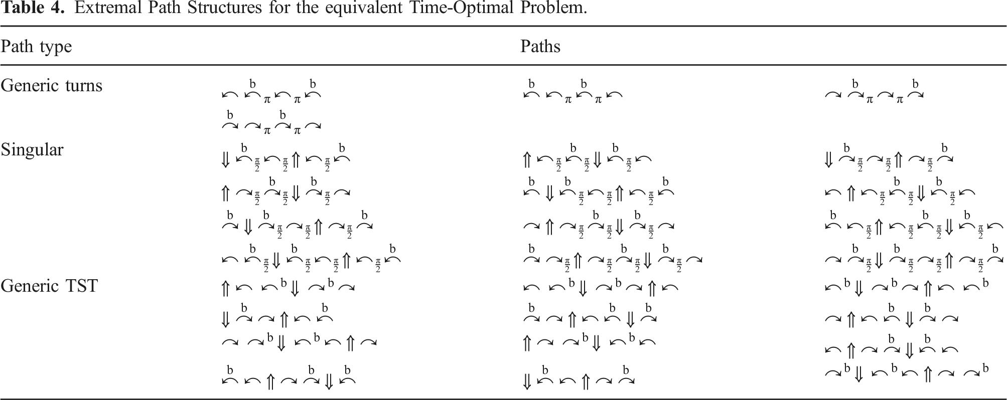
Extremal Path Structures for the equivalent Time-Optimal Problem.
the total turning angle of singular paths is less than 3π.
As it is shown in Figure 13 there are three types of singular paths, based on the starting maneuver: (I) CCLCCLCC…, that is, (II) CLCCLCCL…, that is, (III) LCCLCCLC…, that is,
where “C” stands for R′-Circular arcs and “L” stands for Lines In the following each type is elaborated separately.
(I) CCLCCLCC… • If the rotation during the initial “C” is less than • If the rotation of the initial “C” is equal to
(II) CLCCLCCL…
The maximum length optimal Type(II) path is CLCCLCC with the rotation of the final “C” less than
(III) LCCLCCLC…
The maximum length optimal Type(III) path is LCCLCC with the rotation of last “C” less than
the total turning of Generic Turns are less than 3π.
Considering Figure 13, it could be concluded that Generic Turns are analogous to Singularities but without straight line motions (⇑, ⇓). The sections that can be replaced by just straight lines always include a π/2 rotation in one direction (forward or backward) followed by a π rotation in the other direction and finally another π/2 rotation in the first direction, always in the same sense (CW or CCW), a 2π rotation in total (see Theorem 5). The maximum Generic Turn that avoids containing this particular pattern as a subset is just under 3π. Accordingly, the total turning of Generic Turns must be less than 3π. ■
3.5. Extremal path structures
From Theorem 3, the set of the optimal control inputs (Uc) is obtained. The control inputs are utilized to obtain and draw Hamiltonian level sets (Figure 9 through Figure 11). A sample for the related path to each level set is shown in Figure 13. Then, Theorem 4 through Theorem 6 are utilized to constrain the number of periods for the Generics and Singulars. Hence, Table 4 for the extremal path structures is obtained, covering all possible candidates for optimal path according to the Hamiltonian level sets. The finite number of path structures, 28, shown in Table 4 and their sub-paths are enumerated to obtain the optimal path for a given start and end pose. In the following section, a numerical scenario is solved for the above-mentioned table. In addition, some of the paths in the table are visualized.
4. Numerical scenario
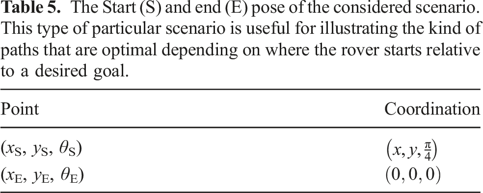
The Start (S) and end (E) pose of the considered scenario. This type of particular scenario is useful for illustrating the kind of paths that are optimal depending on where the rover starts relative to a desired goal.
4.1. Length of straight lines in generic TST paths
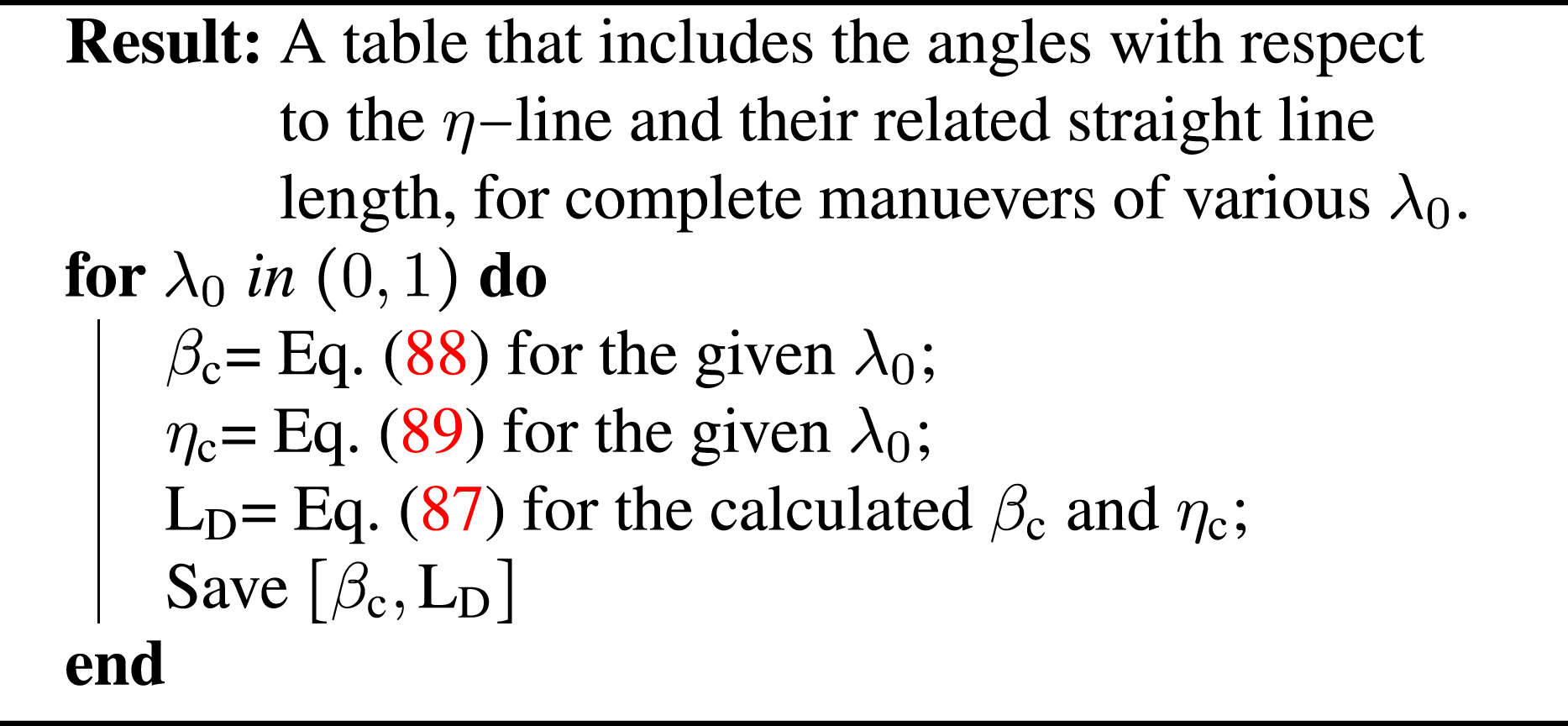
Firstly, a complete maneuver is explained in Definition 6. Then, the length of complete ⇑ or ⇓ for generic TST paths (see Figure 13) is mathematically obtained in Lemma 5.
For the maneuvers shown in Table 2, a
For example, ⇑ in Figure 14 is a complete maneuver if its related level set’s line segment includes all the points between A and B inclusive. Point A is the switching point between ↷ and ⇑. Also, B is the switching point between ⇑ and ↶.
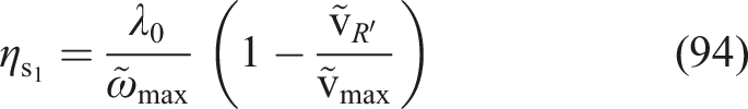
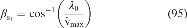
The length of a complete ⇑ or ⇓ maneuver for Generic TST paths is The level set for explaining a complete maneuver. Complete ⇑ maneuver for a generic TST path in Figure 13.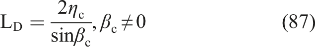
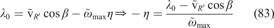
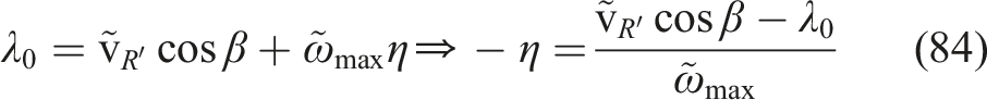
In the following, the analysis is done for complete ⇑ maneuver that the similar evaluation can be performed for complete ⇓ maneuver. From the symmetry of the level sets (Figure 13) the η − line crosses the middle of a complete ⇑. Hence, by considering Figure 14 the following relation is obtained: Therefore, Since ⇑ is a complete maneuver, ηc occurs at the switching point of ↷ ⇑ or ⇑ ↶ path. In the following each one is analyzed separately: • Switching point of ↷ ⇑ Equation (81) and equation (84) give the following relations at the switching point: • Switching point of ⇑ ↶ Equation (81) and equation (83) give the following relations at the switching point: Also, ■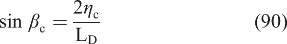
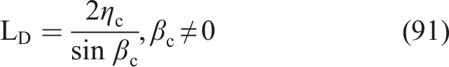


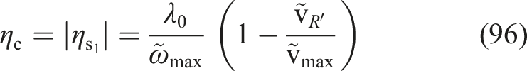


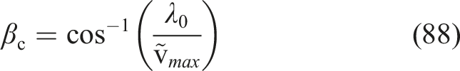
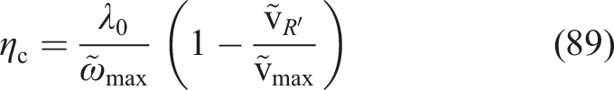
For generic TST paths:
Consider equation (87) through equation (89). If λ0 = 0, it will result in βc = The proved lemmas will be used in Algorithm 1 to create a table that includes βc and LD. Before that step, the scenario will be defined in the following subsection.
4.2. Particular scenario and steps to find the optimal paths
Inspecting Figures 6 and 16 reveals that: The example control space considered for the numerical scenario.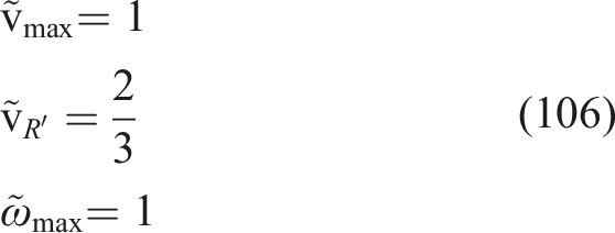
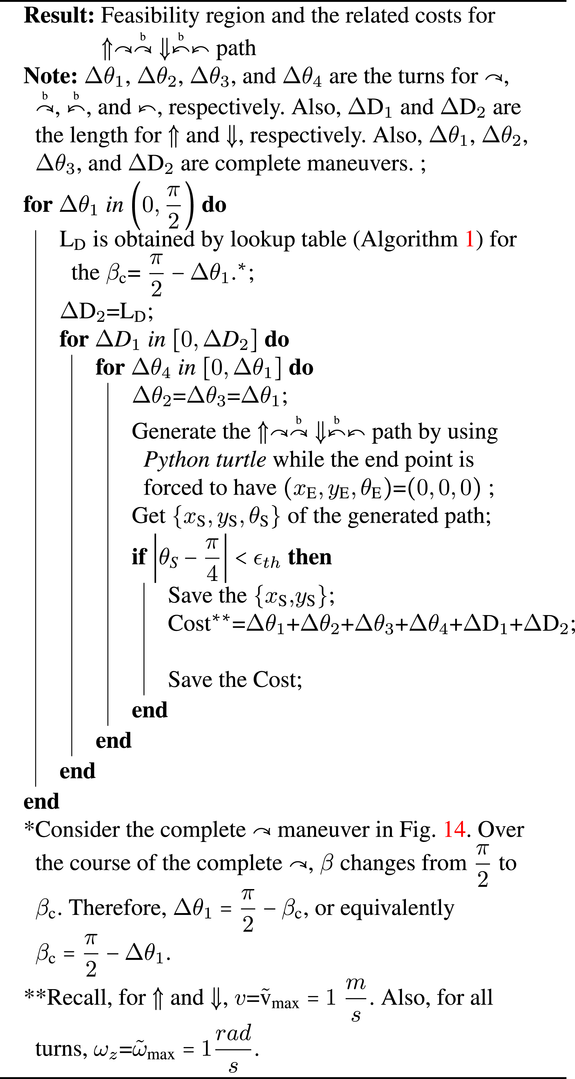
There are three main steps for producing the optimal map shown in Figure 19: I Generating all the extremal path structures reported in Table 4 and their subpaths by using turtle library in Python. II Finding the feasibility region for each of the paths for the considered scenario. Also, calculating the cost of the paths. III Comparing the cost of the paths and drawing the optimal map.
Step I and step II are explained in the following subsection. Step III is performed in subsection Map of the Optimal Paths.
4.3. Generating extremals and finding the feasibility regions
An example for a generic TST path is plotted in Figure 17. The path is generated by using turtle library in Python.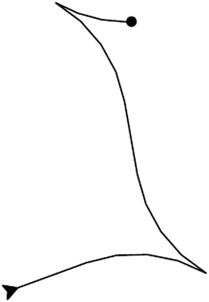
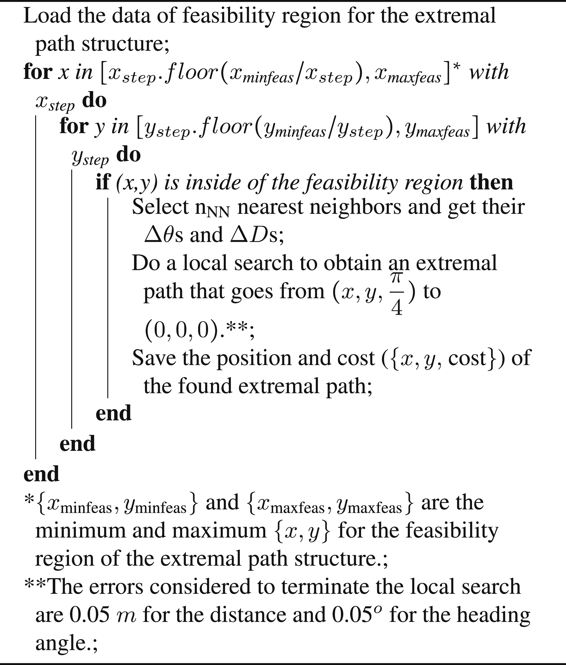
As an example the algorithm utilized to obtain the feasibility region/line for the path (and its subpaths) shown in Figure 17 is explained. The algorithms of all remaining paths and their subpaths are obtained with similar methodology.
Algorithm 1 uses Lemma 5 to generate a table including LD and the related βc. The table produced by this algorithm is used in Algorithm 2 which calculates the feasibility regions for subpaths of Figure 17 (an example of generic TST paths). In all these cases, subpaths are defined such that the first and last maneuvers need not be complete (by Definition 6).
Resulting feasibility region for all subpaths of 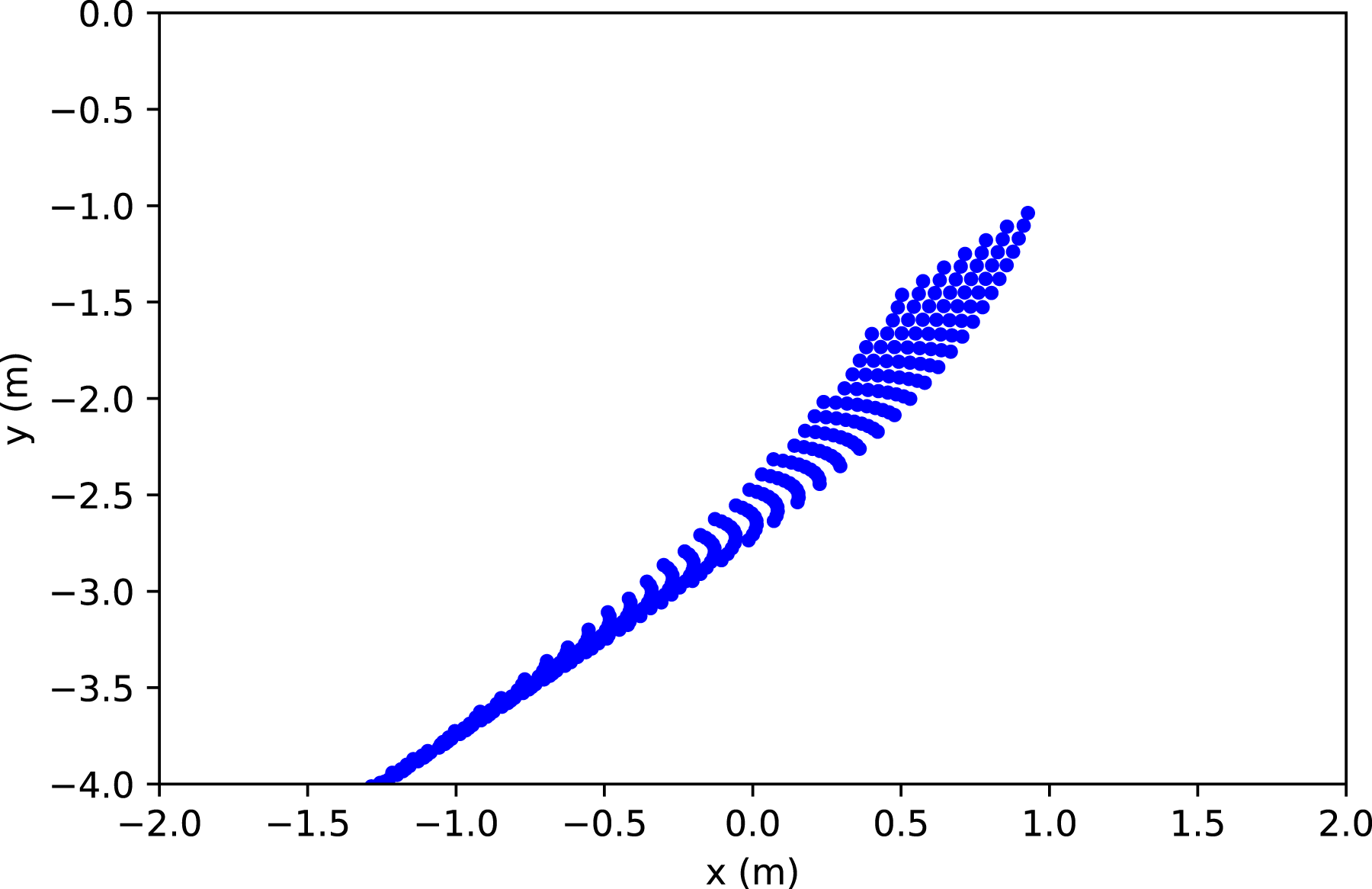
As explained previously, whirls have the structure of “roll-and-catch.” Rolls are R′-circular arcs that finally will be followed by a catch which is a circular arc of
Considering the scenario, the feasibility regions for the starting points of the extremals are sketched and the related costs are calculated. In the following subsection, the costs are compared to determine the path with the minimum cost when starting in different parts of the x − y plane in 2D.
4.4. Map of the optimal paths
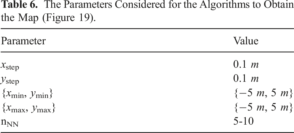
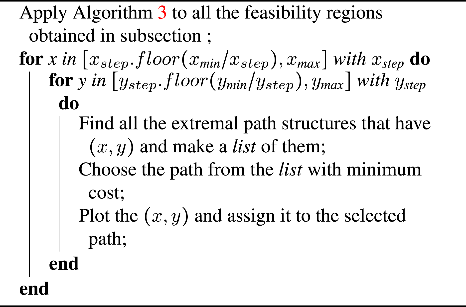
The subsequent process for the considered scenario is followed to compare the costs and draw the map (Figure 19) of the optimal paths: • The parameters reported in Table 6 are considered for the scenario (that was introduced in subsection of Particular Scenario and Steps to Find the Optimal Paths). • Algorithm 3 is applied to all the obtained feasibility regions. To compare the costs of extremal path structures, they should have the same (x, y) for the samples/grids. Thus, Algorithm 3 is required to create those samples/grids by using the data of the existing samples in the feasibility region of each path. • Algorithm 4 is applied to the data produced in the previous step. Therefore, the minimum-cost path for each (x, y) is chosen and plotted in Figure 19. Map indicating the optimal paths to the origin when starting at different The Parameters Considered for the Algorithms to Obtain the Map (Figure 19).
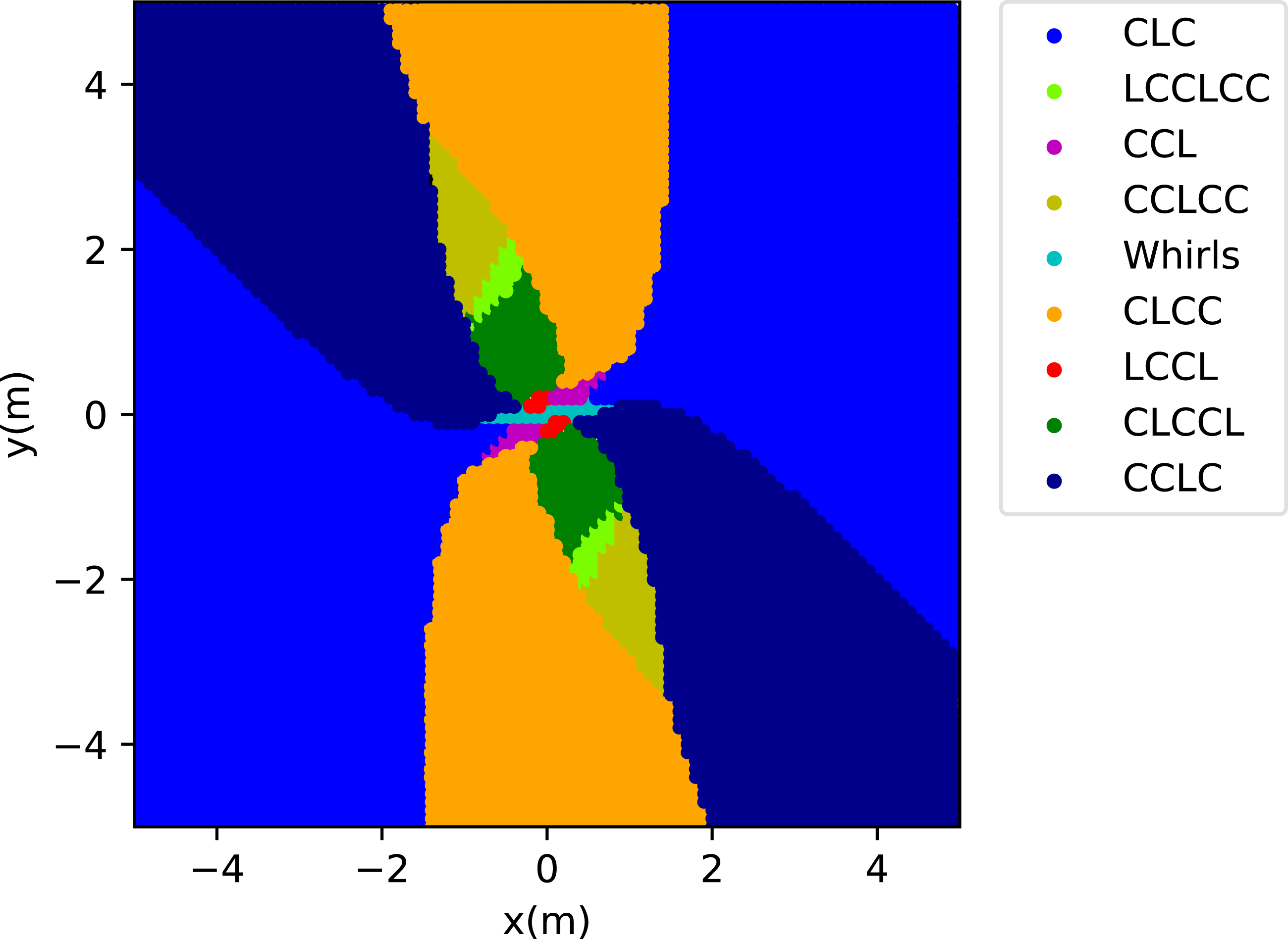
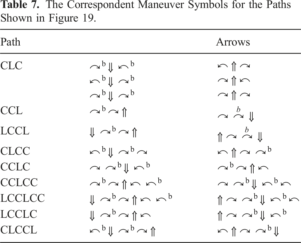
The Correspondent Maneuver Symbols for the Paths Shown in Figure 19.
The paths related to the true blue region (CLC) in Figure 19.
Whirls have the structure of “roll-and-catch”: R′-circular arcs, starting from the initial pose, eventually followed by a turn with • Whirls that are closest to the origin just consist of a catch part. • The other whirls which are far enough from the origin include a roll (a circular arc with R′) and a catch part.
4.4.1. More discussion on the map
Since there are some similarities between the dynamics of differential drive rovers and skid-steer rovers, and also Balkcom and Mason (2002) analyzed a scenario for differential drive rovers similar to ours listed in Table 5 for skid-steer rovers, we discuss similarities and differences between the results in our map (Figure 19) and in Figure 12 presented by Balkcom and Mason (2002). In both figures, there is a type of path which is dominant (covers the most region): PLP for differential drive and CLC for skid-steer rovers. Also, the comparison reveals that instead of R′-circular arcs (“C”), differential drive rovers do point turns (“P”). The analogy extends to either single or pairs of “C”s standing in for “P”s. For example, from similar starting regions, instead of Line-Point turn-Line (LPL) for differential drive, the skid-steer rovers perform LCCL. Also, instead of PLPL for differential drive rovers, skid-steer rovers do CLCCL.
4.4.2. Expectation/Prediction about other scenarios
We expect that for other scenarios beyond the one that was thoroughly analyzed above, the CLC paths will be dominant in the correspondent optimal map. The reason is that avoiding extra turns and instead doing straight lines will normally result in more efficient paths. Therefore, for those regions where CLC paths are feasible, they are the most efficient path. Such CLC paths are generally feasible when the starting pose is far enough from the goal pose, and the goal pose is roughly ahead or behind the start pose. When the goal pose is predominantly to the rover’s left or right, an additional turn (for a CLCC or CCLC) is required. All other path types are only optimal when start and end points are close together, within a few multiples of R′.
The procedure of finding the optimal map involves conducting the grid-producing process, constructing an extremal path structure, and subsequently comparing the costs to derive the optimal map for any starting angle starting (x,y) with the specific angle directed towards the origin. Following this, the look-up table approach can be employed to determine the appropriate path for the specific starting pose. In cases where the entire map creation is unnecessary, applying algorithms 1–4 solely for the selected (x, y, θ) will suffice. In conclusion, two approaches are presented. The first approach entails creating a comprehensive map for various starting angles and employing the look-up table or regression for intermediate specifications. On the other hand, the second approach does not utilize the optimal map or regression and instead follows the explained method of using algorithms 1–4 to obtain the path for a specific pose.
In addition, to illustrate various instances of the predominant paths within the optimal map, Figure 21 is included. Dominant paths on the optimal map. Whirls consist of a roll, that is circular arc with R = R′, and a catch, a circular arc with a tighter R ∈ [0, R′] that puts the rover in the final pose. Green arrow indicates starting pose and red arrow indicates final pose.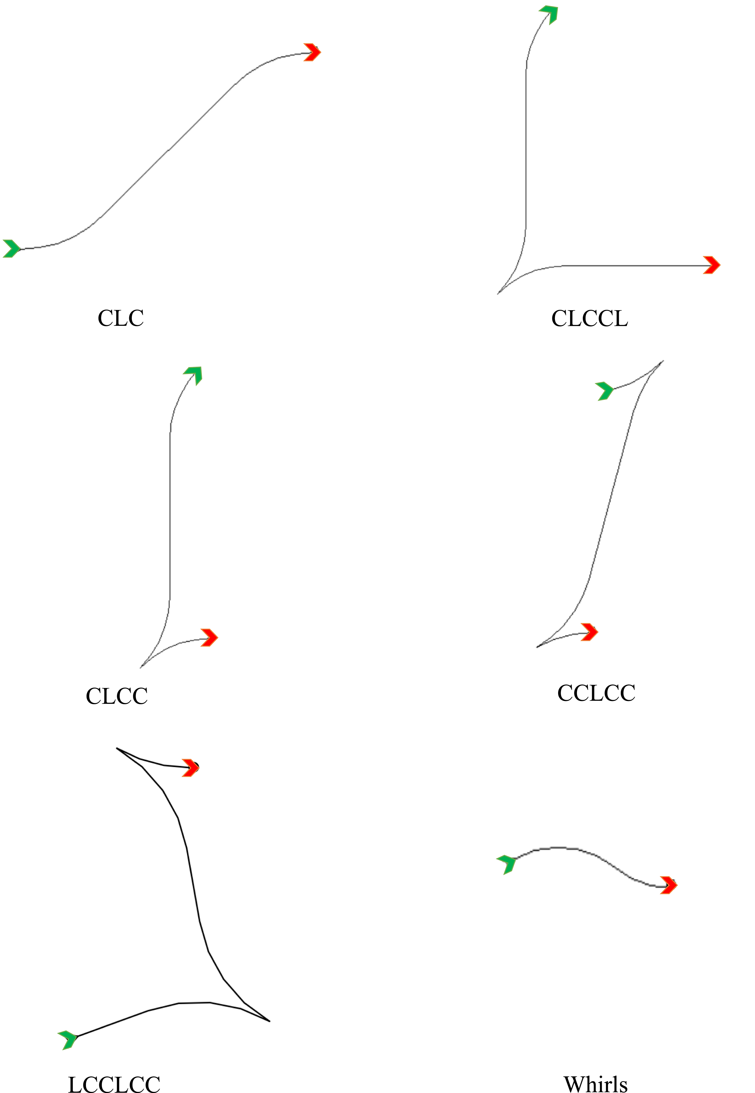
5. Experimental tests
The objective of the work in this section is to provide experimental support for Theorem 1. Specifically, we demonstrate that the following problems have the same optimal answer: (a) (b) The hexagonal control space considered for the Equivalent Time-Optimal experiments.
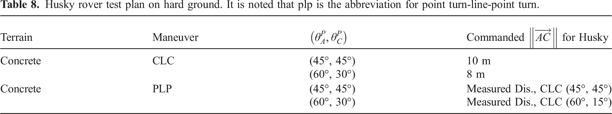
Husky rover test plan on hard ground. It is noted that plp is the abbreviation for point turn-line-point turn.
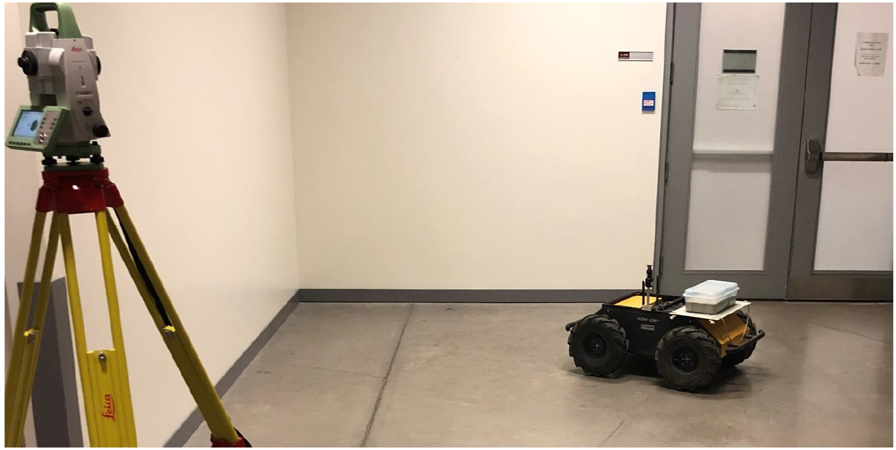
Husky UGV and the laser total station for tracking the rover motion.
The power measurement process encompassed both the left and right motors, employing a Texas Instruments INA226 bidirectional current and power sensor. The power consumption over a specific duration was collected, and then numerically integrated over the time period to determine energy consumption.
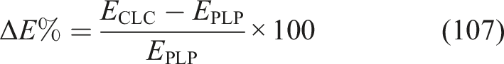
As it can been seen from Figures 24 and 25, the minimum-energy for CLC paths subject to the Constant vc constraint happens at R′ (Effati et al. 2020). Moreover, Figures 26 and 27 show that the minimum time for the equivalent time-optimal problem also occurs at R′. It is noted that the tests are repeated at least 3 times for each turning radius. Energy comparison between CLC and PLP paths for the Constant vc experiments for the distance of 10 m and Energy comparison between CLC and PLP paths for the Constant vc experiments for the distance of 8 m and Time comparison between CLC and PLP paths for the Equivalent Time-Optimal experiments for the distance of 10 m and Time comparison between CLC and PLP paths for the Equivalent Time-Optimal experiments for the distance of 8 m and 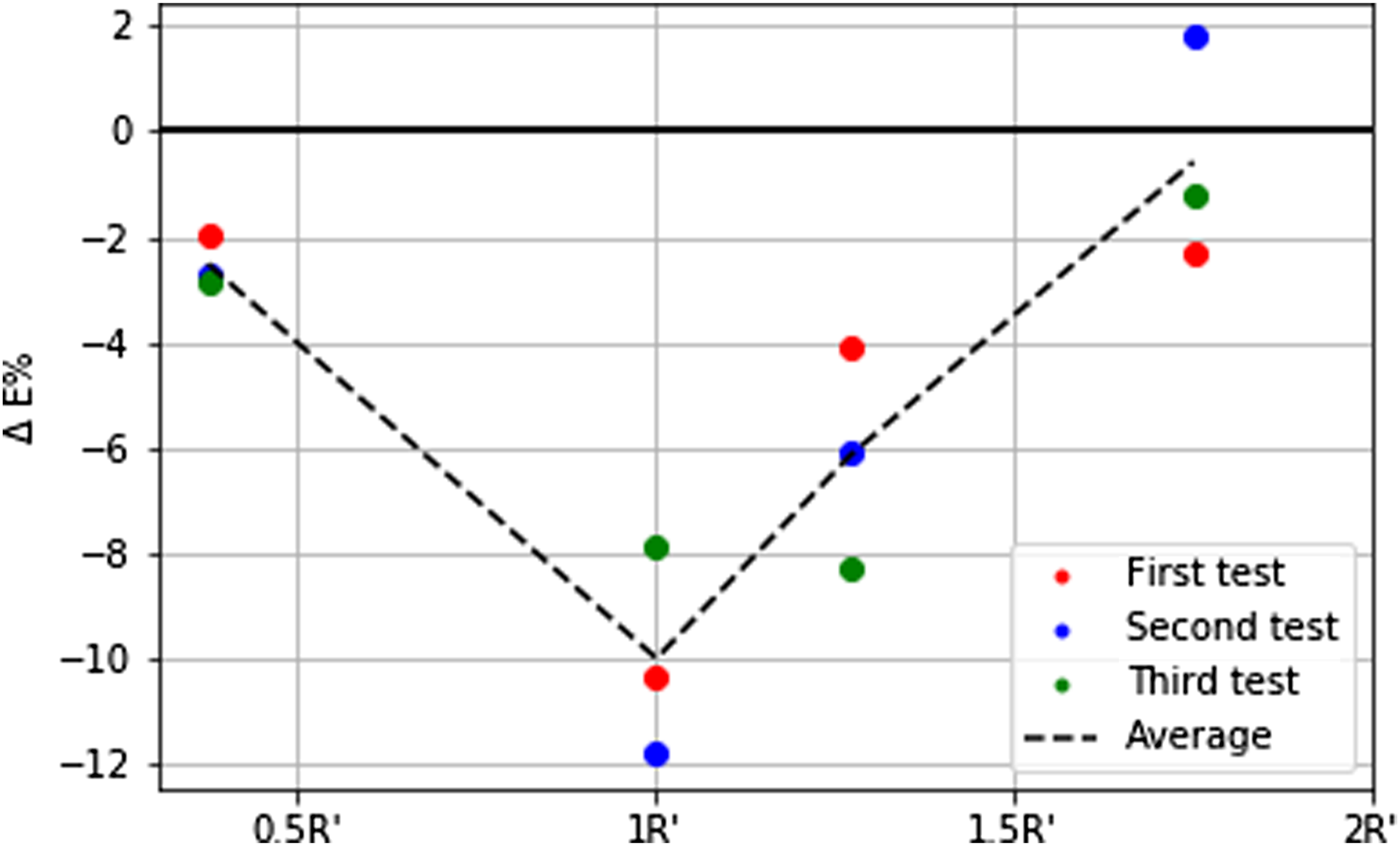
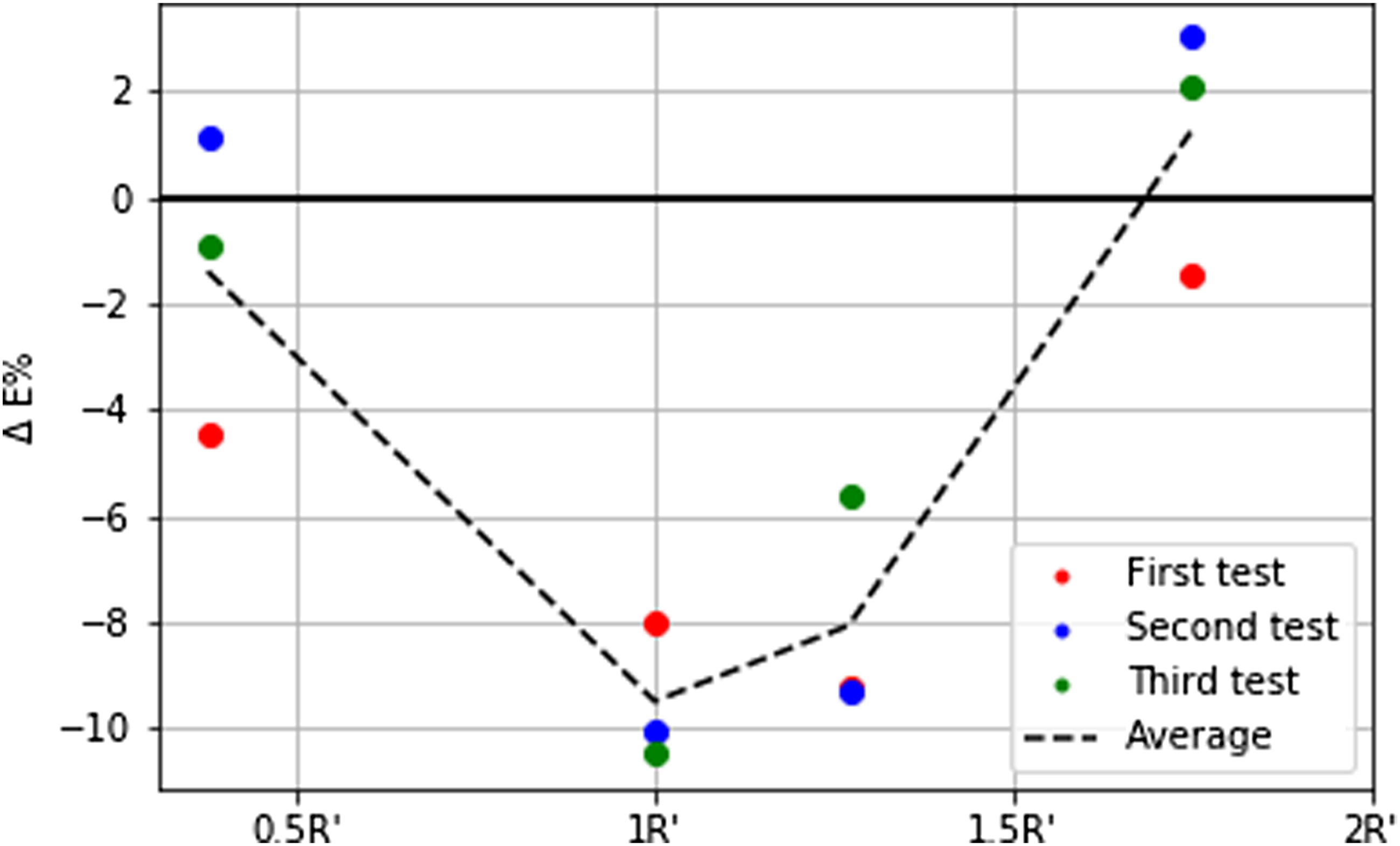
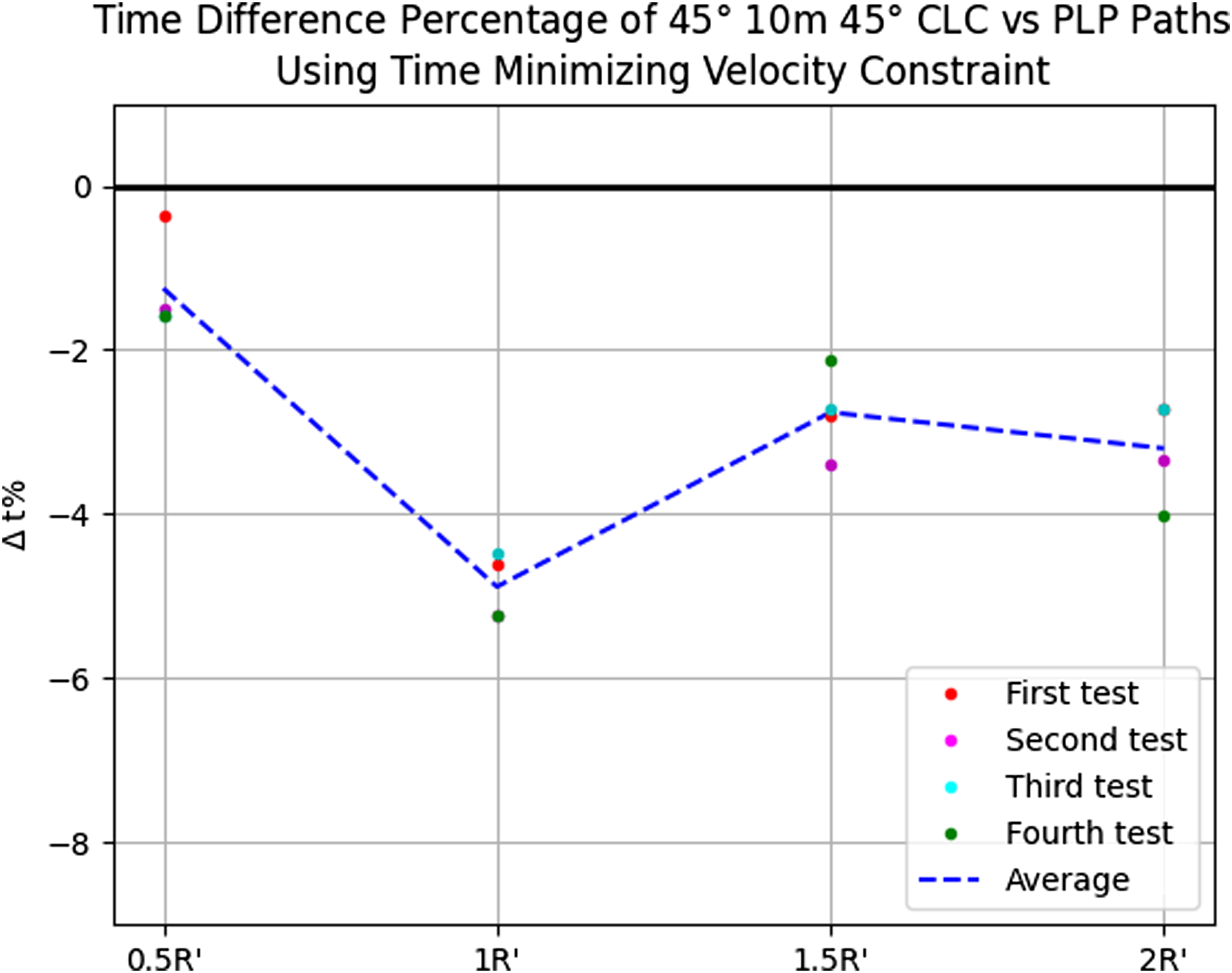
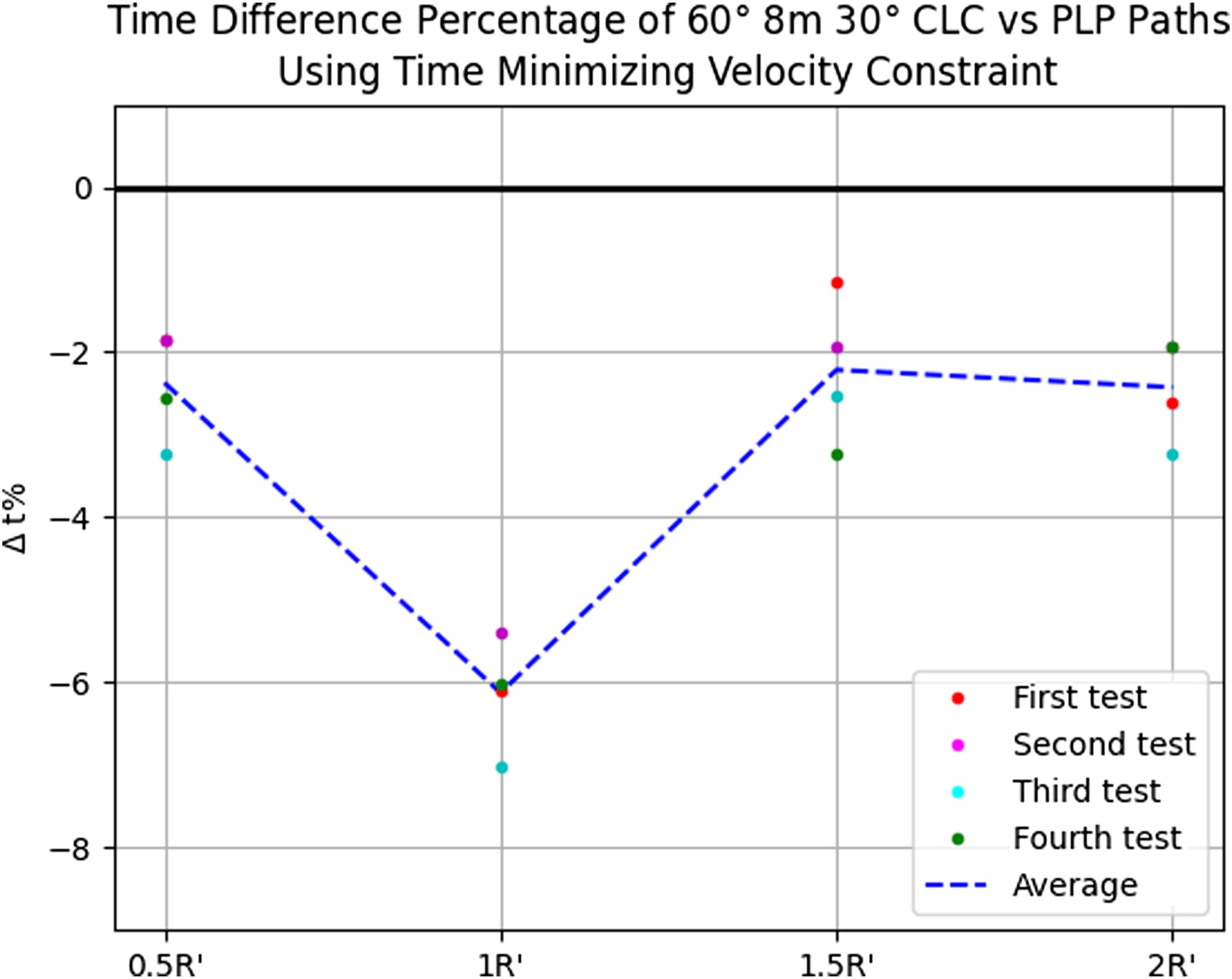
These results provide strong experimental support for Theorem 1, which states that the minimum time optimization problem subject to the hexagonal shape control space (i.e., the constant-power constraint, Figure 14) has the same solution as the minimum energy optimization problem subject to any proper constraint, including the Constant vc constraint.
Measured Energy (ME), Predicted Energy (PE), and the % Error, for Different Turning Radii, for the Distance of 10 m and
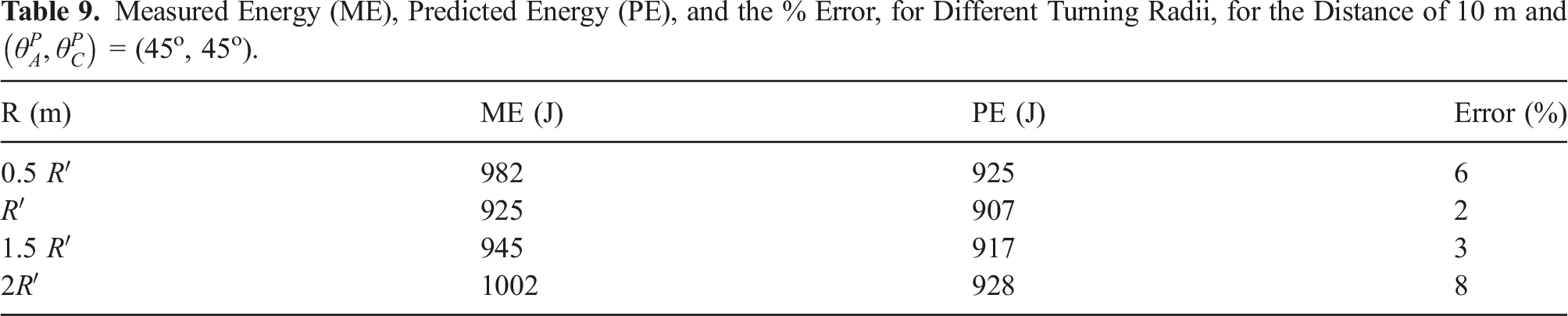
Figure 28 shows a visualization of the paths generated at different R′ values. CLC paths for different turning radii of 0.5 R′, 1R′, 1.5 R′, and 2R′. (a) CLC paths for different turning radii, the distance of 10 meters, and 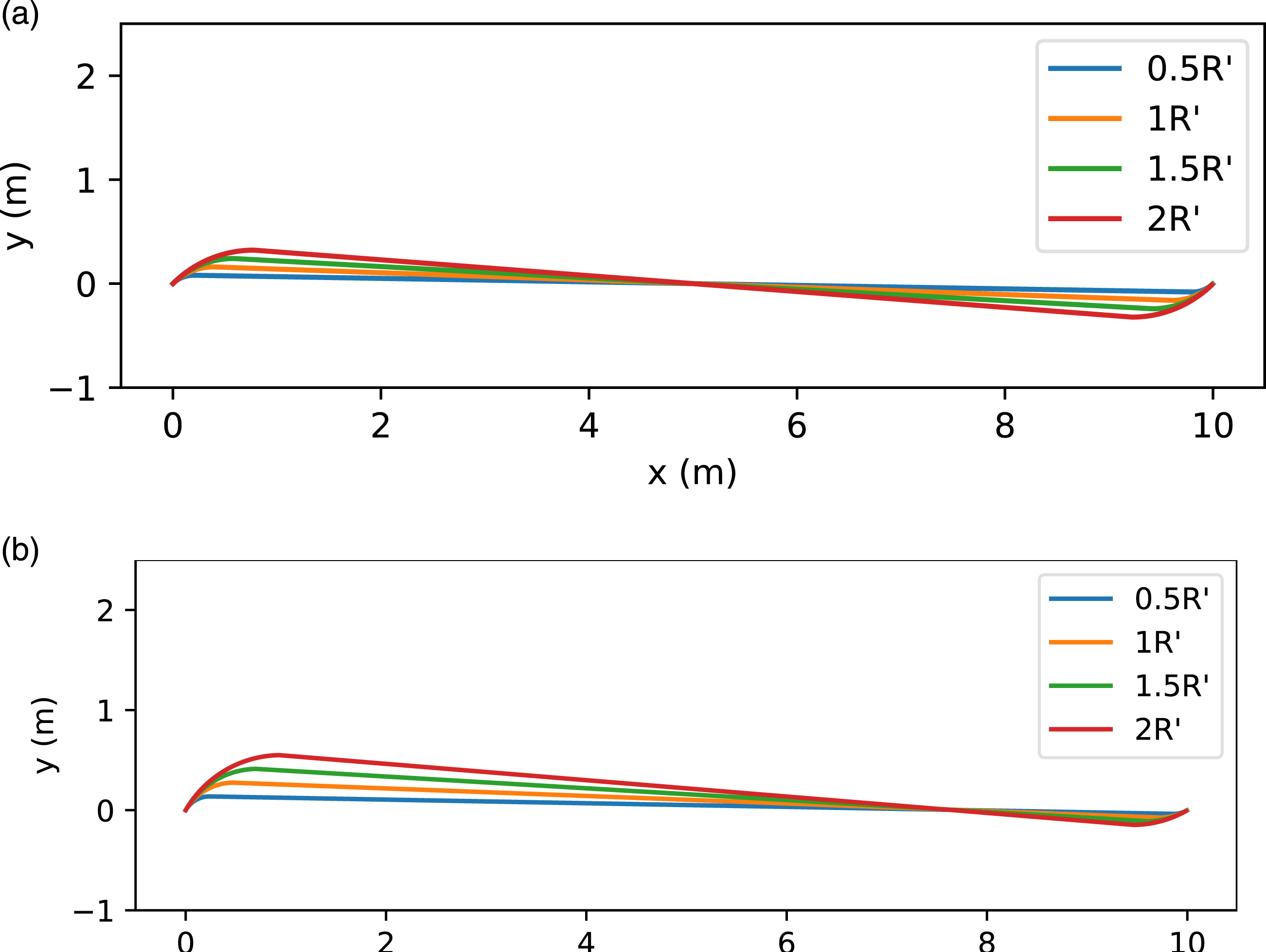
Representative samples comparing the commanded and measured paths from experimental tests are shown in Figure 29. Comparison of commanded and measured CLC paths, with turning radii of 0.5 R′ in this sample. The slight difference between the measured and commanded paths in (b) is due to some excess skidding that occurred toward the end of the path. (a) Commanded and measured CLC paths for the distance of 10 meters and 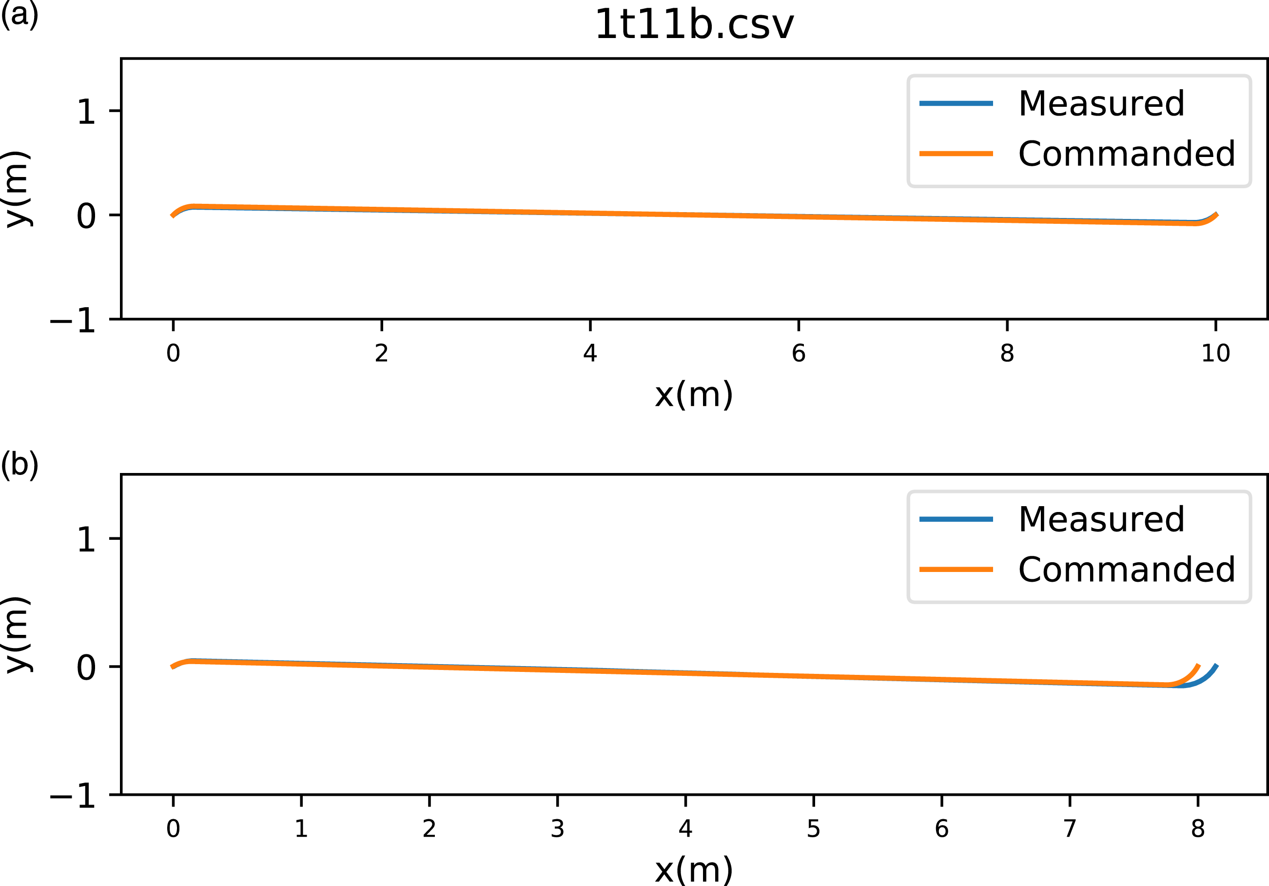
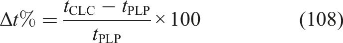
As depicted in Table 8, two distinct scenarios are presented: one involving an angle of (45, 45) degrees and a distance of 10 m, and the other featuring an angle of (60, 30) degrees and a distance of 8 m. Each of these scenarios was evaluated across four varying turning radii (0.5R′, R′, 1.5R′, and 2R′). The energy consumption was calculated for each combination, and subsequently, the average energy consumption was computed. For the first scenario, the average energy consumption attributed to the angular velocity (ω z ) term and the linear velocity (v) are determined to be 31% and 69%, respectively. For the second scenario, the corresponding percentages are 37% and 63%, respectively.
6. Conclusions and future work
The contributions and results of this paper are discussed and summarized here, and then proposed/planned future work is reported.
6.1. Conclusions
Skid-steer rovers consume a lot more power in point turns compared to straight-line motions. As energy is the integral of power over time, lower instantaneous power consumption for wider arcs must be traded off against shorter traversal distance for tighter arcs. A thorough review of the published literature reveals a lack of analytical energy-optimal path planning approaches for skid-steer rovers. This paper has addressed this problem for such rovers moving on obstacle-free hard ground. From the evaluations and investigations of the problem, the following findings are concluded: • • • •
6.2. Future work
Since the power model (equation (22)) is designed for hard ground, all the theoretical analysis in this paper are performed by the assumption of moving on hard ground. However, for applications such as space robotics the rover should be able to follow the optimal trajectory on loose soil. Accordingly, the power model (equation (22)) should be revised for loose soil. Some preliminary research has been performed to identify the power model for loose soil around R′ by Fiset (2019); Fiset et al. (2019). However, it still requires more investigation to obtain a proper power model on loose soil. After the mentioned step, the energy-optimal path planning problem should be solved for this type of terrain.
As both energy and time can be considered in optimal trajectory planning, an interesting direction of future work is optimal path planning by minimizing a hybrid time-energy cost for skid-steer rovers. This may even be directly interesting to energy minimization as, beyond the large share of power used for locomotion, rovers typically also have some component of energy consumption that is approximately constant in time such as electrical power draw for computing and sensing.
Another interesting direction for future work is considering obstacles. As mentioned in the introduction, the scope of this work has been local planning methods (LPM) for the space between nodes that are already chosen to avoid obstacles in a complex environment. However, direct extensions to environments with obstacles might prove fruitful, especially if the obstacles are sparse. In that case, initial LPM solutions could be checked for obstacle intersection, with interim nodes iteratively added in case of intersections; adaptive processes for such tasks would need to be developed.
Finally, results from this work could immediately be integrated into ongoing work with skid-steer rovers that use Sampling Based Model Predictive Optimization (SBMPO). Instead of “sampling” from among the space of admissible controls, one could simply use the same six optimal candidate controls (forward, backward, and the 4 R′ turns) at each branching point in the SBMPO framework and obtain results closer to the global optimum at lower computational cost.
Footnotes
Acknowledgements
The authors acknowledge funding and technical collaboration from Mission Control Space Services Inc. as well as financial support from the Natural Sciences and Engineering Research Council of Canada (NSERC). Additionally, the authors acknowledge Tim Freiman’s collaboration in conducting the experiments to generate the two figures related to the time-optimal experiments.
Declaration of conflicting interests
The author(s) declared no potential conflicts of interest with respect to the research, authorship, and/or publication of this article.
Funding
The author(s) disclosed receipt of the following financial support for the research, authorship, and/or publication of this article: This work was supported by the Canadian Network for Research and Innovation in Machining Technology and Natural Sciences and Engineering Research Council of Canada (NSERC CRD 520713-2017).