
Abstract
Soft robots have been investigated for various applications due to their inherently superior deformability and flexibility compared to rigid-link robots. However, these robots struggle to perform tasks that require on-demand stiffness, that is, exerting sufficient forces within allowable deflection. In addition, the soft and compliant materials also introduce large deformation and non-negligible nonlinearity, which makes the stiffness analysis and modelling of soft robots fundamentally challenging. This paper proposes a modelling framework to investigate the underlying stiffness and the equivalent compliance properties of soft robots under different configurations. Firstly, a modelling and analysis methodology is described based on Lie theory. Here, we derive two sets (the piecewise constant curvature and Cosserat rod model) of compliance models. Furthermore, the methodology can accommodate the nonlinear responses (e.g., bending angles) resulting from elongation of robots. Using this proposed methodology, the general Cartesian stiffness or compliance matrix can be derived and used for configuration-dependent stiffness analysis. The proposed framework is then instantiated and implemented on fluidic-driven soft continuum robots. The efficacy and modelling accuracy of the proposed methodology are validated using both simulations and experiments.
1. Introduction
The field of robotics has experienced a paradigm shift from traditional robots, made of rigid links and joints, to soft robotic structures (Laschi et al., 2016). Soft robots often distinguish themselves from traditional robots by their intrinsic dexterity, biological morphology, and adaptability to unstructured environments (Shepherd et al., 2011; Arezzo et al., 2017; Rus and Tolley 2015). These versatile capabilities can be (in)directly credited to the compliant properties of the soft materials used to construct the robots. Soft robots have been investigated for safety-related applications in the industrial sector where robots work closely together with humans (Stilli et al., 2017), in minimally invasive interventions (Cianchetti et al., 2014; Abidi et al., 2018), and rehabilitation (Camp et al., 2021).
The stiffness (or its inverse, i.e., the compliance) of a soft robot can be mathematically described by the Young’s modulus defined as the relationship between an applied load and its corresponding deflection. The term soft robot fundamentally implies that the Young’s modulus of such a robot is a few orders less than 109 − 1010 Pa, a Young’s modulus range for conventional robotic materials such as metals and hard plastics (Majidi 2014). Soft robots, however, are made of materials with a Young’s modulus of approximately 104 − 106 Pa, and they behave in a compliant way when in physical interaction with the environment. As a result, it might be challenging for soft robots to exert sufficient forces on demand. Hence, the investigation of stiffness property and stiffness adjustment is profoundly important to the design, modelling and control of soft robots (Mahvash and Dupont 2011; Naselli and Mazzolai 2021; Komatsu et al., 2021).
1.1. Related work
A number of stiffening mechanisms have been investigated to vary compliance of soft robots. These can be categorised into semi-active techniques, such as actuators that can change their Young’s modulus, and active actuators (Manti et al., 2016). Techniques for achieving stiffness variation in semi-active and active ways include the integration of granular material (Konstantinova et al., 2022), use of an alloy with a low melting point (Peters et al., 2019), and the combination of tendon-driven and air pressurisation through antagonistic actuation (Shiva et al., 2016). Researchers have highlighted challenges in embedding these stiffness mechanisms in soft manipulators for space-restricted applications, such as minimally invasive surgery (Runciman et al., 2019). Apart from the aforementioned mechanism design, the stiffness characterisation is advantageous for understanding the payload capability of the soft robots. An experimental-based stiffness assessment is presented by Ranzani et al. (2016), characterising the planar stiffness of a single pneumatic-driven modular manipulator. A similar approach is followed by Mustaza et al. (2018), where the spatial compliance ellipsoid was experimentally identified.
Once the stiffness properties of soft robots are comprehended, the subsequent stage is to formulate their statics or dynamics models. Various beam theories, such as the Euler–Bernoulli beam theory (Stilli et al., 2018) and the Timoshenko beam (Lindenroth et al., 2016), have been investigated to establish the forward kinematics of soft robotic manipulators. The utilisation of the Euler–Bernoulli beam theory has also demonstrated that the flexural rigidity of tendon-driven robots is subject to variation based on tendon stiffness, thus influencing robot kinematics (Oliver-Butler et al. 2019). The Piecewise Constant Curvature (PCC) model is a well-known method for statics and dynamics modelling of soft robots (Webster and Jones 2010; Caasenbrood et al., 2023). This model assumes that the curvature along the robot’s length is constant. When calculating the resulting strains from applied moment and torque, the PCC model requires consideration of bending and elongation stiffness (Sadati et al., 2017). Common variable curvature models include the Cosserat/Kirchhoff rod theory (Renda et al., 2018; Grazioso et al., 2019). A geometrically exact Cosserat model was proposed in Trivedi et al. (2008) to describe the forward kinematics of multi-segment continuum robots, considering material nonlinearities. Based on the Cosserat rod theory, the forward kinematics are modelled for a three-segment tendon-driven continuum robot with extensible sections (Amanov et al., 2021). Furthermore, a real-time dynamics modelling framework, based on the dynamic Cosserat rod equations, is applied to a tendon-driven continuum robot, parallel robot, and fluidic-driven soft robot (Till et al. 2019). In addition, a Cosserat model-based method is proposed for a pneumatic-driven continuum robot with braided chambers to then further sense environmental stiffness in real-time (Sadati et al., 2020). A new discretised model and a Matlab package (TMTDyn) was then presented for hybrid rigid-continuum systems based on Euler–Bernoulli beam and Cosserat rod model (Sadati et al., 2021). Based on the material properties, numerical analysis can be conducted, for example, using Finite Element Modelling (Elsayed et al., 2014; Koehler et al., 2019; Zupan and Saje 2003). In summary, the aforementioned modelling techniques are built on known stiffness properties of robots. The material properties (e.g., Young’s modulus), together with bending, elongation and shear stiffness, are usually considered to calculate curvatures and strains from actuation forces. The resulting curvatures and strains complete the statics or dynamics models. However, a thorough stiffness description and analysis for soft robots, for example, the Cartesian stiffness, is not investigated in these models.
The importance of understanding configuration-dependent stiffness has been proven for traditional rigid link and continuum robots (Ajoudani et al. 2015, 2017; Gravagne and Walker 2002; Stella et al., 2023). The difference between stiffness controllability in traditional rigid robots compared with soft robots primarily lies in the generation of compliance. In rigid robots, the compliance is provided by finite variable stiffness joints (Wolf et al., 2015). The stiffness matrix in Cartesian space is determined based on the Jacobian projection (Salisbury 1980; Alici and Shirinzadeh 2005). Instead, many soft robots are considered continuum manipulators without physical joints; the compliance is distributed along the robots (Naselli and Mazzolai 2021). A pioneer work for compliance analysis of continuum robots is to use ellipsoid analysis (Gravagne and Walker 2002), analogous to the techniques used in the rigid-link robots. The stiffness properties of soft robots can be characterised by discretising their structures into finite elements with a diagonal stiffness matrix, using the Cosserat rod model for instance (Renda et al., 2018). With this approach, researchers have proposed a Cartesian impedance control method for planar soft robots composed of multiple segments, assuming a PCC model (Della Santina et al., 2020). Moreover, there are efforts towards a detailed analysis of passive stiffness in soft robots, such as the development of an augmented Jacobian-based method using Ordinary Differential Equations (ODEs) to obtain the compliance matrix (Rucker et al., 2011), and the establishment of statics models based on the Cosserat rod theory. Such a concept was then adopted and developed by Black et al. (2017) to analyse the stiffness response of a parallel continuum robot under different configurations. Inspired by the work of Rucker et al. (2011), a new set of compliance differential equations was developed, directly coupled to the solution of the forward kinematics. These equations were employed to derive the compliance matrix of continuum robots (Smoljkic et al., 2014). However, the robotic manipulators were approximated to the slender Kirchhoff rod, whilst large elongation observed in soft robots was not considered (Gong et al., 2021; Caasenbrood et al., 2023).
As for the specific mathematical tool for the compliance modelling in robotic field, Lie theory (Sonneville et al., 2014) and, in particular, screw theory have been utilised in robotics for it concisely interprets rigid-body motions, such as kinematics and statics modelling (Renda et al., 2017), parameter calibration (Sun et al., 2020; Cibicik and Egeland 2021) and identification (Fu et al. 2020), and compliance analysis (Qi et al., 2016; Selig and Ding 2001; Ding and Dai 2010). In addition, an analytical model was presented in Hussain et al. (2021) to model and analyse the stiffness ellipsoids for a tendon-driven soft-rigid gripper.
1.2. Problem statement and motivation
Summary of soft robotic modelling and stiffness/compliance analysis.
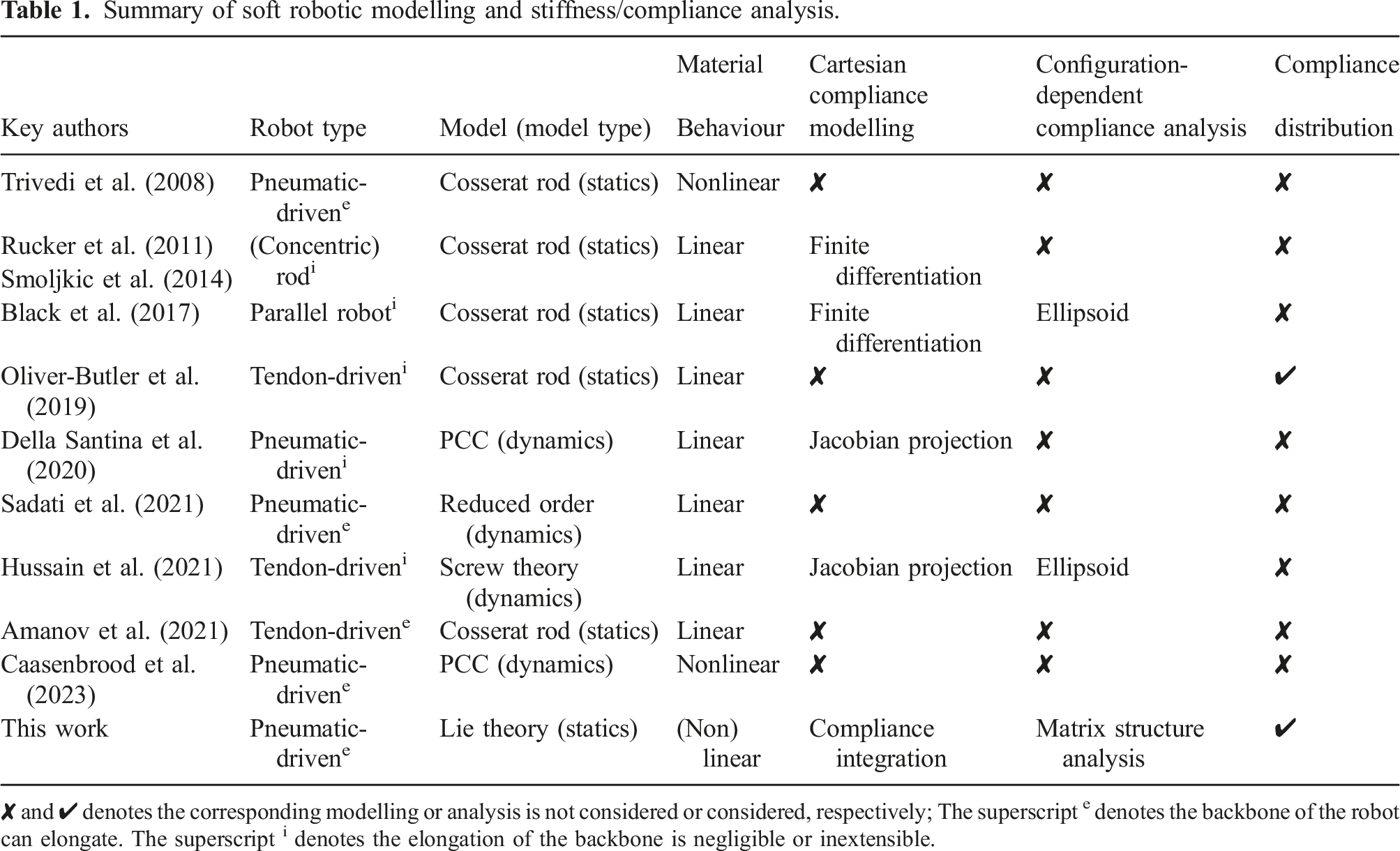
✘ and ✔ denotes the corresponding modelling or analysis is not considered or considered, respectively; The superscript e denotes the backbone of the robot can elongate. The superscript i denotes the elongation of the backbone is negligible or inextensible.
As such, a systematical modelling approach and analysis of configuration-dependent stiffness and compliance distribution remain challenging. Moreover, for elastomer-based soft robots, the elongation of the robots’ backbone often reduces the cross-sectional area. This behaviour introduces nonlinearities and also influences stiffness properties of these robots. Motivated by the aforementioned considerations, a stiffness modelling and analysis framework should make an important contribution to the soft robotics community.
1.3. Contributions and outline
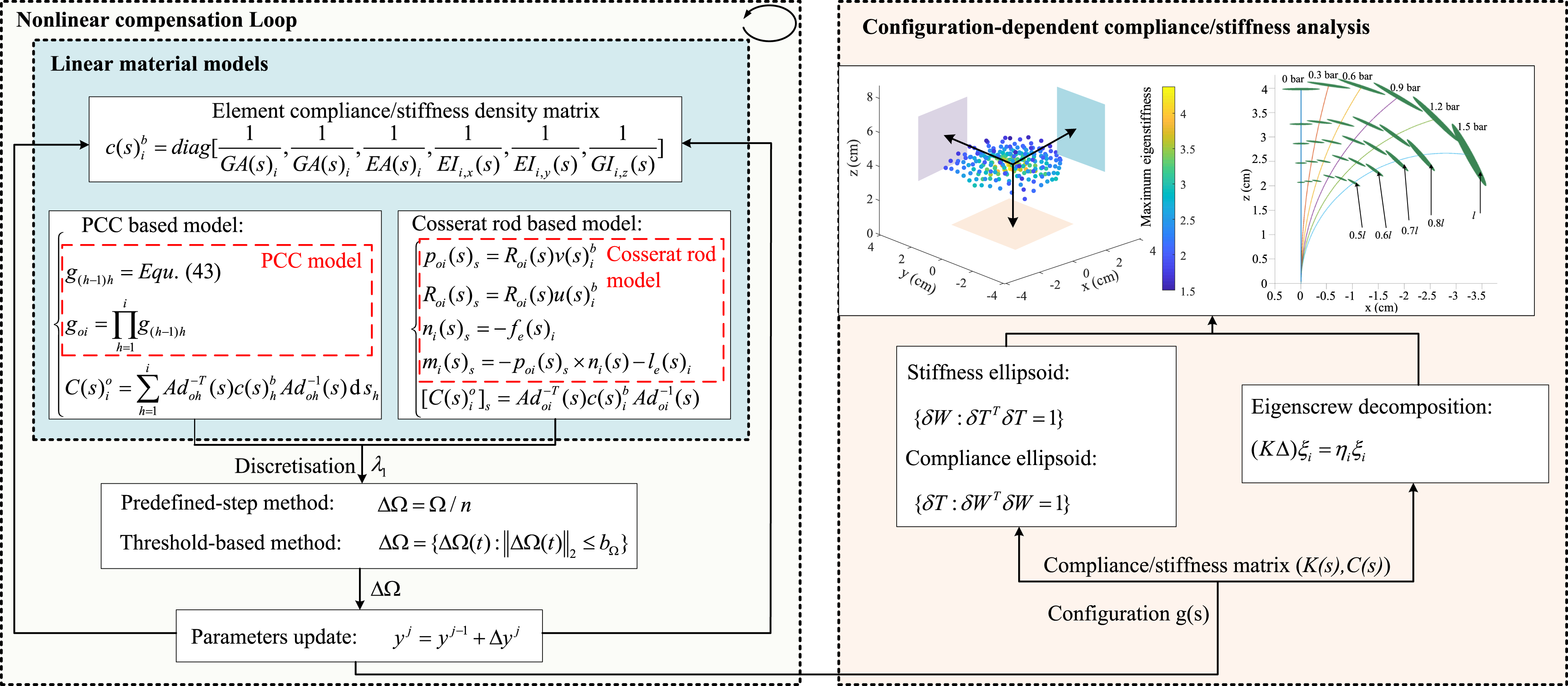
In our previous work (Shi et al., 2021), we proposed a Cartesian stiffness modelling method based on the PCC model for a single fluidic-driven soft robot. The paper included preliminary validation data on the tip stiffness. Going beyond our previous work, this paper proposes a Lie theory–based stiffness modelling and analysis framework for soft fluidic-driven robotic manipulators to investigate their underlying stiffness characteristics and deliver a configuration-dependent stiffness/compliance analysis. Our framework, illustrated in Figure 1, incorporates forward kinematics and stiffness modelling, considering the nonlinearity introduced by the elongation. Hence, the linear and nonlinear material behaviours are explored, embedded in the PCC model and the Cosserat rod model. To validate our framework, we apply it to a single soft fluidic-driven robotic manipulator and a manipulator composed of two segments. This work provides an approach to analyse the general stiffness based on the commonly used static kinematics models. In particular, the contributions made by this work are Table 2: 1. Our proposed Lie theory–based modelling framework (see Section 2) is capable of configuration-dependent stiffness modelling and analysis at different static robot configurations from forward kinematics models (e.g., the PCC and Cosserat rod models). This framework considers nonlinear responses resulting from large longitudinal deformations (e.g., when elongating or bending) as presented in Sections 2.3 and validated in Sections 5.2. 2. Our methodology demonstrates that the robot compliance can be derived by various integration schemes based on the obtained static configurations of soft robots, without using Jacobian projections or finite differentiation (see Section 2.1). We showcase that our approach allows deriving the compliance matrix by direction integration with forward kinematics models, for example, the proposed Cosserat rod-based compliance model (see Section 2.2.2). 3. Our modelling framework can thoroughly reveal the compliance distribution, and for the first time, we achieve a detailed configuration-dependent compliance/stiffness modelling and analysis for extensible fluidic-driven continuum robots (see Section 3 and Section 4). In Section 5, we validate computational results compared to experiments, using soft manipulators made of one and two robotic segments. Diagram of the proposed Lie theory–based framework incorporating forward kinematics, stiffness modelling and analysis. This stiffness modelling and analysis framework accommodates the nonlinear behaviours of kinematics, exemplified by the piecewise constant curvature (PCC) model and the Cosserat rod model, and achieves a configuration-dependent stiffness analysis. Parameters and notations.
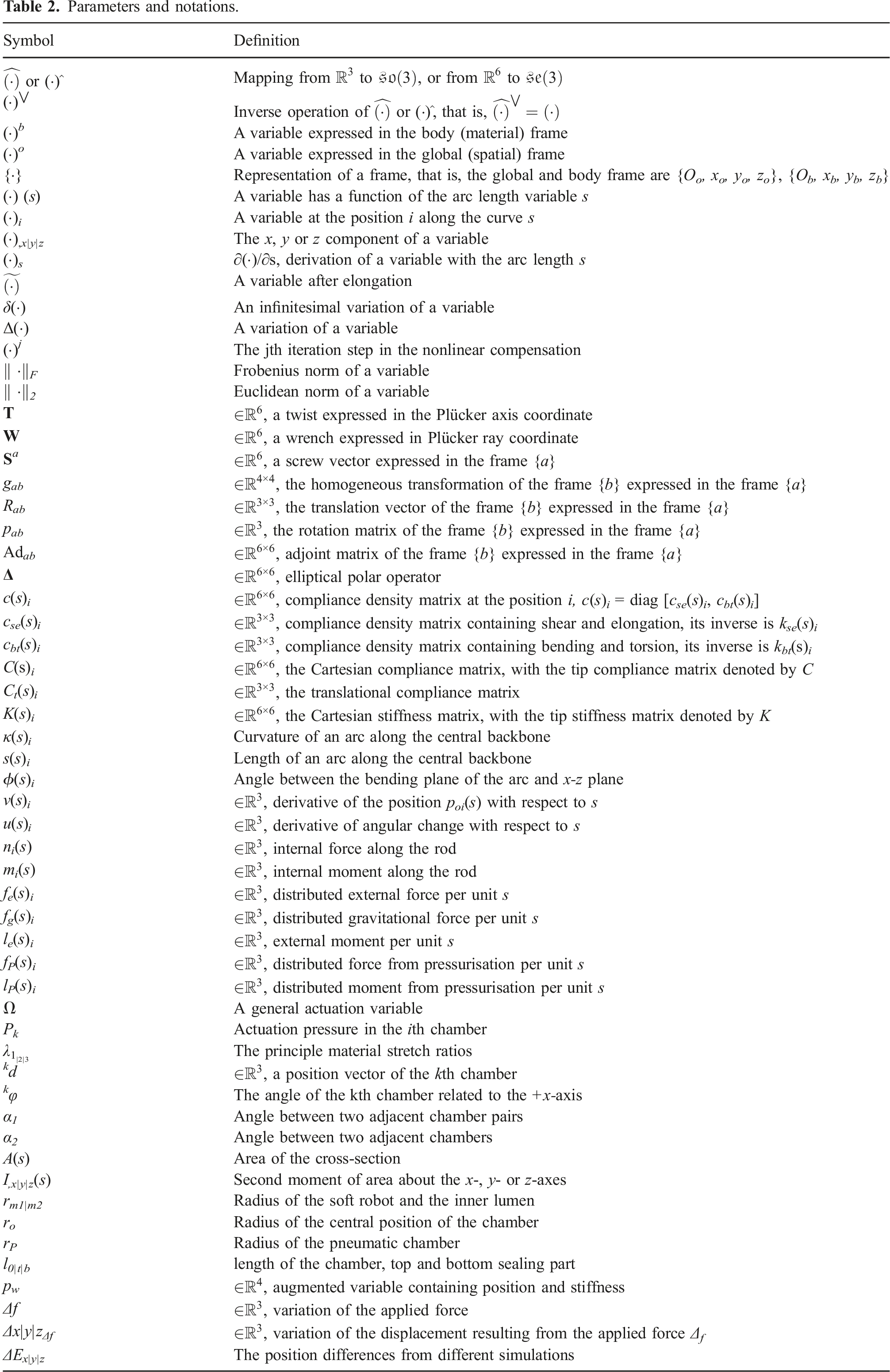
The remainder of this paper is organised as follows: Section 2 proposes the stiffness modelling framework and elaborates its derivations. Section 3 presents the instantiation of the proposed framework based on pneumatic-driven soft continuum robots. The simulation and model-based stiffness analysis are discussed in Section 4. The experimental validation is then presented in Section 5 to demonstrate the efficacy and explore the accuracy of the proposed framework. Finally, the corresponding discussions and conclusions are presented in Section 6.
2. Theoretical framework of the stiffness modelling and analysis
In line with Figure 1, this section presents the stiffness modelling and analysis framework in detail. Compliance matrices are first formulated using Lie theory based on screws. The configuration-dependent Cartesian compliance is built on the PCC and Cosserat models. This is the fundamental difference compared to current approaches that focus on forward kinematics only (see the dotted red rectangle in Figure 1). Furthermore, our proposed framework considers nonlinear responses resulting from large longitudinal deformations of the incompressible material during elongation and bending. The output of the proposed framework includes the forward kinematics and the general stiffness/compliance matrix, resulting in a configuration-dependent stiffness modelling and analysis.
2.1. Cartesian compliance matrix derivation
The basics of screws and Lie theory are summarised in Appendix B. In general, the relationship between a twist 
C is the 6 × 6 compliance matrix, and K is the 6 × 6 stiffness matrix with the relationship C = K−1. C and K are interchangeable and both used in this paper.
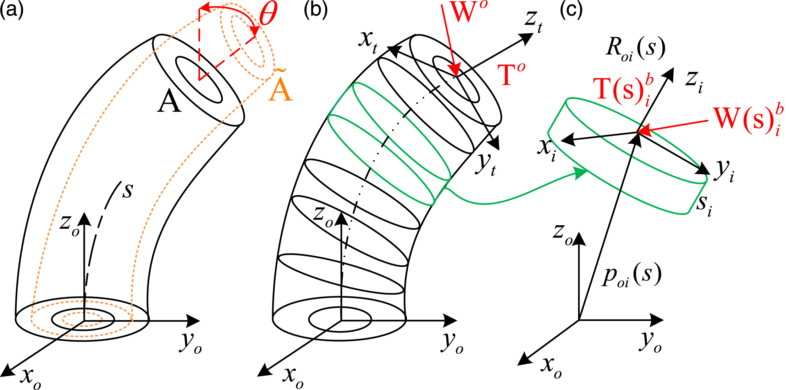
The soft continuum robot can be discretised into finite elements. So in this paper, we use i to denote the ith discretised element and s to denote the continuous curve along the backbone (see Figure 2). The material compliance density Illustration of the deformed robot with a bending angle θ (when the cross-section is circular). (a) The variation of the cross-section is non-negligible under a large longitudinal deformation for the incompressibility of the material. (b) The soft manipulator comprises serially connected compliant elements. (c) An element of the manipulator.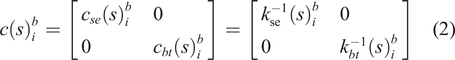
The material compliance density written in the global frame 
From Figure 2(b), the whole manipulator is regarded as the combination of flexible elements (Qiu and Dai 2021; Qi et al., 2016). When a wrench 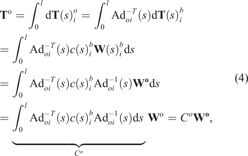
Equation (4) represents the general integration form of the Cartesian compliance based on static robot configurations, illustrating that the compliance is configuration-dependent. Various numerical integration schemes can achieve the compliance integration of (4), once the static configurations of robots are obtained from the forward kinematics. For instance, the midpoint or trapezoidal integration schemes could be applied. In this case, the total Cartesian compliance 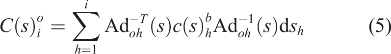
The number of i is the discrete element numbers. In Section 2.2.1, we introduce the PCC-based compliance modelling approach, utilising either the midpoint or trapezoidal integration scheme with robot configurations derived from the PCC model. The discrete arc numbers in the PCC model are denoted by i, and high-order integration schemes can also be considered. Additionally, in Section 2.2.2, we present the Cosserat rod-based compliance modelling approach, employing a high-order Runge–Kutta integration scheme. We demonstrate the benefits of performing compliance integration simultaneously with the forward kinematics model in this case.
It is important to note that the selection of the compliance integration scheme is not limited by the statics models. Our approach allows for the exploration of various integration schemes to derive compliance based on the static configurations of robots. Therefore, any integration scheme can be considered and evaluated within our framework.
2.2. Configuration-dependent compliance model
As detailed in Section 2.1, (4) needs to be combined with the forward kinematics models. We complete our modelling framework by proposing the PCC-based and the Cosserat rod-based compliance modelling.
2.2.1. PCC-based compliance model
In the PCC model, the spatial backbone is depicted via a set of serially connected discrete arc whose curvature parameters are [κ(s) i , s(s) i , ϕ(s) i ] of the ith element. κ(s) i is the curvature, s(s) i is the curve length and ϕ(s) i is the angle of the arc that rotates from the x-z plane. Using the exponential mapping from Lie theory, the homogeneous transformation gi(i+1) from ith arc to (i + 1)th arc using screws (Webster and Jones 2010; Shi et al., 2021). The general form of gi(i+1) is shown in (43) (see Appendix C).
Substituting all the arc parameters [κ(s)
i
, s(s)
i
, ϕ(s)
i
] into gi(i+1), the general forward kinematics g
oi
(s) is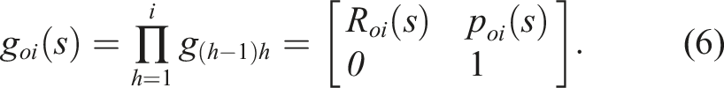
Equation (6) can be used to get the adjoint matrix. The PCC-based compliance modelling is derived by combining (5)–(6). The number of i is the discrete arc numbers in the PCC model and influences the accuracy of the calculated compliance
2.2.2. Cosserat rod-based compliance model
The constant curvature assumption is not needed in the Cosserat rod model. However, the traditional Cosserat model focuses on the statics or dynamics, the compliance/stiffness modelling is not included. A Cosserat rod-based compliance model is proposed in this paper, where the stiffness modelling is directly incorporated, without calculating the static robot configurations in advance.
The mechanics of the rod can then be derived by a set of partial differential equations within the Lie group (Till et al. 2019). By convention, the subscript s means the derivative with arc length s, namely, ∂/∂s. The variable 
The distributed forces and moment along the rod are denoted by f
e
(s)
i
and l
e
(s)
i
, respectively. The classic equilibrium of the Cosseart rod satisfies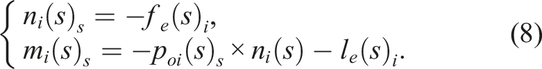
The linear constitutive equation relates u(s)
i
, v(s)
i
to the loading n
i
(s), m
i
(s), and the linear relationship yields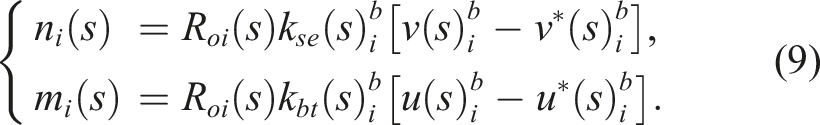
The variables
Recalling (4), the derivative of the compliance matrix, namely the compliance density, can be obtained by
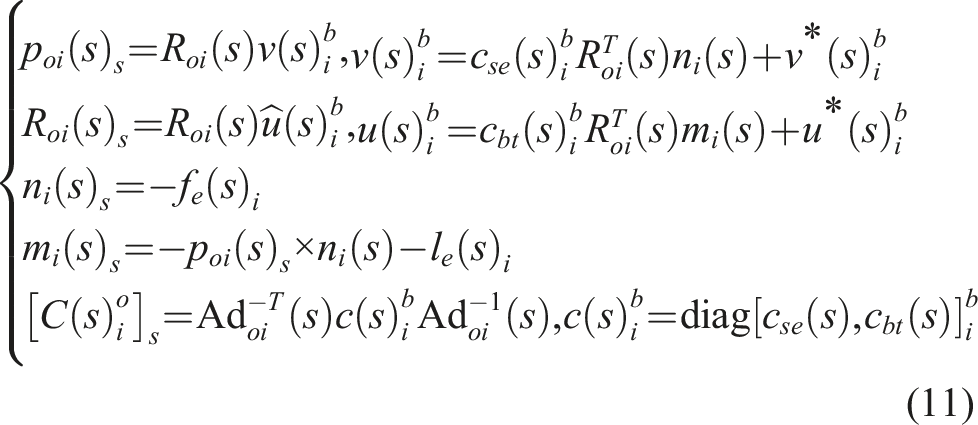
Numerical integration methods, such as a high-order Runge–Kutta approach, can be used to solve (11). It is noteworthy that if the integration truncation error of R oi (s) results in R oi (s) ∉ SO(3), R oi (s) might be represented by quaternion when doing the integration (Rucker 2018). If the initial conditions are known, (11) could be integrated directly as an initial value problem. When the initial states are unknown, (11) can be solved as a boundary value problem using the shooting method (Florian and Damien 2020). Equation (11) gives the analytical representation of the distributed compliance based on the conventional static Cosserat rod equations, where the compliance distribution is not included (Renda et al., 2018; Till et al. 2019). Moreover, the compliance matrix in the proposed Cosserat rod-based compliance model is derived directly without the prerequisite of the Jacobian or finite difference approximations (Rucker et al., 2011; Smoljkic et al., 2014).
2.3. Nonlinear responses compensation
As introduced in Section 2.1, the fluidic-driven robot could have large elongation under high pressurisation (Figure 2(a)). This elongation introduces nonlinear kinematic responses (Gazzola et al., 2018; Caasenbrood et al., 2023). To account for this nonlinearity, we introduce a compensation method in this section, inspired by the nonlinear matrix structural analysis (NMSA) method presented in Naselli and Mazzolai (2021). The NMSA method addresses large deformations in soft bodies by applying load in predefined steps. This method enables the use of a linear strain–stress relation to consider large deformations. Therefore, our proposed framework can generally be applied when an overall strain–stress assumption is less effective, without changing the fundamental models in Section 2.1–2.2, such as the method for constructing the compliance density matrix (see (2)). The load/actuation is applied incrementally, and even with a linear material model, the computation is nonlinear because the system parameters, such as the stiffness matrix density, are updated based on the previous step’s results. The three procedures are:
2.3.1. Procedure 1
The actuation is applied in an incremental way ΔΩ, which is either by predefined n steps or an absolute threshold value bΩ. Using predefined steps, the incremental actuation variable ΔΩ can be described by
Ω is the maximum actuation variable, which could be the fluidic pressure, fluid volume, or external loads in fluidic-driven robots. System parameters update in each step and ΔΩ is used in every step instead of Ω. In the threshold method, ΔΩ equals
Equation (13) denotes that the system parameters update when the variation of the actuation variable in the 2-norm is larger than bΩ. ΔΩ(t) is defined as the variation of Ω after the current update starts, which is reset to zero when the next update step begins. Equation (12) can be used if the maximum value of actuation is known, for example, a step input. By contrast, (13) is more convenient if the actuation changes with time, for instance, a ramp or a sine wave input.
2.3.2. Procedure 2
From (1), the increment of the twist at position i, in the jth step in body frame can be described by

2.3.3. Procedure 3
At the end of the jth step, the compliance matrix density (2) updates based on the results from the (j − 1)th step. When the material stretches, the principle stretches are defined as [λ1, λ2, λ3]. A practical way to update the compliance matrix is treating the material as incompressible (λ1λ2λ3 = 1) and undergoing uniaxial extension. This yields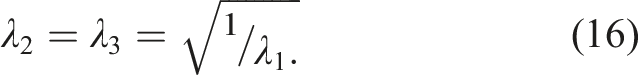
Specifically, when the numerical models including the PCC-based and Cosserat rod-based compliance models build on a linear soft material behaviour, we refer to as the linear Cosserat model (LCM) and linear PCC model (LPCC). Models considering the nonlinear compensation of the soft material are referred to as the nonlinear Cosserat model (NCM) and nonlinear PCC model (NPCC) in this paper.
2.4. Matrix-based stiffness analysis
This proposed method could be used to reveal how stiffness distributes along the robot. The 6 × 6 material compliance or stiffness matrix has the structure of
The compliance matrix C is symmetrical and consists of four sub-matrices, where C fv is the force-translational matrix, C mω is the moment-rotational matrix, C mv , C fω are the coupling matrices. The corresponding stiffness matrices are K fv , K mω , K mv , and K fω .
The compliance matrix 
Based on a derived Cartesian compliance matrix, that is, C
o
(or C
b
) at the robot tip, the deflected tip configuration 
2.4.1. Stiffness/Compliance ellipsoid
Stiffness ellipsoid (SE) or compliance ellipsoid (CE) is the projection between the twist and wrench, where the input twist/wrench is restricted to a hyper-sphere, and the resultant wrench/twist will be a hyper-ellipsoid (Gravagne and Walker 2002). The SE and CE is described by
δ
2.4.2. Eigenscrew decomposition
The ellipsoid is essentially a graphic representation of direct eigenvalue decomposition of the related stiffness or compliance matrix, but this decomposition is dependent on the choices of coordinates. To achieve a coordinate-free analysis, eigenscrew decomposition of (17) can be adopted. The eigenvalue of such decomposition is called eigenstiffness and the corresponding eigenvector is called eigenscrew (Huang and Schimmels 2000). Rewriting (18) in stiffness matrix form and multiplying by the elliptical polar operator 
To describe the configuration-dependent stiffness, the augmented position quantity p
w
is proposed as
In this way, the frame-invariant eigenscrew decomposition can be utilised to analyse the stiffness property of the soft robot. Similarly, the counterpart, eigencompliance decomposition, can also be obtained (Dai and Ding, 2005). For more information, details of the eigenscrew decomposition can be found in Huang and Schimmels (2000); Chen et al. (2015). In summary, the general scheme of the proposed configuration-dependent stiffness/compliance modelling and analysis framework is summarised in Figure 1.
3. Case study: Pneumatic-driven soft robot
3.1. Continuum robot prototype
The soft robot used in this paper follows the large-scale STIFF-FLOP design, which is devised for minimally invasive surgery and made of a highly deformable elastomer with a fluidic-driven principle (Fraś et al., 2015). The robot has six individually reinforced circular chambers. Braided in-extensible threads constrain the radial inflation while allowing longitudinal expansion under pressurisation. In this way, the pressurisation does not change the shape and perimeter of all actuation chambers and the strain in the circumferential direction of the reinforcement layer is negligible (Polygerinos et al., 2015).
The body of an individual cylindrical segment is composed of silicone material [Ecoflex 00-50 Supersoft, SmoothOn] with an overall length of 5.0 cm, and an outer radius of 1.25 cm. The top and bottom of the robot are sealed using rubber material [Dragon Skin 30]. A lumen with a 0.44 cm radius is reserved for feeding through a medical device, such as a camera. The length of the chamber is 4 cm, and its internal radius is 0.225 cm. The adjacent two chambers are paired together. The three chamber pairs are evenly located in the periphery of the silicone cylinder with 120° interval. Actuating one or two chamber pairs results in omni-directional bending, while actuating all three chamber pairs simultaneously generates pure elongation. The detailed dimensions can be found in Figure 3. Parameters of the soft robot. l0, l
t
, and l
b
are the length of the chamber, the top and the bottom cap of the manipulator.
Following the methodology proposed in Section 2, the specific implementation on the pneumatic-driven manipulator is detailed in the following sections. Section 3.2 derives the compliance density and the updates, and Section 3.3 describes the model implementation.
3.2. Compliance matrix derivation and update
The vector P contains the pressure in six chambers, and P1 = P2, P3 = P4, P5 = P6 because the adjacent two chambers are actuated as one chamber pair. 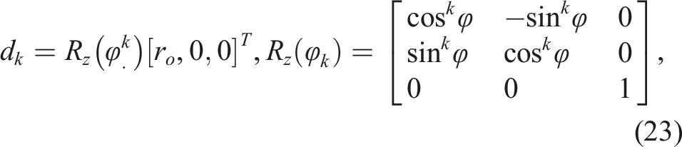
In line with (16), the element compliance distribution 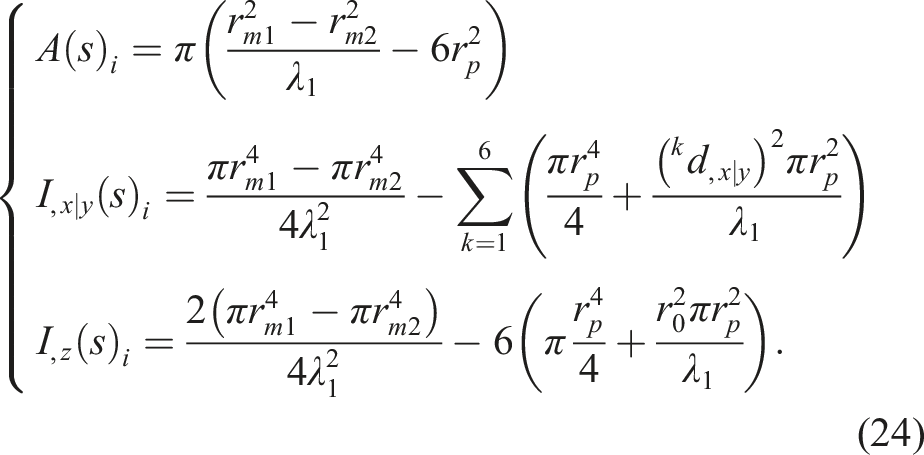
According to Section 2.3, the system parameters from (24) in the (j + 1)th step can be updated via
The actuation variable Ω here is the pressure P in three chamber pairs. According to (12) and (13), the predefined-step method yields
The threshold-based method results in
ΔΩ is replaced by ΔP in following sections.
3.3. Instantiation of the configuration-dependent compliance models
The derivation of the compliance matrix (2) and the corresponding update ((24)) are the same in the PCC and Cosserat rod model. In order to derive the forward kinematics in each step, the actuation wrench needs to be calculated first. In each iteration, the force vector F
P
written in the body frame equals
3.3.1. PCC-based compliance model
As discussed in Section 2.2.1, the set of curvature parameters [κ(s)
i
, s(s)
i
, ϕ(s)
i
] is used to derive the forward kinematics from the ith to the (i + 1)th element. The length of arc s(s)
i
in each iteration is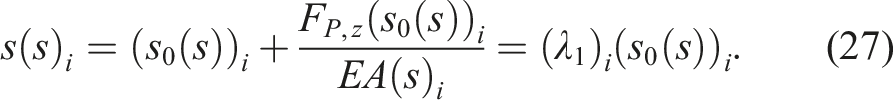
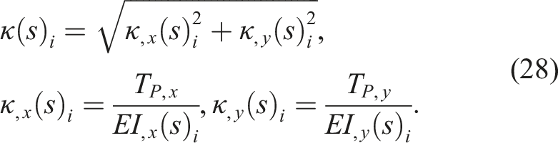
T
P,x
and T
P,y
are the components of moments in the x- and y-axes. The angle ϕ(s)
i
is calculated by
Substituting (27)–(29) to (6)–(5), the PCC-based compliance model in one iteration (i.e., the LPCC model) can be realised.
3.3.1.1. Update principle
Equations (27)–(29) are within one iteration, where the iteration number j is dropped. To update the parameters, the arc parameters in the (j + 1)th step can be treated as the superposition on the jth step according to (15). The initial value of the arc length is updated as 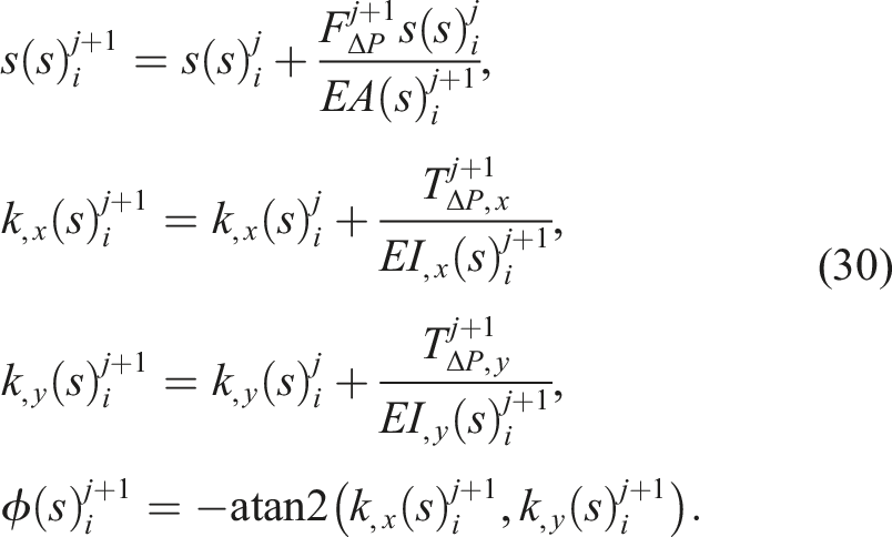
ΔP is the discretised actuation value from (25) or (26). The stretch ratio λ1 in the jth step can be derived and substituted into (24) to update the system parameters. This allows the compliance matrix to be updated in each step.
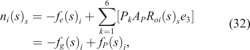
3.3.2. Cosserat rod-based compliance model
Considering the gravitational force f
g
(s)
i
= ρA(s)
i
g, the force equilibrium in a discretised element σ at the position i is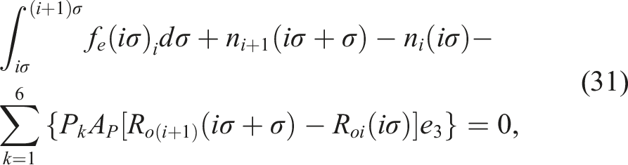
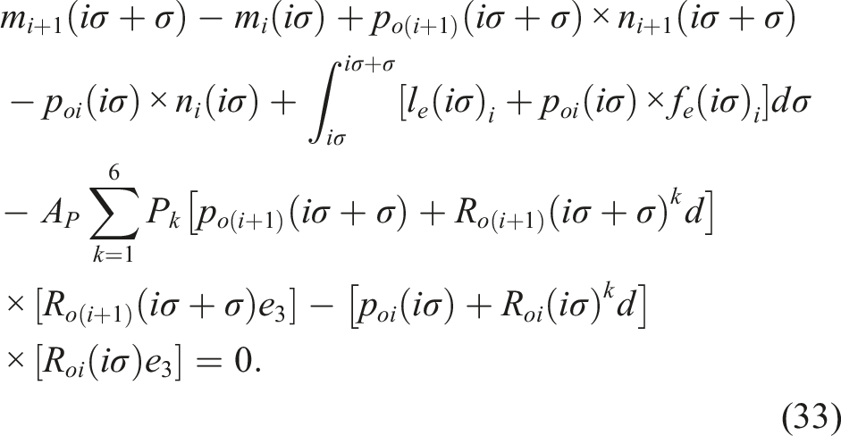
Similar to (32), (33) can be differentiated with σ resulting in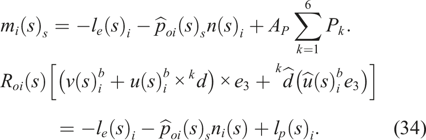
The external distributed moment le(s) i is equal to zero and l P (s) i is the distributed moment resulting from the pressurisation.
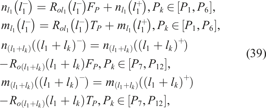
The wrench at the chamber end is balanced by the internal integrated loading [n(l), m(l)], and the exerted external wrench [n
e
(l), m
e
(l)] including the exerted load and the weight of the tip appendage, which includes the sensor and plastic sealing plate, with a total weight of 8 g in this prototype. The boundary conditions can be described by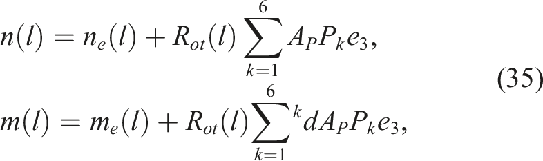
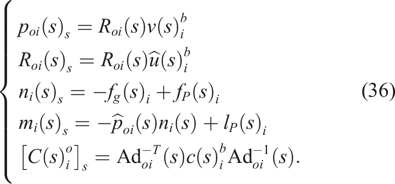
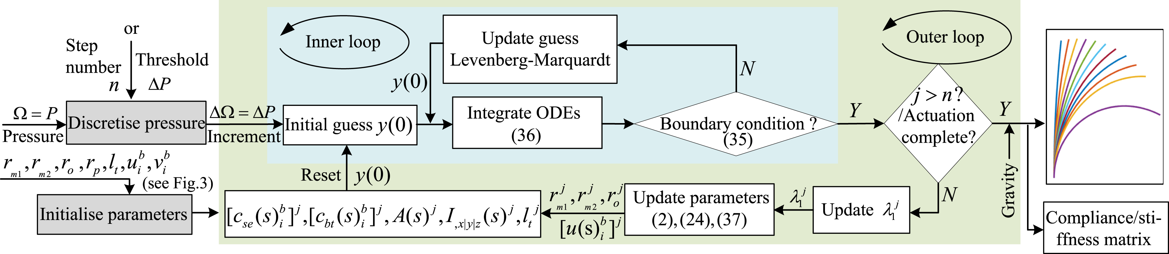
The problem can be solved by (36) with boundary condition (35) (Till et al. 2019). In this paper, (36) is solved using the Fourth-order Runge–Kutta Matlab solver. In this way, the orthonormality of the rotation matrix is maintained during the numerical integration (details are reported in Appendix D). The shooting method is implemented via the embedded optimisation Matlab solver, fsolve (), with the Levenberg–Marquardt method.
3.3.2.1. Update principle
The curvature Implementation scheme of the nonlinear Cosserat method under large elongation. The grey block means it only executes once. The inner loop is to solve the boundary value problem of the set of ODEs in (36). And the outer loop is to deal with the hyper-elasticity resulting from the large elongation and update parameters. The implementation logic is the same for the nonlinear PCC model, by replacing the inner loop (blue rectangle) by the PCC model derived in Section 3.3.1.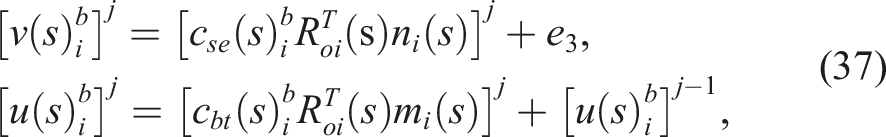
3.3.2.2. Modelling a robot made of two segments
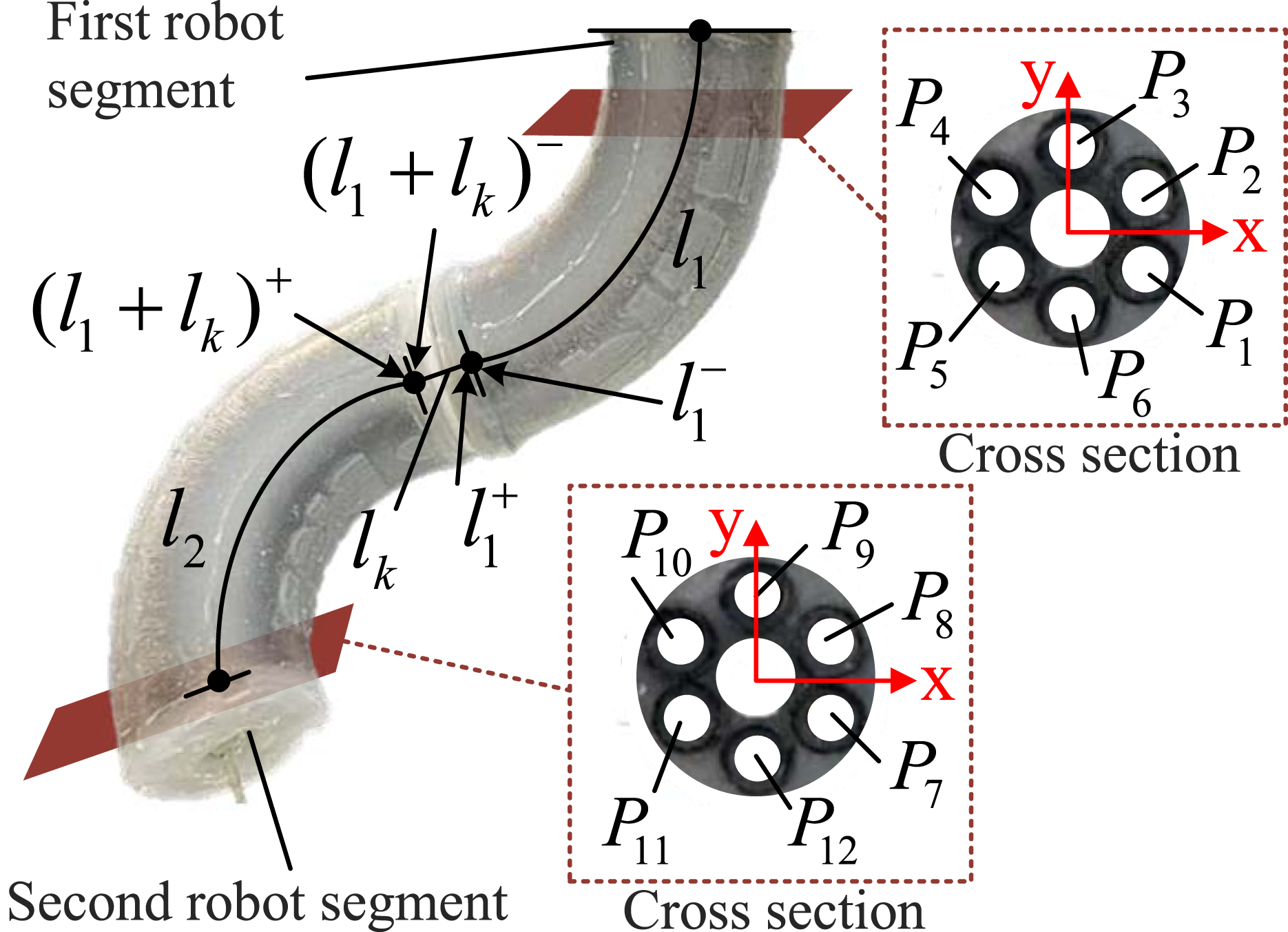
For a soft manipulator made of two robotic segments (see Figure 5), our compliance modelling approach will need to consider intermediate conditions. For the second segment, (31)—(37) can be applied by replacing P1 ∼ P6 with P7 ∼ P12. The connection link is considered as rigid. Firstly, the kinematic continuity between the connection link and two segments (i.e., when s = l1 and s = l1 + l
k
) need to be satisfied which yields (38) Illustration of a robot with two connected segments in series. The dimensions of each segment are listed in Figure 3. The length/thickness of the connection part l
k
is 6 mm. The chamber pressures of the second segment are denoted from P7 to P12.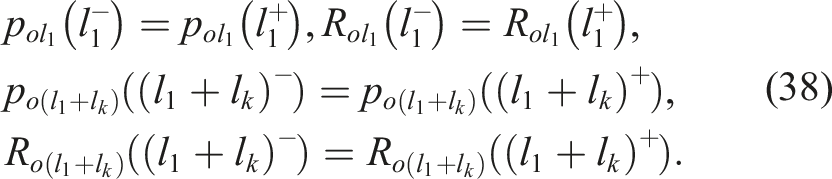
4. Simulation results of the forward kinematics and compliance/stiffness modelling
In this section, computational results are presented based on the established models in Section 3. Simulation 1 presents a comparison of the four forward kinematics models: the linear Cosserat model (LCM), linear PCC model (LPCC), nonlinear Cosserat model (NCM) and nonlinear PCC model (NPCC), and investigates the derived results of the 6 × 6 compliance matrix. The discretised element number in the PCC and Cosserat rod models is chosen as 50 for the interest of compliance integration. Simulation 2 analyses the compliance using the compliance ellipsoid. Simulation 3 presents the configuration-dependent stiffness by the eigenscrew decomposition. In the simulations, the gravity direction is along the −z-axis. In the following sections, we use the terminologies in-plane and out-of-plane bending to denote when the backbone of manipulators bends within a single plane and through different planes, respectively.
4.1. Simulation 1—model implementation and comparison
The first set of simulations compares the LPCC, NPCC, LCM and NCM models. Pressure inputs were in the range of 0–1.5 bar, resulting in the manipulator to bend towards the −x (P1 = P2) or +x (P3 = P4 = P5 = P6) direction. The simulated results when P1 = P2 are illustrated in Figure 6(a), showing that the four models have different kinematic responses. In general, the differences are less for low pressure values (e.g., 0.6 bar). Figure 6(b) reports on the results when two chamber pairs are actuated simultaneously, showing that all four models return similar output when the pressure values are less than 0.3 bar. The NCM and NPCC models have larger bending motions compared to the LCM and LPCC, in particular, when the pressure reaches 1.5 bar. This implies that the consideration of the cross-sectional deformation has a significant influence on the forward kinematics calculations. When comparing the PCC and Cosserat models, it is observed that the Cosserat models result in larger bending angles. Results of Simulation 1 - The bending comparison of the four models when (a) P1 = P2 and (b) P3 = P4 = P5 = P6, with the maximum pressure of 1.5 bar. The soft robotic manipulator bends in the x-z plane.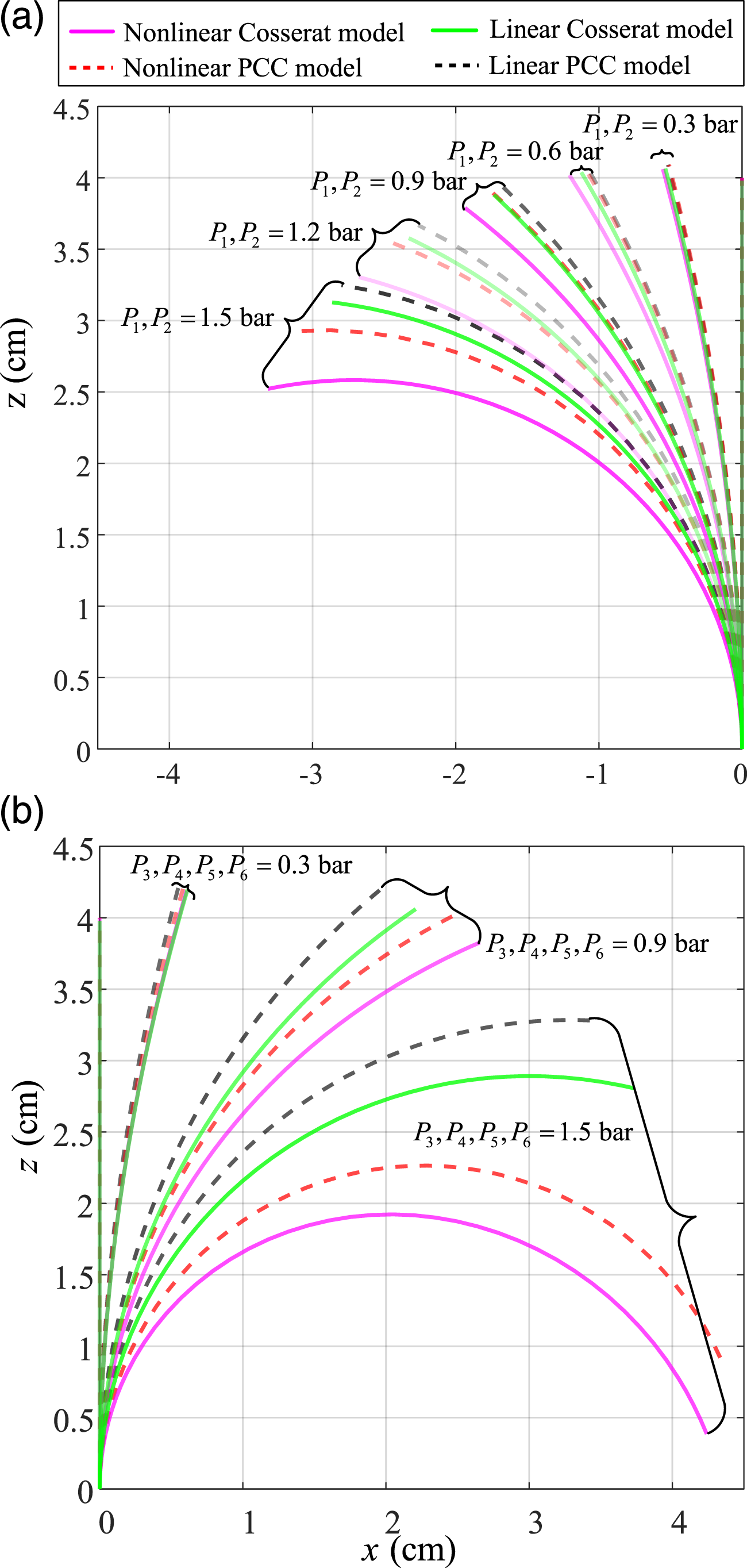
The second set of computational experiments investigates the compliance model when P1 = P2 = 1.5 bar (ϕ = 0°) and P1 = P2 = P3 = P4 = 1.2 bar (ϕ = 240°). The applied external forces Δf
x|y|z
along three main axes ranged between 0.1 ∼ 0.5 N. By integrating the conventional Cosserat rod model (Till et al. 2019) based on the boundary conditions (35), the robot configuration under external forces can be returned. By solving (36) assuming the external force are zero, the configuration-dependent compliance matrix C
o
can be derived first, the configuration subject to external forces can then be obtained from (19) using Co, and the tip wrench 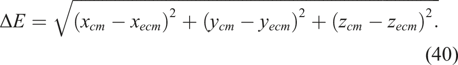
x|y|z
cm
are tip positions from solving the Cosserat model, and x|y|z
ecm
are calculated tip positions yielding from the compliance matrix. Figures 7(a) and (b) show the comparisons of the tip poses under applied forces from direct solving the Cosserat rod model (coloured in black) and from compliance matrix (the red stars). The extracted tip differences ΔE
x|y|z
are shown in Figures 7(c) and (d). It is observed that the differences of the tip position are below 0.15 cm for both in-plane bending cases where ϕ = 0° and ϕ = 240°. Results of Simulation 1, showing the deflections from the 6 × 6 Cartesian compliance matrix, where the star marks is the tip position derived from the compliance matrix, based on (19) and (36). The black lines derive from directly solving the Cosserat rod model, assuming external forces Δfx|y|z are applied at the tip. The results when ϕ = 0° and ϕ = 240° are shown in (a) and (b), respectively. The differences of the tip position ΔE
x
, ΔE
y
, ΔE
z
along the corresponding axes are shown in (c) and (d).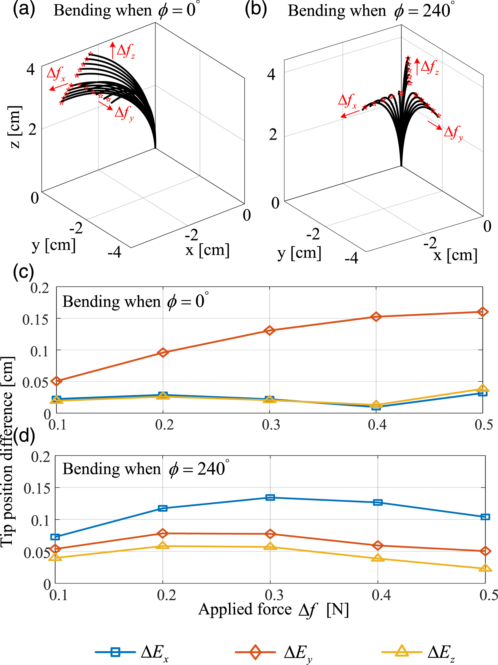
The differences between the nonlinear and linear models become non-negligible especially under high pressure level (see Figure 6(b)). In nonlinear models, high pressure inputs are applied in predefined steps following (25) or (26). Similarly, high external forces can be applied incrementally using the compensation procedures reported in Section 2.3. For Simulation 1, the tip deflection displacements are calculated for small external forces (e.g., below 0.5 N) using two approaches: (1) solving the conventional Cosserat rod model satisfying boundary conditions and (2) calculating the deformed twists from the derived compliance matrix. For in-plane bending with different values of ϕ, both approaches yield similar results. This preliminarily shows the integrated Cartesian compliance matrices are applicable for predicting the deflection displacement under external forces.
4.2. Simulation 2 – Compliance ellipsoid
In line with Section 2.4, the compliance ellipsoid is then adopted to achieve the model-based compliance/stiffness analysis. The nonlinear Cosserat rod model is used in this section. Two sets of simulations were conducted to investigate the compliance distribution along the manipulators under different configurations. The simulation setting is as follows: • Bending and elongation for a robotic manipulator: For the bending simulation, values for P1 and P2 ranged between 0 ∼ 1.5 bar. For the elongation simulation, all chambers were pressurised simultaneously from 0 ∼ 0.9 bar. The difference of pressure values in the two scenarios results in elongation ratios of a similar level. • Bending for a manipulator made of two robotic segments: In the first simulation, P1, P2, P7, and P8 were actuated together. In the second simulation, P1, P2, P9, P10, P11, and P12 were actuated. In both simulations, the pressure was between 0 ∼ 1.2 bar.
Figure 8(a) presents the visualisation of the compliance ellipsoids at 0.5l, 0.6l, 0.7l, 0.8l, l along the manipulator when one chamber pair is actuated. The figure indicates that the compliance monotonically increases from the middle to the tip position, from a lower to a higher pressure. This finding can be quantitatively verified from the extracted minimum and maximum eigenvalues of the compliance matrices. For instance, when the pressure increases from 0 to 1.5 bar, the minimum eigenvalues at the middle and tip position increments from 0.06 to 0.11 and 0.13 to 0.36, respectively. Similarly, the corresponding maximum eigenvalues increases from 0.40 to 0.72 and 1.84 to 3.60. Similar findings can be observed from Figure 8(b), that is, the compliance increases under a higher pressure and at a closer distance to the robot tip. Compared to Figures 8(a) and (b) illustrates the robot becomes more compliant for large bending motions. In particular, the overall maximum and minimum eigenvalues in Figure 8(b) are about 2–3 times higher than the values in Figure 8(a). Figure 8(c) shows the results from the elongation scenario. As occurred in the bending test, it is also observed that the overall compliance increases under high pressurisation. When all the chambers are pressurised to 0.9 bar, the maximum eigenvalue at the tip position reaches 9.34 and increases about five times, compared with the value as 1.84 when the pressure is zero. Results of Simulation 2—the visualisation of the compliance ellipsoids (scaled by a factor of 0.2) with regards to different configurations for a manipulator with one single segment. The corresponding minimum and maximum eigenvalues of the compliance matrices reported at the bottom. Bending when (a) one chamber pair (P1 = P2) is actuated and (b) two chamber pairs (P3 = P4 = P5 = P6) are actuated: the compliance ellipsoid along the manipulator when the pressure increases from 0 to 1.5 bar in 0.3 bar steps. (c) Elongation: the compliance ellipsoids along the manipulator when P1 ∼ P6 increase from 0 to 0.9 bar in 0.3 bar steps.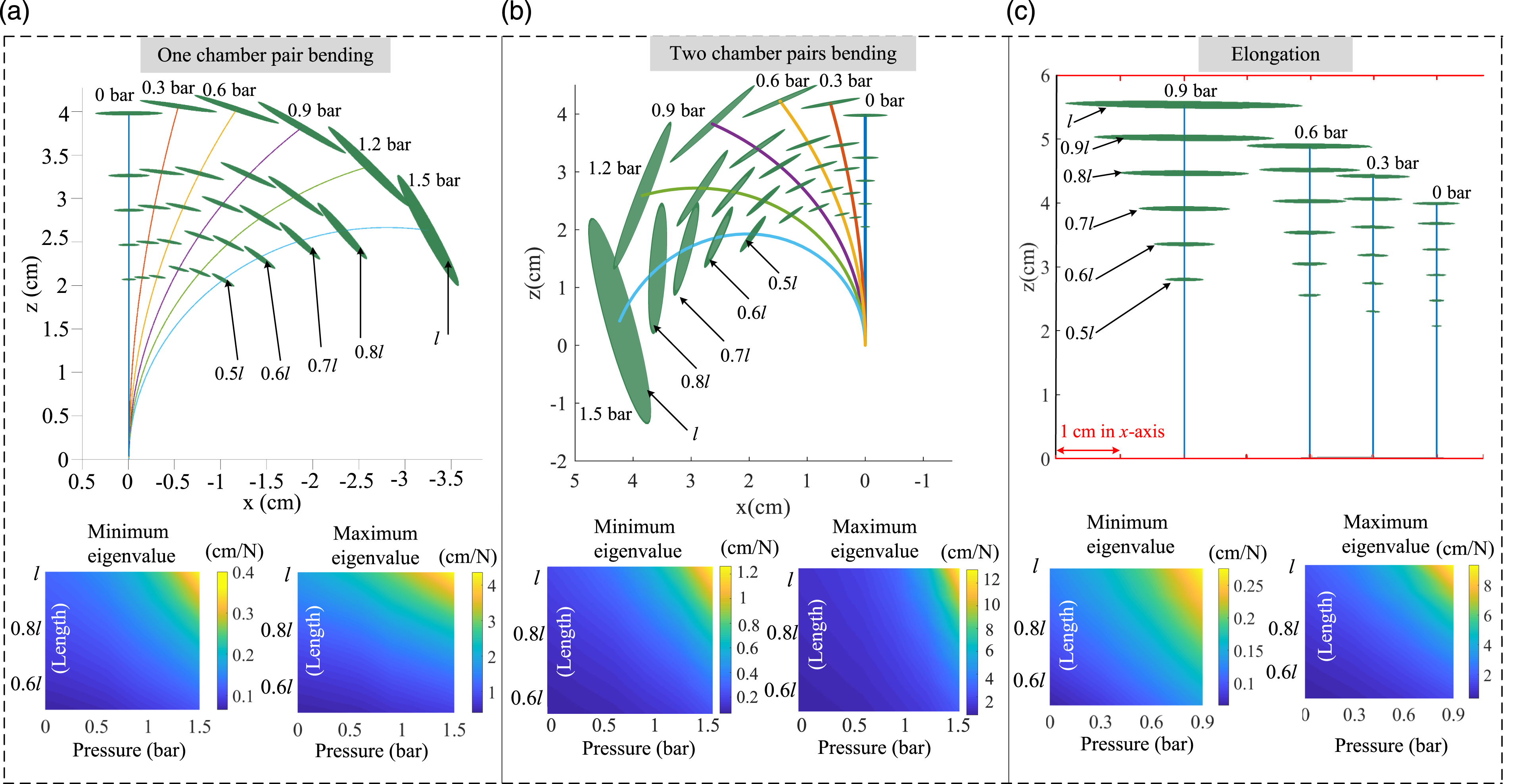
For a manipulator consisting of two robotic segments, the first and second segments are coloured in blue and red, with a 6 mm thick connection part. Figure 9(a) shows the results when P1 = P2 = P7 = P8. It indicates that the maximum and minimum eigenvalues at the tips of both robots increase (e.g., the maximum values increase between 90% ∼ 100%) with increasing pressure, which indicates an overall increase in compliance. The maximum eigenvalues from the tip of the second robot are about 6–8 times larger than the values from the tip of the first robot. The eigenvalues also demonstrate that the compliance of the second robot has a greater variation compared to the compliance of the first robot. Figure 9(b) reports the results when P1 = P2 = P9 = P10 = P11 = P12 with similar conclusions, that is, the tip compliance of the second robot is about 6–8 times larger than the tip compliance from the first robot. Compared to Figure 9(a), the minimum eigenvalues from Figure 9(b) show a smaller variation. Results of Simulation 2 – Compliance ellipsoids (scaled by a factor of 0.1) at the tip of a robot made of two robotic segments, when (a) P1 = P2 = P7 = P8 and (b) P1 = P2 = P9 = P10 = P11 = P12. The pressure increases from 0 to 1.2 bar in 0.3 bar steps. The maximum and minimum eigenvalues of the compliance matrices are reported with the magnitude of the actuation pressure.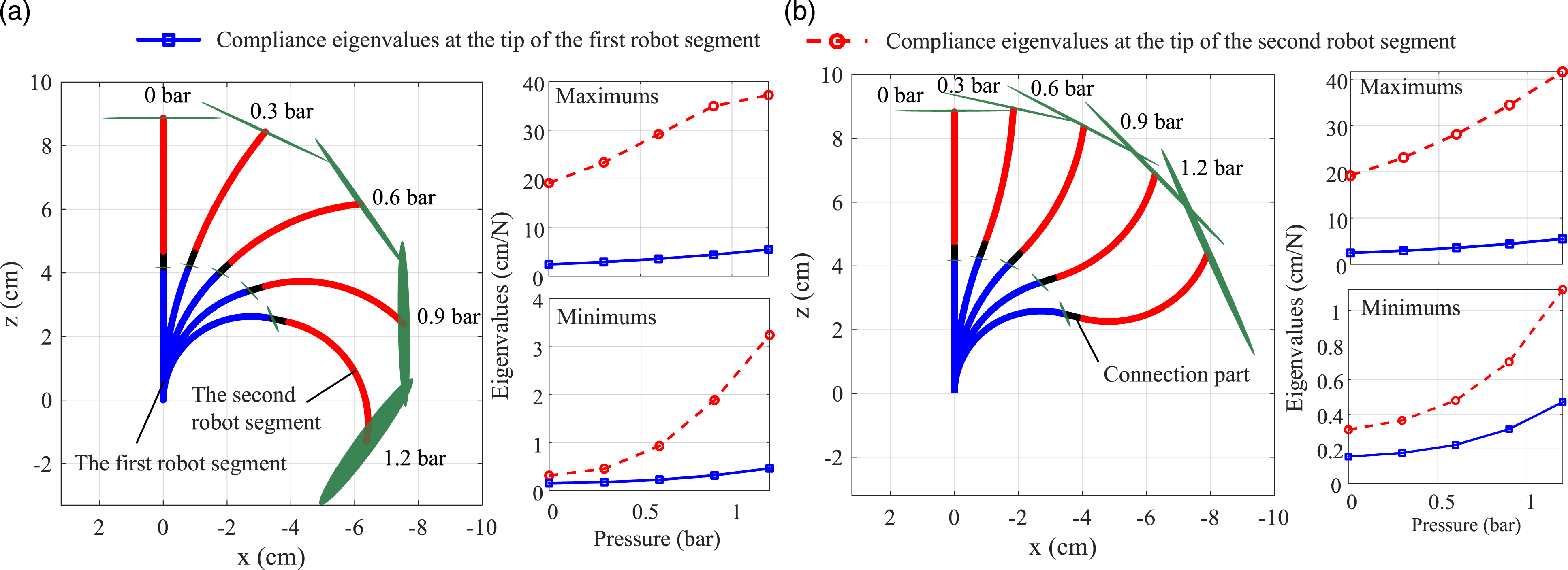
Simulation 2 shows that the distribution of the compliance along the manipulator can be derived based on the forward kinematics models using our proposed method. This is fundamentally different from, for example, the Jacobian projection (Hussain et al., 2021) or using derivatives (Rucker et al., 2011). In particular, (36) describes how the compliance matrices can be integrated with the static Cosserat rod models simultaneously.
4.3. Simulation 3 – Eigenscrew decomposition
To analyse the coordinate-independent stiffness, the eigenscrew decomposition can be derived based on Section 2.4.2. In the simulation, the pressure was in the range of 0–1 bar and implemented using the nonlinear Cosserat Rod model. Figure 10(a) shows the distribution of p
w
, where τ is the maximum positive eigenstiffness. It can be observed the workspace is dome-shaped and enlarged by the elongation. The overall eigenstiffness decreases from 4.37 to 1.49. Results of Simulation 3 – Analysis of stiffness at the tip position based on the eigenscrew decomposition. The maximum and minimum positive eigenstiffness values are extracted and then interpolated using natural method from Matlab to assess the configuration-dependent stiffness, which are displayed from the left to the right side in (b), (c), (d). The maximum pressure in each chamber was 1.0 bar. (a) Demonstration of p
w
. The colorbar illustrates the eigenstiffness attached to the points of workspace. (b) The stiffness projection onto the x-y plane. (c) The stiffness projection onto the y-z plane. (d) The stiffness projection onto the z-x plane.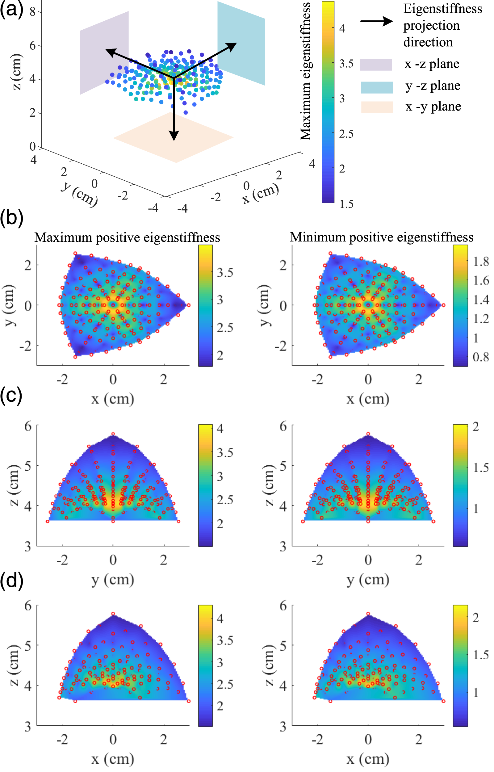
Figures 10(b) to (d) show that both maximum and minimum eigenstiffness values are projected onto the x-y, y-z, and z-x planes. Figure 10(b) shows the stiffness decreases from the centre to the periphery of the workspace. For example, the eigenstiffness value is 4.37 at the centre, but that value is 1.93 at the vertex. Figures 10(c) and (d) convey the same message that the stiffness projected onto the y-z plane and z-x plane also decreases when the workspace becomes larger. Please note that only the enclosed area by the red dotted points shown in Figures 10(b) to (d) is the reachable workspace.
Simulation 3 shows that the stiffness of the manipulator varies in the workspace, and the stiffness capability, described by eigenstiffness (independent from the coordinates), decreases under a high pressure level. Large axial elongation makes the robotic manipulator have more compliant responses. This will be further investigated and validated in Section 5.3.
5 Experimental validation of the forward kinematics and stiffness model
In this section, thorough validation procedures of the proposed method and its results are presented comparing our numerical models (LCM, NCM, LPCC and NPCC) from Section 3.3 with experimental data in Experiments 1–3. Experiments 1–2 use a manipulator made of one segment for validation. Experiment 1 reveals the nonlinear kinematic responses are observed and accommodated. Experiment 2 validates the configuration-dependent stiffness/compliance model. Experiment 3 validates the configuration-dependent compliance modelling using manipulators made of one and two robotic segments.
5.1. Experimental setup
The experimental setup is presented in Figure 11. As shown in Figure 11(a), three proportional pressure regulators (Camozzi K8P) are used to modulate pressurised air in each chamber pair. These are controlled by analogue signals (0 ∼ 10 V) with a pressure feedback channel (0 ∼ 3 bar). A compressor (BAMBI MD Range Model 150/500) is chosen as the pneumatic reservoir supplying constant pressurised air to the pressure regulators. NI-DAQ USB-6341 devices with multiple digital and analogue I/Os are used to monitor and control the pressure regulators. The NI-DAQ USB-6341 provides PWM signals, which are converted to analogue signals (0 ∼ 10 V) by Pulse-Width Modulation (PWM) converters, to control each pressure regulator. In Experiment 3, another three pressure regulators are added and controlled in the same way. Experimental setup. It comprises two subsystems: (a) The hardware for power and actuation mainly contains the air compressor and electronics, such as pressure regulators, PWM converter (denoted using DAC here) and NI USB-6341 boards, to actuate and control the soft robotic manipulator. A laptop running Matlab software collects data and sends control commands. (b) The forward kinematics and stiffness validation setup contains a 7 DoF Franka Emika Panda robot with the soft robotic manipulator mounted on the end-effector, NDI Aurora magnetic trackers, a 6 DoF force/torque sensor, and a linear rail.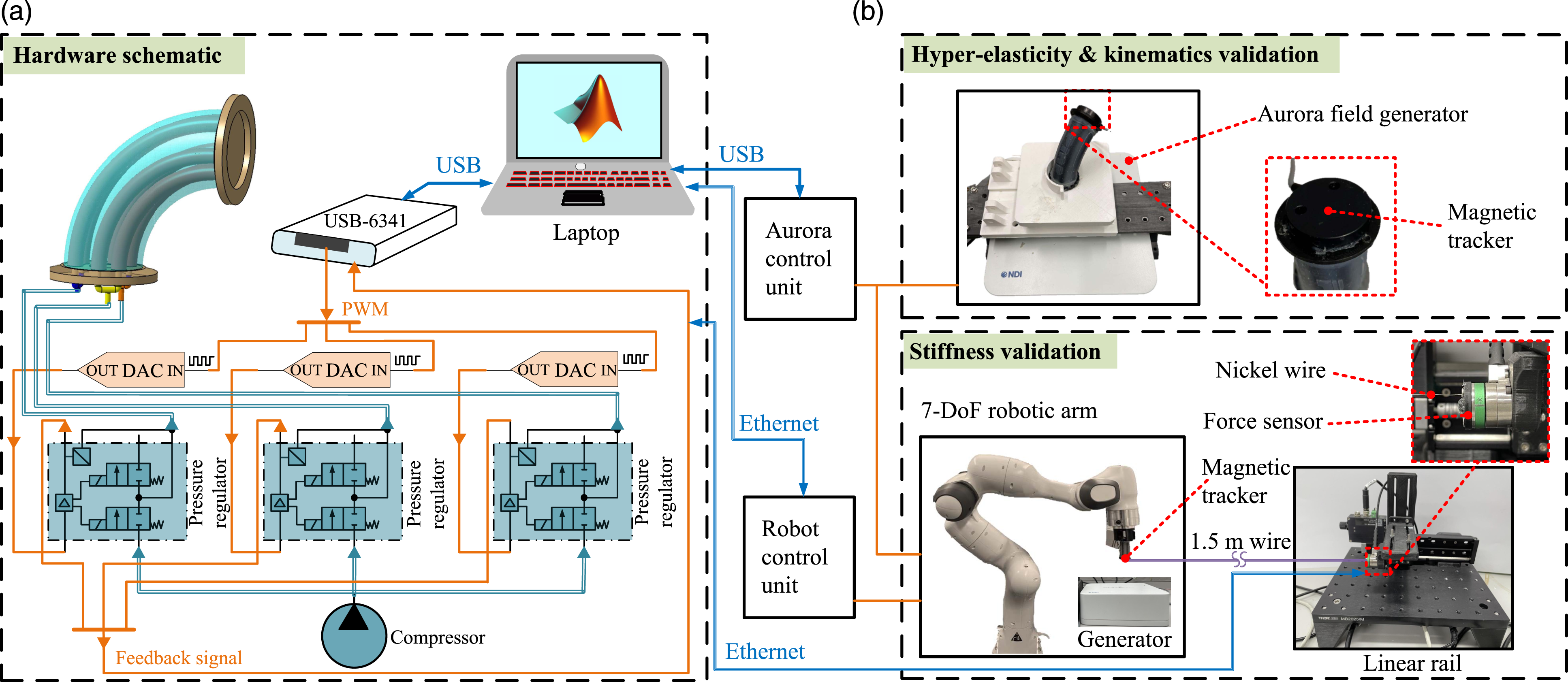
Figure 11(b) shows a 6 Degree-of-Freedom (DoF) Aurora sensor mounted on the tip of the soft robotic manipulator to measure its pose using an NDI Aurora tracking system. The position and orientation tracking errors of the Aurora system (with 6 DoF sensors and a cube volume) are less than 0.48 mm and 0.30°, respectively. Stiffness experiments were conducted by pulling the manipulator’s tip via a 0.19 mm diameter nickel wire connected to an IIT-FT17 6 DoF Force/Torque (F/T) sensor. The F/T sensor was mounted on a motorised linear rail (Zaber X-LSM100 A), which controlled the pulling speed and displacement. A 1.5 m length wire was chosen to guarantee a high confidence in the angle of the applied pulling force. For instance, when Δf x is applied along the x-axis, a 1 cm displacement error in the z-axis would result in an angular error of about arctan 0.01/1.5 = 0.38°, which is negligible. For the stiffness validation experiments, the soft manipulator was fixed to a 7 DoF robotic arm (Franka Emika Panda) to arrange the desired pose and measure the configuration-dependent stiffness. All hardware was connected to a laptop running Matlab software to capture data, control the soft robot and the 7 DoF robotic arm, and post-process the acquired data.
5.2. Experiment 1 – Validation of the forward kinematics and nonlinear compensation
To validate the forward kinematics and the nonlinearity, three sets of experiments were conducted by pressurising one, two and three chamber pair(s) simultaneously. When one chamber pair was pressurised, the pressure was from 0 to 1.5 bar and followed the sequence: (P3, P4 → P5, P6 → P1, P2). When two chamber pairs were pressurised, the pressure was from 0 to 1.2 bar and followed (P1, P2, P3, P4 → P3, P4, P5, P6 → P1, P2, P5, P6). When three chamber pairs were actuated, the pressure in all six chambers was from 0 ∼ 1.2 bar and increased simultaneously. During these experiments, the tip position of the soft manipulator and chamber pressures were recorded at 40 Hz. The maximum pressure values in both bending experiments were set differently, so the maximum bending angle reached the same value in both experiments. The pressure was incrementally increased by 0.15 bar. In the simulation, the threshold-based method was chosen to discretise the pressure with a threshold value of 0.15 bar, when one chamber pair was pressurised according to (26). The finite-step method was chosen with n = 6, when two chamber pairs were pressurised based on (25).
Figure 12 illustrates extracted static elongation and bending angles. The experimental data are plotted in blue circles and linearly interpolated by curve fitting (see blue curve). The LCM, NCM, LPCC and NPCC are plotted in green, magenta, dotted black, and dotted red, respectively. In addition, the elongation ratio is displayed at the bottom of Figures 12(a) to (c), derived by computing the change of the length of the backbone of the manipulator over the default length. Proportionality constants are 0.4 cm, 52.5°, and 30.0° per 0.1 of the elongation ratio in Figures (a), (b) and (c), respectively. Figures 12(b) and (c) report the elongation ratios for the purpose of illustrating the level of elongation when the robot has a bending motion. From Figure 12(a), it can be seen that the manipulator achieves a maximum elongation of 2.7 cm. The results of all numerical models and experiments are similar for pressures up to 0.45 bar and an elongation ratio of 0.15. Above these values, the curves of the LCM and LPCC behave in a linear way compared to the two nonlinear models and experiments. The overall Root Mean Square Error (RMSE) of two nonlinear models is 0.07 cm, while the RMSE of two linear models is 0.49 cm (see Table 3). Results of Experiment 1 – nonlinear kinematic responses: Experiments are compared to results from (non)linear models. Applied pressures are plotted against (a) elongation displacement and elongation ratios when all chamber pairs are actuated, and angles and elongation ratios when (b) one chamber pair and (c) two chamber pairs are pressurised. The orange stars demonstrate the level of elongation when any nonlinearity becomes significant. (a) Reports the elongation ratios from experiments; (b) and (c) report the ratios from the NCM. Comparisons are reported on in Extension 1. Summary of results for Experiment 1: Comparison of errors for the linear and nonlinear simulation models with experiments.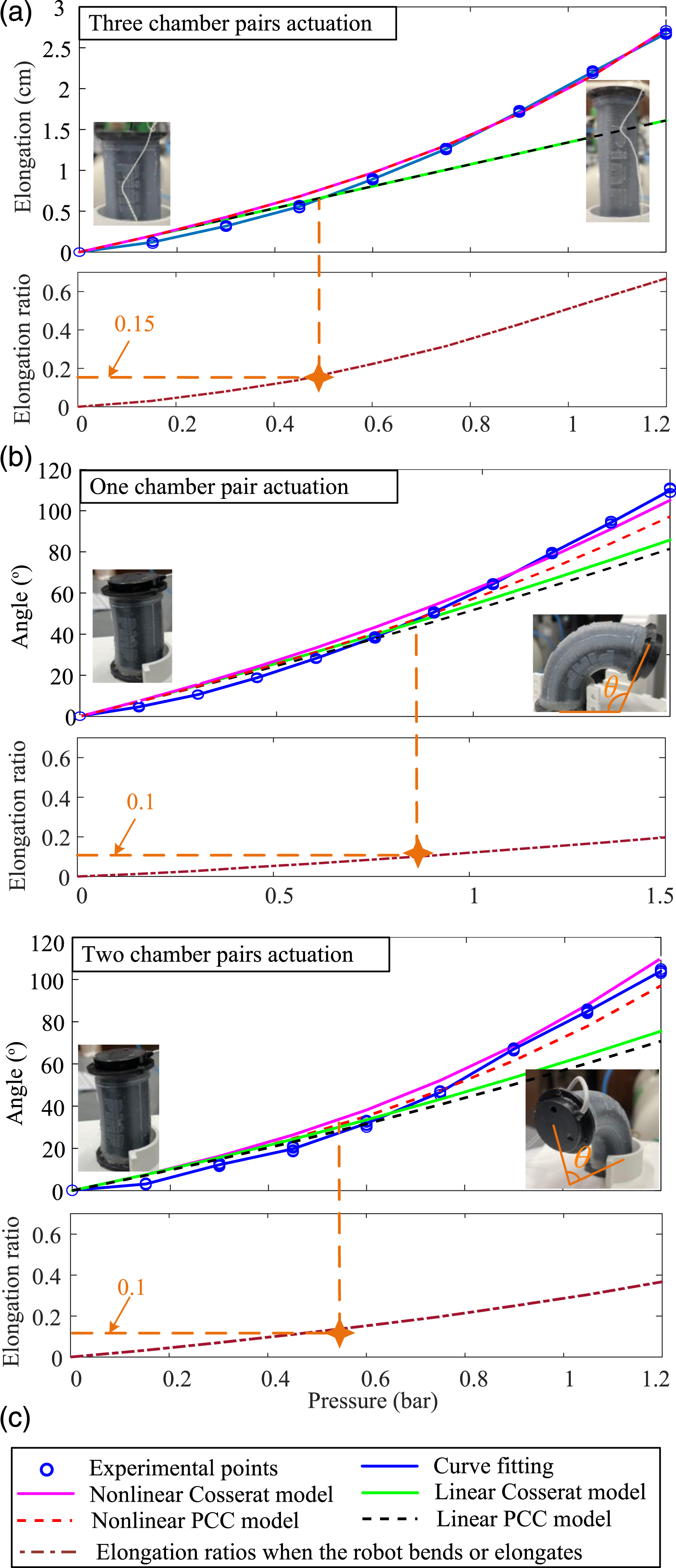
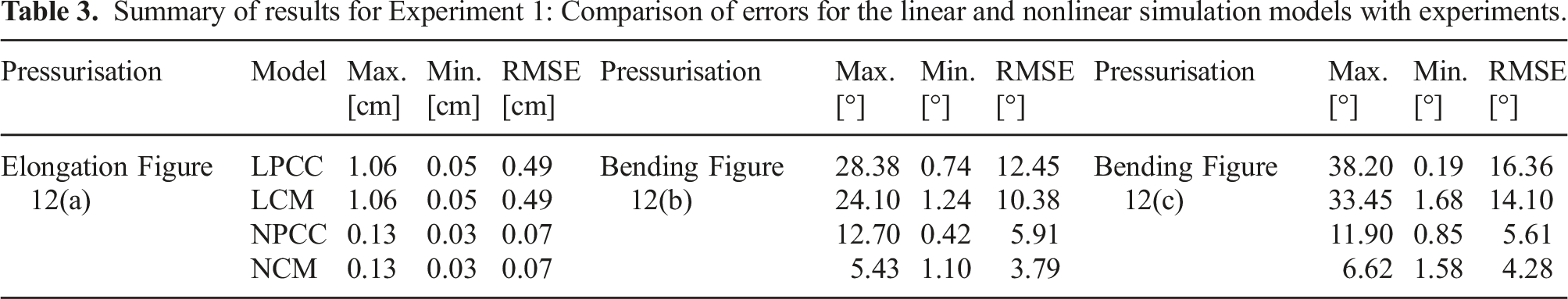
In Figures 12(b) and (c), the maximum bending angles are similar and around 110°. The maximum elongation ratio is about 0.2 and 0.4 when one and two chamber pairs are pressurised. The nonlinearity is notable when the elongation ratio is larger than 0.1. The nonlinear models outperform linear model sets. For example, the NCM shows the smallest RMSE in two bending scenarios, which are 3.79° and 4.28°. By comparison, the linear models are less accurate. Specifically, the LCM, with the RMSE of 10.38° and 14.10°. Moreover, the Cosserat rod models show a better performance that the PCC models. A detailed summary of the errors is shown in Table 3.
Figure 13 shows the results for the forward kinematics validation, with detailed summary of errors in Table 4. The top row plots of Figure 13 show the triangular-shaped pressurisation pattern of the chamber pairs followed by corresponding position measurements. The bottom two rows plot the positional error for the (non)linear Cosserat rod and PCC models compared to the experimental results in the x-, y-, and z-directions. Results of Experiment 1 – Forward kinematics validation: (a) One chamber pair actuation with pressure amplitudes of 0.9, 1.2, and 1.5 bar. (b) Two chamber pairs actuation with pressure amplitudes of 0.6, 0.9, and 1.2 bar. x
exp
, y
exp
, and z
exp
are the experiment positions. x
sim
, y
sim
, and z
sim
are the simulation results for the nonlinear Cosserat model. Summary of results for Experiment 2: Tip position errors.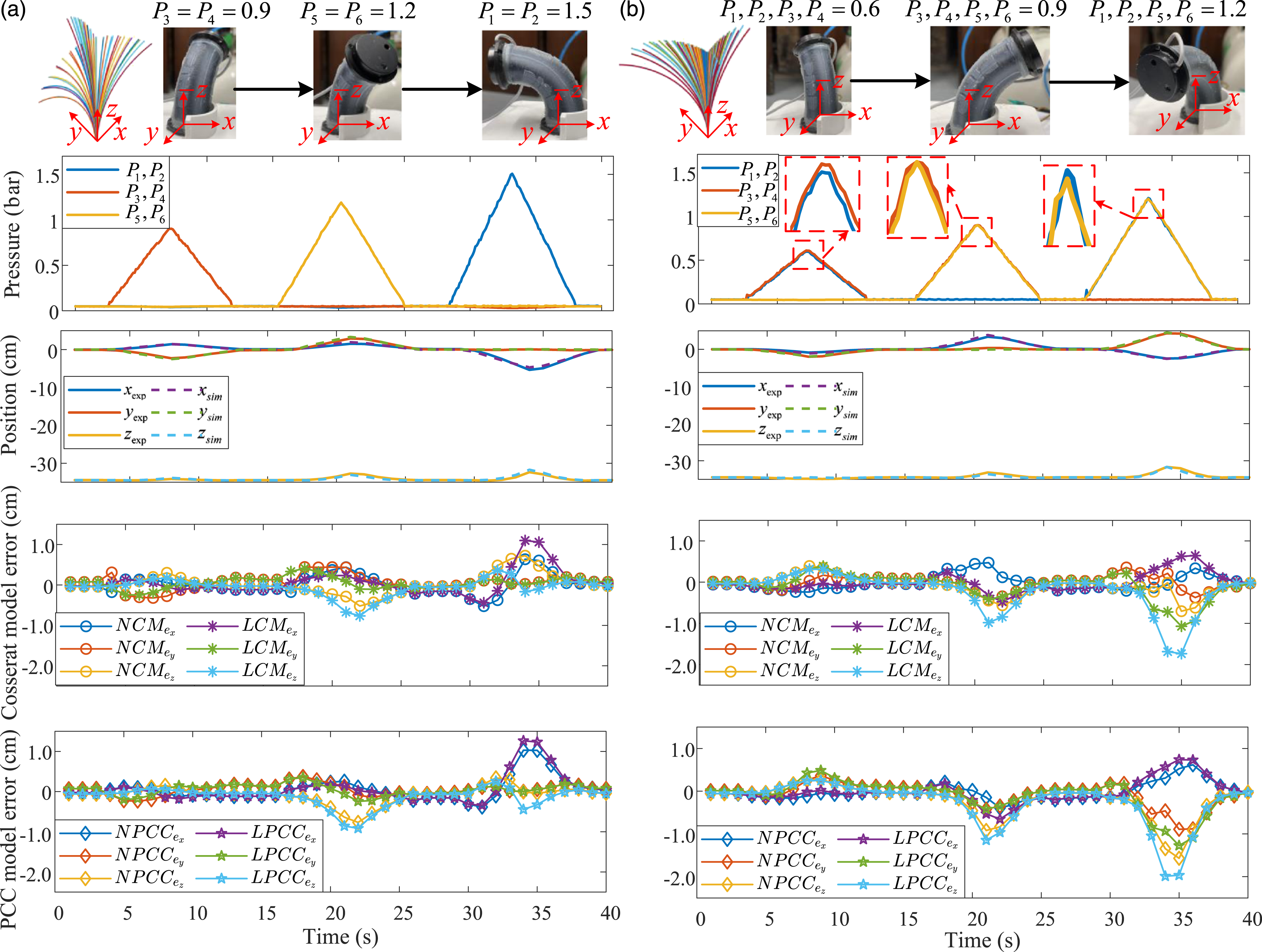
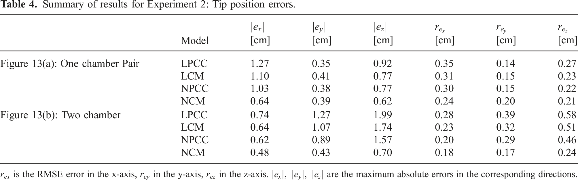
Figure 13(a) shows the forward kinematics results when one chamber pair is pressurised with different amplitudes. During 2.5 ∼ 12 s, the errors of the linear and nonlinear models are similar for this value of pressurisation. During 15.5 ∼ 25 s, the amplitude is set to 1.2 bar, resulting in an increase of the error values for two linear models. The maximum error reaches 0.76 cm for the LCM and 0.91 cm for the LPCC. This error further increases during 28.5 ∼ 38 s, when the maximum pressure is 1.5 bar. In this instance, the maximum error in the x-axis is 1.03 cm for the NPCC and 0.64 cm for the NCM. This error is larger for the linear models (1.26 cm for the LPCC and 1.09 cm for the LCM).
Figure 13(b) shows the results when two chamber pairs are pressurised. Similar to Figure 13(a), the error values of the four linear and nonlinear models are almost identical and below 0.5 cm, when the pressure inside each of the two chamber pairs is below 0.6 bar during 2.5 ∼ 12 s. The discrepancy between the linear and nonlinear models again becomes larger with the increase of the pressure. For instance, when the pressure is increased to 1.2 bar, the maximum errors in the x-, y-, and z-directions for the LCM are 0.64, 1.07, 1.74 cm. Conversely, the errors of the NCM are 0.47, 0.43, 0.70 cm in three directions. Overall, the NCM returns the highest accuracy with an RMSE value below 0.24 cm compared to RMSE values of 0.46, 0.51, 0.58 cm for the LCM, NPCC, and LPCC (see Table 4).
5.3. Experiment 2 – Validation of the stiffness and compliance for a one robotic segment
Two types of experiments are used to validate the compliance/stiffness modelling. The translational compliance matrix 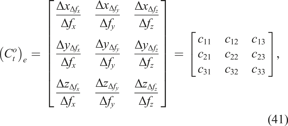
For planar stiffness validation (Shiva et al., 2016; Ranzani et al., 2016), the manipulator had planar motions, within the x-z plane. The stiffness along the x-, y- and z-axes was investigated. When the manipulator bent to the -x-axis, the pressure of P1 and P2 was in the range of 0 ∼ 1.5 bar. When the manipulator bent to the +x-axis, the pressure of P3, P4, P5, and P6 was in the range of 0 ∼ 1.2 bar. For Cartesian compliance validation, the 3 × 3 compliance matrix
Figure 14(a) shows the stiffness response in three directions (i.e., x-, y-, and z-axes) with one chamber pair pressurised. As the bending angle increases due to pressurisation up to about 0.9 bar, the experimentally acquired stiffness values along the x-axis decreases first and then reaches a bending angle of about 90° with a maximum stiffness of 1.21 ± 0.17 N/cm. The four models return different error values when compared with the experimental results. The errors between all models and the experimental data are within 0.10 N/cm when the pressure is less than 0.6 bar. When the pressure further increases to 1.5 bar, the error is 0.28 ± 0.17 N/cm for the NCM, 0.05 ± 0.17 N/cm for the LCM, 0.47 ± 0.17 N/cm for the NPCC, and 0.42 ± 0.17 N/cm for the LPCC. By contrast, the overall stiffness monotonically decreases in the y-direction, from 0.57 ± 0.04 N/cm to 0.27 ± 0.02 N/cm. The error values of the two nonlinear models are within 0.05 N/cm. The error is larger than 0.10 N/cm for the linear models. The overall stiffness also decreases in the z-axis, from 7.33 ± 0.33 N/cm to 0.42 ± 0.03 N/cm. Results of Experiment 2 – Planar stiffness along the x-, y-, and z-axes. (a) Stiffness response when P1 and P2 are actuated and between 0 ∼ 1.5 bar. (b) Stiffness response when P3, P4, P5, and P6 are actuated and between 0 ∼ 1.2 bar. The experimental data points are plotted using blue circles. Stiffness is calculated from the measured displacement and force data. The shaded areas in orange colour span from the minimum to maximum stiffness values. The computational results from our models are plotted in a solid pink, green as well as dotted red and black coloured curve.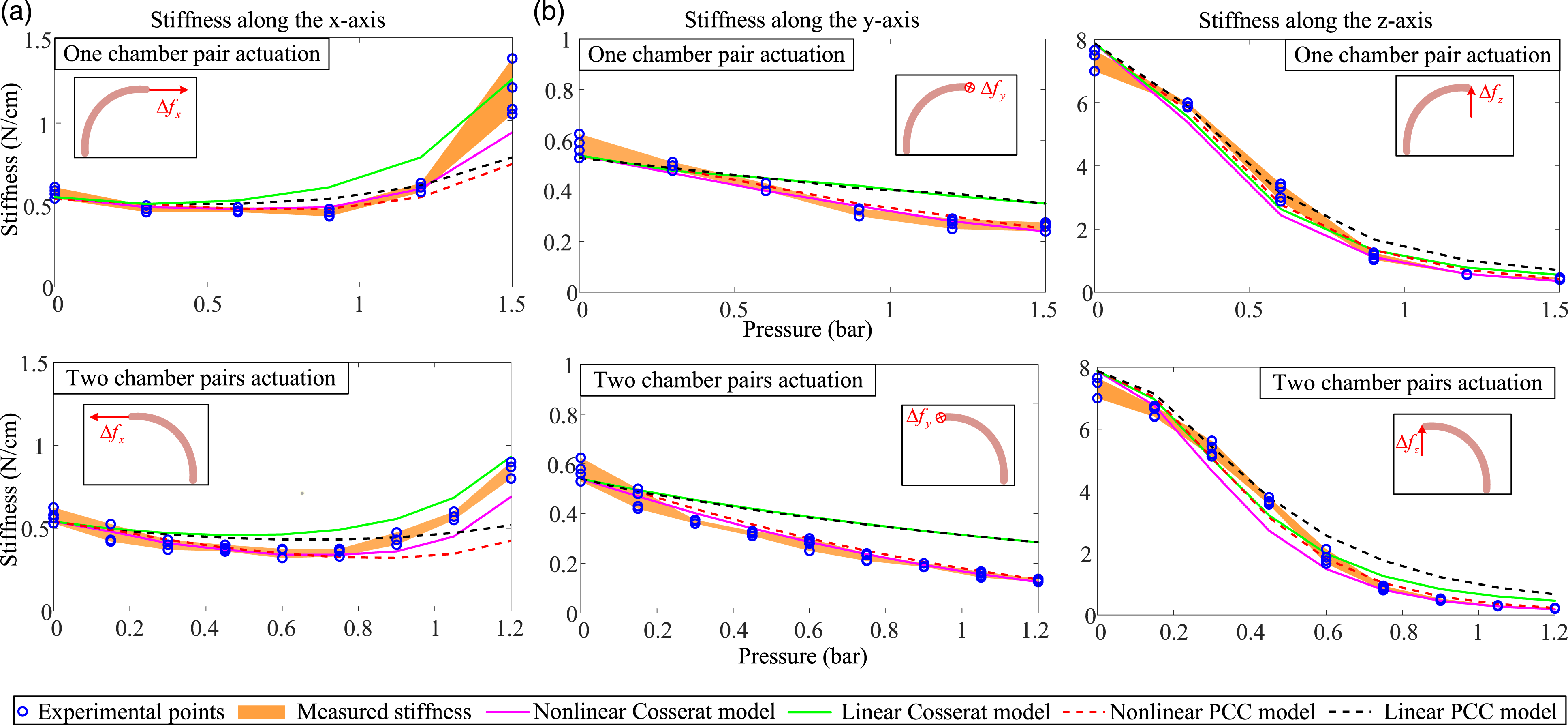
Figure 14(b) shows the results when two chamber pairs are pressurised. The stiffness response in all directions follows a similar pattern. However, all stiffness values are lower. For example, the stiffness value in the y-direction is 0.27 ± 0.02 N/cm in Figure 14(a); this value is about two times lower (0.12 ± 0.01 N/cm) in Figure 14(b). As mentioned earlier, the pressurisation of one chamber pair with 1.5 bar and two chamber pairs with 1.2 bar each achieve a bending angle of approximately 90°. In line with previous results, the modelling errors of the linear models increase with the pressure. For instance, at a bending angle of about 90°, the maximum stiffness error along the y-axis is 0.08 ± 0.02 N/cm when one chamber pair was pressurised and 0.16 ± 0.01 N/cm when two chamber pairs are actuated.
To quantitatively assess the accuracy, the Frobenius norm is utilised, and the error e
C
in (42) is defined as the difference of the Frobenius norm between the simulated and experimental compliance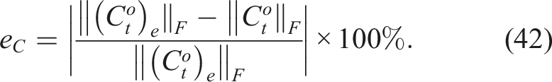
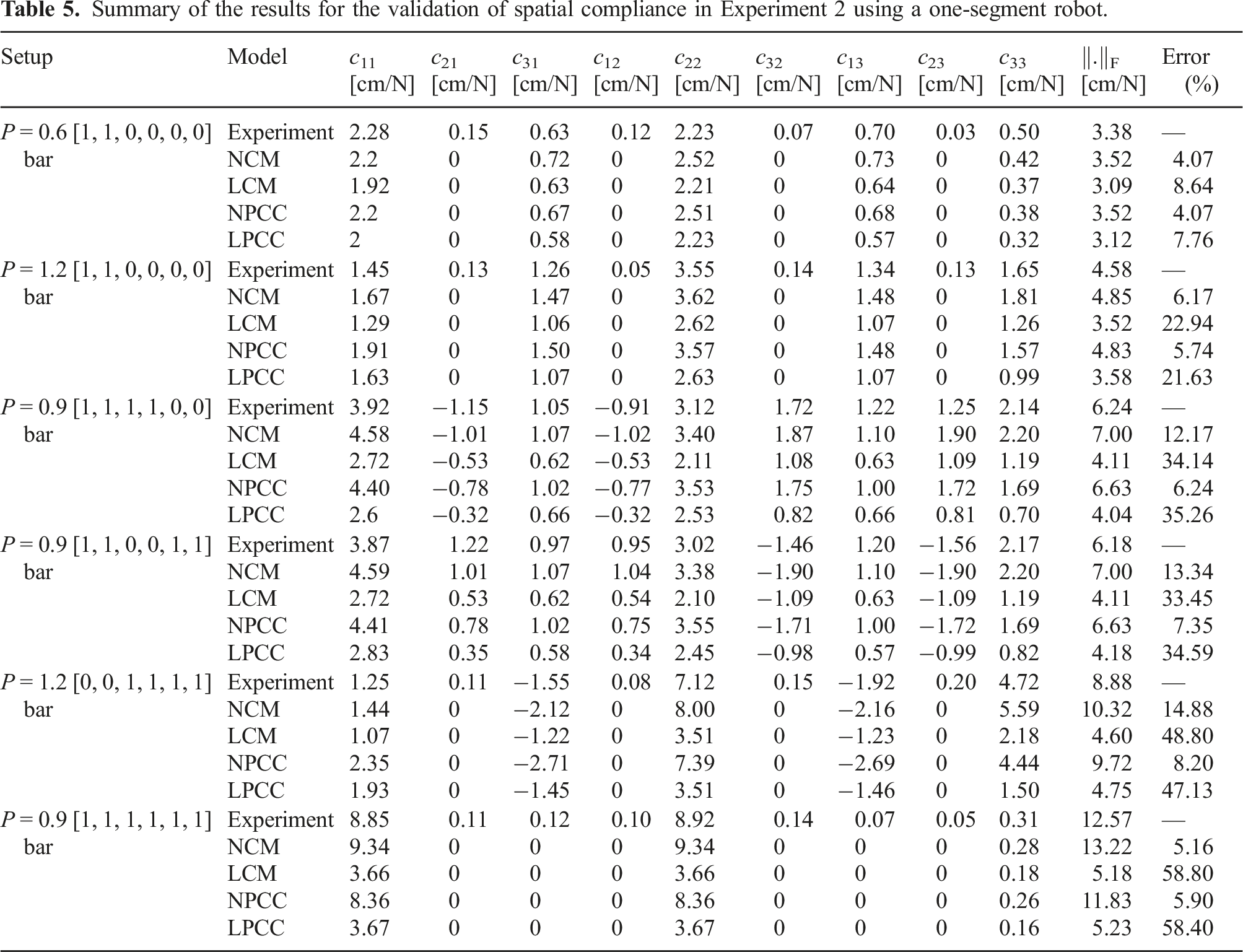
Summary of the results for the validation of spatial compliance in Experiment 2 using a one-segment robot.
Furthermore, the compliance ellipsoids when P = [0.9, 0.9, 0.9, 0.9, 0, 0] bar are projected in Figure 15. Each row, from left to right, shows the ellipsoids’ projection onto the x-y, y-z, and x-z planes for Δf = [0.5 cos θ, 0.5 sin θ, 0] N, Δf = [0, 0.5 cos θ, 0.5 sin θ] N, and Δf = [0.5 cos θ, 0, 0.5 sin θ] N in Figures 15(a) to (c), respectively. The results demonstrate that both linear models and both nonlinear models return a similar performance. The size of the major and minor axes of the compliance ellipsoids from the two linear models return large errors. Results of Experiment 2 – Ellipsoid visualisation of the compliance matrices. NCM, LCM, NPCC, LPCC represent the simulated compliance from the nonlinear Cosserat, linear Cosserat, nonlinear PCC and linear PCC model, separately. The compliance ellipsoid is shown for P = [0.9, 0.9, 0.9, 0.9, 0, 0] bar and projected onto the x-y, y-z, and x-z plane from the left to the right column for (a) Δf = [0.5 cos θ, 0.5 sin θ, 0] N, (b) Δf = [0, 0.5 cos θ, 0.5 sin θ] N and (c) Δf = [0.5 cos θ, 0, 0.5 sin θ] N, with θ = 0 ∼ 2π.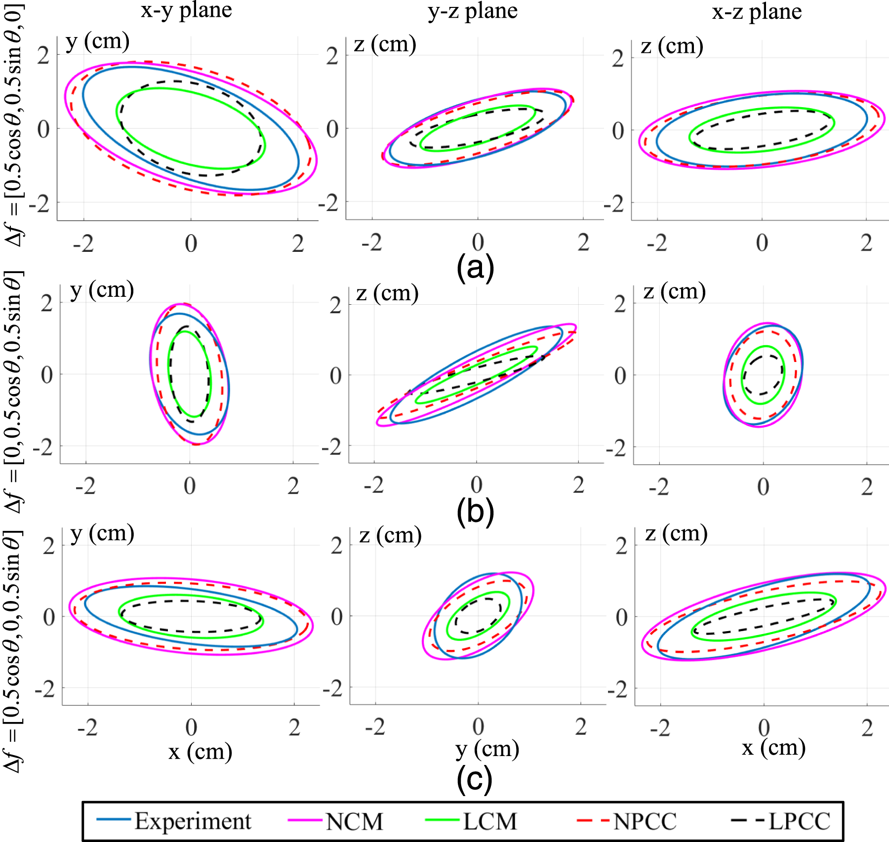
5.4. Experiment 3 – Validation of the compliance for a robot made of two robotic segments
The results of Experiment 3 validate our approach for a manipulator made of two robotic segments, where the robot can generate out-of-plane bending. As reported in Experiments 1–2, the NCM method provides the most accurate forward kinematics and compliance modelling. Therefore, we selected the NCM method for validation in this section. During the experiments, the two robotic segments were actuated achieving six configurations with actuation pressures ranging from 0.6 to 1.2 bar. Similar to Experiment 2, the overall tip compliance was experimentally determined using (41). The pulling forces Δf were applied using calibrated 1 g and 2 g weights, and the corresponding displacements were recorded by an Aurora tracker attached to the overall tip. Compliance errors between simulations and experiments were described using Frobenius norms and defined by (42). Extension 3 reports on the compliance measurement in this experiment.
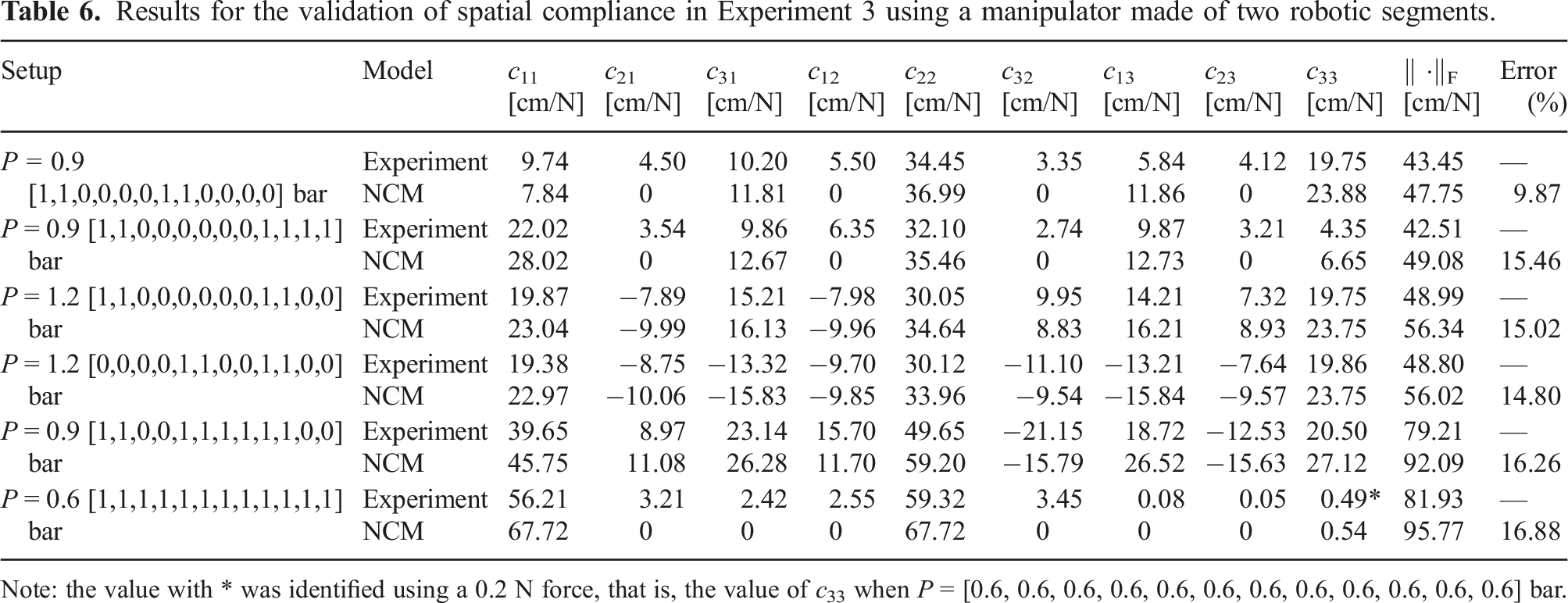
Figure 16 displays the simulated compliance ellipsoids for a manipulator made of two segments and the captured robot images from experiments under six configurations. The compliance ellipsoids are scaled by a factor of 0.1 for visualisation purposes. The two robots are coloured in blue and red, and the connection part is black. The figure demonstrates that our model is applicable to robots made of two robotic segments and is highly aligned with the experimental results, returning maximum tip position errors of less than 6.0 mm. Table 6 details the validation results for the compliance matrices. The results show that the compliance modelling errors, evaluated by Frobenius norms, are between 10% ∼ 20%. Compared to the Frobenius norms of the compliance matrices from Table 5, the values in Table 6 at the tip of the robot made of two robotic segments are generally 5 ∼ 10 times larger. For instance, forces on the order of 0.1 N typically result in displacements on the order of 1 cm when the robot made of two robotic segments has a bending motion. In contrast, tip forces on the order of 1 N produce displacements on the order of 1 cm for one robotic segment. The tip compliance of the robot made of two robotic segments exhibits significant compliant behaviour in the x- and y-directions, while the compliance along the z-axis is much smaller, as shown in Figure 16(f) and the last row of Table 6. Results of Experiment 3 – Simulated compliance ellipsoids at the tip of a manipulator of two robotic segments under six configurations when (a) P1 = P2 = P7 = P8 = 0.9 bar, (b) P1 = P2 = P9 = P10 = P11 = P12 = 0.9 bar, (c) P1 = P2 = P9 = P10 = 1.2 bar, (d) P5 = P6 = P9 = P10 = 1.2 bar, (e) P1 = P2 = P5 = P6 = P7 = P8 = P9 = P10 = 0.9 bar, and (f) P1 ∼ P12 = 0.6 bar. An image of the robot’s configuration from experiments is included with the simulations. The experimental and simulated overall tip positions are presented with the unit of cm. Results for the validation of spatial compliance in Experiment 3 using a manipulator made of two robotic segments. Note: the value with * was identified using a 0.2 N force, that is, the value of c33 when P = [0.6, 0.6, 0.6, 0.6, 0.6, 0.6, 0.6, 0.6, 0.6, 0.6, 0.6, 0.6] bar.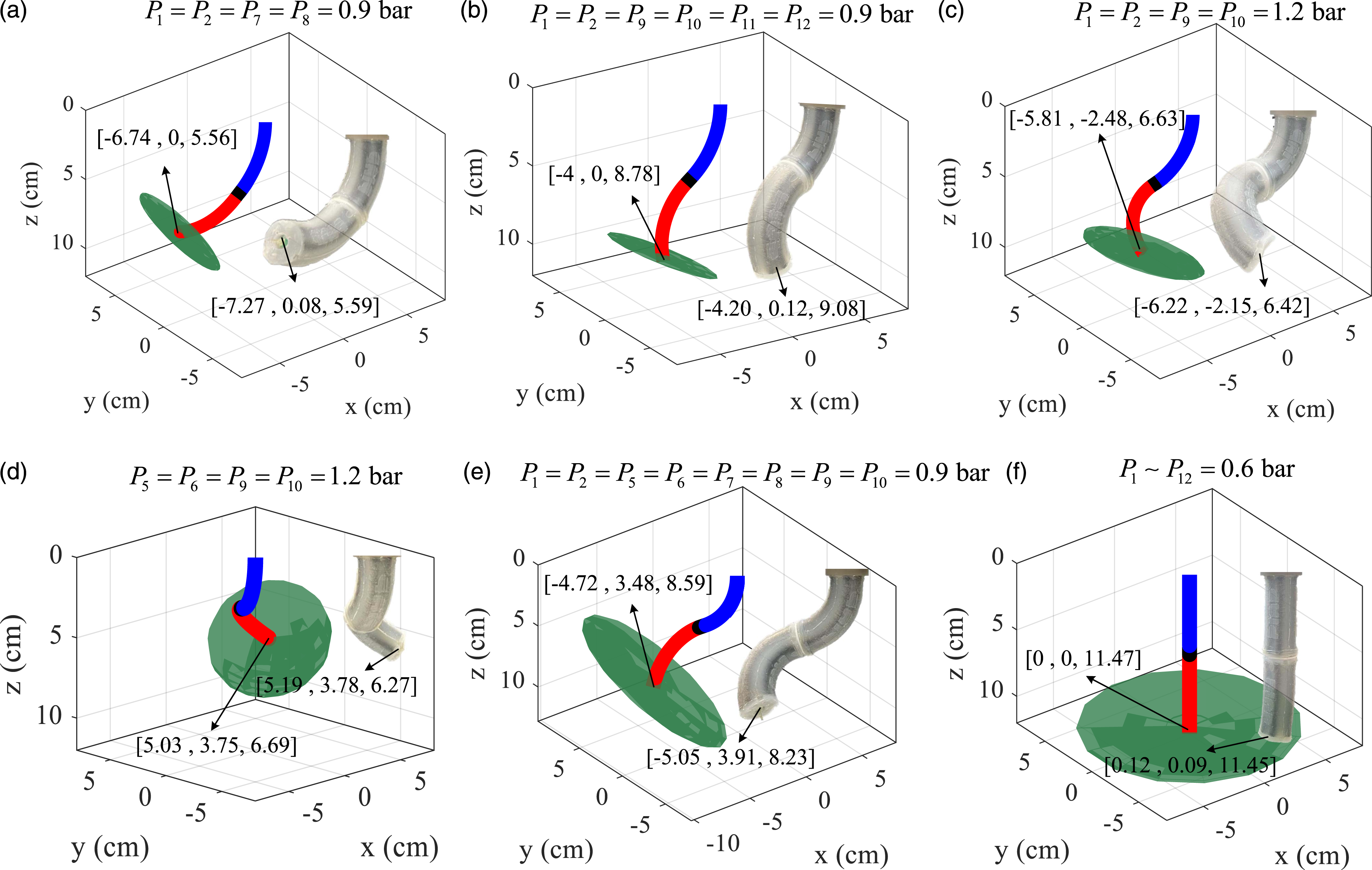
6. Discussions and conclusion
To model the stiffness/compliance of soft robots and achieve the configuration-dependent stiffness analysis, a Lie theory–based stiffness modelling and analysis framework was proposed and experimentally validated using soft manipulators made of one and two robotic segments. In addition, a thorough stiffness/compliance analysis is presented both from simulation and experiment. The main findings of soft manipulators with an elongation capability can be summarised as 1. Large elongations in soft robotic manipulators often introduce nonlinear responses. We proposed two model sets, linear model sets (LPCC and LCM) for small elongations and nonlinear model sets (NPCC and NCM) for large elongations. This improves the modelling accuracy in both forward kinematics and stiffness/compliance. 2. The overall compliance of soft manipulators is influenced by the elongation, for example, the used pneumatic-driven manipulators show compliant behaviours under a high pressure level.
6.1. Nonlinear compensation
Experiment 1 shows the nonlinearity appears for an elongation ratio over 0.15 in cases of elongation (see Figure 12(a)) and 0.1 in cases of bending (see Figures 12(b) to (c)). Below these elongation ratios, the material deforms in a linear manner. The results show that these nonlinearity can be captured by the proposed compensation method, for the nonlinear Cosserat rod and PCC model both show a satisfactory efficacy reproducing the nonlinear responses compared to the linear models. The nonlinearity introduced by elongation further influences the forward kinematics of robots, with the increase of the pressure (see Figure 13). In addition, the results show that both Cosserat models return lower error values compared to the PCC models, as the constant curvature might not be strictly satisfied. Further, the predicted elongation displacement and bending angle of the four models in Figure 12 are slightly higher than the measured results when the pressure is low, which may come from the linearisation of the material model.
Our framework’s nonlinear compensation procedures are based on the theoretical support of the nonlinear matrix structure analysis approach outlined in Gazzola et al. (2018). This allows our framework to consider large deformations using a linear strain–stress relation without the need to change the fundamental models. Similar updates have been reported in (Gazzola et al., 2018; Sadati et al., 2021) to account for the cross-sectional deformations resulting from elongation. It is worth noting that by introducing the stiffness update (see (24)), our compensation approach provides an approximation that is equivalent to the hyper-elastic Neo-Hookean and Mooney–Rivlin models, particularly when the longitudinal strain is below 30% (Gazzola et al., 2018). Figure 12 illustrates that our compensation approach remains effective even when the longitudinal strain is up to approximately 60%.
6.2. Compliance/stiffness modelling and analysis
Experiment 2 corroborates that the compliance is configuration-dependent, in addition, it increases with the pressure. The compliance results of the two nonlinear models show less errors than the two linear models, thanks to the proposed nonlinear compensation method. As concluded in Table 5, there are differences in the compliance matrices when P changes from [0.9, 0.9, 0.9, 0.9, 0, 0] bar to [0.9, 0.9, 0, 0, 0.9, 0.9] bar, but their Frobenius norms are similar. This can be explained by that the configuration determines the shape of the compliance ellipsoids, whereas the pressurisation level determines its size. Experiment 3 provides additional validation results for a robot consisting of two robotic segments. According to Table 6, the compliance modelling errors for the two-segment robot are between 10% ∼ 20%. By contrast, Table 5 indicates that compliance modelling errors for a single robotic segment using the NCM are smaller and between 5% ∼ 15% As Figures 13 and 16 show, errors in forward kinematics modelling can result in compliance errors, since compliance is dependent on the configuration. The increased modelling errors observed in Experiment 3 may be attributed to error propagation, as errors in the first manipulator accumulate in the second manipulator. Additionally, it should be noted that discrepancies between the two manipulators resulting from the fabrication process (e.g., the use of reinforced fibres) could introduce unmodelled errors.
The experimental error sources of the compliance validation mainly come from: firstly, the measured stiffness values are influenced by the pulling displacement under different configurations. For instance, in directional stiffness validation, the measured stiffness in the x-axis is 1.40 N/cm when the tip is pulled by 0.4 cm. This is around 0.35 N/cm larger than the stiffness of 1.05 N/cm under 0.25 cm pulling displacement. Secondly, the pressurised chambers may stiffen the robot to some extent. For instance, the predicted compliance values from the nonlinear models are larger than experimental data when the pressure increases (see Figure 15 and Table 5). In addition, the Aurora tracking system could introduce measurement errors (
The coordinate-independent stiffness analysis shows that soft robots with elongation capability have an enlarged workspace, however, with a lower stiffness (see Section 4.3). This is in agreement with the analysis in Section 4.2: When the bending angle increases, the overall stiffness decreases. More specifically, the deformation of the cross-section resulting from the elongation reduces the overall stiffness (e.g., see (24)). There is a trade-off between the flexibility introduced by elongation and the stiffness capability.
6.3. Remarks of proposed methodology
The proposed stiffness modelling and analysis framework can account for nonlinear responses resulting from elongation, even when a linear strain–stress relationship is used, thus improving the accuracy of the model. The framework can also directly incorporate well-investigated forward kinematics models in the field of soft robotics, such as the PCC and Cosserat rod model, to deliver a configuration-dependent compliance modelling and analysis, as reported in Section 2, and detailed stiffness/compliance analysis tools are presented. The framework also reveals the compliance at the tip position and the overall distribution of compliance along the manipulator. Furthermore, the proposed framework has been extensively validated through simulations and experiments, with detailed analysis using soft manipulators consisting of one and two robotic segments (see Sections 4 and 5).
Moreover, the Lie theory–based stiffness modelling preserves the inherent symmetrical property of the compliance matrix as the total compliance is built on the exact material compliance. By contrast, the methods in Rucker et al. (2011); Smoljkic et al. (2014); Black et al. (2017) cannot strictly guarantee such symmetry. In addition, the Cartesian compliance tells how the robot deflect under external loads (see ((19))), so it can also be utilised for, for example, stiffness or force control, and perturbation rejection (Mahvash and Dupont 2011; Mustaza et al., 2018; Lai et al., 2021).
6.4. Applicability of the modelling framework
This work proposes a comprehensive stiffness modelling and analysis framework for soft continuum robots, particularly for fluidic-driven soft robots made of silicone material. We chose the STIFF-FLOP manipulator as a test bed for validating our approach due to its nonlinear strain–stress relationship caused by large longitudinal elongation, making it a complex system to model. However, it is important to note that our proposed methodology is not restricted to fluidic-driven robots, but can be applied to other types of manipulators such as tendon-driven and parallel continuum robots that employ forward kinematics models built on stiffness density matrices, as demonstrated in (2) and previous studies (Till et al. (2019); Amanov et al. (2021); Rucker et al. (2011)). These models leverage stiffness properties to calculate curvatures and strains from the actuation space, such as pressure or tendon forces, which are then used to complete the statics and dynamics models. To further demonstrate the applicability of our framework to other robots, we applied it to a parallel continuum robot of a Stewart–Gough configuration (Black et al. (2017)). Although simulation results are only presented in Appendix E as supporting material, they confirm that our framework has potential to be used in various other robotic systems.
To summarise, the applicability of our framework is not restricted by the robot types. Rather, it hinges on the availability of compliance or stiffness properties (either identified or modelled) of the robotic systems. Forward kinematics models based solely on curve fitting (Zhao et al. (2022)) or the length of each bellow (Garbin et al. (2018)) cannot be utilised with our stiffness modelling framework since no quantitative stiffness properties are explicitly incorporated into these statics models.
6.5. Future work
As discussed by Manti et al. (2016), antagonistic actuation principles can influence the stiffness of soft robots while maintaining a position, for instance, tendon-driven robots (Oliver-Butler et al. 2019). As for the fluidic-driven robots in this study, this stiffening effect is compromised because the elongation and configuration play a more important role with regards to changing the overall stiffness. However, this may still influence the accuracy of the modelling. As shown in the Experiment 2, the experimental stiffness can be about 10% ∼ 15% higher than the predicted stiffness from nonlinear models when the pressure increases. This may be tackled by taking the stiffness of the pressurised chambers as a superposition on the stiffness of the main body of robots in future study (Chikhaoui et al., 2019).
Summary of the computational time.
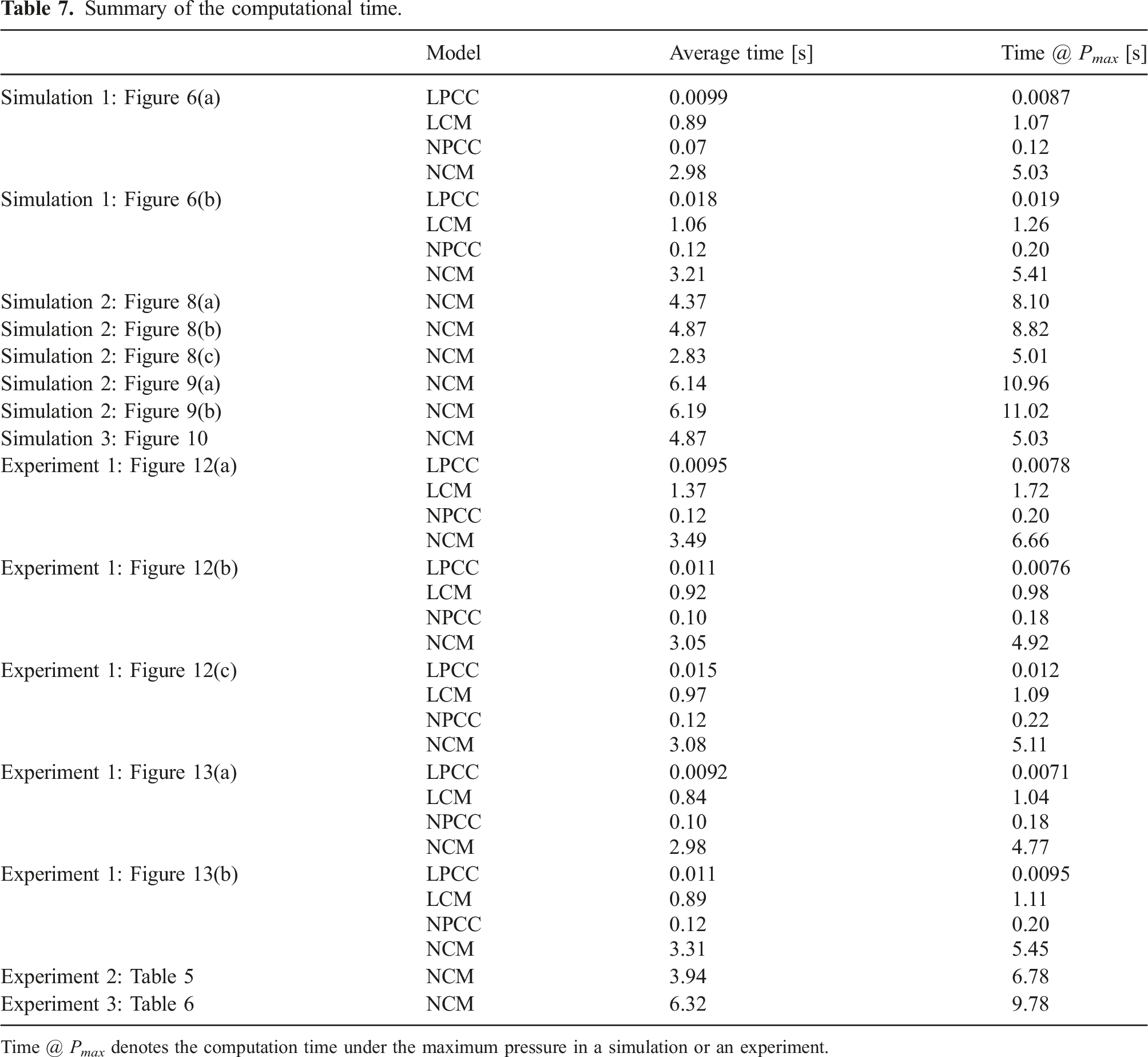
Time @ Pmax denotes the computation time under the maximum pressure in a simulation or an experiment.
The nonlinear compensation in Section 2.3 is comparable to the nonlinear matrix structural analysis in Naselli and Mazzolai (2021), on the other hand, the iterative updates increase the computation complexity (see Table 7). As such, it is also worthy to incorporate the exact hyper-elastic models into the proposed framework (Marechal et al., 2021) to ease the computation. In addition, it is also encouraging to explore the research in the solid mechanics to study the influences of the cross-sectional deformation (Kumar and Mukherjee 2011).
In summary, the proposed stiffness modelling and analysis method can be used to quantitatively assess the stiffness/compliance response of soft robots under different configurations, which may provide new insights to explore on-demand stiffness analysis and optimisation of soft robots with regards to application requirements. Moreover, in serially connected soft robots, the proposed method could be used to optimise the configuration with high stiffness capability along a desired direction.
Supplemental Material
Supplemental Material
Supplemental Material
Footnotes
Declaration of Conflicting Interests
The author(s) declared no potential conflicts of interest with respect to the research, authorship, and/or publication of this article.
Funding
The author(s) disclosed receipt of the following financial support for the research, authorship, and/or publication of this article: This work was supported by the Springboard Award of the Academy of Medical Sciences (grant number: SBF003-1109), the Engineering and Physical Sciences Research Council (grant numbers: EP/R037795/1, EP/S014039/1 and EP/V01062X/1), the Royal Academy of Engineering (grant number: IAPP18-19\264), the UCL Dean’s Prize, UCL Mechanical Engineering, and the China Scholarship Council (CSC).
Supplemental Material
Supplemental material for this article is available online.
Index to multimedia extensions
The multimedia Extensions associated with the paper are listed in Table A1. Multimedia content.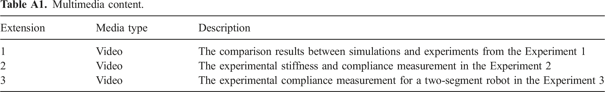
Extension
Media type
Description
1
Video
The comparison results between simulations and experiments from the Experiment 1
2
Video
The experimental stiffness and compliance measurement in the Experiment 2
3
Video
The experimental compliance measurement for a two-segment robot in the Experiment 3
Basics of lie theory
A twist
Considering two screws
More details can refer to Murray et al. (1994); Qiu and Dai (2021).
Transformation matrix in the PCC model
The general form of gi(i+1) based on the PCC model is shown in (43).
Orthonormality of the integrated rotation matrix
As reported in Section 3.3, we used a Fourth-order Runge–Kutta method to achieve numerical integration, with a total discretised number of 50. To show the integration is accurate and feasible maintaining the orthonormality of the integrated rotation matrices, the truncation error is defined in (52) Truncation error of the rotation matrix when using a Fourth-order Runge–Kutta method, when P1 = P2 = 1.5 bar, P3 = P4 = 1.0 bar. (a) The orthonormality error of the integrated rotation matrix at the tip of the soft manipulator when the discretised element number is between 1 and 50. (b) The orthonormality error of the integrated rotation matrix along the manipulator (s ∈ (0, l)) when the discretised number is 50).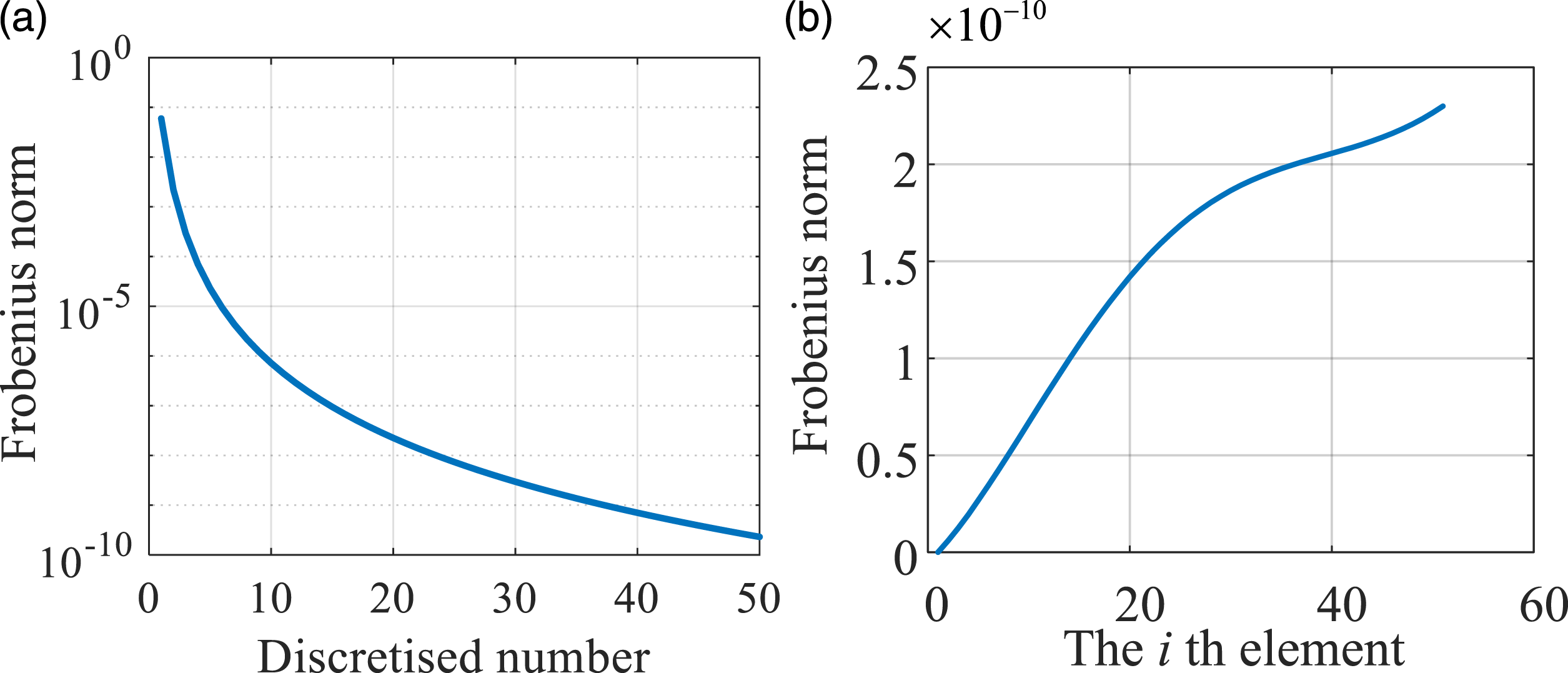
Simulation of the configuration-dependent compliance modelling for a parallel continuum robot
To demonstrate the transferability of our stiffness modelling and analysis framework, we conducted simulations for a parallel continuum robot of a Stewart–Gough configuration (Black et al. 2017). This robot consists of six flexible rods, and its configuration can be varied by controlling the length of each rod. The forward kinematics model used was established based on the Cosserat rod model (Till et al. 2019), and the authors have made their open-source code available on Github under the MIT License, which we incorporated into our framework. Our simulation results demonstrate the effectiveness of our framework in achieving compliance modelling and analysis. It should be noted that the cross-sectional deformation of the rods in this case is negligible, and thus, the LCM of our framework was adopted.
The tip compliance
All stiffness and compliance matrices are expressed in the global frame, and the compliance of the tip is visualised using ellipsoids, as described in Section 2.4. The results of this analysis, which include three different configurations, are presented in Figure A2. Simulation results for the compliance model of a parallel continuum robot of a Stewart–Gough configuration, visualised using compliance ellipsoids when the robot (a) elongates (b) translates (c) bends. The dimension of the compliance ellipsoids is scaled by 250, 60, and 15 for visualisation.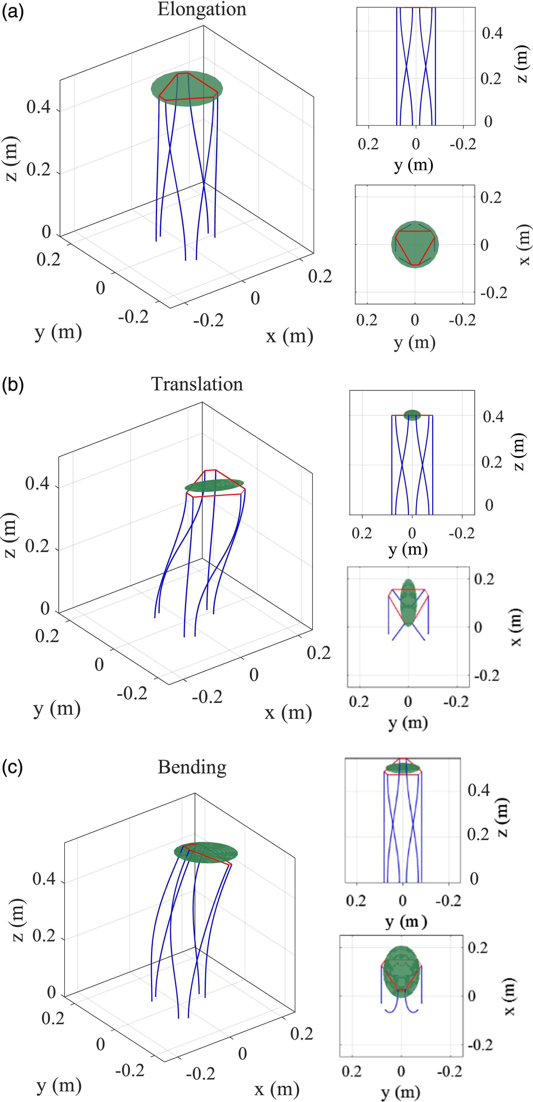
Figure A2(a) shows the computational results when the compliance along the x- and y-axes is isotropic and around 110 times higher than the compliance along the z-axis. Figure A2(b) reports on the results when the robot tip translates to [0.1, 0, 0.4] m while keeping the bending angle at 0°. The overall compliance of the robot increases, and the compliance along the x-axis is about 2 times higher than that along the y-axis. The compliance further increases when the robot bends (see Figure A2(c)), and the compliance along the x- and y-axes becomes more isotropic, which yields a similar tendency with the results from Figure 8(a). As summarised in Table 1, our compliance modelling framework does not require a finite differentiation procedure, compared to other prominent work by, for example, Rucker et al. (2011) and Black et al. (2017).
References
Supplementary Material
Please find the following supplemental material available below.
For Open Access articles published under a Creative Commons License, all supplemental material carries the same license as the article it is associated with.
For non-Open Access articles published, all supplemental material carries a non-exclusive license, and permission requests for re-use of supplemental material or any part of supplemental material shall be sent directly to the copyright owner as specified in the copyright notice associated with the article.