Toward certifiable optimal motion planning for medical steerable needles

Abstract

Medical steerable needles can follow 3D curvilinear trajectories to avoid anatomical obstacles and reach clinically significant targets inside the human body. Automating steerable needle procedures can enable physicians and patients to harness the full potential of steerable needles by maximally leveraging their steerability to safely and accurately reach targets for medical procedures such as biopsies. For the automation of medical procedures to be clinically accepted, it is critical from a patient care, safety, and regulatory perspective to certify the correctness and effectiveness of the planning algorithms involved in procedure automation. In this paper, we take an important step toward creating a certifiable optimal planner for steerable needles. We present an efficient, resolution-complete motion planner for steerable needles based on a novel adaptation of multi-resolution planning. This is the first motion planner for steerable needles that guarantees to compute in finite time an obstacle-avoiding plan (or notify the user that no such plan exists), under clinically appropriate assumptions. Based on this planner, we then develop the first resolution-optimal motion planner for steerable needles that further provides theoretical guarantees on the quality of the computed motion plan, that is, global optimality, in finite time. Compared to state-of-the-art steerable needle motion planners, we demonstrate with clinically realistic simulations that our planners not only provide theoretical guarantees but also have higher success rates, have lower computation times, and result in higher quality plans.

1. Introduction

Steerable needles are highly flexible medical devices able to follow 3D curvilinear trajectories inside the human body, reaching clinically significant targets while safely avoiding critical anatomical structures (Alterovitz et al., 2005; Cowan et al., 2011; Park et al., 2005; Webster et al., 2006). Compared with traditional rigid medical instruments, steerable needles can reduce a patient’s trauma, increase safety, and provide minimally invasive access to previously inaccessible targets. Steerable needles have been considered for a wide range of diagnostic and treatment procedures including biopsy, drug therapy delivery, and radioactive seed implantation for cancer treatment (Abolhassani et al., 2007).

Direct manual control of steerable needles can be unintuitive and impractical for human operators due to the nonholonomic constraints on the needle’s 3D motion and the cluttered nature of anatomical environments. Thus, automation is critical to harnessing the full potential of these needles and enabling physicians to maximally leverage their steerability and ability to accurately and precisely reach targets. To automate steerable needle procedures, physicians first obtain a medical image (such as a computed tomography (CT) or magnetic resonance imaging (MRI) scan) of the relevant anatomy, from which we can segment (manually or automatically) the relevant anatomy, including the target to reach and obstacles to avoid. The next key ingredient to the automation of steerable needle procedures is motion planning, which requires computing feasible motions to steer the needle safely around the anatomical obstacles and to the target. Examples of scenarios of lung and liver biopsies are shown in Figure 1 (top).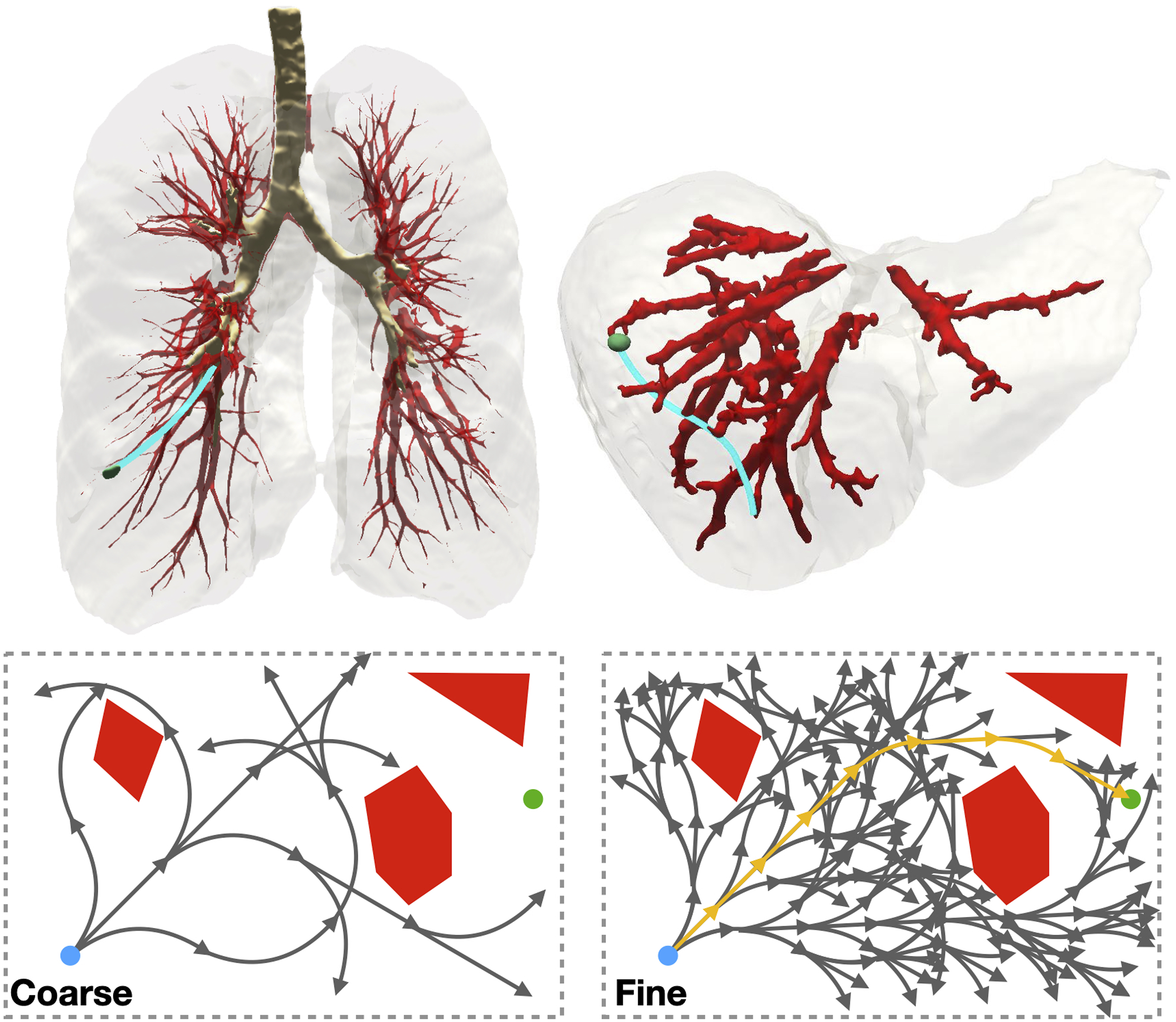

Figure 1.

Top left: A medical steerable needle (cyan) is used to reach a nodule (green) in the lung parenchyma for biopsy or cancer treatment while avoiding critical anatomical structures such as the bronchial tubes (brown) and major blood vessels (red). Top right: A medical steerable needle (cyan) is used to reach a nodule (green) in the liver tissue while avoiding major blood vessels (red). Bottom: Our resolution-complete motion planner uses search trees built using different resolutions, illustrated here in 2D. A valid motion plan goes from the start configuration (blue dot) to the goal point (green dot), while avoiding obstacles (red) and satisfying kinematic constraints. The left search tree uses a coarse resolution and fails to find a plan while the right one uses a finer resolution and successfully generates a motion plan (yellow).

For the automation of medical procedures to be clinically accepted, it is critical from a patient care, safety, and regulatory perspective to certify the correctness and effectiveness of the algorithms involved in procedure automation. To this end, a motion planner should first guarantee that it will compute a solution, when one exists, in finite time, or notify the user that no solution exists. Moreover, the computed solution should strive to maximize patient safety, which can be quantified using metrics such as minimizing trajectory length (Favaro et al., 2018), maximizing clearance from obstacles (Agarwal et al., 2018; Kuntz et al., 2015; Strub and Gammell, 2021; Wein et al., 2008), and minimizing damage to sensitive tissue (Bentley et al., 2021; Fu et al., 2018). Thus, a motion planner for steerable needles should be complete, that is, find a solution plan in a finite number of steps, if one exists, and ideally should be optimal, that is, ensure that the returned plan has a cost (for a given cost metric) that is close to the global optimum. Unfortunately, no previously developed motion planner for steerable needles offers a formal guarantee on completeness, let alone optimality.

Although various motion planners have been proposed for steerable needles, those planners do not have theoretical guarantees for either returning a solution (Duindam et al., 2010; Favaro et al., 2018; Hauser et al., 2009; Patil et al., 2014; Pinzi et al., 2021; Seiler et al., 2012; Van Den Berg et al., 2010; Xu et al., 2008) or returning a solution that terminates within a clinically reasonable distance of the target (Liu et al., 2016) when a solution exists. Some prior motion planners for steerable needles do aim to optimize motion plan cost but they lack global optimality guarantees (Favaro et al., 2018; Favaro et al., 2021; Liu et al., 2016; Pinzi et al., 2019). Some sampling-based planners are known to be both complete and optimal, albeit those properties are usually proven only for an asymptotic regime where the number of samples tends to infinity (Hauser and Zhou, 2016; Karaman and Frazzoli, 2011; Kleinbort et al., 2018, 2020; LaValle and Kuffner Jr, 2001; Li et al., 2016; Salzman and Halperin, 2015; Solovey et al., 2020; Sun et al., 2015). Thus, it is unclear what should be the number of samples necessary to achieve those guarantees in practice. Recent work has developed optimality guarantees for finite sampling, although those results cannot be currently applied to steerable needles as they deal with holonomic systems (Dayan et al., 2021; Tsao et al., 2020).

Providing completeness and optimality guarantees for a steerable needle motion planner is challenging in part because motion planning for steerable needles in 3D with curvature constraints is at least NP-hard (Kirkpatrick et al., 2011; Solovey, 2020). This challenge inspires us to consider variants of completeness or optimality relevant to medical applications. Some variants that only offer asymptotic guarantees, such as probabilistic completeness and asymptotic optimality (LaValle, 2006), are not useful for needle steering since these guarantees only hold as computation time increases to infinity, but medical applications typically require guaranteeing the planner’s behavior within a finite time.

In this paper, we focus on specific types of guarantees relevant to real-world medical applications: resolution completeness (LaValle, 2006) and resolution optimality (Barraquand and Latombe, 1993; Pivtoraiko et al., 2009). Generally speaking, a resolution characterizes the discretization of some space (e.g., state space, configuration space, action space, and time). An algorithm is resolution complete if there exists a fine-enough resolution with which the algorithm finds a plan in finite time when a qualified solution exists, and otherwise correctly returns that no such plan exists. An algorithm is resolution optimal if it is resolution complete and if, when it does return a motion plan, the plan’s cost is guaranteed to be within a desired approximation factor of the cost of a globally optimal qualified motion plan. We illustrate at the bottom of Figure 1 an example showing searches with different resolutions for needle steering.

1.1. Contribution

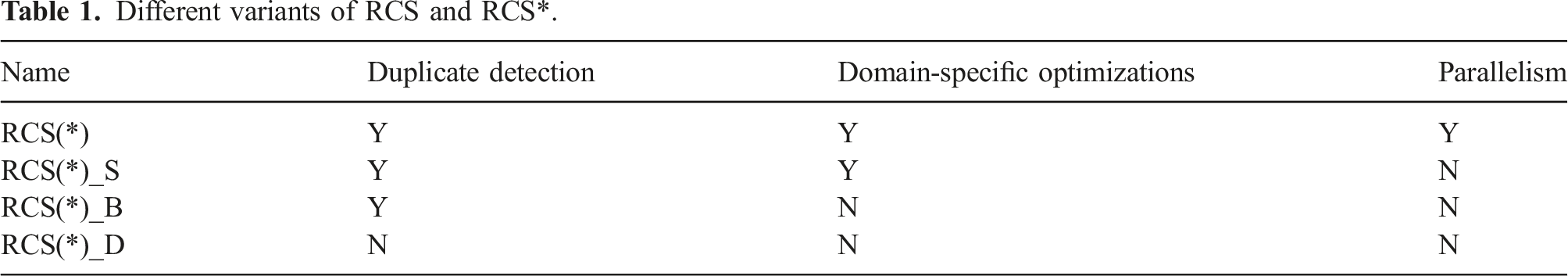
In this paper, we first present Resolution-Complete Search (RCS), an efficient, resolution-complete motion planner for steerable needles based on a novel adaptation of multi-resolution planning. RCS is resolution complete, which means that under some mild assumptions on the system and the solution (detailed in Section 5), the planner, in finite time, is guaranteed to find a motion plan as long as the problem admits a qualified solution. We then describe an extension of RCS, called RCS*, that achieves resolution optimality. In particular, RCS* explores the needle’s state space in an A*-like fashion, with cost-aware duplicate pruning while incorporating motion plan cost tracking and a heuristic function to improve efficiency.

Our overall contributions include (i) carefully defining the motion primitives (Frazzoli et al., 2002) used by our planners, which are specifically tailored to our domain of 3D steerable needles (Section 4.1.1); (ii) introducing a set of domain-specific optimizations that improve the efficiency of the algorithm while maintaining resolution completeness and resolution optimality (Section 4.3); and (iii) providing a proof to show the resolution completeness and optimality of our methods (Section 5).

We demonstrate the performance of our planners in two clinically realistic scenarios where the needle should reach a target while safely avoiding obstacles (e.g., blood vessels). In the setting of (i) lung biopsy, the needle is deployed through a bronchoscope and must steer through the lung parenchyma (the tissue of the lung outside the bronchial tubes) and in the setting of (ii) liver biopsy, the needle is deployed into the liver through its anterior surface and must steer through the liver tissue. We compare in simulation our planner with several other steerable needle planners and demonstrate experimentally that RCS and RCS* outperform the state-of-the-art in terms of computation time, success rate, and plan quality.

This work is the integration and extension of two conference papers (Fu et al., 2021b, 2022) where we introduced RCS and RCS*, respectively. The main changes in the current version from the previous conference papers are (i) full proofs for resolution optimality that were previously given as sketches, (ii) new experiments for a liver biopsy scenario, and (iii) an extended set of experimental results, including an ablation study on the algorithms’ parameters.

2. Related work

Steerable needles have many different designs, including bevel-tip flexible needles (Cowan et al., 2011; Webster et al., 2006), symmetric-tip needles (DiMaio and Salcudean, 2003), needles with curved stylet tips (Okazawa et al., 2005), needles with tendon-actuated tips (Qi et al., 2014), programmable bevel-tip needles (Ko et al., 2011; Secoli and Rodriguez Y Baena, 2016), and fracture-directed waterjet steerable needles (Babaiasl et al., 2020). In this paper, we focus on bevel-tip flexible needles but our approach can be easily applied to any mechanical design as long as the major kinematic constraint to consider is the curvature of the needle trajectory.

2.1. Motion planning for steerable needles

Early work studied planning and control for steerable needles in the 2D plane (Alterovitz et al., 2007; Asadian et al., 2011; Bernardes et al., 2012; Reed et al., 2011). To fully utilize the capability of steerable needles, later work began to focus more on needle steering in 3D environments. Duindam et al. (2010) used inverse kinematics for planning but the planner was tested only with simple geometrically shaped obstacles and provides no theoretical guarantees.

Other planners built upon the probabilistic completeness guarantees of sampling-based methods such as the Rapidly-exploring Random Tree (RRT) (LaValle and Kuffner Jr, 2001). For example, Xu et al. (2008) used an RRT variant for needle steering (although having slow running times when compared to alternatives we will mention shortly) and Patil et al. (2014) developed an RRT-based needle planner that guides the tree expansion by sampling in the 3D workspace (instead of the configuration space). Sampling in a lower-dimension space and their customized distance function made the planner work efficiently in many practical cases, but this also invalidated the probabilistic-completeness guarantee of RRT (Kleinbort et al., 2020; LaValle and Kuffner Jr, 2001). Sun et al. (2015) proposed a needle planner that builds multiple RRTs, which is asymptotically optimal only when the number of trees tends to infinity.

To avoid dealing with curvature constraints directly in the RRT algorithms, there are also hybrid methods that combine sampling and other techniques. Favaro et al. (2018) proposed a method based on RRT* (Karaman and Frazzoli, 2011) that builds a tree embedded in the 3D workspace to generate candidate plans of low cost, followed by a smoothing step to account for the curvature constraint. This was later extended into another hybrid method that combines sampling, optimization, and search (Favaro et al., 2021). However, such a decoupling does not allow to guarantee asymptotic optimality (Karaman and Frazzoli, 2011; Solovey et al., 2020).

Liu et al. (2016) proposed the Adaptive Fractal Tree (AFT) for needle steering and used a Graphics Processing Unit (GPU) to further speed up their algorithm. The method uses a greedy approach for path refinement—it iteratively uses the lowest-cost path in the previous iteration for plan refinement. However, expanding the best path of a coarse resolution does not necessarily lead to a best path of a finer resolution. Furthermore, the authors use a cost function consisting of three factors, only one of which is the distance to the goal, also known as the targeting error. Thus, when provided with a required targeting error, paths produced by the method are not guaranteed to adhere to this constraint since the targeting error may be sacrificed for a better cost for the other two terms. Pinzi et al. (2019) later extended AFT to account for goal orientation constraints.

Other methods focus on accounting for uncertainties during needle insertion but do not account for completeness (Hauser et al., 2009; Pinzi et al., 2021; Seiler et al., 2012; Van Den Berg et al., 2010). To summarize, to the best of the authors’ knowledge, none of the existing steerable needle planners provide provable guarantees on the planner’s completeness.

2.2. Resolution-complete motion planners

Generally speaking, an algorithm is resolution complete if it generates a plan to the goal whenever a solution exists at the maximal resolution and returns failure otherwise (Barraquand and Latombe, 1991). This property guarantees that given a predefined maximal resolution, the algorithm terminates in finite time and provides a deterministic result.

Barraquand and Latombe (1993) proposed a planner for single/multi-body mobile robots with nonholonomic constraints. They formally proved the planner is guaranteed to generate a solution path when the discretization of the search parameters is fine enough. This approach was later extended by Lindemann and LaValle (2006) to suggest a multi-resolution approach for 2D car-like robots. Both these works (Barraquand and Latombe, 1993; Lindemann and LaValle, 2006) serve as the algorithmic foundations of the planner we present in this paper.

Sampling-based planners (such as RRT) typically ensure probabilistic completeness (i.e., such a planner is guaranteed to find a solution, if one exists, with probability one when given infinite time). However, they can also be used to build resolution-complete planners given some mild assumptions on the minimal motion that the system can perform. Cheng and LaValle (2002) proposed a resolution-complete version of RRT for systems that satisfy the Lipschitz condition. Yershov and LaValle (2010) formally analyzed the system conditions for the existence of resolution-complete planners. Kleinbort et al. (2018) later analyzed the assumptions for RRT’s probabilistic completeness in kinodynamic planning. However, their analysis can be adapted to resolution-completeness guarantees.

2.3. Resolution-optimal motion planners

Resolution optimality earned little attention, possibly due to being rather complex to analyze mathematically, particularly for nonholonomic systems. Consequently, many planners developed for nonholonomic systems focus on asymptotic optimality instead (Gammell and Strub, 2021; Hauser and Zhou, 2016; Li et al., 2016; Shome and Kavraki, 2021).

The previously mentioned method of Barraquand and Latombe (1993) for resolution-complete planning with nonholonomic constraints is optimal with respect to the number of reverse maneuvers in the plan. Pivtoraiko et al. (2009) proposed the idea of motion planning using state lattices for field robots. Their state lattices planner is resolution optimal since the search is optimal for a graph of some resolution and the discrete state grid approximates the continuous space as resolution increases. Ljungqvist et al. (2017) later extended Pivtoraiko et al. (2009) for a general two-trailer system in 2D. They used a two-point boundary value problem (2pBVP) solver to generate a set of motion primitives connecting 2D grid points.

The aforementioned planners can be used to plan for 2D nonholonomic robots, but none account explicitly for the challenges of planning with curvature constraints in 3D. (The latter case is particularly challenging not only because of the higher dimensional search space but also because of the absence of boundary-value solvers.) Additionally, these planners are designed for large-scale workspaces (where the minimum radius of curvature is relatively small compared to the scale of the workspace), making them unsuitable for tasks where a high level of precision is required, such as for steerable needles.

3. Problem definition

In this work, we consider steerable needles that operate in a 3D workspace $\mathcal{W}\in {\mathbb{R}}^3$ , which is cluttered with obstacles ${\mathcal{W}}_{\text{obs}}\subset \mathcal{W}$ . We define the configuration space (or C-space) of the steerable needle as $\mathcal{X}\subset \mathcal{S}\mathcal{E}\left(3\right)$ . Each configuration $\mathbf{x}=\left(p,q\right)\in \mathcal{X}$ uniquely defines the pose (i.e., position $p\in {\mathbb{R}}^3$ and orientation $q\in \mathcal{S}\mathcal{O}\left(3\right)$ ) of the needle tip. We define a projection function $\text{Proj}(\cdot ):\mathcal{X}\to \mathcal{W}$ that projects configurations to points in the workspace, that is, Proj(x) = p. A configuration x is collision free if $\text{Proj}\left(\mathbf{x}\right)\notin {\mathcal{W}}_{\text{obs}}$ , and is in collision otherwise. The union of all collision-free configurations is denoted as ${\mathcal{X}}_{\text{free}}$ . We make the common assumption that the steerable needle is sufficiently flexible so the needle shaft moves along the trajectory created by its tip while the lateral motions are negligible. Thus, a motion plan of the needle can be uniquely defined as a trajectory $\sigma :\left[0,\ell \right]\to \mathcal{X}$ , where ℓ is the length of the trajectory defined in the 3D Euclidean distance space. Such a motion plan σ is collision free if all configurations along the trajectory are collision-free, namely, $\forall s\in \left[0,\ell \right],\sigma \left(s\right)\in {\mathcal{X}}_{\text{free}}$ .

We also need to consider the kinematics of the steerable needle. We specifically consider steerable needles that are highly flexible and have an asymmetric tip (e.g., a bevel) (Alterovitz et al., 2005, Cowan et al., 2011, Park et al., 2005, and Webster et al., 2006); the asymmetric tip exerts asymmetric forces on the tissue in front of the needle tip, and the high flexibility enables the needle to curve substantially at maximum curvature κ_max as it moves through the tissue. Furthermore, rotating the needle axially at its base changes the direction of the needle’s asymmetric tip, enabling the needle to change its direction of steering. See Figure 2 for an illustration.

Figure 2.

The kinematics of a bevel-tip steerable needle. The needle can be inserted (characterized by ℓ) and axially rotated at its base (characterized by θ).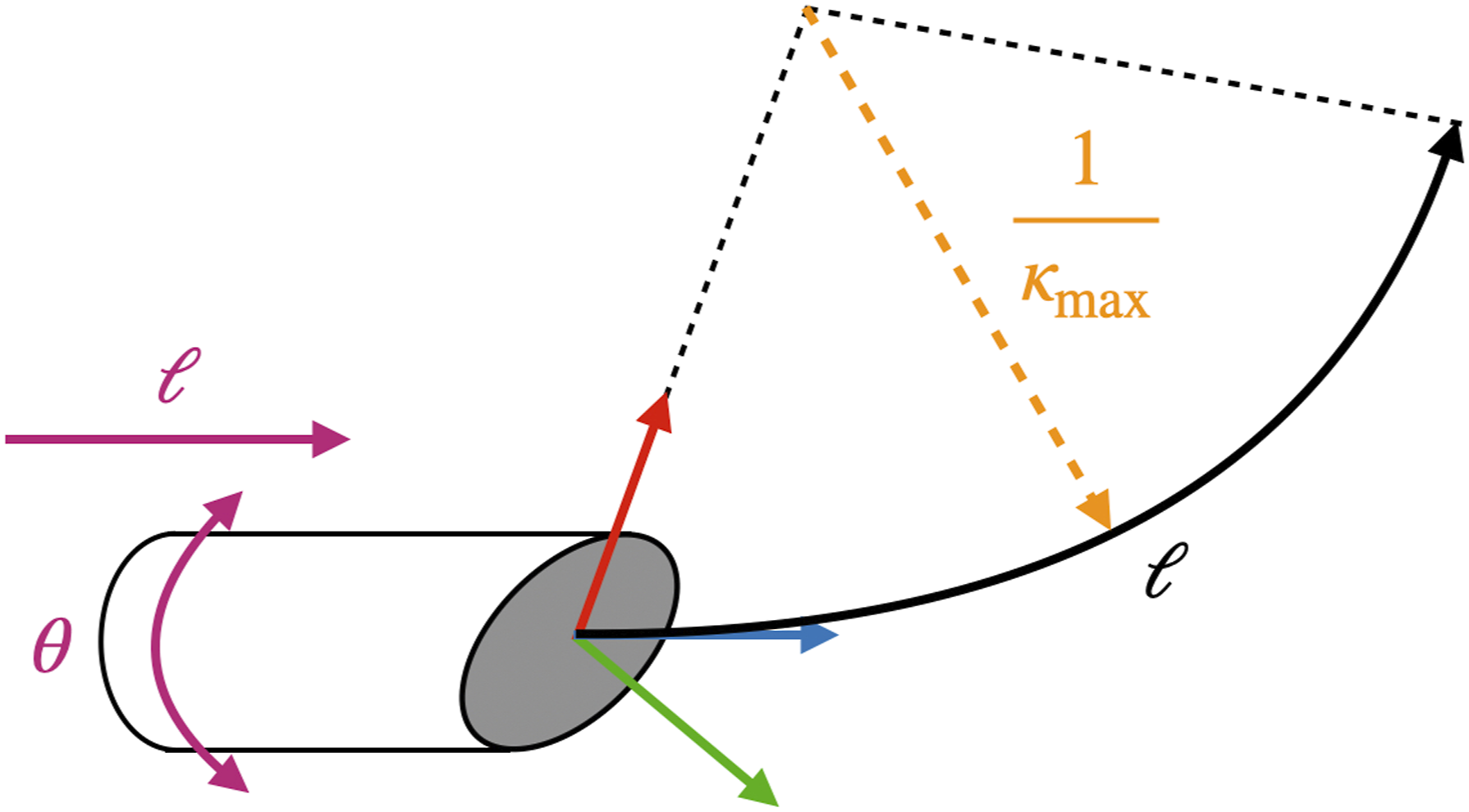

We say a motion plan is (kinematically) feasible if it never exceeds the maximum curvature κ_max. A valid motion plan for the needle is both collision-free and feasible. We also assume there exists a resolution describing the smallest interval or precision of the achievable motions, which may be limited by the physical system’s hardware (e.g., motor, encoders, and controller) and its interaction with the environment. For the steerable needle application in this paper, we determine this finest resolution by considering the hardware’s ability to measurably change the steerable needle tip’s position and orientation in tissue, which includes parameters such as the minimum insertion distance and rotational direction change per controller time step, as defined in Section 4. Considering real-world effects such as torsional wind-up of the needle shaft during actuation, the control resolution of the needle tip is coarser than the control resolution of the needle base where motors directly apply controls. Thus, we are not using minimal motions of the motors. Instead, we consider the minimal motions the tip of the needle can perform. We assume there exists a lower-level controller capable of controlling the tip to the desired pose, as is common in needle-steering systems (Ertop et al., 2020; Rucker et al., 2013).

We are now ready to state two different problems considered in this work. The first problem calls for computing a valid motion plan for a given case while the second problem is formulated as an optimization problem with respect to the cost of a motion plan.

3.1. Steerable needle motion planning problem

Problem 1

A steerable needle motion planning problem is defined as the tuple $\mathrm{\Delta }=\left(\mathcal{X},{\mathcal{W}}_{\text{obs}},{\mathbf{x}}_{\text{start}},p_{\text{goal}},\tau ,{\ell }_{\max },{\kappa }_{\max }\right)$ , where ${\mathcal{W}}_{\text{obs}}$ is the obstacle set, x_start is the start configuration, $p_{\text{goal}}\in \mathcal{W}$ is the goal point, τ > 0 is the goal tolerance, ℓ_max > 0 is the maximum insertion length, and κ_max > 0 is the maximum curvature. The problem calls for computing a motion plan $\sigma :\left[0,\ell \right]\to \mathcal{X}$ subject to:

   (i) σ is valid,

   (ii) σ(0) = x_start,

   (iii) trajectory length ℓ ≤ ℓ_max,

   (iv) ‖Proj(σ(ℓ)) − p_goal‖₂ ≤ τ.

As we show in our discussion (Section 5), for any given instance of Problem 1, under some mild assumptions, there exists some fine-enough resolution R_min = (δℓ_min, δθ_min) (corresponding to the needle’s insertion and axial rotation, respectively) for which our proposed planner, RCS, is guaranteed to find a solution in finite time (when one exists) or to indicate that no solution exists.

3.2. Optimal steerable needle motion planning problem

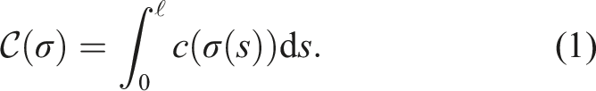
To evaluate the quality of a motion plan, we consider a configuration-based cost function $c:\mathcal{X}\to \mathbb{R}$ . We require c to be well behaved (formally defined in Section 5), which includes being Lipschitz continuous and bounded within [c_min, c_max]. We define the cost of a motion plan as the integral of the configuration-based cost function along a given trajectory σ, that is,

$\mathcal{C}\left(\sigma \right)={\int }_0^{\ell }c\left(\sigma \left(s\right)\right)\mathrm{d}s.$

(1)

If a cost function satisfies the above form, we say it is an integrated cost function. This definition captures a variety of cost functions, including trajectory length and integrating over a cost map derived from medical images.

Problem 2

An optimal steerable needle motion planning problem is defined as an optimization problem, denoted by a tuple ${\mathrm{\Delta }}^{*}=\left(\mathrm{\Delta },\mathcal{C}\right)$ , where Δ is a steerable needle motion planning problem defined in Problem 1 and $\mathcal{C}$ is an integrated cost function. The current problem calls for computing an optimal motion plan

${\sigma }^{*}={\mathrm{argmin}}_{\sigma }\mathcal{C}\left(\sigma \right),$

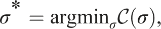
subject to the same four conditions as in Problem 1.

Similarly, we will show in Section 5 that for any given instance of Problem 2, under some mild assumptions, there exists a fine-enough cutoff resolution R_min = (δℓ_min, δθ_min) for which our proposed planner, RCS*, is guaranteed to return a motion plan with a cost to be within a desired approximation factor of a globally optimal qualified motion plan in finite time (if any qualified motion plan exists), or indicate that no qualified motion plan exists.

4. Method

In this section, we first describe the resolution-complete needle planner RCS in Section 4.1. We then provide in Section 4.2 a resolution-optimal extension called RCS*. Finally in Section 4.3, we highlight a set of optimizations that improve the efficiency of both RCS and RCS*.

4.1. Resolution Complete Search

Given our motion-planning problem, our needle planner builds a search tree $\mathcal{T}=\left(\mathcal{V},\mathcal{E}\right)$ embedded in the C-space with x_start as its root. Each node $v\in \mathcal{V}$ is associated with a configuration ${\mathbf{x}}_v\in \mathcal{X}$ , and each edge $e=\left(v,u\right)\in \mathcal{E}$ represents the transition from x _v to x _u . To expand a node $v\in \mathcal{V}$ , we construct new nodes (children of v) with motion primitives (to be explained shortly in Section 4.1.1), which are predefined feasible motions. A child node v_child is accepted and added to the search tree if the trajectory from v to v_child is collision-free and v_child is valid (will be detailed in Section 4.1.3). The search tree grows until there is some node v with configuration x _v whose tip is inside the τ-neighborhood of p_goal (condition (ii) in Problem 1).

A key aspect of our search method (which is similar in nature to other search-based planners like Lindemann and LaValle (2006)) is to use a set of motion primitives defined using multiple resolutions. Instead of expanding each node in our search tree using the entire set of motion primitives, we start with coarse motion primitives and use finer motion primitives as the search progresses. Thus, we start (Section 4.1.1) by describing the parameters required to define a motion primitive. After that, we continue (Section 4.1.2) to detail a hierarchy of motion primitives together with an ordering that will be used in our search algorithm. We then describe our search algorithm in detail (Section 4.1.3) and elaborate on the method we use to handle “similar” states, also known as duplicate detection (Du et al., 2019) (Section 4.1.4).

4.1.1. Motion primitives

Motion primitives, introduced by Frazzoli et al. (2002), have been used in many motion planners (Islam et al., 2019, 2020; Lindemann and LaValle, 2006; Ljungqvist et al., 2017; Pivtoraiko and Kelly, 2011). In our setting, the motion primitives are a set of predefined kinematically feasible local motions. Roughly speaking, a motion primitive defines with what curvature the needle curves, how far the needle steers, and in which direction (see Figure 3). Since for each motion primitive, the curvature κ is explicitly defined, a motion primitive is guaranteed to be kinematically feasible as long as κ ≤ κ_max.

Figure 3.

A motion primitive is a circular arc defined as 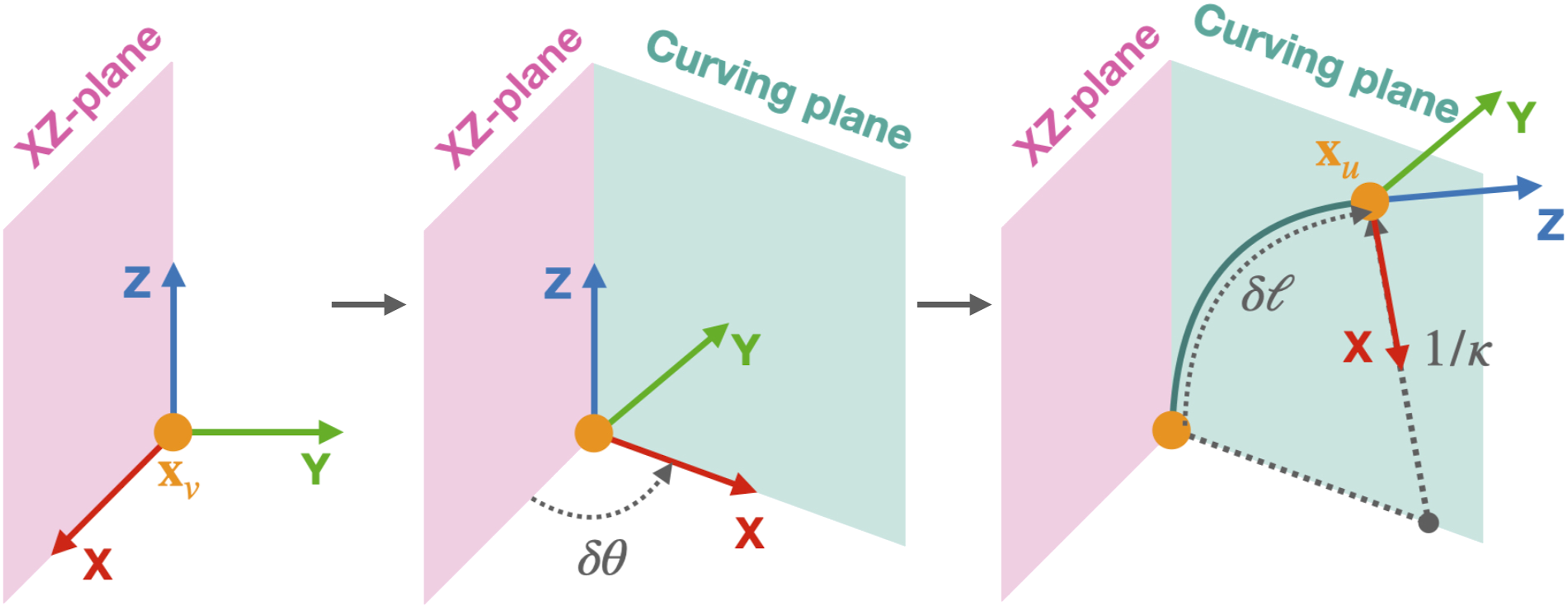$\mathcal{M}=\left(\kappa ,\delta \ell ,\delta \theta \right)$ . The circular arc (dark green) lies in the curving plane (light green) that contains the Z-axis (blue) at the start configuration x _v . κ is the curvature of the arc, δθ is the angle between the curving plane and the XZ-plane, and δℓ is the length of the arc. The figures show step-by-step how the child configuration ${\mathbf{x}}_u={\mathbf{x}}_v\oplus \mathcal{M}$ is generated.

More formally, to steer from configuration x _v , a motion primitive is defined as a three-tuple $\mathcal{M}=\left(\kappa ,\delta \ell ,\delta \theta \right)$ , where κ ∈ [0, κ_max] is the curvature, δℓ > 0 is the length of the circular arc, and $\delta \theta \in [\mathrm{0,2}\pi )$ is the angle between the curving plane and the XZ-plane of x _v (see Figure 3). Thus, the action space (or motion space) can be defined as $\mathcal{A}\subset {\mathbb{R}}^3$ , which is the set of all motion primitives. We use ${\mathbf{x}}_u={\mathbf{x}}_v\oplus \mathcal{M}$ to denote the operation of extending x _v with motion primitive $\mathcal{M}$ and obtaining the resultant configuration x _u . See Figure 3 for a step-by-step determination of x _u . In the context of a search tree, by a slight abuse of notation, $u=v\oplus \mathcal{M}$ denotes the resultant node u, obtained by extending node v with the motion primitive $\mathcal{M}$ . We call $\mathcal{M}$ the extending primitive of node u.

Using motion primitives allows pre-computing intermediate configurations and thus saving computation efforts during planning by transforming these configurations to the frame defined by x _v . Since the trajectory produced with one motion primitive is a circular arc, it is possible to densely interpolate the trajectory for collision-checking purposes.

In the following sections, we show how δℓ and δθ are gradually refined by the algorithm. In contrast, we keep a fixed set of curvatures, {0, κ_max}, for all motion primitives. As we will see (Section 5), this does not hinder the guarantees provided by our approach. Moreover, as we demonstrate in our experiments (Section 6), these primitives, coupled with our planners, allow us to efficiently compute paths for non-trivial instances where other planners fail.

4.1.2. Motion primitive hierarchy

Our algorithm uses a sequence of motion primitives, whose resolution changes from coarse to fine. The coarsest motion primitives are defined by parameters δℓ_max and δθ_max. In our implementation and examples (e.g., Figure 4), we have that δθ_max = π/2 and δℓ_max > 0 is a user-given parameter.

Figure 4.

Visualization of length and angle levels. Left: Visualization of length levels. Smaller node sizes correspond to higher length levels. The first length level (l _ℓ = 0) corresponds to motion primitives of maximal length (δℓ_max). As l _ℓ increases, the resolution of length becomes higher. The gray spheres show the lengths at corresponding length levels while the white spheres show the lengths that have been explored at a smaller level. The gray arrows illustrate how motion primitives with the first 4 length levels are generated during refinement. Right: Visualization of angle levels. Nodes with angle levels 0, 1, and 2 are shown in red, yellow, and blue, respectively. The first angle level (l _θ = 0) corresponds to motion primitives of δθ = {0, π/2, π, 3π/2}. As l _θ increases, the resolution of orientation becomes higher. The circular arrows illustrate how nodes with the first three angle levels are generated during refinement. Middle: 3D visualization of length and angle levels.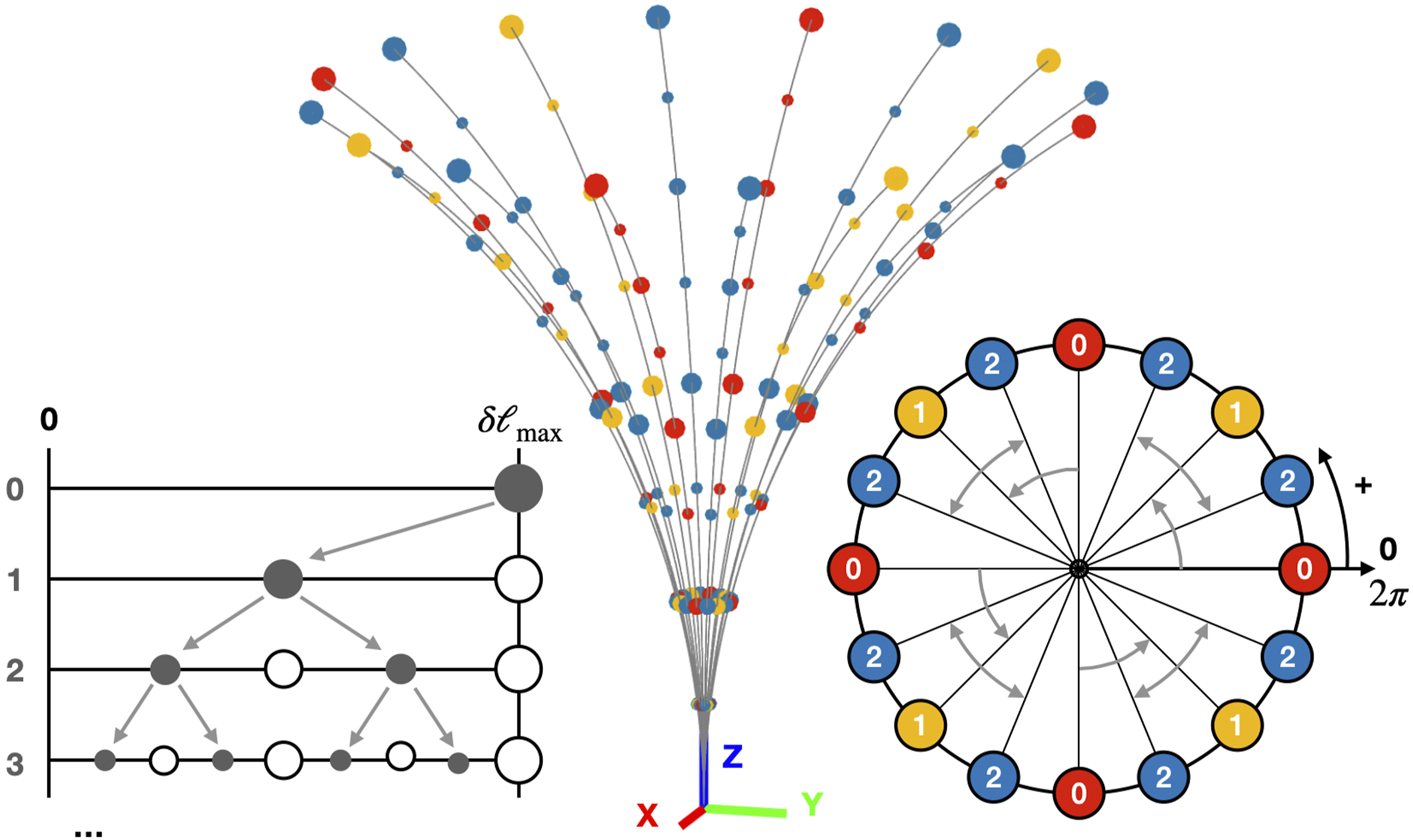

Since $\delta \theta \in [\mathrm{0,2}\pi )$ and δθ_max = π/2, there exist four orientations (δθ ∈ {0, π/2, π, 3π/2}) that have the coarsest orientation (see Figure 4). There exists only one coarsest length, which is δℓ_max, since path length is accumulated when we expand a node. To characterize how fine the resolution of a motion primitive $\mathcal{M}=\left(\kappa ,\delta \ell ,\delta \theta \right)$ is, we define the notions of length level l _ℓ and angle level l _θ . More formally,

$\begin{array}{cc}{l}_{\ell }\left(\mathcal{M}\right)& =\min \left\{l\in \mathbb{Z} \mathbb{|} l\ge 0,\text{MOD}\left(\delta \ell ,2^{-l}\cdot \delta {\ell }_{\max }\right)=0\right\},\\ l_{\theta }\left(\mathcal{M}\right)& =\min \left\{l\in \mathbb{Z} \mathbb{|} l\ge 0,\text{MOD}\left(\delta \theta ,2^{-l}\cdot \delta {\theta }_{\max }\right)=0\right\},\end{array}$

where MOD(·) is the modulo operation.

For a motion primitive $\mathcal{M}=\left(\kappa ,\delta \ell ,\delta \theta \right)$ , we refine the resolution of both the insertion δℓ and the orientation δθ. The new motion primitives constructed by refining δℓ are:

${\mathcal{M}}_{\ell \pm }=\left(\kappa ,\delta \ell \pm 2^{-\left(l_{\ell }\left(\mathcal{M}\right)+1\right)}\cdot \delta {\ell }_{\max },\delta \theta \right).$

(2)

Similarly, the motion primitives constructed by refining δθ are:

${\mathcal{M}}_{\theta \pm }=\left(\kappa ,\delta \ell ,\delta \theta \pm 2^{-\left(l_{\theta }\left(\mathcal{M}\right)+1\right)}\cdot \delta {\theta }_{\max }\right).$

(3)

It is straightforward to see that the refined motion primitives ${\mathcal{M}}_{\ell -}$ and ${\mathcal{M}}_{\ell +}$ both have a length level of $l_{\ell }\left(\mathcal{M}\right)+1$ and the refined motion primitives ${\mathcal{M}}_{\theta -}$ and ${\mathcal{M}}_{\theta +}$ both have an angle level of $l_{\theta }\left(\mathcal{M}\right)+1$ (see Figure 4).

Note that when refining a motion primitive with $l_{\ell }\left(\mathcal{M}\right)=0$ (resp. $l_{\theta }\left(\mathcal{M}\right)=0$ ), we ignore ${\mathcal{M}}_{\ell +}$ (resp. ${\mathcal{M}}_{\theta -}$ ) as they both exceed the range of exploration.

Similar to Lindemann and LaValle (2006), our search algorithm expands nodes according to a node’s rank. Rank captures both the depth of a node in the search tree and the fineness of resolution along the branch connecting the node from the root. We define the rank of the root node to be zero, the rank of any other node v is recursively defined as:

$\text{Rank}\left(v\right)=\text{Rank}\left(v.\text{parent}\right)+l_{\ell }\left({\mathcal{M}}_v\right)+l_{\theta }\left({\mathcal{M}}_v\right)+1.$

(4)

For a visualization, see Figures 4 and 5.

Figure 5.

Nodes of the first four ranks. We use motion primitives with κ = 0 (straight lines) and κ = κ_max (arcs with maximum curvature).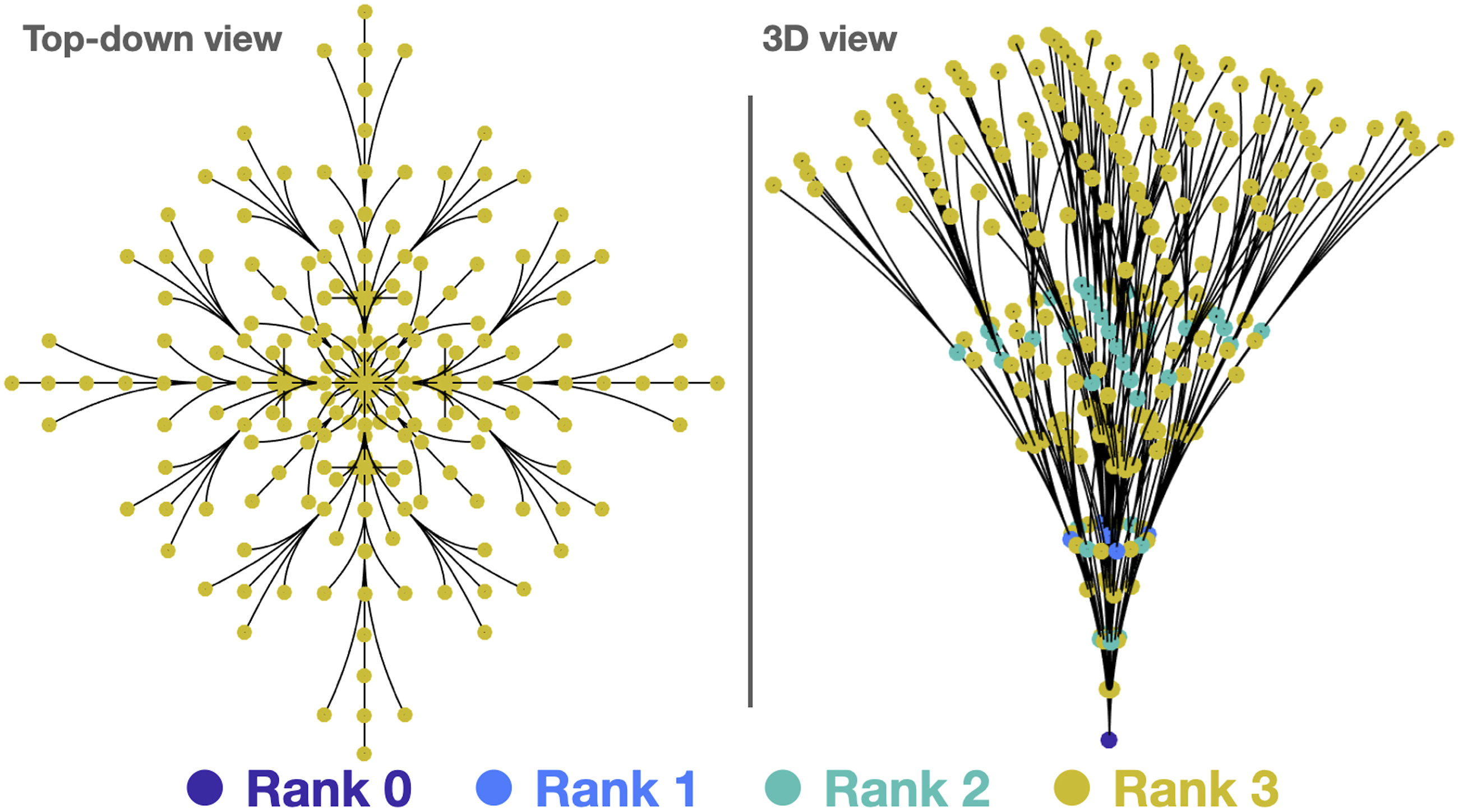

4.1.3. Algorithm description

We run an A*-like search (Hart et al., 1968) where nodes are ordered according to their rank (equation (4)). A distinctive feature from (vanilla) A* is that when we expand a node, we also increase the resolution of the motion primitives used to expand its parent and add nodes using these finer motion primitives to the search’s priority queue. The rest of this section formalizes this idea.

Alg. 1 shows the pseudocode of our RCS needle planner. We first initialize the coarsest orientations and the curvature set (Alg. 1, line 1), and then initialize the OPEN list and CLOSED set (Alg. 1, line 3). The search algorithm then iteratively extracts nodes from the OPEN list (Alg. 1, line 5), where nodes are ordered in a monotonically non-decreasing order according to their rank.

Algorithm 1 ResolutionCompleteSearch (RCS)

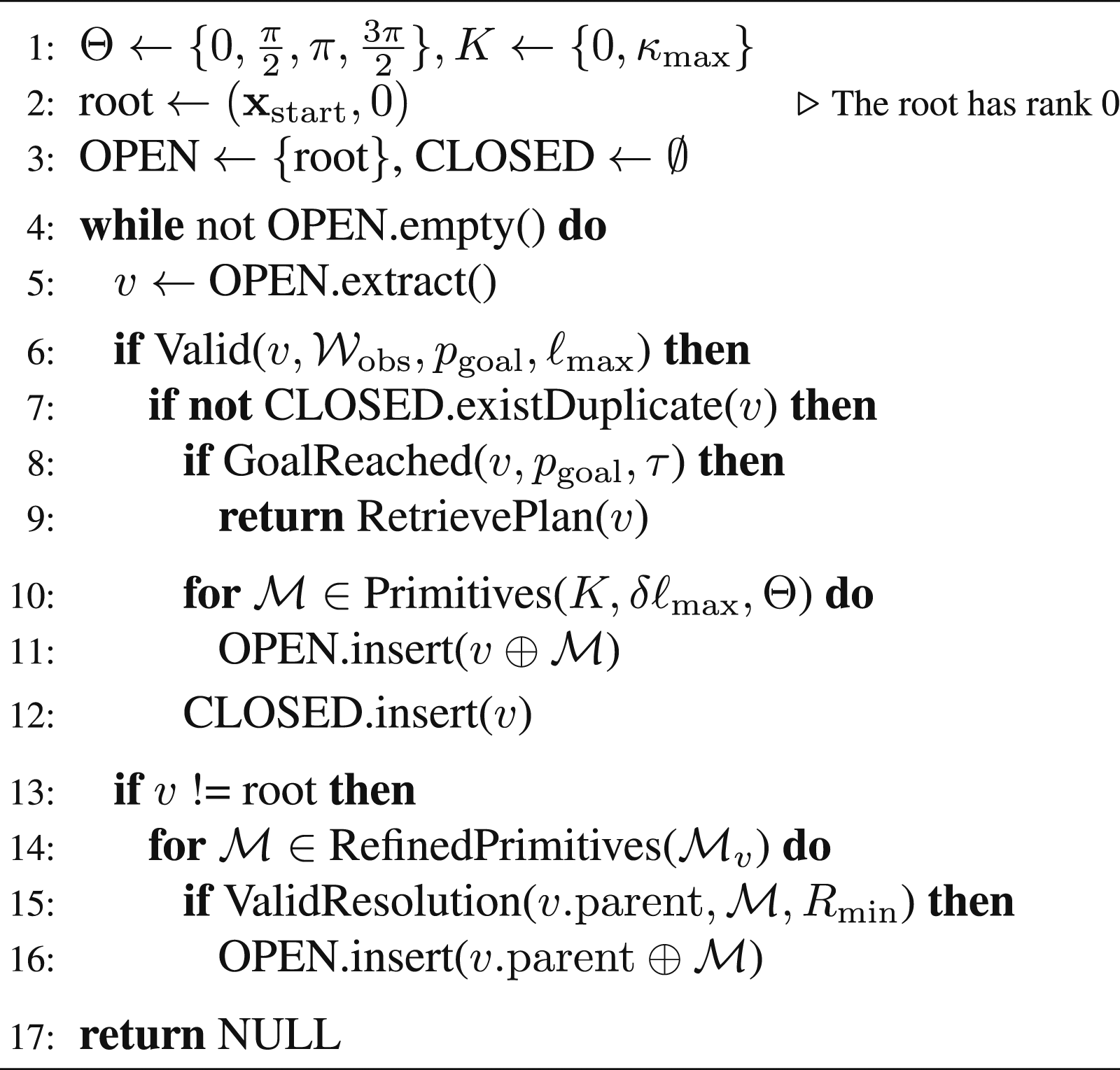
Only at this point (Alg. 1, line 6) the extracted node is validated. This is also known as lazy validation (Hauser, 2015; Mandalika et al., 2019). Validation of node v involves ensuring that:

(i) the circular-arc trajectory connecting v.parent and v should be collision-free;

(ii) the trajectory from the root to v is not identical to another node that only needs equal or coarser motion primitives to get to; and

(iii) the accumulated trajectory length should not exceed the maximum insertion length ℓ_max.

An invalid node will be rejected and discarded. For a valid node v, we further check if there exists any similar configuration in the CLOSED set in order to avoid considering equivalent or highly similar configurations (Section 4.1.4). A valid node without a similar configuration is accepted, expanded, and added to the CLOSED set (Alg. 1, lines 10–12). The search terminates if the associated configuration of the accepted node satisfies the goal tolerance.

In our search algorithm, only the coarsest child nodes are added to the OPEN list during the initial expansion of a node (Alg. 1, lines 10–11). But additional child nodes, created with finer motion primitives, are added when the coarse child nodes are extracted from the OPEN list (Alg. 1, line 16). More specifically, when node v is extracted, we refine its extending motion primitive ${\mathcal{M}}_v$ following equations (2) and (3) (Alg. 1, line 14), and use the refined motion primitives ${\mathcal{M}}_{\ell \pm }$ and ${\mathcal{M}}_{\theta \pm }$ to expand v.parent.

As specified in Section 3, for a physical needle-steering robot, there exists some smallest interval or precision of the achievable motions, which induces the minimal insertion and axial rotation δℓ_min and δθ_min, respectively. We term R_min = (δℓ_min, δθ_min) as the cutoff resolution and stop adding refined nodes when the extending motion primitive $\mathcal{M}$ satisfies $2^{-l_{\ell }\left(\mathcal{M}\right)}\cdot \delta {\ell }_{\max }<\delta {\ell }_{\min }$ or $2^{-l_{\theta }\left(\mathcal{M}\right)}\cdot \delta {\theta }_{\max }<\delta {\theta }_{\min }$ (Alg. 1, line 15). Since we simultaneously refine δℓ and δθ, we also make sure one motion primitive is applied only once to a node (Alg. 1, line 15).

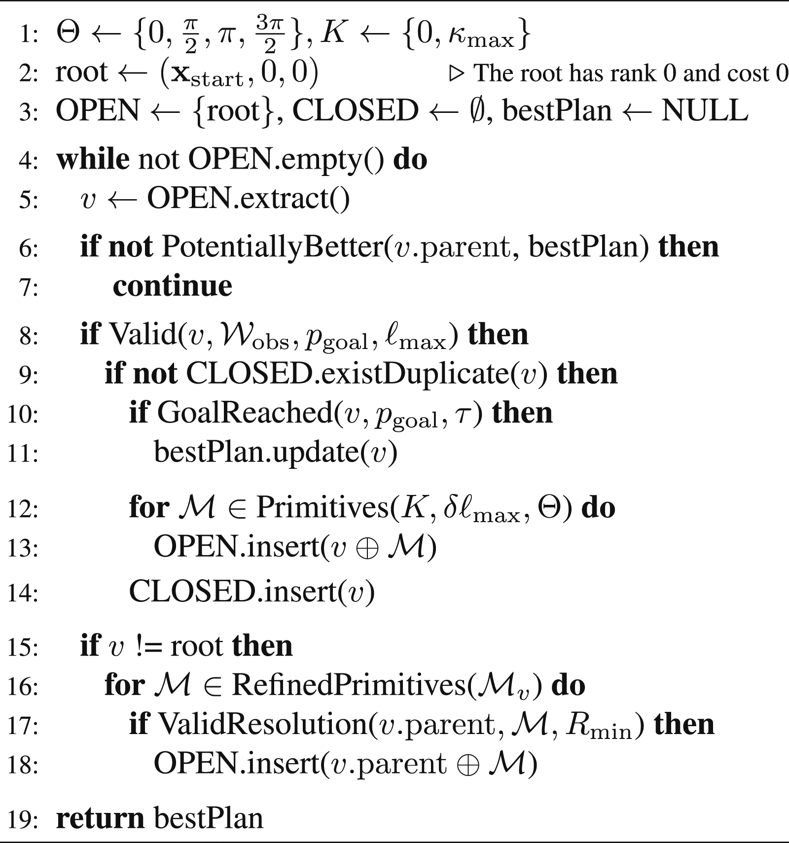
Algorithm 2 RCS*

4.1.4. Duplicate detection

To avoid re-expanding nodes with the same or highly similar configurations multiple times, search-based planners often employ duplicate detection (Du et al., 2019) that prunes so-called “duplicate” nodes. To prune duplicate nodes and enable the planner to rapidly explore the entire C-space, we reject a node if there already exists a similar configuration in the search tree (Alg. 1, line 7). More formally, we reject node v with configuration x _v if $\exists u\in \mathcal{V},\rho \left({\mathbf{x}}_u,{\mathbf{x}}_v\right)<d_{\text{sim}}$ , where d_sim > 0 is a parameter we use to identify similar configurations. Here, ρ(·) is a distance metric defined on $\mathcal{X}$ which in our work is defined as

$\rho \left({\mathbf{x}}_u,{\mathbf{x}}_v\right)={\Vert p_u-p_v\Vert }_2+\alpha \cdot {\text{dist}}_{\sphericalangle }\left(q_u,q_v\right),$

(5)

where α > 0 is a weighting parameter and dist_∢() is the angular distance between two orientations. Note that to guarantee resolution completeness, the value of d_sim depends on other system parameters detailed in Section 5.

4.2. A resolution-optimal version of RCS (RCS*)

Since RCS* can be seen as an extended version of RCS, they share many basic components, as can be seen from the pseudocode of RCS* shown in Alg. 2. In this section, we focus on explaining the differences between RCS* and RCS.

Similar to RCS, RCS* builds a search tree with motion primitives of multiple resolutions (as defined in Sections 4.1.1 and 4.1.2).

We first introduce the essential differences that guarantee the resolution optimality of RCS*.

4.2.1. Termination criteria

In RCS, the first motion plan obtained is returned directly. In a multi-resolution search, optimality of the first plan is not guaranteed. So RCS* terminates when the OPEN list is exhausted (Alg. 2, line 4), and the best plan is returned (if any is found). Resolution-Complete Search* is guaranteed to terminate in finite time due to the cutoff resolution.

4.2.2. Cost-aware duplicate detection

Similar to RCS, RCS* avoids expanding nodes with highly similar configurations by performing duplicate detection (Alg. 2, line 9). In RCS*, we additionally consider the node’s cost $\mathcal{C}\left(v\right)$ when determining whether the node is a duplicate. More specifically, a node v is determined as a duplicate if there exists a node u in the CLOSED list that satisfies (i’) ρ(x _u , x _v ) < d_sim and (ii’) $\mathcal{C}\left(u\right)\le \mathcal{C}\left(v\right)$ , where ρ is the distance function defined in Section 4.1.4. Condition (i’) is shared between RCS and RCS*, while condition (ii”) is important for keeping RCS* resolution optimal as it prevents nodes with lower cost from being pruned away by nodes with higher cost.

In Section 5, we determine the value of d_sim. Note that in RCS*, we need to specify this value correctly not only to ensure that the solution is valid but also to satisfy a desired approximation factor for trajectory cost.

4.2.3. Cost-aware node ordering

As is mentioned above, RCS* does not terminate until the search is exhausted, indicating it will, in the worst case, spend time on checking almost all possible solutions. Thus, from the perspective of computation efficiency, it is critical to find low-cost solutions early and then prune the non-promising branches in the following search. We now introduce these differences.

In each iteration of RCS*, an expansion of existing nodes is performed in an A*-like fashion. In particular, nodes are iteratively extracted from the OPEN list (Alg. 2, line 5), wherein nodes are ordered according to their rank (as defined in Section 4.1.2) and a secondary metric f(·). The secondary metric $f\left(v\right)=\mathcal{C}\left(v\right)+h\left(v\right)$ has $\mathcal{C}\left(v\right)$ denoting the cost of the trajectory from the root of $\mathcal{T}$ to v with respect to $\mathcal{C}$ and h(v) being a heuristic function estimating the cost of the trajectory from the node v to the goal point. For example, in the case where $\mathcal{C}$ is trajectory length, we have h(v) be the length of the Dubins curve (LaValle, 2006) on the plane spanned by x _v and p_goal. Unlike in RCS, where nodes with lower rank are always extracted first, RCS* relaxes this ordering by introducing a lookahead parameter denoted as $n_{\text{la}}\in \mathbb{N}$ (similar to the idea in Lindemann and LaValle (2006) and Mandalika et al. (2018)). At any time during the search, we denote the minimum rank of nodes in the OPEN list as r_open. Then we order all nodes with rank r ≤ r_open + n_la according to a secondary metric f(·). This is done to prioritize searching nodes from a coarser resolution, which speeds up finding an initial motion plan (this is similar in nature to using a focal list (Pearl and Kim, 1982) in A*-like algorithms).

4.2.4. Node pruning

In addition to the node validation conditions in RCS (Section 4.1.3), RCS* checks that the cost $\mathcal{C}\left(v\right)$ is smaller than the cost of the best plan reaching the goal region found so far. If the heuristic function h(·) is admissible, we use f(v) instead of $\mathcal{C}\left(v\right)$ for node pruning, as f(·) provides a better estimate of the node cost and hence allows to prune more nodes.

4.2.5. Open node skipping

Since f(·) is only the secondary metric for ordering nodes in the OPEN list, it is possible that a node with a higher f(·) value is processed before a node with a lower f(·). Thus, when a node is extracted from the OPEN list, we first check whether the parent node still leads to a better motion plan (Alg. 2, line 6). Denote by C* the cost of the best plan found so far. Any node v in the search tree is not promising if $\mathcal{C}\left(v\right)\ge C^{*}$ (or f(v) ≥ C* in case that h(·) is admissible). Then for a node v extracted from the OPEN list, we discard it directly if v.parent is not promising (Alg. 2, line 7).

4.3. Domain-specific optimizations

We now describe several optimizations used to further speed up the planners.

4.3.1. Early pruning by testing for goal reachability

We can prune away nodes that, due to curvature constraints, cannot be part of a path that reaches the goal (see Figure 6 for a 2D illustration). The curvature constraint defines so-called “unreachable regions” of a node and testing if the goal p_goal belongs to a node’s unreachable region can be done efficiently (see Figure 6). Such nodes are pruned away and are not expanded.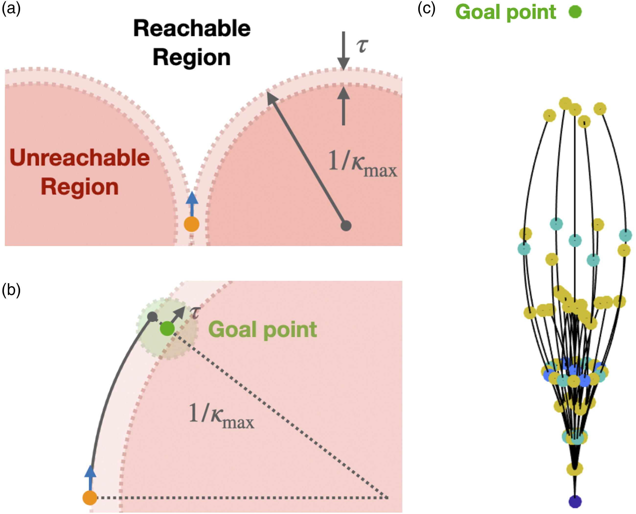

Figure 6.

(a) An illustration of reachable and unreachable regions in 2D. The case in 3D is similar. The unreachable region can be generated by rotating the circles around the Z-axis (blue vector), which creates a donut-like shape in 3D that is unreachable. It also visualizes how we check goal reachability when considering tolerance τ. We reject a configuration if the relative position of p_goal falls in the inner region (darker orange). (b) The algorithm creates a direct connection to the goal when p_goal is outside but still close to the boundary of the reachable region. We use a circular arc with curvature κ_max to steer toward p_goal and the arc stops at the closest point to p_goal. (c) An example of valid nodes with rank 0–3 after checking goal reachability.

However, recall that we allow some goal tolerance τ. Thus, instead of requiring the goal point to be inside a node’s reachable region, we only require that the distance between p_goal and the boundary of the reachable region is smaller than τ.

Note that in our setting, the needle tip cannot (physically) turn more than 90° as the needle might buckle and shear through the tissue, so we discard such motions. Thus, we do not need to account for a needle entering the unreachable region due to a “U-turn.”

4.3.2. Direct goal connection

For each node v that is added to the search tree with corresponding configuration x _v , we attempt to connect x _v to the goal point p_goal directly (a similar technique is used in the RRT-based needle planner in Patil et al. (2014)). Such a direct-connection trajectory lies in the plane determined by the tangent vector of x _v and p_goal. We consider two different types of trajectories to perform the direct connection. The first one is to use a circular arc following the idea in Patil et al. (2014). The second one is to use Dubins curve that starts with a maximum curvature arc and then follows a straight trajectory. Both types of trajectories can be deterministically computed according to the relative position of x _v and p_goal. In our implementation, circular arcs are used by default; we only use Dubins curve for RCS*, which aims to optimize the trajectory cost.

If p_goal lies outside the reachable region of x _v but the distance between p_goal and the boundary of the reachable region is no larger than τ, we steer the needle in the plane following a circular arc of curvature κ_max to the point closest to p_goal. When the circular arc is collision-free, a solution has been found and we terminate the search. This approach can often dramatically speed up the search.

4.3.3. Inevitable collision avoidance

We try to account for inevitable collisions (LaValle, 2006) to eliminate potential nodes that are bound to lead to collisions as they are expanded. In particular, for a given vertex v and the goal point, a “region-growing” process is performed from x _v within an approximation of the reachable workspace, while considering the existence of obstacles. This region is defined as the intersection of the kinematically forward-reachable workspace and the olive-shaped feasible workspace defined by x _v , p_goal, and tolerance τ (see Figure 7).

Figure 7.

A 2D illustration of the approximated reachable workspace. The kinematically forward-reachable workspace is shaded red (a 3D version can be obtained by rotating the region around the tangent vector at 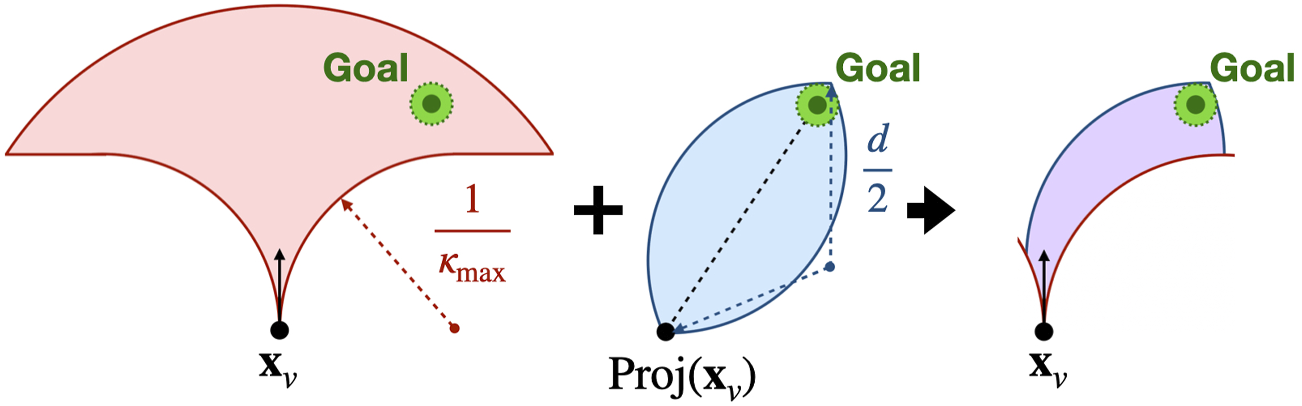x _v , which results in a trumpet shape). The feasible workspace is shaded blue. The diameter of the circular arcs is d = max(2/κ_max, τ + ‖Proj(x _v ) − p_goal‖₂). The final approximated reachable workspace is shaded in purple.

We mention that due to (i) maximum curvature constraint, (ii) maximum turning angle constraint (the needle would shear or buckle when turning over π/2), and (iii) maximum insertion length constraint, the kinematically forward-reachable workspace for a given needle configuration is a trumpet-shaped volume rooted at the current needle position (see Figure 7, left).

Additionally, a position in the workspace is potentially feasible only when there exists some orientation with which the goal region is forward reachable while the start point is backward reachable, considering the maximum curvature constraint. This defines the olive-shaped feasible workspace (see Figure 7, middle) since for any position outside the region, there is no orientation that is valid.

In the case that the goal is not reached by the grown region, v is considered to have an inevitable collision and thus to be invalid. Several examples are provided in Figure 8. Inevitable collision check allows us to efficiently identify and discard invalid branches. However, compared to previously mentioned optimizations, such inevitable collision checks can be computationally expensive and is an underestimation of the real inevitable collision. Thus, we only perform inevitable collision check when a direct goal connection fails, indicating there exist obstacles blocking the way toward the goal region. We also keep a record of states that successfully passed the inevitable collision check and skip the check when a nearby node has already passed the check, allowing us to sparsely check for inevitable collisions.

Figure 8.

2D illustration of example cases for inevitable collision check. The connected region is shaded yellow, obstacle voxels are shaded pink. This is an underestimation of inevitable collisions so even if the goal is determined as reachable in the check, it is not guaranteed that a valid motion plan to the goal exists.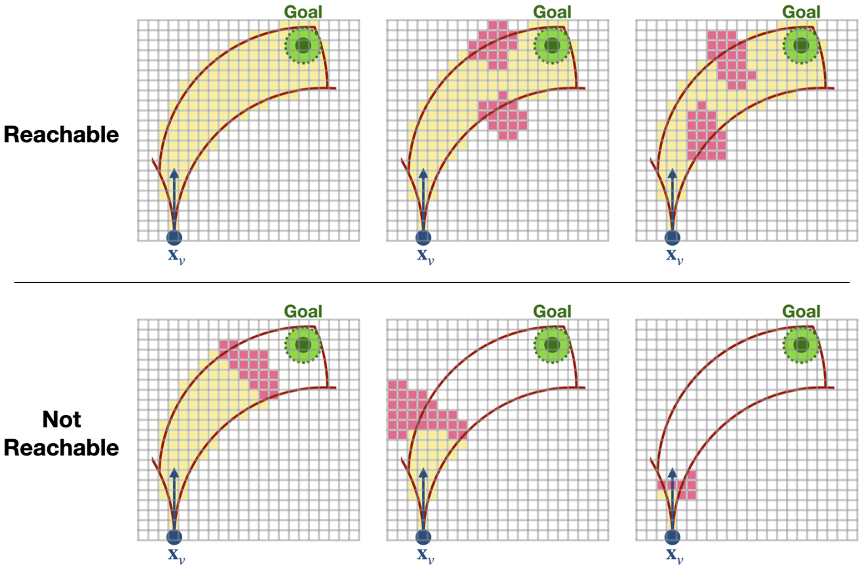

4.4. Parallelism

Our algorithms can be easily parallelized. One of the most time-consuming tasks in our search algorithm is processing a node after it is extracted from the OPEN list (namely, evaluating whether the path to this node is collision-free, and computing the relevant motion primitives for its parent node and the corresponding new nodes). To this end, we implemented a multi-threaded version of the algorithm where each thread is tasked with processing a node extracted from the OPEN list. This enables processing nodes in parallel while maintaining the correctness of the algorithm by adding standard locking mechanisms to the shared data structures (i.e., OPEN list and CLOSED set).

To distinguish between different variants of the planners, we use the notations in Table 1 in the following discussions, where “S” stands for “single-threaded,” “B” stands for “basic,” and “D” stands for “duplicates” (indicating we allow similar configurations by not doing duplicate detection).

Table 1.

Different variants of RCS and RCS*.

Name	Duplicate detection	Domain-specific optimizations	Parallelism
RCS(*)	Y	Y	Y
RCS(*)_S	Y	Y	N
RCS(*)_B	Y	N	N
RCS(*)_D	N	N	N

5. Theoretical guarantees

We study the theoretical properties of our proposed algorithms, namely, RCS and RCS*, and provide a proof for RCS and RCS* both being resolution complete while RCS* is additionally resolution optimal. We start with some general definitions pertaining to the notion of resolution completeness adapted from LaValle (2006) in Section 5.1. Unfortunately, their generality requires masking important problem-related details such as, “is planning defined in the C-space or in the control space?” or “what are the specific assumptions on the system?” This is also the reason that existing proofs (e.g., Barraquand and Latombe (1991), Appendix A) and (Cheng and LaValle, 2002, Thm. 5.2)) cannot be used as is. Thus, in Section 5.2, we quickly move to the specific setting of motion planning for steerable needles which requires specifying the exact problem-related details and definitions. We also explain in this section where we rely on the aforementioned proofs and where we are required to account for our specific domain and planner.

5.1. General resolution-related definitions

We now introduce some general definitions of resolution, resolution completeness, and resolution optimality. These general definitions will help in understanding later discussions specific to RCS and RCS*.

Definition 1

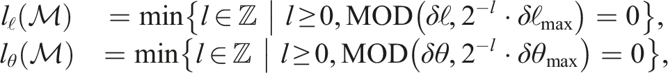
Resolution. Resolution is a finite set of parameters R = (r₀, …, r _n ), where each r _i ∈ R characterizes the discretization of some dimension in some space (e.g., state space, configuration space, action space, and time), and a smaller number indicates a finer resolution on that dimension. We say that resolution $R^1=\left(r_0^1,\dots ,r_n^1\right)$ is finer than $R^2=\left(r_0^2,\dots ,r_n^2\right)$ if $\forall i,r_i^1\le r_i^2$ and ∃j s.t. $r_j^1<r_j^2$ . ¹

Definition 2

Resolution completeness. For a general motion planning problem Δ, a planner is resolution complete if when a so-called qualified solution to Δ exists, there exists some resolution R_min such that running $\mathcal{P}$ with resolution R_min on Δ finds a solution in finite time.

Definition 3

Resolution optimality. For a general motion planning problem Δ, a planner $\mathcal{P}$ is resolution optimal if when at least one so-called qualified solution to Δ exists and the solution with optimal cost (considering a cost function $\mathcal{C}$ ) among all so-called qualified solutions is σ*, there exists some resolution R_min such that running $\mathcal{P}$ with resolution R_min on Δ finds a suboptimal solution, σ, in finite time. More specifically, $\mathcal{P}$ guarantees $\mathcal{C}\left(\sigma \right)\le \left(1+\epsilon \right)\cdot \mathcal{C}\left({\sigma }^{*}\right)$ , where ɛ is a predefined approximation parameter.

Clearly, the above definitions are more general intuitions than specific definitions for the needle-steering problem. We need to define what a “qualified solution” is and what “running $\mathcal{P}$ with resolution R_min on Δ” means.

5.2. Resolution completeness of RCS and resolution optimality of RCS*

When narrowed down to the specific case for our steerable needle planners, the notion of resolution completeness and resolution optimality can be informally stated as follows:

(i) Resolution completeness implies that RCS and RCS* are guaranteed to find a plan as long as there exists a qualified motion plan σ, assuming that the cutoff resolution R_min = (δℓ_min, δθ_min) is fine enough, both in terms of δℓ and δθ.

(ii) Resolution optimality implies that RCS* is guaranteed to find a plan whose cost is as close as desired to the cost of the globally optimal qualified motion plan σ*, assuming that the cutoff resolution R_min = (δℓ_min, δθ_min) is fine enough, both in terms of δℓ and δθ.

Thm. 1 and Thm. 2 given below state our main theoretical contribution relating to resolution completeness and resolution optimality, respectively. Before stating the main theorems, we introduce some definitions that are essential to state the assumptions in the theorems. Recall that $\mathcal{A}$ is the action space, which is the set of all valid motion primitives and that ρ(·) is a distance metric defined on $\mathcal{X}$ (equation (5)). In the following discussions, for some sequence of motion primitives M, we will use x ⊕ M to denote the resultant trajectory obtained by sequentially applying elements in M to x.

First, we provide a formal definition of Lipschitz continuity of the steerable needle system, which is used in (C1) and (C1’). We define Lipschitz continuity in our primitive-based setting, which is based on the following primitive-based metric.

Definition 4

Primitive-based metric ${\rho }_{\mathcal{A}}$ . We define a distance metric over the action space $\mathcal{A}$ as the two-way Hausdorff distance between two resultant trajectories $\mathbf{x}\oplus \left\{{\mathcal{M}}_0\right\}$ and $\mathbf{x}\oplus \left\{{\mathcal{M}}_1\right\}$ , for some configuration x and actions ${\mathcal{M}}_0,{\mathcal{M}}_1\in \mathcal{A}$ . Formally, we have

$\begin{array}{l}{\rho }_{\mathcal{A}}\left({\mathcal{M}}_0,{\mathcal{M}}_1\right)=\max \{\underset{t\in \left[0,{\ell }_1\right]}{\max }\left\{\underset{s\in \left[0,{\ell }_0\right]}{\min }\rho \left({\sigma }_0\left(s\right),{\sigma }_1\left(t\right)\right)\right\},\\ \underset{s\in \left[0,{\ell }_0\right]}{\max }\left\{\underset{t\in \left[0,{\ell }_1\right]}{\min }\rho \left({\sigma }_0\left(s\right),{\sigma }_1\left(t\right)\right)\right\}\},\end{array}$

where ${\sigma }_0=\mathbf{x}\oplus \left\{{\mathcal{M}}_0\right\}$ , ${\sigma }_1=\mathbf{x}\oplus \left\{{\mathcal{M}}_1\right\}$ , and ℓ₀, ℓ₁ are the trajectory lengths of σ₀, σ₁, respectively.

In the above definition, note that changing the initial configuration x does not change the relative position between the two trajectories. Thus, without loss of generality, we have x = (p, q) where p = (0, 0, 0) and q = (1, 0, 0, 0).

Definition 5

Lipschitz continuous. The system is Lipschitz continuous if there exists some constant L _s > 0 such that for any ${\mathbf{x}}_0,{\mathbf{x}}_1\in \mathcal{X},{\mathcal{M}}_0,{\mathcal{M}}_1\in \mathcal{A}$ , the following inequality holds:

$\rho \left({\mathbf{x}}_0\oplus {\mathcal{M}}_0,{\mathbf{x}}_1\oplus {\mathcal{M}}_1\right)\le L_s\left(\rho \left({\mathbf{x}}_0,{\mathbf{x}}_1\right)+{\rho }_{\mathcal{A}}\left({\mathcal{M}}_0,{\mathcal{M}}_1\right)\right).$

We then introduce the notions of robust and decomposable trajectories, as well as a well-behaved cost, which will be used to state the necessary conditions on the approximated motion plan σ and cost function $\mathcal{C}$ required to prove our results. The crux of the problem is that it may not be possible to approximate some plan σ using motion plans with a finite number of transitions without additional (realistic) constraints on σ and $\mathcal{C}$ .

We provide two definitions that are used to characterize motion plans that our algorithms can approximate. The first definition is concerned with trajectories that are induced by a finite set of motion primitives (not necessarily the ones used by RCS and RCS*). The second definition is concerned with so-called robust trajectories that admit some clearance from the obstacles and the boundary of the goal region. A motion plan is then considered qualified if it satisfies both definitions.

Definition 6

Decomposable trajectory. Let $\sigma :\left[0,\ell \right]\to \mathcal{X}$ be some trajectory. We say that σ is decomposable if it can be decomposed into a finite sequence of motion primitives. Namely, there exists $M_{\sigma }=\left({\mathcal{M}}_1,\dots ,{\mathcal{M}}_n\right)\subset \mathcal{A}$ , where n is finite, such that σ = σ(0) ⊕ M _σ .

Definition 7

Robust trajectory. A trajectory $\sigma :\left[0,l\right]\to \mathcal{X}$ is γ-robust, for some γ > 0, if

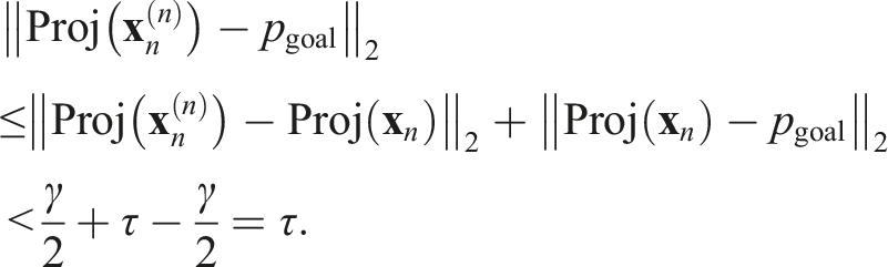
 (i) it has γ clearance from obstacles, that is, $\underset{s\in \left[0,l\right],\mathbf{x}\in {\mathcal{X}}_{\mathrm{o}\mathrm{b}\mathrm{s}}}{\min }\rho \left(\sigma \left(s\right),\mathbf{x}\right)>\gamma ,$

 (ii) its endpoint is within a distance of τ − γ to the goal point, namely, ‖Proj(σ(l)) − p_goal‖₂ < τ − γ.

Here, ${\mathcal{X}}_{\text{obs}}=\text{cl}\left(\mathcal{X}\setminus {\mathcal{X}}_{\text{free}}\right)$ and cl(·) is the closure of a set. Note that we implicitly assume here that the goal tolerance satisfies τ > γ.

We then define the notion of a well-behaved cost which states that close-by configurations have similar costs and that there are bounds on the values that the cost can attain.

Definition 8

Well-behaved cost. A configuration-based cost function c is well-behaved if

 (i) it is Lipschitz continuous, that is, $\forall {\mathbf{x}}_0,{\mathbf{x}}_1\in {\mathcal{X}}_{\text{free}}$ , |c(x₀) − c(x₁)| ≤ L _c · ρ(x₀, x₁) for some constant L _c > 0,

 (ii) $\forall \mathbf{x}\in {\mathcal{X}}_{\text{free}},c\left(\mathbf{x}\right)\in \left[c_{\min },c_{\max }\right]\subset \left(0,\infty \right)$ .

In such a case, we also say that the trajectory-based cost function $\mathcal{C}\left(\sigma \right)={\int }_0^{\ell }c\left(\sigma \left(s\right)\right)\mathrm{d}s$ is well-behaved.

We are now ready to state our main theoretical results concerning resolution completeness and resolution optimality.

Theorem 1

Resolution completeness. Let $\mathrm{\Delta }=\left(\mathcal{X},{\mathcal{W}}_{obs},{\mathbf{x}}_{start},p_{goal},\tau ,{\ell }_{\max },{\kappa }_{\max }\right)$ be a steerable needle motion planning problem. Also, suppose that the following conditions are satisfied:

(C1) The steerable needle system is Lipschitz continuous and characterized with L _s .

(C2) There exists a solution trajectory σ that is decomposable and γ-robust with γ = τ/2.

(C3) The radius d _sim used to reject similar nodes satisfies

$\begin{array}{l}{d}_{\text{sim}}<\min \left\{d_{\min },\frac{\gamma \left(L_s-1\right)}{2\left(L_s^H-1\right)}\right\},\\ where\hspace{0.17em}{d}_{\min }=\frac{2}{{\kappa }_{\max }}\sin \frac{{\kappa }_{\max }\delta {\ell }_{\min }}{2},H=\lceil \frac{{\ell }_{\max }}{\delta {\ell }_{\min }}\rceil .\end{array}$

Then RCS is resolution complete, that is, for a fine-enough cutoff resolution R_min = (δℓ_min, δθ_min), RCS will find a motion plan in finite time.

The following is a stronger property that is concerned not only with finding a solution but also with finding a “good” one.

Theorem 2

Resolution optimality. Let $\mathrm{\Delta }=\left(\mathcal{X},{\mathcal{W}}_{obs},{\mathbf{x}}_{start},p_{goal},\tau ,{\ell }_{\max },{\kappa }_{\max }\right)$ be a steerable needle motion planning problem, ${\mathrm{\Delta }}^{*}=\left(\mathrm{\Delta },\mathcal{C}\right)$ be an optimal steerable needle motion planning problem, and ɛ _cost ∈ (0, ∞) be an approximation factor. Also, suppose that the following conditions are satisfied:

(C1’) The steerable needle system is Lipschitz continuous and characterized with L _s .

(C2’)The cost function $\mathcal{C}$ is well-behaved and characterized with L _c , c_min, c_max. Denote k = (L _c + c_max)/c_min.

(C3’) The optimal solution trajectory σ* is decomposable and γ-robust with γ = min{ɛ_cost/k, τ/2}.

(C4’) The radius d _sim used to reject similar nodes satisfies

$\begin{array}{l}{d}_{\text{sim}}<\min \left\{d_{\min },\frac{\gamma \left(L_s-1\right)}{2\left(L_s^H-1\right)}\right\},\\ where\hspace{0.17em}{d}_{\min }=\frac{2}{{\kappa }_{\max }}\sin \frac{{\kappa }_{\max }\delta {\ell }_{\min }}{2},H=\lceil \frac{{\ell }_{\max }}{\delta {\ell }_{\min }}\rceil .\end{array}$

Then RCS* is resolution optimal, that is, for a fine-enough cutoff resolution R_min = (δℓ_min, δθ_min), RCS* will find a motion plan that satisfies $\mathcal{C}\left(\mathrm{\sigma }\right)\le \left(1+{\mathrm{\epsilon }}_{\mathrm{c}\mathrm{o}\mathrm{s}\mathrm{t}}\right)\cdot \mathcal{C}\left({\mathrm{\sigma }}^{*}\right)$ .

Remark 1

The above theorems can be generalized to approximate general solution trajectories that are not necessarily decomposable. In particular, since any solution trajectory has bounded curvature, it can be approximated in terms of spatial proximity and solution quality to any desired level of accuracy using a sequence of circular arcs. The latter sequence yields by definition a decomposable trajectory. Such an approximation of bounded-curvature trajectories using circular arcs (also known as biarcs) has been extensively studied in 2D (Hoschek, 1992; Meek and Walton, 1995; Sabitov and Slovesnov, 2010). Extending this argument to the 3D case is rather technical and therefore deferred to future work.

In the following sections, we provide proofs for Thm. 1 and Thm. 2. Both proofs follow two main steps. We first show that a decomposable trajectory σ can be approximated by another plan σ _ɛ that is composed solely of the motion primitives used by RCS and RCS*. Then, we show that even though RCS might not be able to exactly find σ _ɛ due to pruning, it will find another solution $\stackrel{\sim }{\sigma }$ due to the robustness of σ and the choice of d_sim, which closely follows σ _ɛ . Similarly, RCS* will be able to recover another plan ${\stackrel{\sim }{\sigma }}^{*}$ whose cost is similar to that of ${\sigma }_{\epsilon }^{*}$ (and σ*).

5.3. Approximation of decomposable trajectories

We temporarily set aside the study of our algorithms’ behavior and prove the following basic result showing that any decomposable trajectory can be approximated to any desirable degree by a finite sequence of motion primitives with fixed curvatures (discussed in Section 5.3.1) and fixed resolution (discussed in Section 5.3.2).

Before stating the theorem, we introduce notions related to trajectory approximations. We provide a formal definition of the notion of piece-wise strict ɛ-approximation. We first define this notion for a single local “piece” in the following definition, and then extend it to trajectories consisting of several pieces.

Definition 9

Local strict approximation. For two trajectories $\sigma :\left[0,\ell \right]\to \mathcal{X}$ and $\stackrel{\sim }{\sigma }:\left[0,\stackrel{\sim }{\ell }\right]\to \mathcal{X}$ , and a value ɛ > 0, we say $\stackrel{\sim }{\sigma }$ is a local strict ɛ-approximation of σ if

(i) $\stackrel{\sim }{\ell }\le \left(1+\epsilon \right)\cdot \ell$ ,

(ii) $\forall s\in [0,\min \left(\ell ,\stackrel{\sim }{\ell }\right)),\rho \left(\sigma \left(s\right),\stackrel{\sim }{\sigma }\left(s\right)\right)\le \mathrm{\epsilon }$ ,

(iii) $\forall s\in \left[\min \left(\ell ,\stackrel{\sim }{\ell }\right),\stackrel{\sim }{\ell }\right],\rho \left(\sigma \left(\ell \right),\stackrel{\sim }{\sigma }\left(s\right)\right)\le \epsilon$ .

Definition 10

Piece-wise strict approximation. For two trajectories $\sigma :\left[0,\ell \right]\to \mathcal{X}$ and $\stackrel{\sim }{\sigma }:\left[0,\stackrel{\sim }{\ell }\right]\to \mathcal{X}$ , and a value ɛ > 0, we say $\stackrel{\sim }{\sigma }$ is a piece-wise strict ɛ-approximation of σ if there exist two sequences s₀ < s₁ < … < s _n and ${\stackrel{\sim }{s}}_0<{\stackrel{\sim }{s}}_1<\dots <{\stackrel{\sim }{s}}_n$ such that

(i) $s_0=0,{\stackrel{\sim }{s}}_0=0$ ,

(ii) $s_n=\ell ,{\stackrel{\sim }{s}}_n=\stackrel{\sim }{\ell }$ ,

(iii) ∀i ∈ [0, n − 1], the sub-trajectory $\stackrel{\sim }{\sigma }\left({\stackrel{\sim }{s}}_i,{\stackrel{\sim }{s}}_{i+1}\right)$ is a local strict ɛ-approximation of σ(s _i , s_i+1).

Additionally, it will be convenient to introduce the notion of a finest set of motion primitives.

Definition 11

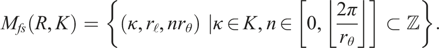
Finest set of motion primitives. Given a resolution R = (r _ℓ , r _θ ), and a set of curvatures K, we define the finest set of motion primitives as

$M_{fs}\left(R,K\right)=\left\{\left(\kappa ,r_{\ell },n{r}_{\theta }\right) |\kappa \in K,n\in \left[0,\lfloor \frac{2\pi }{r_{\theta }}\rfloor \right]\subset \mathbb{Z}\right\}.$

We now state the following theorem about trajectory approximation.

Theorem 3

Let σ be a decomposable trajectory and let ɛ > 0 be some real value. If the system is Lipschitz continuous, there exists a fine resolution R(σ, ɛ) = (r _ℓ , r _θ ) and a finite sequence of motion primitives M_R(σ,ɛ) ⊆ M _fs (R(σ, ɛ), {0, κ_max}) such that σ _ɛ ≔σ(0) ⊕ M_R(σ,ɛ) is a piece-wise strict ɛ-approximation of σ. Moreover, when we also consider a cost function, if c is a well-behaved cost (characterized with L _c , c_min, c_max), then the trajectory cost satisfies $\mathcal{C}\left({\sigma }_{\epsilon }\right)\le \left(1+k\cdot \epsilon \right)\cdot \mathcal{C}\left(\sigma \right)$ , where k = (L _c + c_max)/c_min.

We break the proof of this result into the following steps. In the following discussions, we refer to the parameters of $\mathcal{M}=\left(\kappa ,\delta \ell ,\delta \theta \right)$ as $\mathcal{M}.\kappa$ , $\mathcal{M}.\delta \ell$ , and $\mathcal{M}.\delta \theta$ , respectively.

5.3.1. Approximating arbitrary curvatures using duty-cycling

As a first step, we show that any decomposable trajectory σ can be approximated arbitrarily well by a finite sequence of motion primitives whose curvature is either 0 or κ_max. We provide a justification of this property below.

When a bevel-tip needle is inserted without rotations, it follows a trajectory with curvature κ_max. When the needle is inserted while applying axial rotational velocity that is relatively larger than the insertion velocity, it follows a straight line (i.e., of curvature zero). Minhas et al. (2007) introduced the notion of duty-cycling to approximate any curvature for bevel-tip steerable needles. Roughly speaking, combining periods of needle spinning (i.e., zero-curvature trajectories) with periods of non-spinning (i.e., maximal-curvature trajectories) enables the needle to achieve any curvature up to the maximum needle curvature. This idea is formalized in the following lemma.

Lemma 1

Approximating arbitrary curvatures using duty-cycling. Let σ be a decomposable trajectory and let ɛ _d > 0 be some real value. There exists a finite sequence of motion primitives M _D in which every element has curvature κ ∈ {0, κ_max} such that the trajectory σ(0) ⊕ M _D is a piece-wise strict ɛ _d -approximation of σ.

Proof. Here, to explicitly show how the approximation factor ɛ _d is used and to provide a more general discussion, we provide a proof from a geometric perspective (and not control-based as in the original work in Minhas et al. (2007)).

As the trajectory σ is decomposable, there exists a sequence of motion primitives 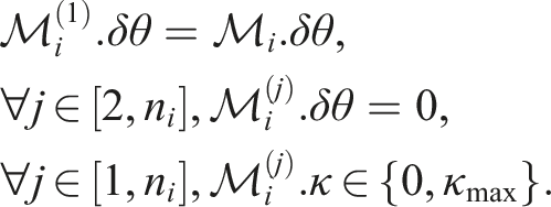$M_{\sigma }=\left\{{\mathcal{M}}_1,\dots ,{\mathcal{M}}_n\right\}$ such that σ = σ(0) ⊕ M _σ and each motion primitive ${\mathcal{M}}_i$ has arbitrary curvature κ _i ∈ [0, κ_max]. To approximate ${\mathcal{M}}_i$ , we construct a sequence of motion primitives $M_i=\left\{{\mathcal{M}}_i^{\left(1\right)},\dots ,{\mathcal{M}}_i^{\left(n_i\right)}\right\}$ that satisfies

$\begin{array}{l}{\mathcal{M}}_i^{\left(1\right)}.\delta \theta ={\mathcal{M}}_i.\delta \theta ,\\ \forall j\in \left[2,n_i\right],{\mathcal{M}}_i^{\left(j\right)}.\delta \theta =0,\\ \forall j\in \left[1,n_i\right],{\mathcal{M}}_i^{\left(j\right)}.\kappa \in \left\{0,{\kappa }_{\max }\right\}.\end{array}$

Namely, the first motion primitive ${\mathcal{M}}_i^{\left(1\right)}$ ensures that both trajectories use the same curving plane and the rest of the sequence stays within this curving plane and approximates the (arbitrary) curvature κ _i .

We then decompose ${\mathcal{M}}_i$ into small equal-length segments of length ℓ _i where the specific value of ℓ _i is chosen according to the value of ɛ _d and ${\mathcal{M}}_i$ ’s curvature κ _i . We then use three motion primitives to approximate each of these segments as illustrated in Figure 9. Denote the j-th segment along ${\mathcal{M}}_i$ as ${\mathcal{M}}_{ij}$ and the corresponding sequence of three primitives approximating ${\mathcal{M}}_{ij}$ as $M_{ij}=\left\{{\mathcal{M}}_{ij}^0,{\mathcal{M}}_{ij}^1,{\mathcal{M}}_{ij}^2\right\}$ . Note that (i) the start and end configurations of ${\mathcal{M}}_{ij}$ and M _ij are identical, (ii) the two-way Hausdorff distance between ${\mathcal{M}}_{ij}$ and M _ij is less than ɛ _i if ℓ _i is carefully chosen, and (iii) for each segment with length ℓ _i , the length of the three-segment approximation is less than (1 + ɛ _i ) · ℓ _i if ℓ _i is carefully chosen. The point-wise distance is then bounded by ɛ _i (1 + ℓ _i ) + ακℓ _i /2 (recall that α is the weighting parameter in the distance metric equation (5)). See Figure 9 for details. Thus, by carefully choosing ɛ _i , we can make sure the three-segment approximation M _ij is a local strict ɛ _d -approximation of the original segment ${\mathcal{M}}_{ij}$ , where ɛ _i (1 + ℓ _i ) + ακℓ _i /2 ≤ ɛ _d .

Figure 9.

Illustration of approximating arbitrary curvatures using duty-cycling. 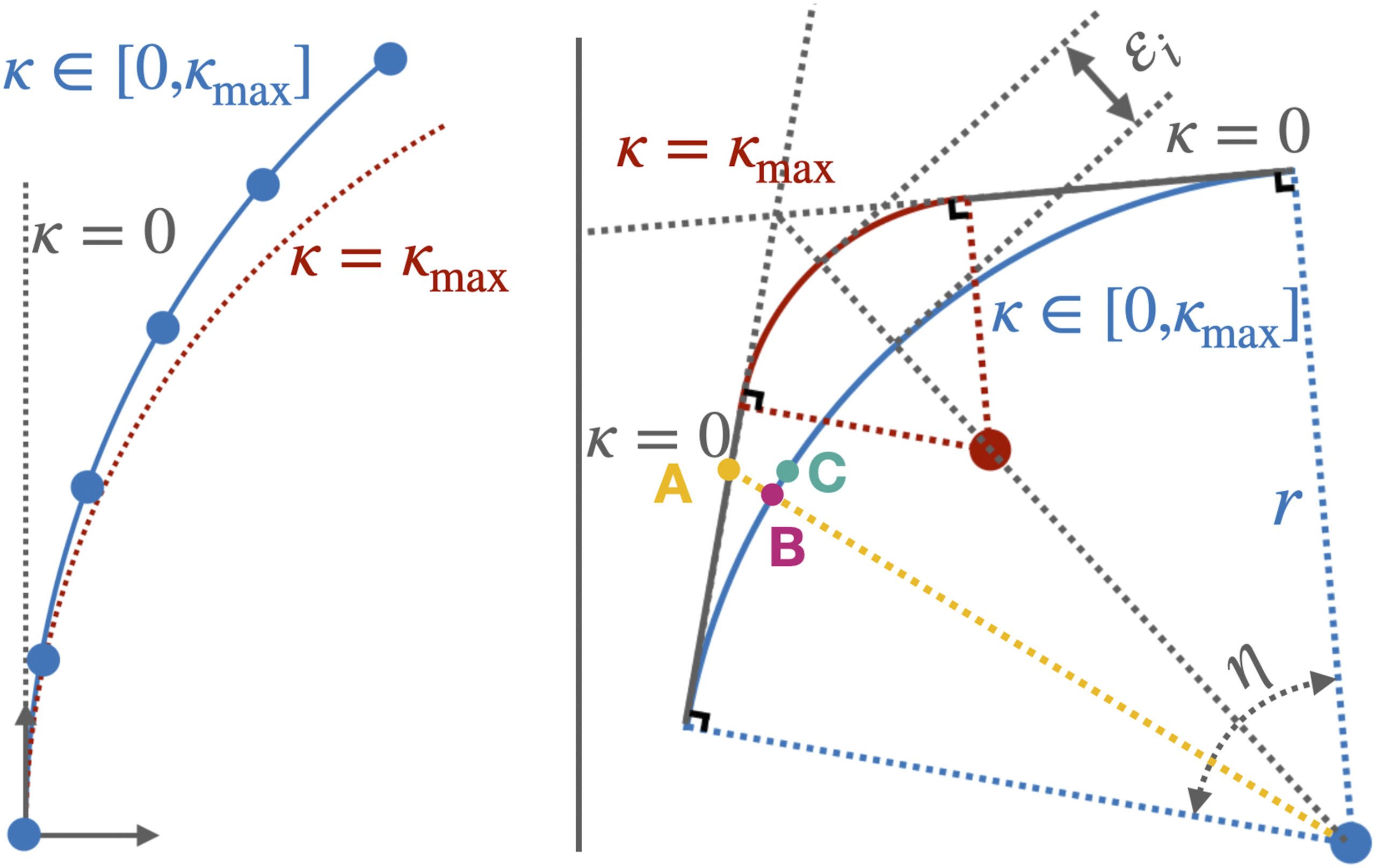Left: Decompose ${\mathcal{M}}_i$ into multiple segments with length ℓ _i . Right: Use three segments to approximate one segment of ${\mathcal{M}}_i$ , where the segments have a curvature of 0, κ_max and 0, respectively. The two-way Hausdorff distance (the positional part marked as ɛ _i in the figure) depends on ℓ _i . For a given κ_max, to approximate ${\mathcal{M}}_i$ (with curvature κ), the shorter ℓ _i is, the smaller ɛ _i is. This is because ɛ _i < r · (1/cos(0.5η) − 1), where r = 1/κ is the radius of curvature and η = ℓ _i /r is the central angle. Since the maximum orientation difference along the trajectory is bounded by 0.5η, the two-way Hausdorff distance in configuration space is also bounded. Also, the trajectory length of the original segment is ℓ _i = r · η, and the length of the three-segment trajectory is ℓ_approx ≤ 2r · tan(0.5η). Since lim_η→02 tan(0.5η)/η = 1, the trajectory length ratio approaches 1 when η approaches 0. This means the trajectory length can be approximated arbitrarily well. Furthermore, the point-wise distance is bounded by ɛ _i (1 + ℓ _i ) + αℓ _i /(2r), when we have a small enough ℓ _i that ℓ_approx ≤ (1 + ɛ _i )ℓ _i . As is shown in the figure, A and B are points intersecting with a straight line originating from the center of curvature, and C is A’s corresponding point along ${\mathcal{M}}_i$ . Then ‖A − B‖ ≤ ɛ _i and the length of curve BC ≤ ɛ _i ℓ _i , and thus ‖A − C‖ ≤ ɛ _i (1 + ℓ _i ). Additionally, the orientation difference between A and C is bounded by 0.5η = ℓ _i /(2r).

Let $M_{\sigma }^{{\epsilon }_d}=M_1\cdot M_2\cdot \dots \cdot M_n$ be this sequence of all the newly constructed motion primitives. By definition, $\sigma \left(0\right)\oplus M_{\sigma }^{{\epsilon }_d}$ is a piece-wise strict ɛ _d -approximation of σ.□

5.3.2. Approximating curves using fixed-resolution primitives

After the previous step, a decomposable trajectory can be approximated by another decomposable trajectory with only 0 or κ_max curvature, although the approximation might require different resolutions. Next, we further show that a decomposable trajectory can be approximated by fixed-resolution primitives.

Lemma 2

Approximating curves using fixed-resolution primitives. Let σ be a decomposable trajectory and let ɛ _r > 0 be some real value. If the system is Lipschitz continuous (Def. 5), there exists a fine resolution R(σ, ɛ _r ) = (r _ℓ , r _θ ) and a finite sequence of motion primitives $M_{R\left(\sigma ,{\epsilon }_r\right)}$ such that $\sigma \left(0\right)\oplus M_{R\left(\sigma ,{\epsilon }_r\right)}$ is a piece-wise strict ɛ _r -approximation of σ. Moreover, $M_{R\left(\sigma ,{\epsilon }_r\right)}\subseteq {\mathcal{M}}_{\text{fs}}\left(R\left(\sigma ,{\epsilon }_r\right),K_{\sigma }\right)$ , where K _σ is the set of curvatures that appear along σ.

Proof. ² The trajectory σ is decomposable; thus, there exists a finite sequence of motion primitives $M_{\sigma }=\left\{{\mathcal{M}}_1,\dots ,{\mathcal{M}}_n\right\}$ such that σ = σ(0) ⊕ M _σ . Set $K_{\sigma }=\underset{i}{\cup }{\mathcal{M}}_i.\kappa$ to be the set of all curvatures that appear in M _σ .

To approximate each motion primitive 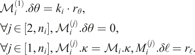${\mathcal{M}}_i$ using primitives from the finest set of motion primitives ${\mathcal{M}}_{\text{fs}}\left(R\left(\sigma ,{\epsilon }_r\right),K_{\sigma }\right)$ (Def. 11), we construct a sequence motion primitive $M_i=\left\{{\mathcal{M}}_i^{\left(1\right)},\dots {\mathcal{M}}_i^{\left(n_i\right)}\right\}$ , where

$\begin{array}{l}{\mathcal{M}}_i^{\left(1\right)}.\delta \theta =k_i\cdot r_{\theta },\\ \forall j\in \left[2,n_i\right],{\mathcal{M}}_i^{\left(j\right)}.\delta \theta =0,\\ \forall j\in \left[1,n_i\right],{\mathcal{M}}_i^{\left(j\right)}.\kappa ={\mathcal{M}}_i.\kappa ,M_i^{\left(j\right)}.\delta \ell =r_{\ell }.\end{array}$

Here, the first motion primitive ${\mathcal{M}}_i^{\left(1\right)}$ accounts for the curving plane (though here it can only be approximated) and the rest of the sequence stays within this curving plane and accounts for the length of the circular arc the trajectory follows in this plane. Applying the sequence M _i is equivalent to applying one motion primitive ${\stackrel{\sim }{\mathcal{M}}}_i=\left({\mathcal{M}}_i.\kappa ,n_i\cdot r_{\ell },k_i\cdot r_{\theta }\right)$ . Thus, by carefully choosing r _ℓ and r _θ , the distance between ${\mathcal{M}}_i$ and ${\stackrel{\sim }{\mathcal{M}}}_i$ (see Def. 4) can be arbitrarily small.

This is done for every motion primitive 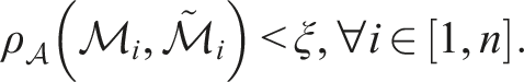${\mathcal{M}}_i$ . As M _σ is a finite sequence of size n, for any ξ > 0, we can always find a fine-enough resolution (r _ℓ , r _θ ) that ensures that

${\rho }_{\mathcal{A}}\left({\mathcal{M}}_i,{\stackrel{\sim }{\mathcal{M}}}_i\right)<\xi ,\forall i\in \left[1,n\right].$

This is because given that both motion primitives have equal curvature, ${\rho }_{\mathcal{A}}\left({\mathcal{M}}_1,{\mathcal{M}}_2\right)<\left|\delta {\theta }_1-\delta {\theta }_2\right|\cdot \min \left\{\delta {\ell }_1,\delta {\ell }_2\right\}+\left|\delta {\ell }_1-\delta {\ell }_2\right|+\alpha \left(\left|\delta {\theta }_1-\delta {\theta }_2\right|+\left|\delta {\ell }_1-\delta {\ell }_2\right|/{\mathcal{M}}_i.\kappa \right)$ , where $\delta {\ell }_i={\mathcal{M}}_i.\delta \ell$ and $\delta {\theta }_i={\mathcal{M}}_i.\delta \theta$ . The above upper bound for the action-space distance accounts for both position and orientation. See Figure 10 for illustration.

Figure 10.

Illustration of the action distance between two motion primitives with the same curvature. Here, the shorter motion primitive lies in curving plane 1; thus, min{δℓ₁, δℓ₂} = OA_curv and |δℓ₁ − δℓ₂| = OC_curv − OA_curv = BC_curv. Meanwhile, the orientation difference between A and C satisfies dist_∢(A, C) ≤ dist_∢(A, B) + dist_∢(B, C).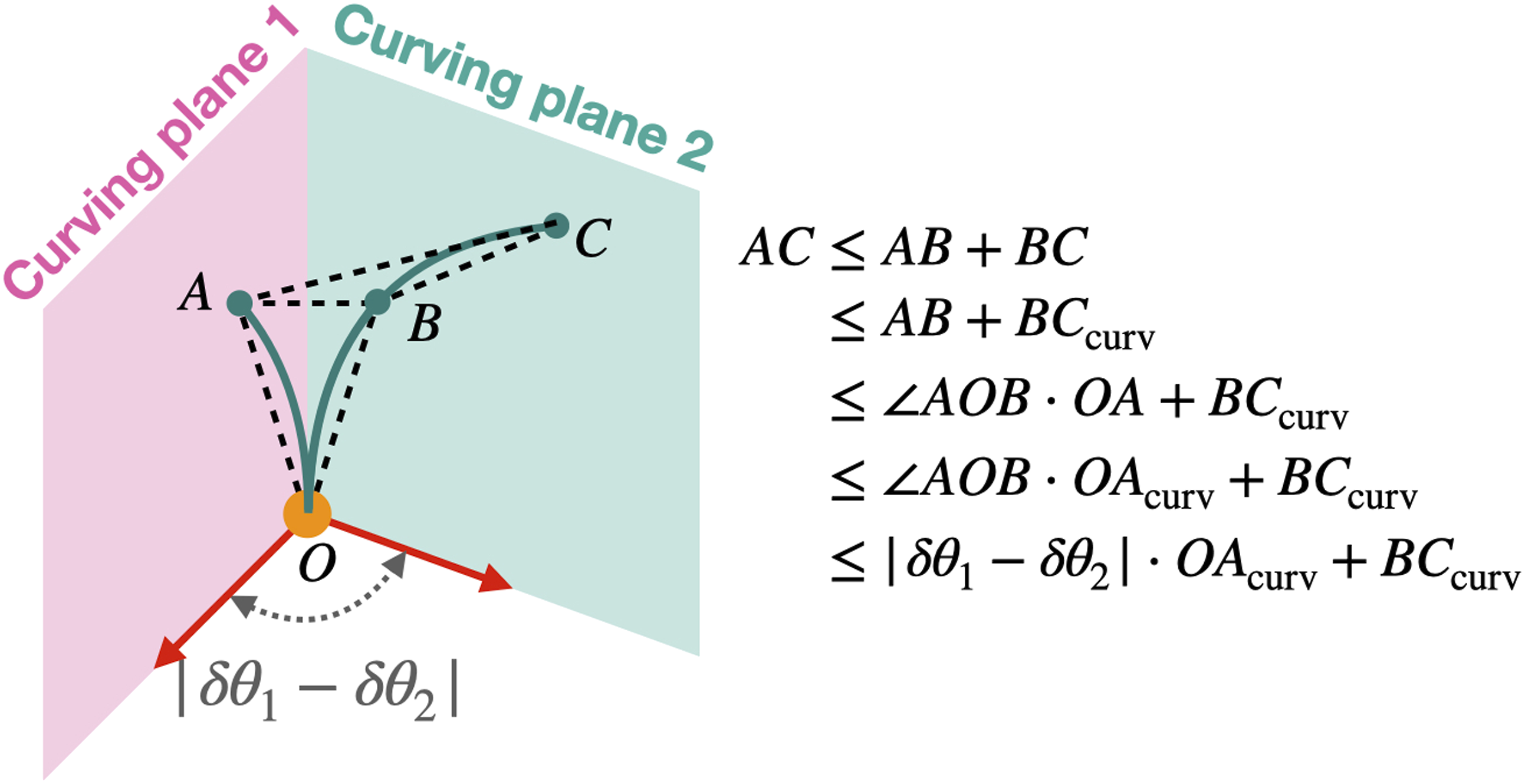

Since the system is Lipschitz continuous,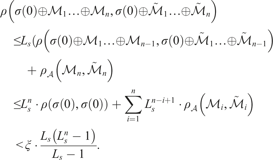

$\begin{array}{l}\rho \left(\sigma \left(0\right)\oplus {\mathcal{M}}_1\dots \oplus {\mathcal{M}}_n,\sigma \left(0\right)\oplus {\stackrel{\sim }{\mathcal{M}}}_1\dots \oplus {\stackrel{\sim }{\mathcal{M}}}_n\right)\\ \le L_s(\rho (\sigma \left(0\right)\oplus {\mathcal{M}}_1\dots \oplus {\mathcal{M}}_{n-1},\sigma \left(0\right)\oplus {\stackrel{\sim }{\mathcal{M}}}_1\dots \oplus {\stackrel{\sim }{\mathcal{M}}}_{n-1})\\ +{\rho }_{\mathcal{A}}\left({\mathcal{M}}_n,{\stackrel{\sim }{\mathcal{M}}}_n\right)\\ \le L_s^n\cdot \rho \left(\sigma \left(0\right),\sigma \left(0\right)\right)+{\displaystyle \sum }_{i=1}^n{L}_s^{n-i+1}\cdot {\rho }_{\mathcal{A}}\left({\mathcal{M}}_i,{\stackrel{\sim }{\mathcal{M}}}_i\right)\\ <\xi \cdot \frac{L_s\left(L_s^n-1\right)}{L_s-1}.\end{array}$

Thus, to ensure that $\sigma \left(0\right)\oplus \left\{{\stackrel{\sim }{\mathcal{M}}}_1,\dots ,{\stackrel{\sim }{\mathcal{M}}}_n\right\}$ is a piece-wise strict ɛ _r -approximation of σ, we only need to ensure that $\xi \le {\epsilon }_r\left(L_s-1\right)/{\mathrm{(L}}_s\left(L_s^n-1\right)$ ). As both n and L _s are fixed, we can choose ξ to be as small as needed. Thus, the desired fine resolution exists which concludes the proof.□

Having established Lem. 2, we can finalize the first part of Thm. 3. Namely, we carefully set ɛ _d and ɛ _r , so that the final result is a piece-wise strict ɛ-approximation.

Set ${\epsilon }_d={\epsilon }_r=\sqrt{1+\epsilon }-1$ . According to Lem. 1, there exists a finite sequence of motion primitives M _D in which every element has curvature κ ∈ {0, κ_max} such that the trajectory σ _d = σ(0) ⊕ M _D is a piece-wise strict ɛ _d -approximation of σ.

Note that by construction σ _d is decomposable. Thus, according to Lem. 2, there exists a fine resolution R(σ, ɛ _r ) = (r _ℓ , r _θ ) and a finite sequence of motion primitives $M_{R\left(\sigma ,{\epsilon }_r\right)}$ such that ${\sigma }_r=\sigma \left(0\right)\oplus M_{R\left(\sigma ,{\epsilon }_r\right)}$ is a piece-wise strict ɛ _r -approximation of σ _d . Moreover, $M_{R\left(\sigma ,{\epsilon }_r\right)}\subseteq {\mathcal{M}}_{\text{fs}}\left(R\left(\sigma ,{\epsilon }_r\right),\left\{0,{\kappa }_{\max }\right\}\right)$ as the construction in the proof of Lem. 2 does not add new curvatures.

Finally, as ${\epsilon }_d={\epsilon }_r=\sqrt{1+\epsilon }-1$ , the trajectory σ _r is a piece-wise strict ɛ-approximation of σ. This is because for every step above, we use segments of shorter lengths for the approximation; thus, segments along σ _r and σ satisfy conditions (ii) and (iii) in Def. 9 with a distance upper bound of (ɛ _d + ɛ _r ). So we only need to take care of the first condition in Def. 9. Having ${\epsilon }_d={\epsilon }_r=\sqrt{1+\epsilon }-1$ would provide us with (1 + ɛ _d )(1 + ɛ _r ) = 1 + ɛ; thus, the trajectory length is also bounded, making segments in σ _r local strict ɛ-approximations of the corresponding segments in σ. By definition, σ _r is a piece-wise strict ɛ-approximation of σ.

5.3.3. Similar cost for piece-wise strict approximations

To finish the proof of Thm. 3, we finally show that the approximation of σ also achieves a desirable cost.

Lemma 3

Similar cost for local strict approximations. If a trajectory $\stackrel{\sim }{\sigma }$ is a local strict ɛ-approximation of another trajectory σ, and the cost function $\mathcal{C}$ is well-behaved (characterized with L _c , c_min, c_max), then we have $\mathcal{C}\left(\stackrel{\sim }{\sigma }\right)\le \left(1+k\cdot \epsilon \right)\cdot \mathcal{C}\left(\sigma \right)$ , where k = (L _c + c_max)/c_min.

Proof. We have

$\begin{array}{l}\mathcal{C}\left(\stackrel{\sim }{\sigma }\right)={\int }_0^{l^{\prime }}c\left(\stackrel{\sim }{\sigma }\left(s\right)\right)ds\\ ={\int }_0^{l}c\left(\stackrel{\sim }{\sigma }\left(s\right)\right)ds+{\int }_l^{l^{\prime }}c\left(\stackrel{\sim }{\sigma }\left(s\right)\right)ds\\ \le {\int }_0^l\left(c\left(\sigma \left(s\right)\right)+L_c\cdot \epsilon \right)\hspace{0.17em}ds+\epsilon \cdot l\cdot c_{\max }\\ ={\int }_0^l\left(c\left(\sigma \left(s\right)\right)+L_c\cdot \epsilon +c_{\max }\cdot \epsilon \right)\hspace{0.17em}ds\\ ={\int }_0^l\left(1+\frac{\epsilon \left(L_c+c_{\max }\right)}{c\left(\sigma \left(s\right)\right)}\right)\cdot c\left(\sigma \left(s\right)\right)ds\\ \le {\int }_0^l\left(1+\frac{\epsilon \left(L_c+c_{\max }\right)}{c_{\min }}\right)\cdot c\left(\sigma \left(s\right)\right)ds\\ =\left(1+\frac{\epsilon \left(L_c+c_{\max }\right)}{c_{\min }}\right)\cdot {\int }_0^{l}c\left(\sigma \left(s\right)\right)ds\\ =\left(1+\frac{\epsilon \left(L_c+c_{\max }\right)}{c_{\min }}\right)\cdot \mathcal{C}\left(\sigma \right).\square \end{array}$

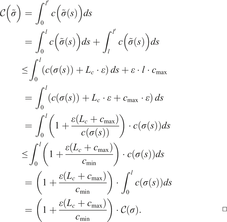
To conclude, if every piece of the sub-trajectory is bounded, the sum of costs of all pieces is then also bounded. Thus, if a trajectory $\stackrel{\sim }{\sigma }$ is a piece-wise strict ɛ-approximation of σ, then for a well-behaved cost, we also have $\mathcal{C}\left(\stackrel{\sim }{\sigma }\right)\le \left(1+k\cdot \epsilon \right)\cdot \mathcal{C}\left(\sigma \right)$ .

5.4. Proof of Thm. 1 and Thm. 2

We are in a position to complete the proof of Thm. 1 and Thm. 2. Since the proof for Thm. 2 follows a similar idea as the proof for Thm. 1, we first prove Thm. 1 and then add the essential part that is unique to Thm. 2.

To prove Thm. 1, we first consider a simplified version of RCS, termed RCS_D, which does not use node pruning as part of duplicate detection (Alg. 1, line 7) and later extend it to RCS. For simplicity, we assume that both RCS_D and RCS do not use the additional optimizations described in Section 4.3 or ,4.4 which do not affect the validity of arguments used below.

5.4.1. Resolution completeness of RCS_D

We show that Thm. 1 holds for RCS_D. Since duplicate detection is not applied, (C3) is not considered.

Let σ be a valid solution to problem Δ that is decomposable and γ-robust. Following Thm. 3, there exists a fine resolution R(σ, ɛ) = (r _ℓ , r _θ ) and a finite sequence of motion primitives M_R(σ,ɛ) ⊆ M_fs(R(σ, ɛ), {0, κ_max}) such that σ(0) ⊕ M_R(σ,ɛ) is a piece-wise strict ɛ-approximation of σ. In our algorithm, the resolutions are divided by half as the length level l _ℓ and angle level l _θ increase. Thus, there exists a fine-enough resolution $\stackrel{\sim }{R}=\left(2^{-l_{\ell }}\cdot \delta {\ell }_{\max },2^{-l_{\theta }}\cdot \delta {\theta }_{\max }\right)$ that satisfies $2^{-k_{\ell }}\cdot \delta {\ell }_{\max }<r_{\ell }$ , $2^{-k_{\theta }}\cdot \delta {\theta }_{\max }<r_{\theta }$ . Setting the cutoff resolution R_min to be finer (both with respect to the insertion as well as rotation) than $\stackrel{\sim }{R}$ ensures that M_R(σ,ɛ) can be approximated arbitrarily well. ³

The search tree built with RCS_D is a subtree of a dense tree in which each node is expanded with every element in ${\mathcal{M}}_{\text{fs}}\left(\stackrel{\sim }{R},\left\{0,{\kappa }_{\max }\right\}\right)$ . This is because every coarse motion primitive used in RCS_D can be decomposed into a sequence of motion primitives in ${\mathcal{M}}_{\text{fs}}\left(\stackrel{\sim }{R},\left\{0,{\kappa }_{\max }\right\}\right)$ . Since the dense tree encodes all possible trajectories that can be decomposed with ${\mathcal{M}}_{\text{fs}}\left(\stackrel{\sim }{R},\left\{0,{\kappa }_{\max }\right\}\right)$ , a piece-wise strict ɛ-approximation of σ, denoted as σ _ɛ , will be encoded in the dense tree.

Next, we take ɛ = γ/2 and show that σ _ɛ is collision-free and satisfies the desired goal tolerance, which implies that RCS_D will be able to find it. According to condition (C2), σ is γ-robust. This implies that σ _ɛ is at least (γ − ɛ)-robust. Given that ɛ = γ/2, we further have σ _ɛ is γ/2-robust. Thus, for a cutoff resolution R_min that is fine enough, σ _ɛ will be explored by the search tree constructed by RCS_D.

5.4.2. Accounting for pruning in RCS

Since RCS_D terminates in finite time, RCS also terminates in finite time since more nodes are rejected. We now prove that RCS can find a solution plan if conditions (C1)-(C3) in Thm. 1 are satisfied. ⁴

Since $\sigma :\left[0,\ell \right]\to \mathcal{X}$ is a valid solution, there exists some fine resolution R(σ, ɛ) that can be used by RCS as the cutoff resolution (as discussed above), with which we can construct a piece-wise strict ɛ-approximation of σ. Denote the decomposable approximation as σ _ɛ , and the sequence of motion primitives to compose it as $M_{{\sigma }_{\epsilon }}=\left\{{\mathcal{M}}_1,\dots ,{\mathcal{M}}_n\right\}$ . When $M_{{\sigma }_{\epsilon }}$ is sequentially applied to x_start, we obtain a sequence of configurations {x₀, x₁, …, x _n }, where ${\mathbf{x}}_0={\mathbf{x}}_{\text{start}},{\mathbf{x}}_i={\mathbf{x}}_{i-1}\oplus {\mathcal{M}}_i,i\in \left[1,n\right]$ . For the rest of the proof, we use $M_{{\sigma }_{\epsilon }}\left[i,j\right]=\left\{{\mathcal{M}}_i,\dots ,{\mathcal{M}}_j\right\}$ to denote a subsequence of $M_{{\sigma }_{\epsilon }}$ . We also use $\mathbf{x}+M_{{\sigma }_{\epsilon }}\left[i,j\right]$ to denote the configuration after sequentially applying $\left\{{\mathcal{M}}_i,\dots ,{\mathcal{M}}_j\right\}$ to x.

If we run RCS_D, every x _i will be explored and σ _ɛ will be constructed when the search terminates. However, if we run RCS, we prune nodes using duplicate detection (Section 4.1.4). Thus, we need to show that even with pruning, RCS will still find a plan. This will be done by showing that the same sequence of motion primitives can be applied to configurations that are “similar” to x₀…x _n and the resultant plan $\stackrel{\sim }{\sigma }$ exists using the fact that $\stackrel{\sim }{\sigma }$ is “similar” to σ _ɛ (thus “similar” to σ) and that σ is γ-robust. The rest of this proof formalizes this idea.

Recall that (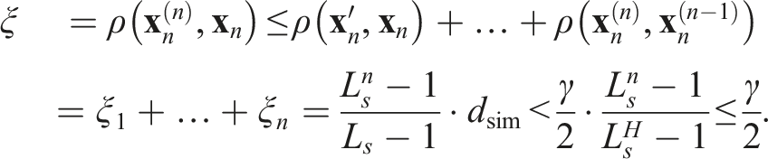C3) defines d_min, which is the minimum positional difference between a node and its successor. The condition d_sim < d_min in (C3) guarantees that any successor node is not pruned by its parent node, which keeps the tree expanding. Now, let x _i be the first configuration that is pruned because of a similar configuration (see Alg. 1, line 7). We will say that x _i is replaced by a similar configuration ${\mathbf{x}}_i^{\prime }$ . As i ≥ 1, in the worst case, we have i = 1. We then apply $M_{{\sigma }_{\epsilon }}\left[2,n\right]$ to ${\mathbf{x}}_1^{\prime }$ . According to (C1), the maximal error accumulated to ${\mathbf{x}}_n^{\prime }={\mathbf{x}}_1^{\prime }+M_{{\sigma }_{\epsilon }}\left[2,n\right]$ is ${\xi }_1=\rho \left({\mathbf{x}}_n^{\prime },{\mathbf{x}}_n\right)=L_s^{n-1}\cdot d_{\text{sim}}$ . Similarly, when ${\mathbf{x}}_2^{\prime }$ is replaced by ${\mathbf{x}}_2^{″}$ , we apply $M_{{\sigma }_{\epsilon }}\left[3,n\right]$ to ${\mathbf{x}}_2^{″}$ and for ${\mathbf{x}}_n^{″}={\mathbf{x}}_2^{″}+M_{{\sigma }_{\epsilon }}\left[3,n\right]$ , the accumulated error is ${\xi }_2=\rho \left({\mathbf{x}}_n^{″},{\mathbf{x}}_n^{\prime }\right)=L_s^{n-2}\cdot d_{\text{res}}$ . The same analysis applies for {x₃, …, x _n }. According to (C3), the total accumulated error then becomes:

$\begin{array}{cc}\xi & =\rho \left({\mathbf{x}}_n^{\left(n\right)},{\mathbf{x}}_n\right)\le \rho \left({\mathbf{x}}_n^{\prime },{\mathbf{x}}_n\right)+\dots +\rho \left({\mathbf{x}}_n^{\left(n\right)},{\mathbf{x}}_n^{\left(n-1\right)}\right)\\ & ={\xi }_1+\dots +{\xi }_n=\frac{L_s^n-1}{L_s-1}\cdot d_{\text{sim}}<\frac{\gamma }{2}\cdot \frac{L_s^n-1}{L_s^H-1}\le \frac{\gamma }{2}.\end{array}$

Next, we show that even in the worst case, the final state of $\stackrel{\sim }{\sigma }$ (i.e., ${\mathbf{x}}_n^{\left(n\right)}$ ) satisfies goal tolerance τ. Recall σ _ɛ is a piece-wise strict ɛ-approximation of σ. According to (C2), σ is γ-robust. So when we have ɛ ≤ γ/2, the ɛ-approximation σ _ɛ is γ/2-robust. Thus,

$\begin{array}{l}{\Vert \text{Proj}\left({\mathbf{x}}_n^{\left(n\right)}\right)-p_{\text{goal}}\Vert }_2\\ \le \Vert \text{Proj}\left({\mathbf{x}}_n^{\left(n\right)}\right)-\text{Proj}\left({\mathbf{x}}_n\right){\Vert }_2+\Vert \text{Proj}\left({\mathbf{x}}_n\right)-p_{\text{goal}}{\Vert }_2\\ <\frac{\gamma }{2}+\tau -\frac{\gamma }{2}=\tau .\end{array}$

This implies that even in the worst case where all possible replacements happen, the final configuration ${\mathbf{x}}_n^{\left(n\right)}$ still satisfies the required goal tolerance (see Figure 11).

Figure 11.

A 2D illustration of configuration pruning. σ _ɛ is shown as black nodes, the plan after 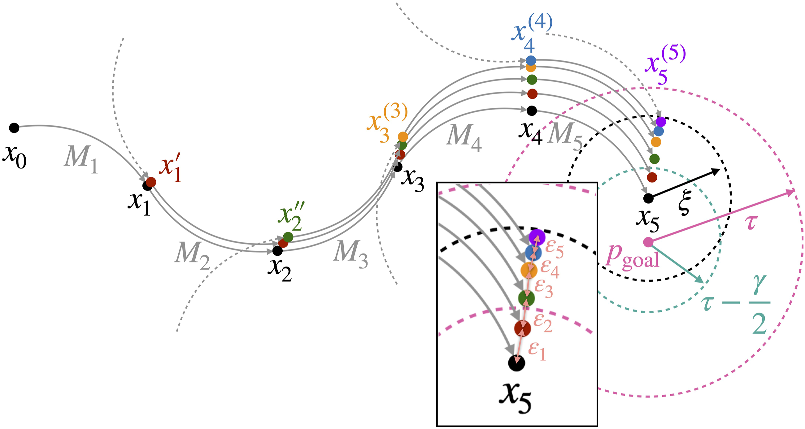${\mathbf{x}}_1^{\prime }$ prunes x₁ is shown as red nodes, the plan after ${\mathbf{x}}_2^{″}$ prunes ${\mathbf{x}}_2^{\prime }$ is shown as green nodes, the plan after ${\mathbf{x}}_3^{\left(3\right)}$ prunes ${\mathbf{x}}_3^{″}$ is shown as yellow nodes, the plan after ${\mathbf{x}}_4^{\left(4\right)}$ prunes ${\mathbf{x}}_4^{\left(3\right)}$ is shown as blue nodes, and the pruning configuration ${\mathbf{x}}_5^{\left(5\right)}$ is shown as a purple node. The solid circular arrows represent elements in $M_{{\sigma }_{\epsilon }}$ , and the dashed circular arrows represent connections to predecessors of the pruning configurations. In this particular example, as long as we guarantee that ‖Proj(x₅) − p_goal‖₂ ≤ τ − γ/2 (σ _ɛ is γ/2-robust) and that $\xi ={\sum }_{i=1}^5\xi \le \gamma /2$ , the resultant plan which ended at ${\mathbf{x}}_5^{\left(5\right)}$ still satisfies the required goal tolerance.

Additionally, we prove that when pruning happens for ${\mathbf{x}}_i^{\left(i\right)}$ , the motion plan constructed with $M_{{\sigma }_{\epsilon }}\left[i,n\right]$ is still collision-free. Denote by σ _ɛ (x_i−1, x _i ) the trajectory segment from x_i−1 and x _i along σ _ɛ . Similarly define $\stackrel{\sim }{\sigma }\left({\mathbf{x}}_{i-1}^{\left(i-1\right)},{\mathbf{x}}_i^{\left(i\right)}\right)$ . We now show that $\stackrel{\sim }{\sigma }\left({\mathbf{x}}_{i-1}^{\left(i-1\right)},{\mathbf{x}}_i^{\left(i\right)}\right)$ is a local ɛ _i -strict approximation of σ _ɛ (x_i−1, x _i ) for ${\epsilon }_i=(L_s^i-1)/(L_s-1)\cdot d_{\text{sim}}$ . To see that, first note that both trajectory segments use the same motion primitive and have the same length. Additionally, $\rho \left({\mathbf{x}}_i^{\left(i\right)},{\mathbf{x}}_i\right)\le (L_s^i-1)/(L_s-1)\cdot d_{\text{sim}}$ . Finally, an intermediate state x′ along the edge is also close to the corresponding state x along the original edge (on σ _ɛ ), since they can be obtained by applying a motion primitive of a shorter length, and Lipschitz continuity of the system guarantees $\rho \left({\mathbf{x}}^{\prime },\mathbf{x}\right)\le (L_s^i-1)/(L_s-1)\cdot d_{\text{sim}}<\gamma /2$ . Since σ _ɛ is γ/2-robust (with ɛ ≤ γ/2), we guarantee that the motion plan $\stackrel{\sim }{\sigma }$ is collision free.

To summarize, as long as the required conditions are satisfied, RCS finds a motion plan.

5.4.3. Resolution optimality of RCS*_D

Similarly to the proof of RCS, we first consider a simplified version of RCS*, termed RCS*_D, which does not use node pruning as part of duplicate detection (Alg. 2, line 9) and later extend it to RCS*. For simplicity, we assume that both RCS*_D and RCS* do not use the additional optimizations described in Section 4.3 or ,4.4 and do not use $\mathcal{C}\left(\text{bestPlan}\right)$ for early pruning, which does not affect the validity of arguments used below.

First, following the discussion in Section 5.4.1, RCS*_D terminates in finite time. Then, to show that Thm. 2 holds for RCS*_D, we consider a reference trajectory σ* and assume that conditions (C1’)-(C3’) are satisfied. According to (C1’), (C2’), and Thm 3, as σ* is decomposable, for some ɛ > 0, there exists a fine resolution R(σ*, ɛ) with which a piece-wise strict ɛ-approximation of σ* can be constructed. We denote such piece-wise strict ɛ-approximation as ${\sigma }_{\epsilon }^{*}$ . Moreover, it holds that $\mathcal{C}\left({\sigma }_{\epsilon }^{*}\right)\le \left(1+k\cdot \epsilon \right)\cdot \mathcal{C}\left({\sigma }^{*}\right)$ , where k = (L _c + c_max)/c_min is as defined in (C2’). Furthermore, we mention that the precise value of ɛ will be assigned later on and for now we only assume that $\epsilon \in (0,\gamma /2]$ .

Similar to the discussion in Section 5.4.1, ${\sigma }_{\epsilon }^{*}$ is at least γ/2-robust given ɛ ≤ γ/2. Thus, for a cutoff resolution R_min that is fine enough, ${\sigma }_{\epsilon }^{*}$ will be explored by the search tree constructed by RCS*_D.

5.4.4. Accounting for pruning in RCS*

The proof for this theorem follows the same idea as Section 5.4.2, so we only focus on cost approximation. Since the optimal trajectory σ* is curvature bounded, there exists some fine resolution R(σ*, ɛ) that can be explored by RCS*, with which we can construct a piece-wise strict ɛ-approximation of σ*. We denote the approximation as ${\sigma }_{\epsilon }^{*}$ and the result found by RCS* as ${\stackrel{\sim }{\sigma }}^{*}$ .

Similar to Section 5.4.2, we denote the sequence of motion primitives that composes ${\sigma }_{\epsilon }^{*}$ as $M_{{\sigma }_{\epsilon }^{*}}=\left\{{\mathcal{M}}_1,\dots ,{\mathcal{M}}_n\right\}$ , and the sequence of configurations along ${\sigma }_{\epsilon }^{*}$ as {x₀, x₁, …, x _n }, where ${\mathbf{x}}_0={\mathbf{x}}_{\text{start}},{\mathbf{x}}_i={\mathbf{x}}_{i-1}\oplus {\mathcal{M}}_i,i\in \left[1,n\right]$ . Following the notion in Section 5.4.2, ${\mathbf{x}}_i^{\left(j\right)},j\le i$ denotes the configuration ${\mathbf{x}}_j^{\left(j\right)}+M_{{\sigma }_{\epsilon }^{*}}\left[j+1,i\right]$ , where ${\mathbf{x}}_j^{\left(j\right)}$ is the configuration along ${\stackrel{\sim }{\sigma }}^{*}$ that replaces ${\mathbf{x}}_j^{\left(j-1\right)}$ .

We now consider the cost of 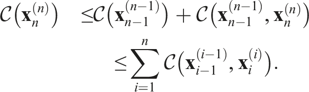${\stackrel{\sim }{\sigma }}^{*}$ . Note that in RCS* we only allow ${\mathbf{x}}_i^{\left(i\right)}$ to replace ${\mathbf{x}}_i^{\left(i-1\right)}$ when $\mathcal{C}\left({\mathbf{x}}_i^{\left(i\right)}\right)\le \mathcal{C}\left({\mathbf{x}}_i^{\left(i-1\right)}\right)$ . Here, $\mathcal{C}\left(\mathbf{x}\right)$ denotes the cost of a node associated with x in the search tree. Thus, for the final configuration along ${\stackrel{\sim }{\sigma }}^{*}$ , we have

$\begin{array}{cc}\mathcal{C}\left({\mathbf{x}}_n^{\left(n\right)}\right)& \le \mathcal{C}\left({\mathbf{x}}_{n-1}^{\left(n-1\right)}\right)+\mathcal{C}\left({\mathbf{x}}_{n-1}^{\left(n-1\right)},{\mathbf{x}}_n^{\left(n\right)}\right)\\ & \le {\displaystyle \sum }_{i=1}^n\mathcal{C}\left({\mathbf{x}}_{i-1}^{\left(i-1\right)},{\mathbf{x}}_i^{\left(i\right)}\right).\end{array}$

It remains to bound the expression $\mathcal{C}\left({\mathbf{x}}_{i-1}^{\left(i-1\right)},{\mathbf{x}}_i^{\left(i\right)}\right)$ for any 1 ≤ i ≤ n. Following the proof of Thm. 1, ${\stackrel{\sim }{\sigma }}^{*}\left({\mathbf{x}}_{i-1}^{\left(i-1\right)},{\mathbf{x}}_i^{\left(i\right)}\right)$ is a local ɛ _n -strict approximation of ${\sigma }_{\epsilon }^{*}\left({\mathbf{x}}_{i-1},{\mathbf{x}}_i\right)$ for ${\epsilon }_n=(L_s^n-1)/(L_s-1)\cdot d_{\text{sim}}<\gamma /2$ . According to the similar-cost property of local strict approximation, we have that

$\mathcal{C}\left({\mathbf{x}}_{i-1}^{\left(i-1\right)},{\mathbf{x}}_i^{\left(i\right)}\right)\le \left(1+k{\epsilon }_n\right)\cdot \mathcal{C}\left({\mathbf{x}}_{i-1},{\mathbf{x}}_i\right).$

where k is as defined in (C2’). To summarize, the accumulated cost of ${\stackrel{\sim }{\sigma }}^{*}$ is as follows:

$\mathcal{C}\left({\mathbf{x}}_n^{\left(n\right)}\right)\le {\displaystyle \sum }_{i=1}^n\mathcal{C}\left({\mathbf{x}}_{i-1}^{\left(i-1\right)},{\mathbf{x}}_i^{\left(i\right)}\right).$

It remains to determine the value of ɛ to achieve a desired approximation factor of 1 + ɛ_cost. So far we required ɛ ≤ γ/2. To further guarantee that $\mathcal{C}\left({\mathbf{x}}_n^{\left(n\right)}\right)\le \left(1+{\epsilon }_{\text{cost}}\right)\cdot \mathcal{C}\left({\sigma }^{*}\right)$ holds, we require that ɛ ≤ (2ɛ_cost − k · γ)/(k(2 + k · γ)). Thus, we take ɛ = min{γ/2, (2ɛ_cost − k · γ)/(k(2 + k · γ))}. According to condition (C3’), it follows that γ ≤ ɛ_cost/k, so we always have ɛ > 0.

To summarize, as long as the required conditions are satisfied, RCS* still finds a valid motion plan σ that satisfies $\mathcal{C}\left(\sigma \right)\le \left(1+{\epsilon }_{\text{cost}}\right)\cdot \mathcal{C}\left({\sigma }^{*}\right)$ .

6. Experiments

We evaluate our new motion planners for steerable needles using scenarios based on the medical tasks of lung biopsy and liver biopsy:

(i) Lung biopsy: Lung cancer is the deadliest form of cancer in the United States, killing over 130,000 Americans each year according to American Cancer Society (2022). Early diagnosis is critical for patient survival, and biopsy of suspicious nodules is required for diagnosis. Steerable needles deployed from bronchoscopes have the potential to safely and accurately reach nodules throughout the lung for biopsy and localized treatment (Kuntz et al., 2016; Swaney et al., 2017). In this procedure, the steerable needle is deployed from a bronchoscope inside the lung and must steer from the start pose just outside a bronchial tube (the furthest pose reachable by the bronchoscope) to the nodule while avoiding anatomical obstacles that include the large blood vessels, the bronchial tubes, and the lung boundary.

(ii) Liver biopsy: Liver cancer accounts for roughly 840,000 new cancer cases and 780,000 cancer-related deaths each year worldwide. It is more prevalent in countries in sub-Saharan Africa and Southeast Asia than in the US and is one of the few cancers whose death rates are still on the rise (Bray et al., 2018). Similar to lung cancer, early diagnosis is key with one tool being biopsy of suspicious nodules. In liver biopsy procedures, the steerable needle is deployed through the surface of the liver and must steer from the start pose near the liver surface to the nodule while avoiding anatomical obstacles including large blood vessels.

The CT scans used in both experiments are from The Cancer Imaging Archive (TCIA) (Clark et al., 2013), a public medical image repository for cancer studies. The chest CT scan for lung biopsy scenario is from the Lung Image Database Consortium and Image Database Resource Initiative (LIDC-IDRI) image collection (Armato et al., 2011, 2015), while the abdomen CT scan for liver biopsy scenario is from the CT volumes with multiple organ segmentations (CT-ORG) dataset (Rister et al., 2019) We illustrate in Figure 1 (top) volumetric models of the relevant anatomy segmented from a CT scan. For the lung segmentation, we follow the method described in Fu et al. (2018). For the liver segmentation, we use the segmentation labels from the CT-ORG dataset for the liver region. The major blood vessels are also segmented using the method described in Fu et al. (2018).

6.1. Test case generation

To create test cases for planning, we randomly sample 50 collision-free start configurations for each scenario, and for each start configuration, we sample 10 collision-free goal points uniformly inside the kinematically forward-reachable workspace of the needle. Since we consider two different values for κ_max (see Section 6.2), for each start configuration, two different sets of goal points are sampled. This is because with a larger κ_max, the kinematically forward-reachable workspace would also be larger. Thus, each scenario has 1000 test cases in total, including 500 cases for each needle design.

More specifically, in the lung biopsy scenario, start configurations are sampled along the bronchial tube walls (i.e., points reachable by the bronchoscope from which the steerable needle can be deployed), and the goal points are sampled in the lung parenchyma (i.e., points in the tissue of the lung outside the bronchial tubes in which nodules requiring biopsy may occur). In the liver biopsy scenario, start configurations are sampled near the anterior surface of the liver (i.e., points where the liver is close to the abdomen skin from which the steerable needle can be deployed), and the goal points are sampled in the liver tissue (i.e., points in the tissue of the liver in which nodules requiring biopsy may occur). See Figure 12 for the scenarios and representative plans computed by RCS.

Figure 12.

Visualization of the anatomical environments and 10 representative plans for each scenario computed by 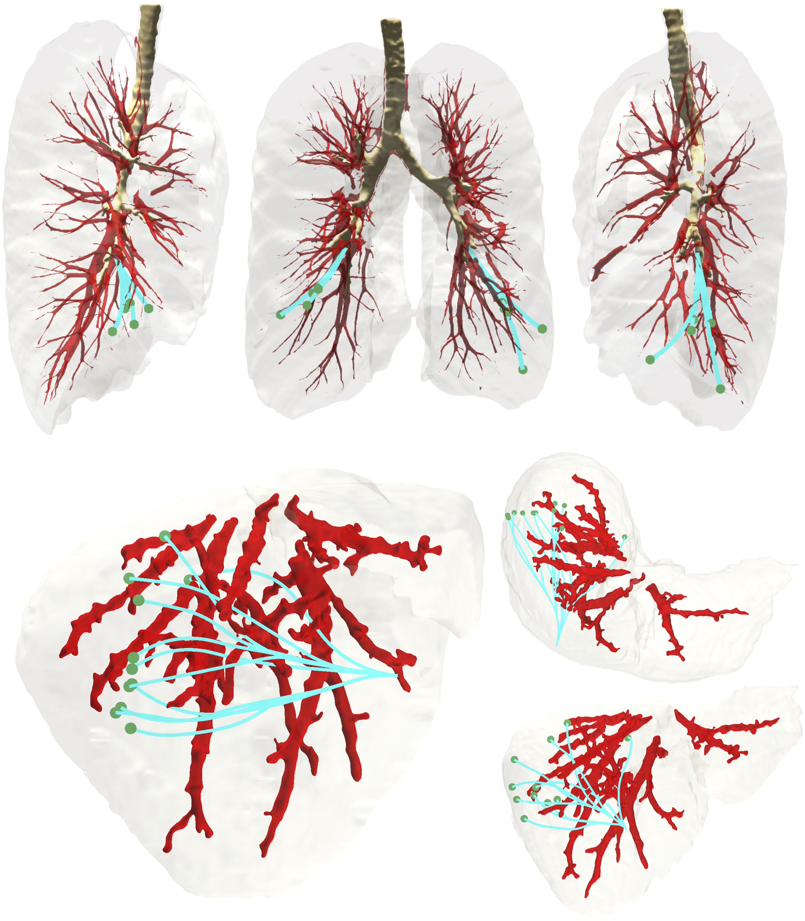RCS (cyan). Top and bottom figures depict three views of the lung environment and the liver environment, respectively. In all figures, the needle steers to targets (green) while avoiding anatomical obstacles including major blood vessels (red) and the lung or liver boundary (gray). In the top figure, bronchial tubes are depicted in brown.

To avoid skewing the data with trivial test cases, we discarded test cases where the start configuration can be connected directly to the goal point with a collision-free arc. Additionally, we use inevitable collision check (mentioned in Section 4.3) to disallow cases where the start configuration has an inevitable collision deeming the problem unsolvable. Finally, note that it is not guaranteed that a valid plan exists for a test case.

6.2. Setups

We consider a steerable needle with two different maximum curvatures κ_max = (100 mm)⁻¹ and (50 mm)⁻¹, both with a device diameter of 2 mm and maximum insertion length of 80 mm. The simulated workspace was reconstructed from preoperative CT scans where ${\mathcal{W}}_{\text{obs}}$ is a point cloud representing the anatomical obstacles described above. We use a collision-checking resolution of 0.5 mm and a goal tolerance of τ = 1.0 mm.

We compare in simulation RCS and RCS* with several other steerable needle planners:

(i) RRT: The RRT-based needle planner (Kuntz et al., 2015; Patil et al., 2014) with 5% goal biasing and 100% goal-connecting ratio.

(ii) AO-RRT : AO-RRT (Hauser and Zhou, 2016; Kleinbort et al., 2020) adapted for steerable needles, with maximum rotation control of 2π and a maximum insertion control of 16 mm. We follow the guidelines in Kleinbort et al. (2020) for cost sampling and distance weighting between the configuration space and cost space. For a fair comparison, we use the same goal-connecting method as RRT.

(iii) AFT: The AFT-based needle planner (Liu et al., 2016; Pinzi et al., 2019), with setup following Pinzi et al. (2019). Adaptive Fractal Tree internally uses a hybrid cost function to choose the plan to optimize in the next iteration; we use ${\mathcal{C}}_{\text{hybrid}}\left(\sigma \right)=\omega \cdot \mathcal{C}\left(\sigma \right)+{\Vert \sigma \left(l\right)-p_{\text{goal}}\Vert }_2/\tau$ , where ω is a weighting parameter depending on the scale of $\mathcal{C}$ . Note that ${\mathcal{C}}_{\text{hybrid}}$ is only used internally in AFT while $\mathcal{C}$ is always used for performance comparison across different planners.

For our proposed planners RCS and RCS*, we have δℓ_max = 16 mm and the system cutoff resolution is computed for control frequency 40 Hz, which corresponds to a time interval of 0.025s: δℓ_min = 5(mm/s) · 0.025s = 0.125 mm, δθ_min = 2π(rad/s) · 0.025s ≈ 0.157 rad. The value of insertion and rotation velocities is taken from Rucker et al. (2013) and the control frequency is the measurement rate of the NDI Aurora tracking system (Northern Digital, 2022). Additionally for RCS*, we use a lookahead value of n_la = 3, and for all cost functions, we set the approximation parameter to be ɛ_cost = 0.1. Other system constants (e.g., L _s ) are empirically determined.

We also ran a search-based planner denoted as SINGLE_RES that includes all optimizations of RCS mentioned in Section 4.3 or 4.4 but that uses only the finest resolution (with no multiple resolutions).

All experiments were run on a dual 2.1 GHz 16-core Intel Xeon Silver 4216 CPU and 100 GB of RAM. All parallelizations were implemented with Motion Planning Templates (MPT) (Ichnowski and Alterovitz, 2019). All parallelized versions (including RRT and AO-RRT) use 60 threads. Code for our proposed planners is available on GitHub (Fu et al., 2021a).

6.3. Success rate comparison

We now present results pertaining to the success rate of the different algorithms. In our setting, the success rate is the ratio of solved cases among the set of 500 test cases. All planners other than AFT were allowed 100 s. As for AFT, while the original AFT algorithm is GPU accelerated, here we present results for our CPU-based implementation and only focus on the feasibility of the method and not on the computation times (we let AFT run until it finishes three iterations as suggested in Liu et al. (2016)). For planners that require a cost function $\mathcal{C}$ as input (i.e., AO-RRT, AFT, and RCS*), we used trajectory length as the cost function when comparing success rate. Since the hybrid cost function in AFT does not necessarily favor paths with minimal goal tolerance and thus may affect its success rate, we set the weighting parameter ω = 0 for success rate analysis. In RCS*, the plan obtained keeps being updated (Alg. 2 line 11) and only the minimal-cost plan is returned. To fairly compare success rate, the ability to find any valid (not necessarily optimal) plan, we consider RCS* to succeed as long as it finds a plan (bestPlan ≠ NULL).

The results are shown in Figure 13. First, among RCS variants, RCS_S performed much better than RCS_B (see Table 1 for details about these variants), indicating the three domain-specific optimizations introduced in Section 4.3 dramatically improved the efficiency of the algorithm. Furthermore, except for the slight overhead affecting the early stage of the planner $\left(<50\text{ms}\right)$ , RCS achieved even better performance than RCS_S. Moreover, RCS* showed similar performance as RCS. The single-resolution planner, SINGLE_RES, achieved low success rates $\left(<40\%\right)$ , suggesting that the multi-resolution approach in RCS variants is necessary for high performance. Second, the single-threaded RCS_S achieved better performance than the single-threaded RRT_S, comparable to and often with higher performance than the multi-threaded RRT, and always with higher performance than the multi-threaded AO-RRT. AO-RRT, although outperforming RRT in the early stage $\left(<0.1\mathrm{s}\right)$ , showed slow convergence in the later stages of the search. From the perspective of computation time, RCS and RCS* in general solved over 75% of the test cases within a second and were over 100× faster in reaching RRT’s final success rate (at 100 s). When looking at each test case, RCS and RCS* on average took only 42.2% of the computation time spent by RRT, indicating they were roughly 2.4× faster than RRT. Similarly, RCS and RCS* were on average 1.5× faster than AO-RRT on a per-case perspective. Adaptive Fractal Tree achieved a success rate of between 55% and 75%, which was significantly lower than that of RCS and RCS*, with many of the failures due to the computed trajectories not satisfying the maximum-allowed targeting error of τ = 1 mm. From the perspective of the final success rates, RCS and RCS* were on average 5.4% higher than RRT, 7.2% higher than AO-RRT, and 23.1% higher than AFT.

Figure 13.

Success rate as a function of computation time. All plots use logarithmic time axes.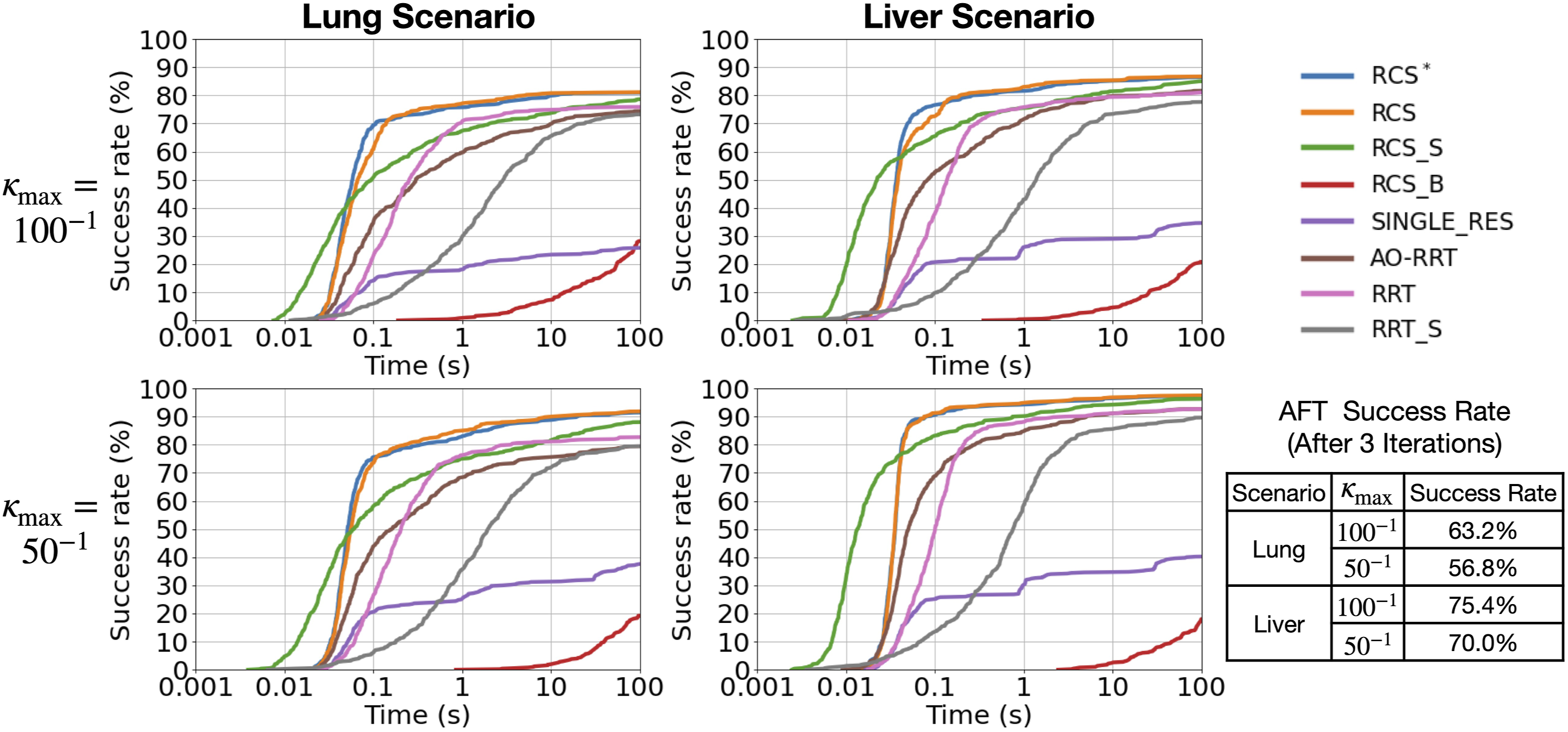

6.4. Plan quality comparison

We continue to compare plan qualities, considering three different well-behaved cost functions:

(i) Trajectory length: $\forall \mathbf{x}\in \mathcal{X},c\left(\mathbf{x}\right)=1$ . This cost function is by nature well-behaved given c_min = c_max = 1, L _c = 0.

(ii) Cost map: this cost function is informed by a cost map derived from medical images (Fu et al., 2018), where each voxel in the 3D cost map is associated with a cost value that represents tissue damage. We forced c_min = 0.01 and then used trilinear interpolation to smooth out the voxelized cost map to make it well-behaved.

(iii) Obstacle clearance: Cost function ${\int }_0^{\ell }\text{cl}\left(\sigma \left(s\right)\right)$ ^-1ds, where cl(·) is the clearance from obstacles, has been widely used (Agarwal et al., 2018; Kuntz et al., 2015; Strub and Gammell, 2021; Wein et al., 2008) since it captures both trajectory length and clearance from obstacles. Here, we modify the point-based cost to be c(x) = min{cl(x)^-1, c_max}, forcing the cost not to exceed c_max = (0.1 mm)⁻¹ to make it well-behaved.

For the lung biopsy scenario, we considered the cost functions of trajectory length and cost map (i.e., costs (i) and (ii), above). In contrast, for the liver biopsy scenario, we considered the cost functions of trajectory length and obstacle clearance (i.e., costs (i) and (iii), above). This is because the method for constructing a cost map in Fu et al. (2018) was designed specifically for the lung anatomy where plenty of small blood vessels exist. For liver anatomy, the cost map constructed using the same method is far less informative.

For this set of experiments, we only evaluated RCS*, RCS, RRT, AO-RRT, and AFT. All four planners except AFT were parallelized and were allowed 10 s, while we allowed AFT to finish three iterations. To compare how plan quality is improved as more computation time is given, we kept track of the best plan found by each planner at each time stamp.

For all cost functions, the cost of a plan may vary significantly between test cases. For example, trajectory length is affected by how far away the target lies relative to the start pose and cost map values are much higher when the needle is steering in a vessel-cluttered region. Instead of averaging across different test cases directly, for each test case, we compute the relative cost using the RCS* as a reference. More specifically, for a given time step, the relative cost is valid if both the target planner and RCS* have successfully found a plan and the value of the relative cost is computed by ${\mathcal{C}}_{\text{relative}}={\mathcal{C}}_{\text{target}}/{\mathcal{C}}_{\mathsf{R}\mathsf{C}\mathsf{S}\mathsf{*}}$ . We then averaged across all test cases with a valid relative cost for each time step.

The results are shown in Figure 14. We start our analysis by considering the trajectory length. For all four corresponding plots (for both the lung and liver and for both needle curvatures), the relative costs mostly lie between a factor of 1.01× and 1.04× the cost obtained via RCS*, with RCS* outperforming all other planners. Additionally, the relative cost is flatter for κ_max = (100 mm)⁻¹ compared to (50 mm)⁻¹, indicating that the more flexible the needle is, the greater room for improvement there is. Thus, as needles that are more flexible would be developed, the relative advantage of our method would increase. To understand why the improvement here is relatively low, consider any bounded-curvature trajectory that is 80 mm long (the maximum insertion length). Here, the theoretically minimum Euclidean distance between the two ends is 77.88 mm and 71.74 mm for a radius of curvature κ_max = (100 mm)⁻¹ and (50 mm)⁻¹, respectively. Thus, the upper bounds for the relative cost are 1.027 and 1.115, respectively.

Figure 14.

Plan quality comparisons. Without specification, a plot shows the relative cost (vertical axis) as a function of computation time (horizontal axis), where the time axis is logarithmic, solid lines show the average relative cost when compared to 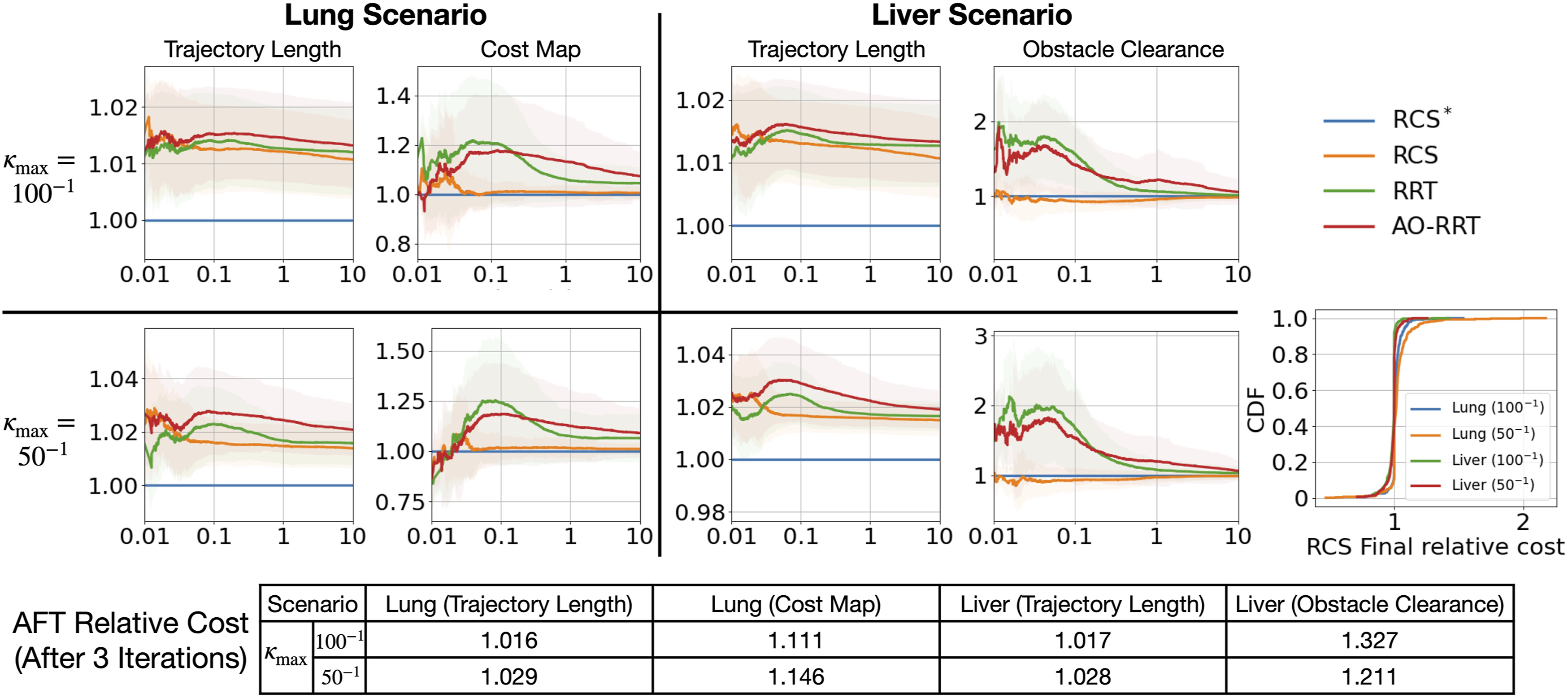RCS*, and shaded regions show the corresponding standard deviation. The final costs for AFT (shown relative to RCS*) are provided in the table. We also include a detailed comparison of RCS and RCS* for the cost metrics that are not trajectory length (i.e., cost map for lung scenario and obstacle clearance for the liver scenario), shown as a cumulative distribution function (CDF).

We continue our analysis by considering the cost map (representing tissue damage) evaluated in the lung scenario. Here, RCS* and RCS showed a larger advantage over RRT and AO-RRT, achieving between 4.5% and 25% lower cost on average. Interestingly, RCS quickly achieved a relative cost that is only slightly higher than 1.0, indicating that its cost is comparable to the cost of RCS*. We also see that RRT was able to improve its path quality but since this is not optimized directly by the algorithm, the relative cost was not improved further. Finally, for AO-RRT, although being asymptotically optimal, its convergence rate was relatively slow and achieved a final cost (at 10s) which was higher than RRT’s.

We finish this part of the analysis by considering the obstacle clearance, evaluated on the liver scenario. Here, RCS and RCS* still outperform RRT and AO-RRT. However, in the early stage of the search (i.e., for $<1\mathrm{s}$ ), RCS achieved better costs than RCS* (relative cost being less than 1.0). A possible explanation is that RCS can better explore different plans with different cost values in the early stage of the search because of its less-strict duplicate detection. As more running time was given, RCS*, with its resolution optimality and with the help of its heuristic (see Strub and Gammell (2021)), was able to improve the cost of paths and the two methods achieved comparable cost at 10 s. Here, we also see that RRT and AO-RRT achieve relatively low costs, compared to other cost metrics. This could be because the cost function is dominated by points that get very close to the obstacles. Thus, a planner achieves a low cost as long as it is able to find a plan with these “good” dominating points.

We notice that RCS and RCS* achieved comparable costs, indicating that RCS, even without optimality guarantees, was performing well in practice for our highly constrained test scenarios. On the other hand, for RCS* to guarantee resolution optimality, it needed to be much more conservative, considering the cost metric properties for worst cases and exploring all potentially better branches in the search tree. From the accumulative distribution function (CDF) plot in Figure 14, we see that RCS* achieved equal or better costs (at 10s) than RCS for 90% of the cost map cases and for 70% of the obstacle clearance cases.

Finally, we also report the final relative cost for AFT in Figure 14. Since AFT’s design addresses both finding a path and optimizing a given cost via one hybrid cost function ${\mathcal{C}}_{\text{hybrid}}$ , it treats the targeting error as a part of ${\mathcal{C}}_{\text{hybrid}}$ and may sacrifice the cost function $\mathcal{C}$ for a lower targeting error. Thus, we can see that AFT had the highest relative cost among all planners.

6.5. Heuristic balancing in RCS and RCS*

In this section, we depict how our algorithms are affected by different parameter choices. We start by evaluating how our definition of rank (equation (4)) affects the behavior of RCS and then continue to evaluate the effect that the lookahead has on the behavior of RCS*.

6.5.1. Evaluating the effect of rank on RCS

Recall that the rank of a node (equation (4)) allows RCS and RCS* to balance between refining the resolution used in a parent node and expanding a node. Roughly speaking, the former corresponds to creating finer motions that make small progress toward the goal but create higher quality paths or better avoid obstacles while the latter corresponds to using coarser motions to make bigger steps toward the goal.

To depict this tradeoff, we consider the cost map metric for lung biopsy and evaluate RCS for a refined rank function using two new parameters a and b:

$\text{Rank}\left(v\right)=\text{Rank}\left(v.\text{parent}\right)+a\left(l_{\ell }\left({\mathcal{M}}_v\right)+l_{\theta }\left({\mathcal{M}}_v\right)\right)+b.$

Results, depicted in Figure 15, demonstrate that if resolution refinement is not penalized (a = 0), all resolutions are treated equally without prioritizing the coarse resolution, and both the success rate and plan quality are negatively affected. This suggests that using multiple resolutions is important and we should prioritize coarse resolutions.

Figure 15.

Comparing the performance of 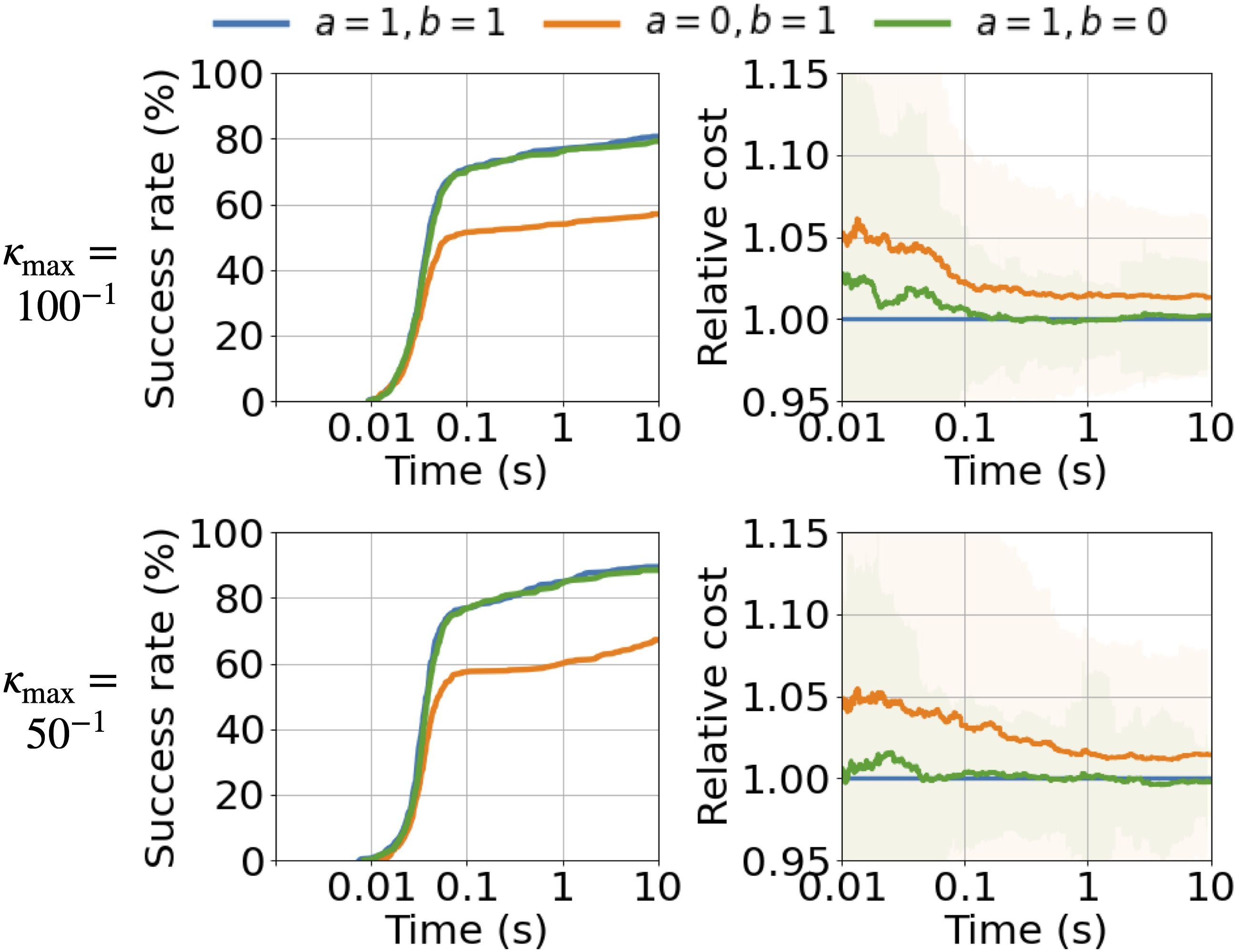RCS for different rank definitions (i.e., parameter values a and b) on the lung biopsy scenario with the cost map metric.

6.5.2. Evaluating the effect of the lookahead on RCS*

Recall that in RCS*, a secondary heuristic f(·) is used to guide the search, and the lookahead parameter n_la is used to balance between a node’s rank and f(·). Having a large n_la value allows RCS* to prioritize nodes with potentially lower cost, but as the rank plays a less important role, the benefits of the multi-resolution framework are weakened and it may take longer to find solutions (although with higher quality).

To depict this tradeoff, we consider again the cost map metric for lung biopsy and evaluate RCS* for different lookahead values (Figure 16). We see that when n_la is increased from 0 to 3, the success rate hardly changed. However, when n_la = 10, RCS* achieved lower success rate between 0.05 and 5 s. When pushing this to the limit and taking a value of n_la = 100, RCS* struggled to improve the success rate after 0.1 s, indicating that after solving the easy-to-solve scenarios, RCS* cannot efficiently find solutions for a harder problem using this lookahead. This is because the larger n_la is, the more similar RCS* is to a basic A* search that heavily relies on f(·).

Figure 16.

Comparing the performance of 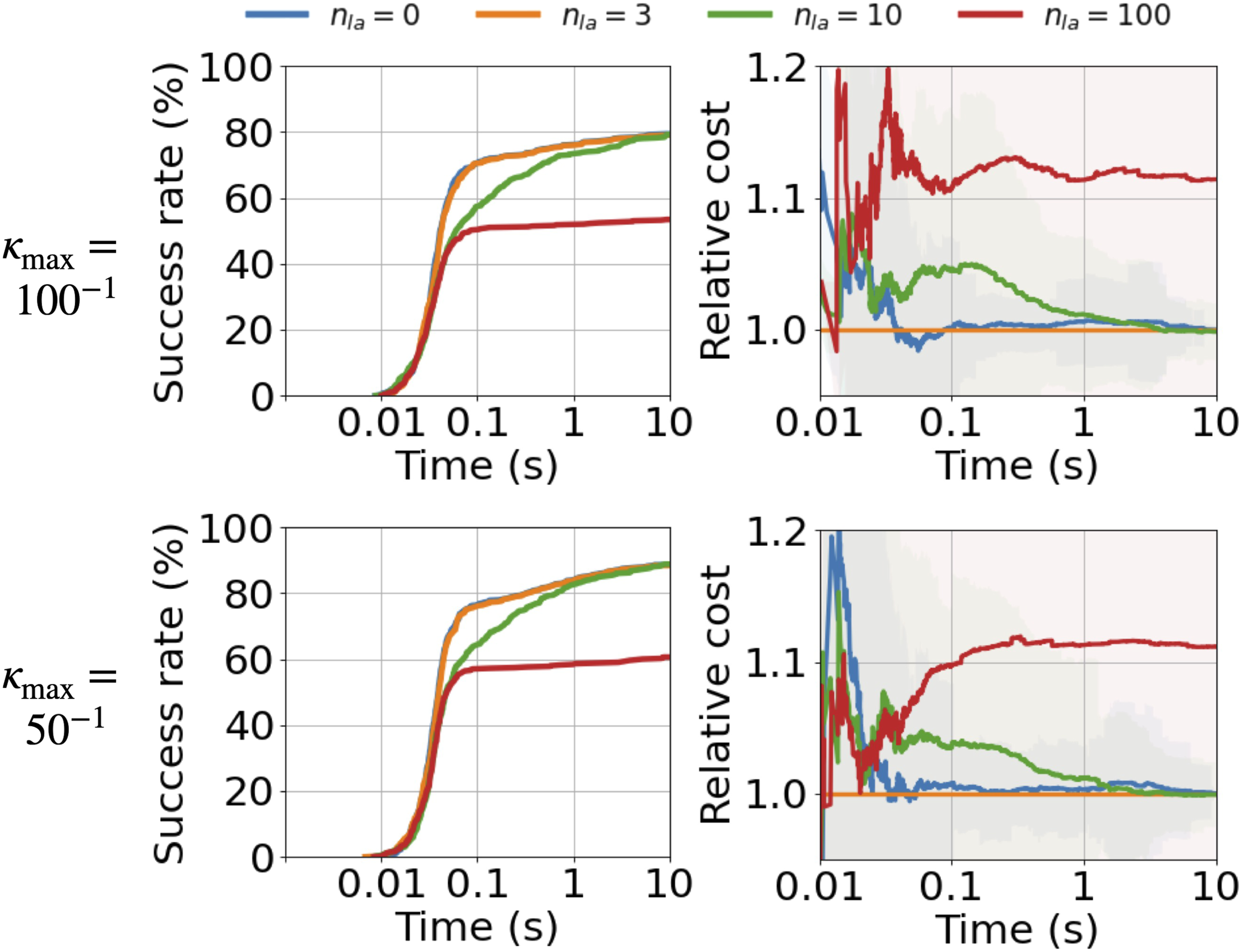RCS* for lookahead parameters on the lung biopsy scenario with the cost map metric.

When it comes to plan quality, we see that RCS* with a lookahead value of n_la = 10 achieved higher cost values in the early stages of the search but was able to converge quickly to match the other variants. However, when taking this to the extreme and using larger lookahead values (n_la = 100), the slowdown is too big and RCS* was not able to efficiently find low-cost solutions.

To summarize, this experiment shows, from another perspective, that the multi-resolution framework is important both for efficiency and as a general heuristic without considering a specific cost function. As a general guideline, we need to keep n_la not too large to retain the benefits of prioritizing coarse resolutions. In our settings, we choose n_la = 3 which proved to adequately balance the success rate and the ability to improve the overall plan quality.

7. Conclusion

In this paper, we took an important step toward creating a certifiable optimal motion planner for steerable needles. Specifically, we introduced a resolution complete motion planner for steerable needles, RCS, and an extended version, RCS*, that is also resolution optimal. We provided formal proof to show that, under some mild assumptions on the system and the solution, RCS is guaranteed to find in finite time a plan as long as the problem admits a qualified motion plan. RCS* is guaranteed to find in finite time a plan whose cost can be as close as desired to the globally optimal qualified motion plan. We also showed that our proposed planners outperform state-of-the-art needle planners in clinically realistic simulations considering clinically relevant cost functions by achieving higher success rates, lower computation times, and higher plan qualities.

We view this work as an algorithmic foundation required to obtain certifiable optimal motion planning for steerable needles. Our planner is the first planner for steerable needles that guarantees resolution completeness and resolution optimality, but more work remains.

(i) Our analysis showed that, under some mild assumptions, when a qualified solution exists, if the cutoff resolution is fine enough and the plan is robust to some degree (i.e., has some clearance from the obstacles and the goal region boundary), the algorithms will find it. However, it would be valuable for medical applications to provide the precise relation between the system’s controls and this cutoff resolution. Subsequently, we need to provide the precise relation between this cutoff resolution (i.e., what does it mean to be “fine enough”) and the clearance of plans (i.e., what should “some clearance” be?). In the ideal case, when a desired clearance is given (e.g., say we do not consider plans that get overly close to obstacles as a reference plan to approximate), we should be able to provide a cutoff resolution, in an explicit form, that guarantees resolution completeness and resolution optimality. Future work will use this foundation to compute the relation between the aforementioned parameters in order to give physicians certifiable software for motion planning for steerable needles.

(ii) Although our proposed steerable needle planners showed good efficiency in experiments, the worst-case computation time can be long. We will also investigate techniques to further speed up the planners (e.g., GPU acceleration or additional optimizations for effective early pruning).

(iii) We have started experimentally evaluating the planner with steerable needles in ex-vivo animal tissues. We also will explore how these certifiable guarantees can help gain the trust of physicians for autonomous medical robots.