
Abstract
Continuum robots have the potential to enable new applications in medicine, inspection, and countless other areas due to their unique shape, compliance, and size. Excellent progress has been made in the mechanical design and dynamic modeling of continuum robots, to the point that there are some canonical designs, although new concepts continue to be explored. In this paper, we turn to the problem of state estimation for continuum robots that can been modeled with the common Cosserat rod model. Sensing for continuum robots might comprise external camera observations, embedded tracking coils, or strain gauges. We repurpose a Gaussian process (GP) regression approach to state estimation, initially developed for continuous-time trajectory estimation in SE(3). In our case, the continuous variable is not time but arclength and we show how to estimate the continuous shape (and strain) of the robot (along with associated uncertainties) given discrete, noisy measurements of both pose and strain along the length. We demonstrate our approach quantitatively through simulations as well as through experiments. Our evaluations show that accurate and continuous estimates of a continuum robot’s shape can be achieved, resulting in average end-effector errors between the estimated and ground truth shape as low as 3.5 mm and 0.016° in simulation or 3.3 mm and 0.035° for unloaded configurations and 6.2 mm and 0.041° for loaded ones during experiments, when using discrete pose measurements.
1 Introduction
Continuum robots are actuatable, compliant structures, whose constitutive material forms curves with continuous tangent vectors. The motion capabilities of continuum robots can be expressed by a set of motion primitives (extension/contraction, bending, shear, and twisting) that are realized in concatenated segments composing the robot. The compliance inherent in the continuum structure allows the robot to adapt to contact with its environment and to compensate for the limitations in its actuatable degrees of freedom. At small diameters and high lengths, continuum robots show great potential for manipulation in constrained environments such as medical (Burgner-Kahrs et al., 2015) and industrial applications, for example, in-situ inspection, maintenance, and repair (Dong et al., 2019; Wang et al., 2021).
We have seen significant advancements on how to effectively design and actuate small-scale continuum robots over the past two decades (Webster, and Jones, 2010; Walker, 2013). In order to efficiently plan and control motions of these manipulators, usually accurate models are required. While the modeling accuracy achieved by the most sophisticated approaches for continuum robots is promising (Rucker et al., 2010; Rucker and Webster, 2011), non-negligible discrepancies between model predictions and robot prototypes persist, largely due to unmodeled effects. As these inaccuracies make accurate control and motion planning challenging, sensors are used to infer information about the robot’s actual state. In continuum robotics research, we predominantly use discrete position or pose information, usually obtained from external cameras (Hannan and Walker, 2005) or embedded electromagnetic tracking coils (Mahoney et al., 2016), as well as discrete strain information, obtained from embedded fiber Bragg grating sensors (Modes et al., 2021). An overview of different shape sensing techniques for continuum robots, focusing on their possible application in minimally invasive surgery, is provided by Shi et al. (2017). Mahoney et al. (2018) emphasize that sensing is a crucial component in the deployment of continuum robots, being fundamentally coupled to their design, motion planning, and control. Therefore, special attention should be given to accurately estimating the state of continuum robots based on sensor readings.
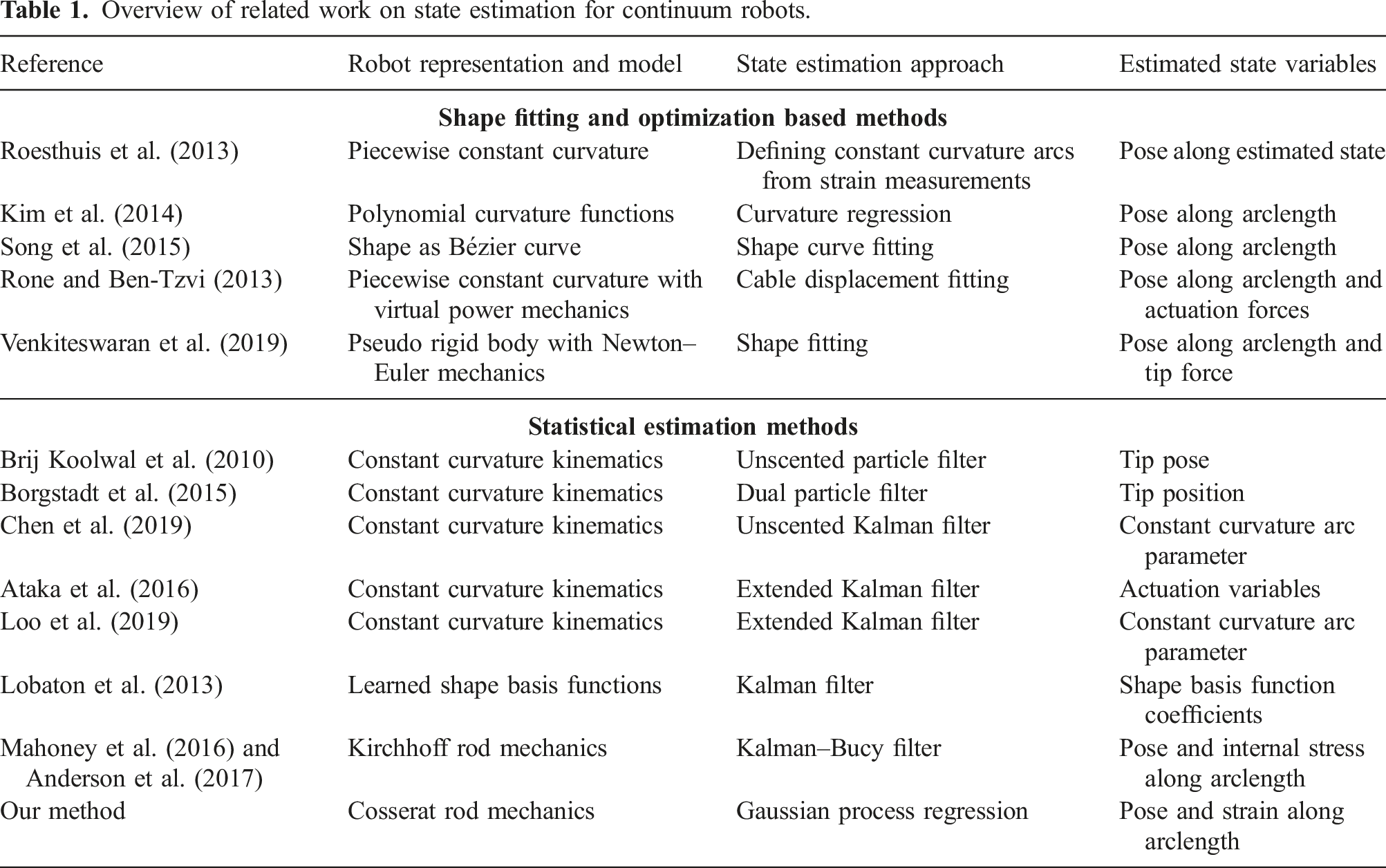
One commonly used approach to infer information about a continuum robot’s shape is to use optimization methods to fit a given shape representation to discrete sensor observations. This can either mean fitting the parameters of a mechanics-based kinematic model to align the modeled shape with external sensor information or directly fitting shape representation functions, such as polynomials or other continuous curves to the discrete sensor readings. Examples include shape estimation approaches utilizing models based on the principle of virtual power (Rone and Ben-Tzvi, 2013) and pseudo rigid-body assumptions (Venkiteswaran et al., 2019), as well as finding Bezier curves (Song et al., 2015), polynomials (Kim et al., 2014), or constant curvatures (Roesthuis et al., 2013) that match the measurements. While these approaches make it possible to reason about the shape of the continuum robot, sensor noise as well as modeling uncertainties are not explicitly taken into account. Thus, more sophisticated stochastic state estimation approaches based on statistical methods are desirable.
The majority of approaches that apply statistical methods to estimate the robot’s end-effector pose or shape are based on simplified kinematic models that assume bending in constant curvatures. Examples include shape estimation of catheters (Brij Koolwal et al., 2010; Borgstadt et al., 2015), tendon-driven continuum robots (Chen et al., 2019; Ataka et al., 2016), and soft robots (Loo et al., 2019). In another approach, Lobaton et al. (2013) incorporate a more general shape representation, consisting of a combination of spatial basis functions, with a stochastic state estimation approach. All of these approaches provide filtered and robust estimates of the robot’s shape given noisy sensor data. However, due to the simplified geometrically motivated assumptions, their estimated state is restricted to only include the position and orientation of the robot’s shape. Thus, it does not include internal strains, which could be used to gain insights into the robot’s internal forces and moments as well as to estimate external loads. A more complete state representation of continuum robots to be used in stochastic state estimation approaches is proposed by Mahoney et al. (2016). In their work, the state of a continuum robot is based on a differential formulation, allowing to represent more sophisticated mechanics-based kinematic models. Based on this state representation, an estimation approach utilizing a Kalman–Bucy filter in combination with a Rauch–Tung–Striebel smoother is proposed. The approach is applied to a concentric tube continuum robot and a parallel continuum robot setup in Anderson et al. (2017), using a Kirchhoff rod modeling approach in both cases.
Following a similar approach, we are proposing a general state estimation method for continuum robots that can be modeled using Cosserat rod theory. The proposed state estimation approach is based on a sparse Gaussian process regression, a method previously applied to continuous-time trajectory estimation in
Overview of related work on state estimation for continuum robots.
Thus, the main contribution and novelty of our work are its versatility, allowing it to be applied to any Cosserat rod type continuum robot, and its potential for computational efficiency.
2 Theory
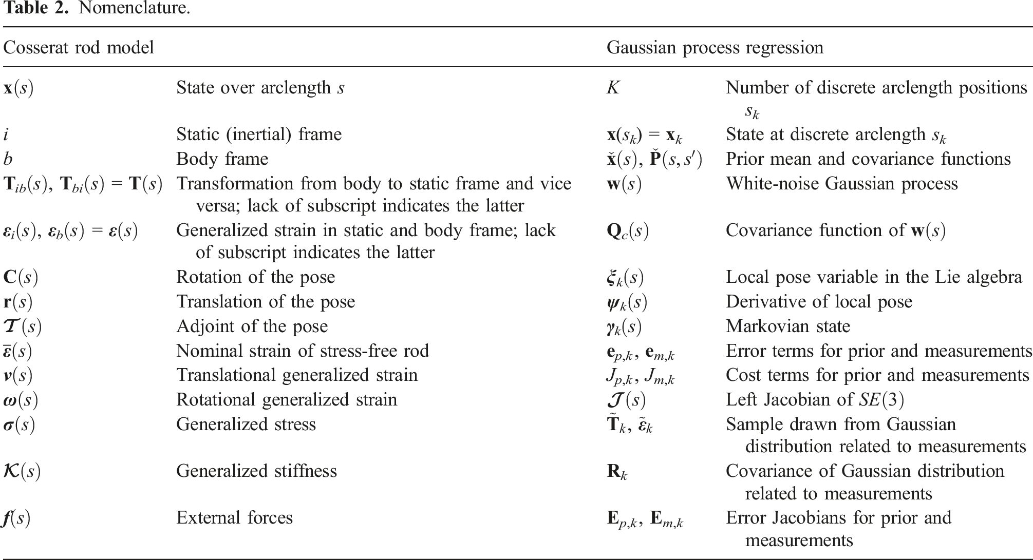
Nomenclature.
2.1 Cosserat rod model
We seek a reasonable model of the physics of a continuum robot to serve as our prior for state estimation. The well-known Cosserat rod model, commonly employed in continuum robotics (Rucker and Webster, 2011; Rao et al., 2021), serves the purpose. Simplifications of the Cosserat rod are commonly employed in the graphics community (Pai, 2002), and we will leverage a similar version here.
Figure 1 notes the similarity of the Cosserat rod model to the dynamics of a rigid body, when expressed in Comparison of the equations of motion (parameterized by time) of a rigid body (D’Eleuterio, 1985) to those of the quasi-static Cosserat rod model (parameterized by arclength) (Pai, 2002). Quantities are expressed in the body frame and 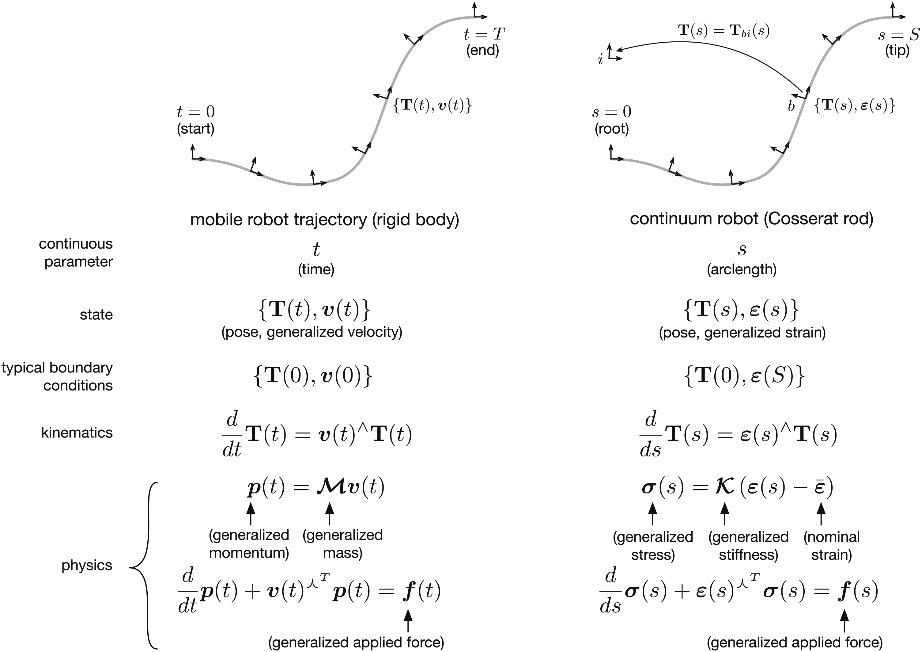
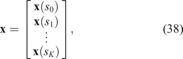
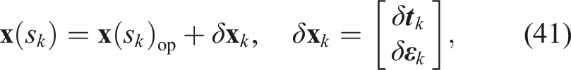
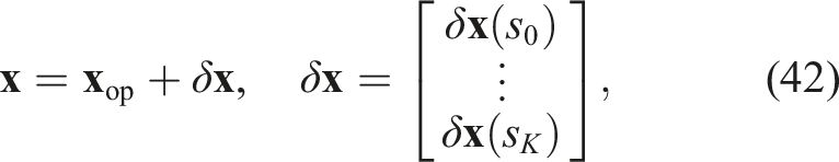
We consider the state of the continuum robot to be
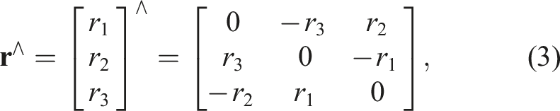
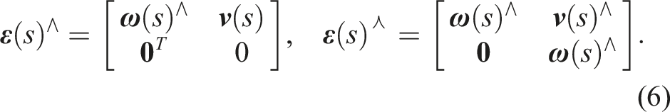
At times, we will also require the adjoint of the pose, 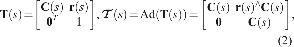
We can further decompose the generalized strain into its translational, 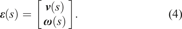
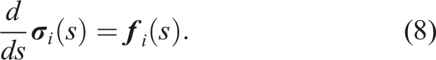
It is worth noting that the analogue of the generalized strain in the continuous-time case is generalized velocity; here, we must think of it as how quickly each component of the pose is changing as we proceed along the length of the rod.
We can relate the pose to generalized strain through the spatial kinematics equation
Intuitively, if the strain is known, we can integrate from the root of the robot to the tip to determine the pose along the length.
The physics equation (i.e., involving forces) requires a bit more explanation. In an inertial (i.e., stationary) frame, i, the generalized stress can be obtained using the constitutive law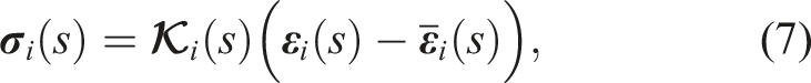
The trouble with writing this in the inertial frame is that the stiffness and nominal strain depend on the configuration of the robot, 
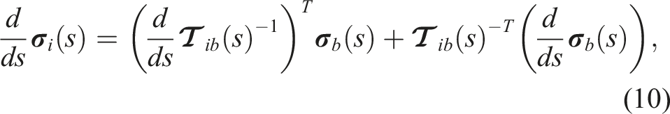
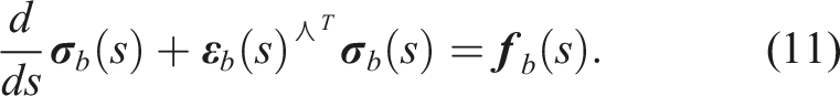
Dropping all frame subscripts, we have the following for the physics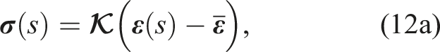
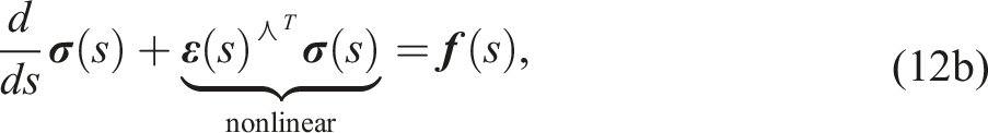
Together, the kinematics (5) and physics (12) constitute our model of a continuum robot that we seek to use to regularize our state estimation problem. The next section introduces the state estimation approach.
2.2 Gaussian process regression for
In this section, we will repurpose the batch continuous-time state estimation framework first described by Barfoot et al. (2014) and later made specific to
2.2.1 Prior
Ideally, our GP prior would take the form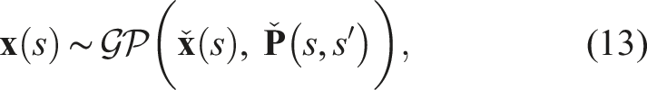
Towards this end, the kinematics (5) and physics (12) from the previous section can be simplified as follows. First, the physics can be written as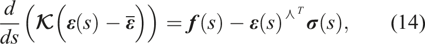
or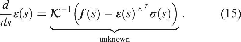
We take the fairly extreme position for now that the right hand side of (15) is unknown, and as such, we will replace it with a white-noise process, resulting in the following model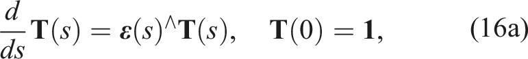
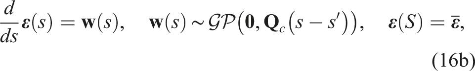
The challenge with (16) is that while our simplifications have made the differential equation for the physics linear, the kinematics remain nonlinear, which is necessary to allow for large robot displacements. This makes it fairly difficult to stochastically integrate these models to produce a prior of the form requested in (13). To overcome this problem, we will employ the same approach as Anderson and Barfoot (2015); Anderson (2016) by using a series of local GPs that are stitched together. Figure 2 depicts the idea. We start by selecting K arclengths, s
k
, along the robot length at which we initialize each of these local GPs. We define local pose variables in the Lie algebra, Local pose variables,
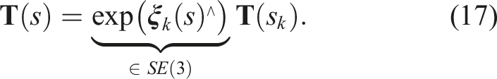
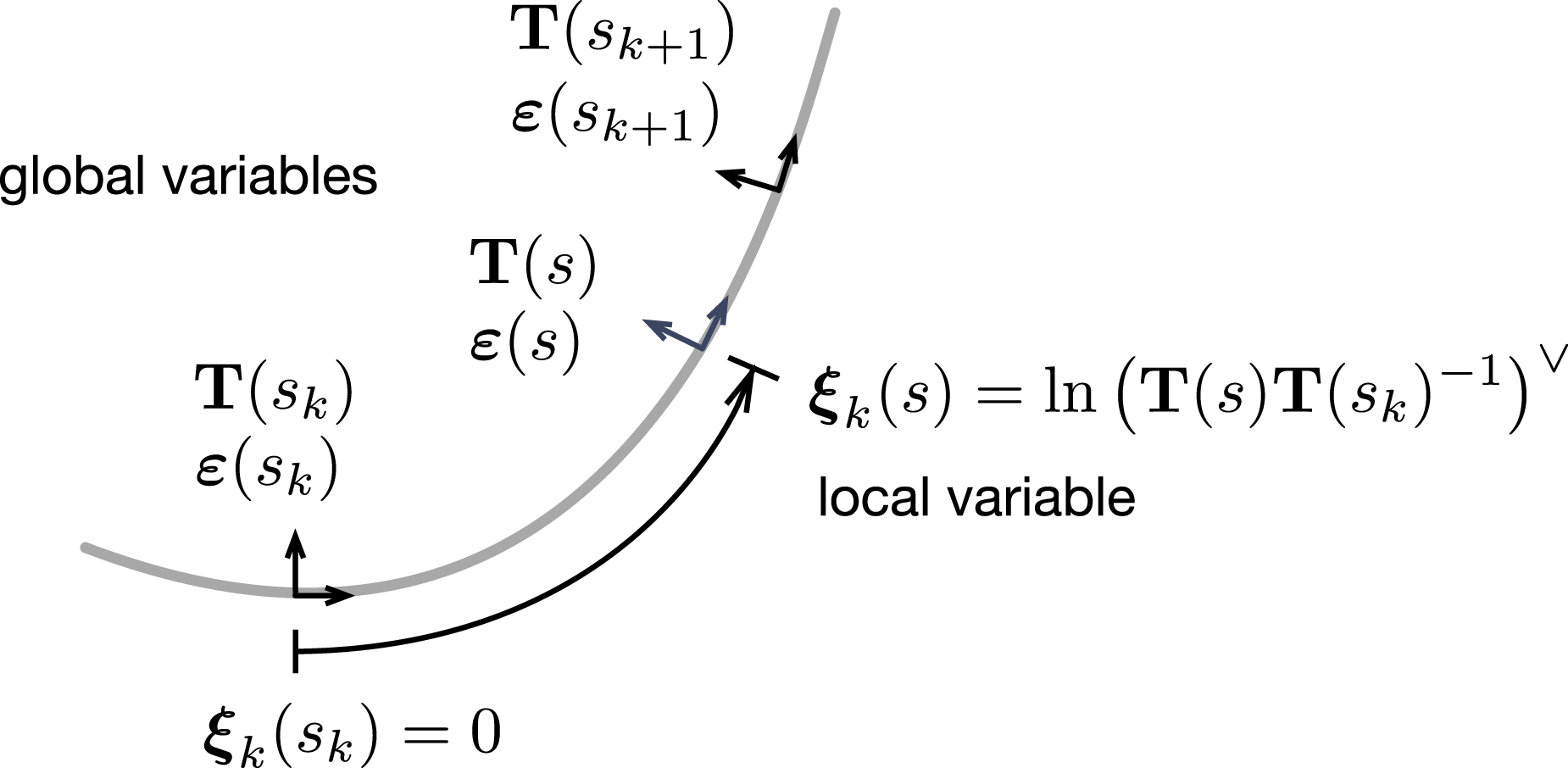
The local variable is essentially compounded onto its associated global pose. This allows us to convert back and forth between the global pose
We now choose to define our GP indirectly through a linear, arclength-invariant stochastic differential equation on the local variables (as opposed to the global ones)
In other words, we corrupt the second derivative of pose with a zero-mean, white-noise Gaussian process. We reorganize this into a first-order stochastic differential equation as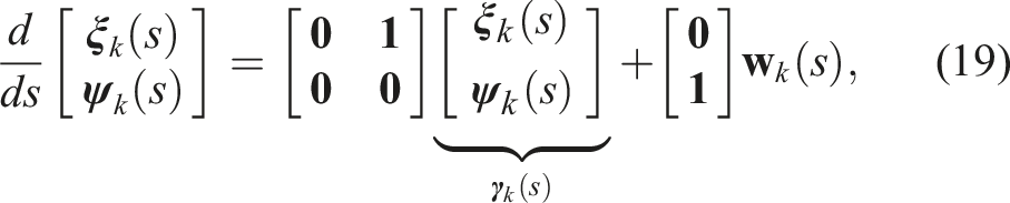
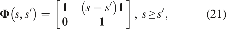
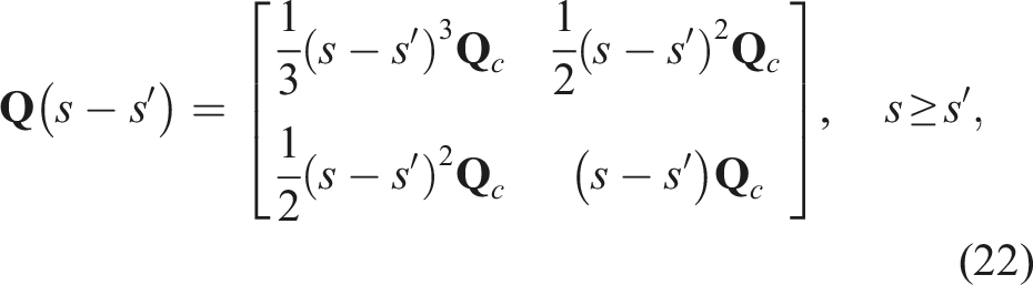
The local variable equation (19) is linear and stochastic integration can be done in closed form (Barfoot, 2017, §3.4); this was in fact the point of switching to the local variables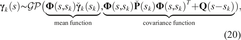
Our next goal is construct the overall cost function, whose minimizing solution will be the posterior distribution for the robot state. It will have two main terms, one for the prior and one for the measurements. We begin by constructing the prior term in this section and continue with the measurement term in the next. Normally in GP regression, we would build a kernel matrix between all pairs of unique states to be estimated (i.e., all pairs of arclength values whose state is to be estimated). However, because we have built our GP prior from a stochastic differential equation, it has an inherently sparse structure deriving from the Markovian property of the equation and we only need to evaluate the kernel between sequential states along the robot length (Barfoot et al., 2014). We define the error between two sequential values of the state as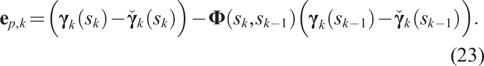
We can construct a cost term for this error as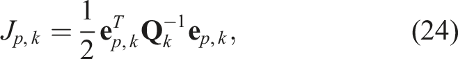
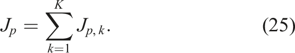
Figure 3 depicts the cost terms as a factor graph; each black dot represents one of the squared-error cost terms and the sum of these is our overall prior cost term. The prior for the entire robot state can be broken down into a sequence of binary factors (black dots), each of which represents a squared error term for how that pair of states is related. High cost is associated with shapes and strains that deviate from the prior mean (e.g., straight rod with no strain).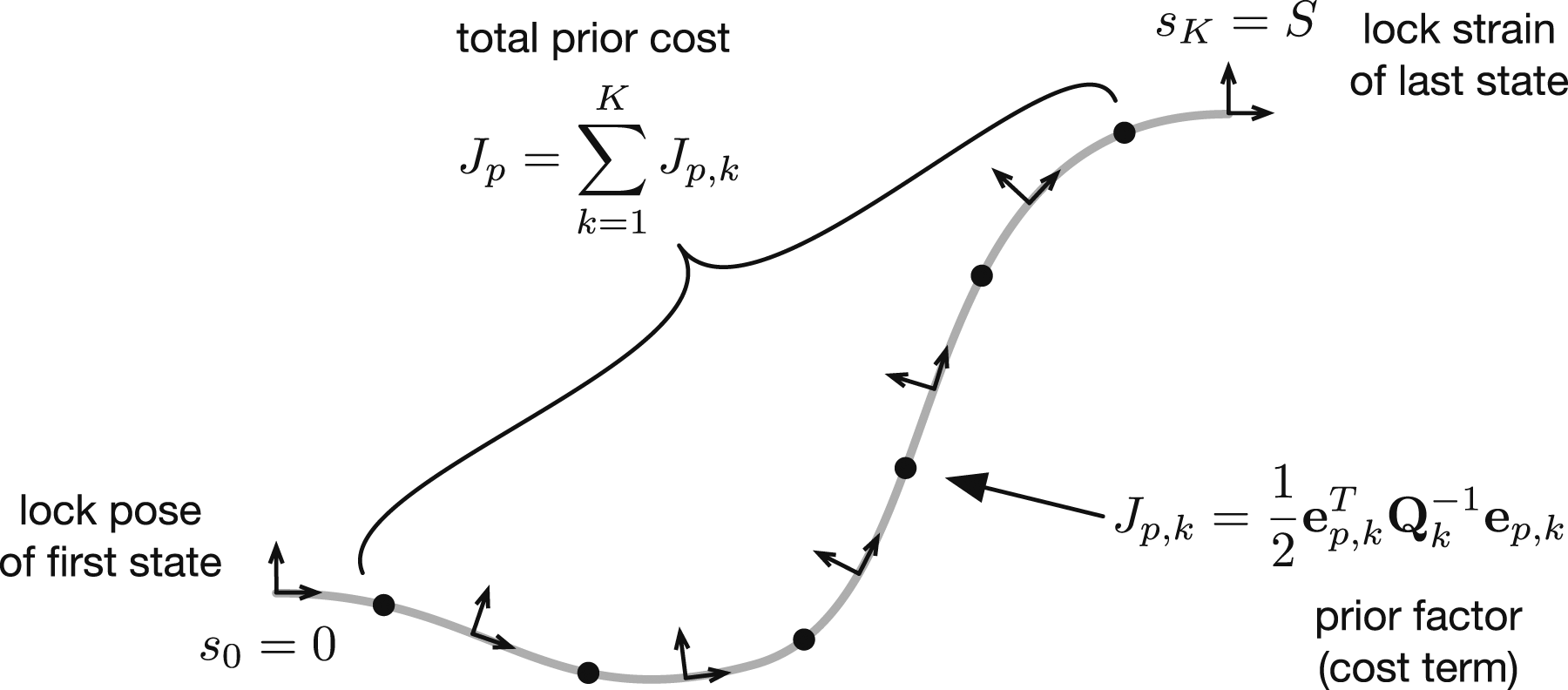
The last detail we need to work out is how to swap out the local variables in the error (23) for the original global variables since these are the ones we actually want to estimate. We can isolate for 
Another way to think about the development of the prior in this section is that we defined uncertainty affecting our state in the Lie algebra of the pose, where we could avoid the need to worry about the constraints on the variables. While this development is somewhat involved, the result is quite simple. We use (28) inside (24) to build a bunch of squared-error terms for the states at a number of discrete positions along the arclength of the robot, also known as factors as depicted in Figure 3. Figure 4 shows the mean function and 300 random samples drawn from the prior; we can see the prior allows for all kinds of quite different robot shapes. The hyperparameters of our prior are the nominal strain, Graphical depiction of the prior distribution over robot states. Here, we show the mean shape for the robot, a straight line along the x axis, as well as 300 random samples drawn from our GP prior. Here, we took S = 10, 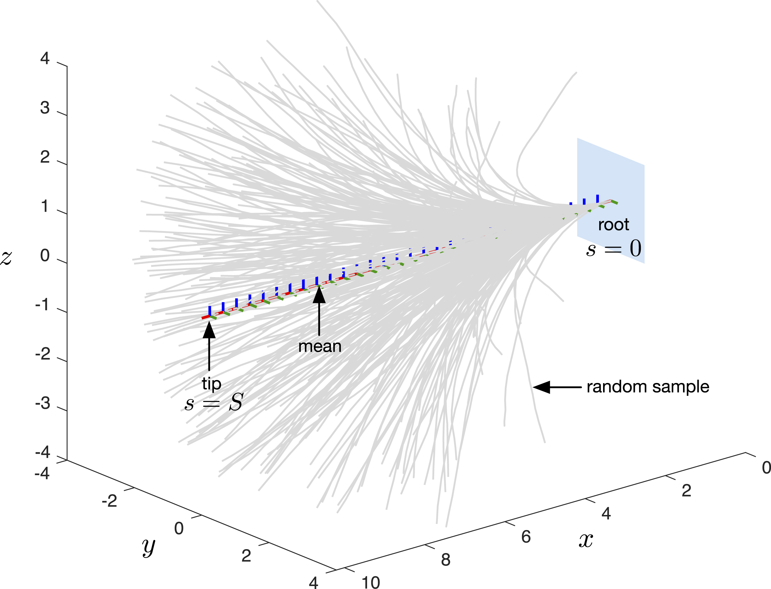
The next section will define similar squared-error terms for our measurements, and then we will then perform an optimization to find the best state for the robot as well as its associated uncertainty.
2.2.2 Measurements
Relatively speaking, the cost terms for the measurements are easier to explain than the prior from the previous section. We will consider two types of measurements corresponding to commonly used sensing modalities in continuum robotics: 1. Pose measurements: the pose (or part thereof) of a continuum robot can be measured at discrete arclengths either by an external camera system or magnetic coils attached to the robot. 2. Strain measurements: the strain (or part thereof) can also be measured at discrete arclengths using embedded strain gauges such as those employing fiber-optical Bragg gratings.
We consider that all measurements are noisy, and thus, we will probabilistically fuse our prior continuum robot model with these measurements to produce a posterior estimate of the shape and strain. Figure 5 depicts the measurements of pose and strain as unary factors, meaning squared-error terms involving the state at a single arclength. The next two subsections lay out the cost terms for the two types of measurements. The measurements (both pose and strain) make up unary factors (black dots), each of which represents a squared error term for how that state should be. High cost is associated with shapes and strains that deviate from the measurements. Here, we have a typical setup with a pose measurement of the end effector and two strain measurements at intermediate arclengths.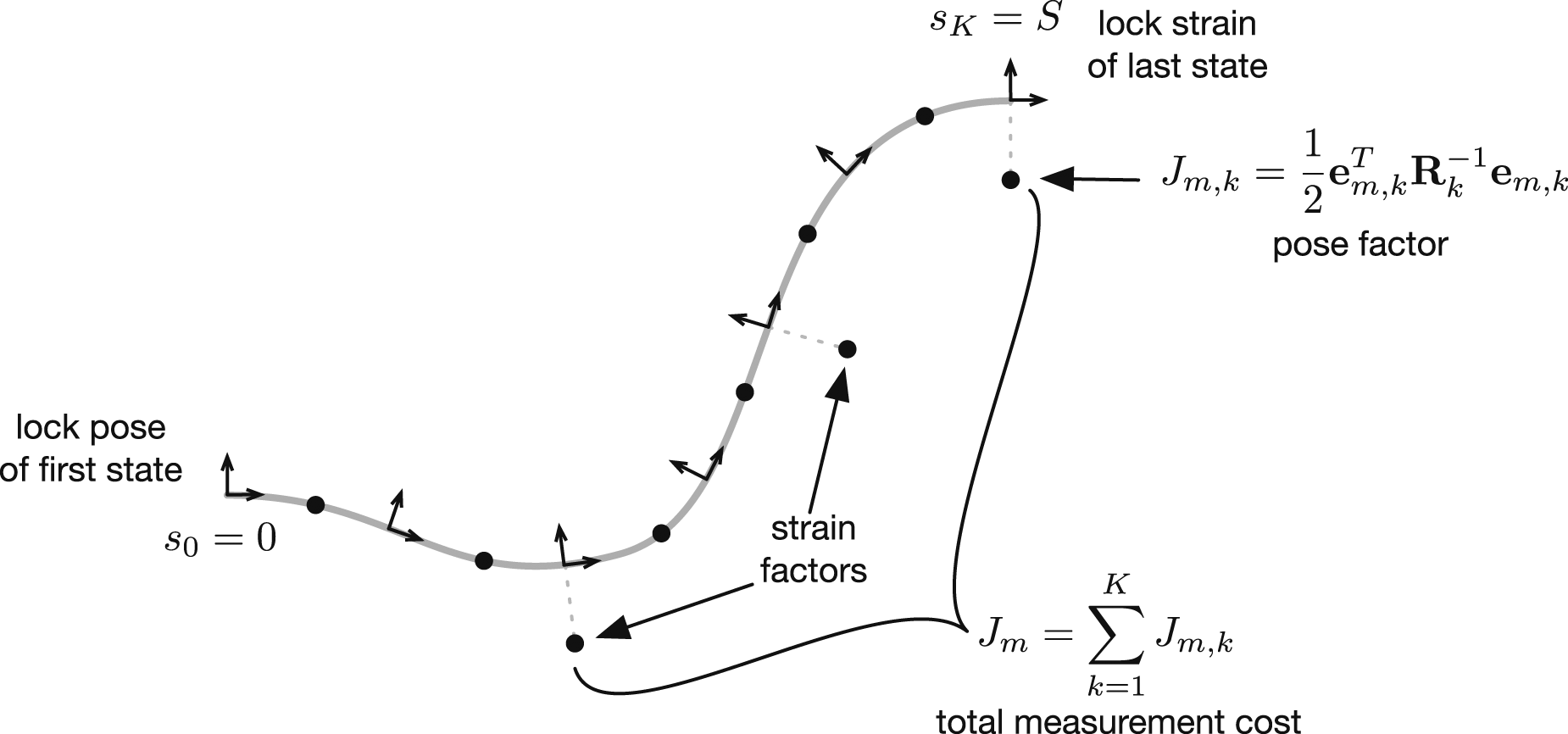
2.2.3 Pose measurements
Let us assume that the full pose of the robot state can be measured at a particular arclength, s
k
. Following Barfoot and Furgale (2014); Barfoot (2017), we assume this pose measurement, 
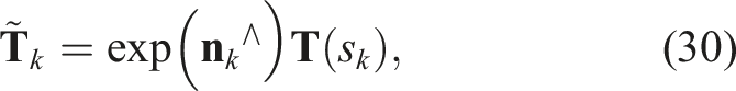
We can form an error for this pose measurement by reorganizing the measurement equation as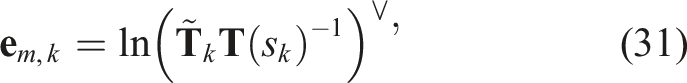
2.2.4 Strain measurements
Strain measurements are even simpler to handle than pose measurements as we do not need to contend with SE(3). We assume a measurement of the strain, 

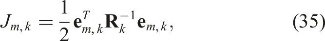
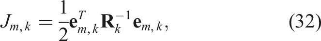
2.2.5 Optimization
Putting all of our cost terms together, the overall cost that we seek to minimize is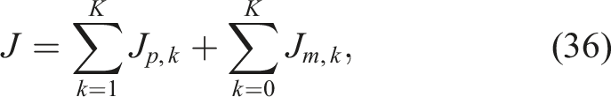
Our optimization problem is therefore
We use Gauss–Newton optimization to find our estimate, 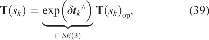

We can rewrite our cost function (36) using stacked quantities rather than summations as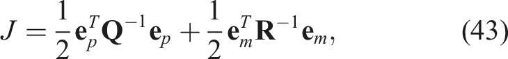
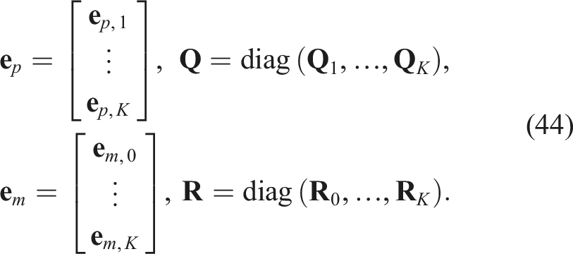
Inserting our perturbation schemes from (39) and (40), we can linearize the prior and measurement errors as
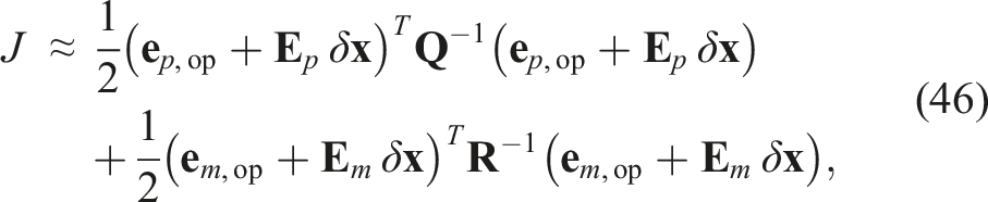
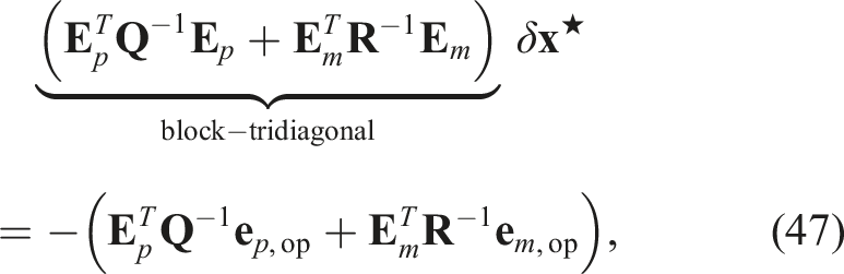


Figure 6 provides an example of the estimator in action. A single measurement of the end-effector pose is fused with the kinematics/physics prior. The caption provides further details. Example solution from our continuum robot state estimator with K = 30. A single noisy pose measurement of the end effector (located at (6, − 2, − 1) pointing down) is fused with the kinematics/physics prior. The left plot depicts the pose part of the state estimate including 3σ uncertainty ellipsoids for the position. The pose of the root is constrained to an identity transform and the strain of the tip is constrained to the nominal strain, 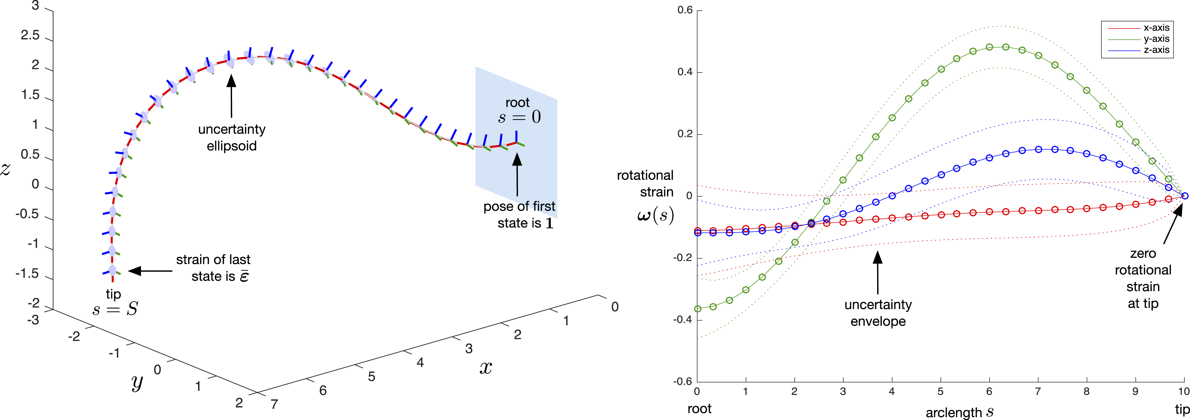
2.2.6 Error Jacobians
An outstanding item is to provide the details for the error Jacobians,
where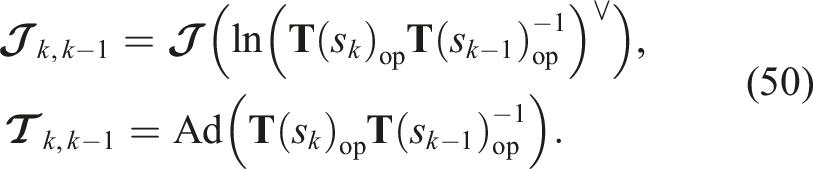
The blocks of
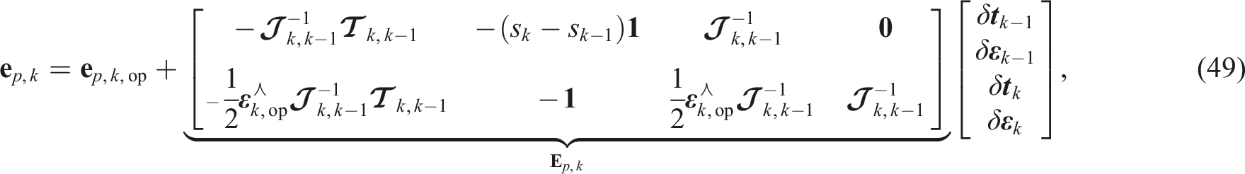
For the pose measurements, the error can be linearized as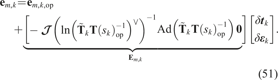
For the strain measurements, the error linearizes simply as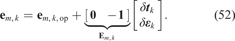
As with the prior terms, the blocks of
2.2.7 Extracting uncertainties
We have so far only discussed how to determine the most likely robot state in our optimization setup. To extract the uncertainties of the estimator (e.g., see Figure 6), we can turn to the common Laplace approximation, which fits a covariance at the most likely state. Naively, we could take the left-hand side of the linear system of equations (47) at the last iteration and invert this for the covariance, 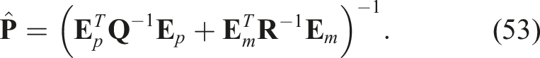
Although
It is worth mentioning how to interpret the 12 × 12 diagonal covariance block 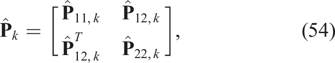


In other words, the uncertainty is expressed in the Lie algebra associated with the pose. Our marginal posterior estimate for the strain is simply
Another nice property of having set up the problem as a batch estimation is that we can in fact draw samples for the entire robot state from the full covariance in (53). Figure 7 shows an example where we have drawn 20 samples from the posterior and displayed them along with the mean. This is only possible if we have the full covariance since all the states are correlated with one another. Three viewpoints of an estimate with its mean (red-green-blue frames) and 20 samples drawn from the full Gaussian distribution (gray lines).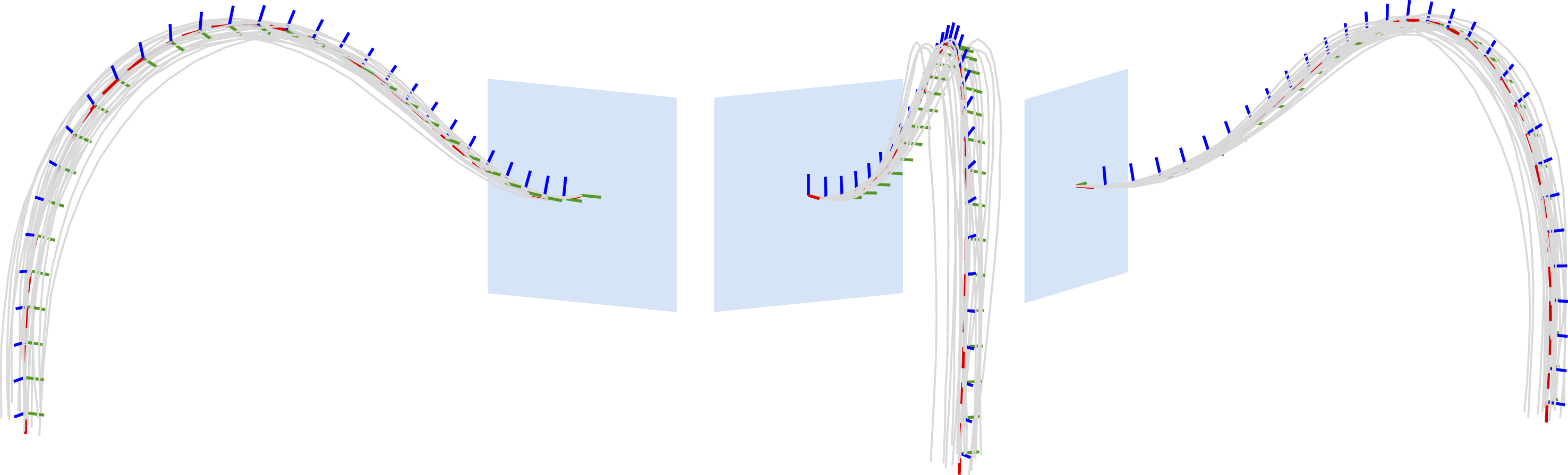
2.2.8 Querying the state between estimated arclengths
Because we have set up our problem using GP tools, we can easily use the built-in GP interpolation equations to query the mean and covariance of the state at any arclength of interest, including at arclengths not computed in the main optimization. For example, we might want to check how close our robot is to obstacles in a known environment, and we might therefore like to check the pose at a large number of arclengths (e.g., 10 times as many as were estimated) to be very confident a small object or corner does not come too close.
As shown by Barfoot et al. (2014); Anderson and Barfoot (2015); Barfoot (2017), we can perform a state (and covariance) query in O(1) time due to the special nature of our prior (i.e., that it came from a differential equation). If we want to make our solver as fast as possible, therefore, we would make the number of arclengths in the main solution, K, as small as possible and then query additional states after the fact. We omit the details in the interests of space but refer to Anderson and Barfoot (2015); Anderson (2016).
Figure 8 shows an example where we used only K = 10 for the original estimation problem and then queried 4 additional state values between each pair of estimated states. Importantly, we can see that the interpolation is not linear with respect to arclength but allows the robot to be curved. As discussed by Barfoot (2017, p. 86), the particular prior model that we chose (i.e., white noise on strain rate) results in cubic Hermite polynomial interpolation for the robot poses; however, this is a consequence of the prior selection and we can use the general GP interpolation equations without worrying about these details. One of appealing features of using the GP approach is the ability to query the state at any arclength of interest, after the main estimation has converged. In this example, we used K = 10 for the original estimation problem and then interpolated 4 extra state values between the estimated states. We can see that this interpolation is not linear but rather that it is based on the prior model we selected allowing it to be curved. Note, both the mean and the covariance can be queried in this way.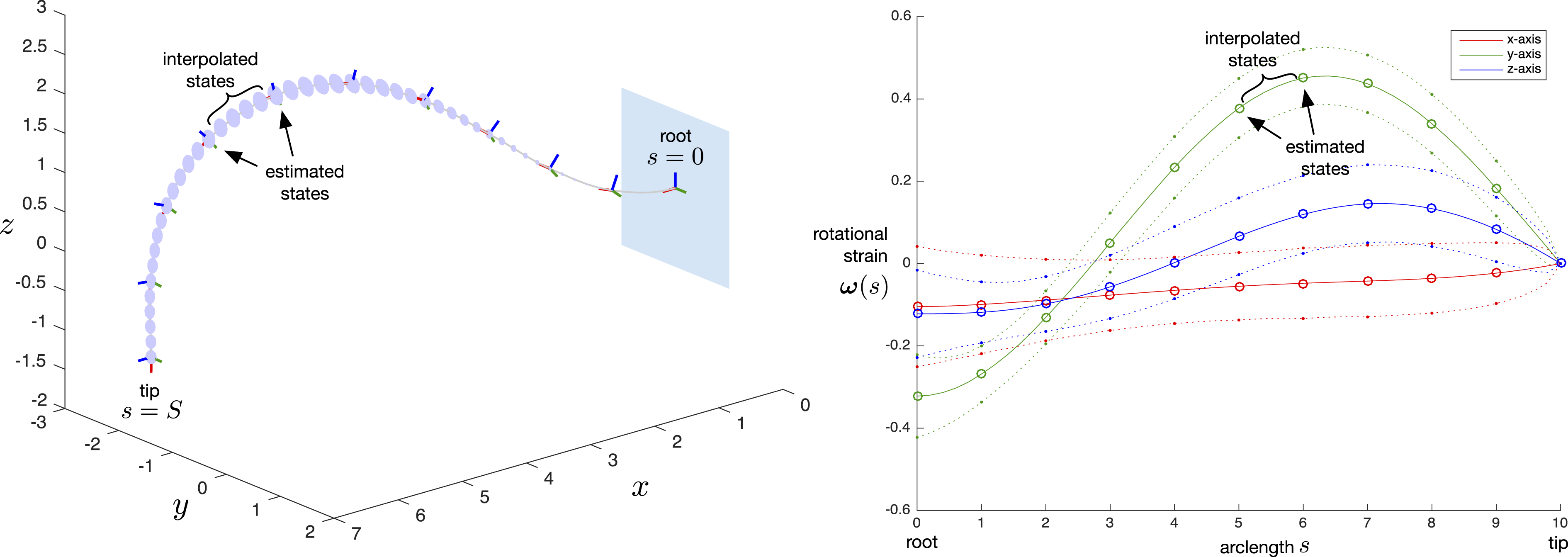
3 Evaluation
The state estimation approach proposed in this work is evaluated both in simulations and through experiments. While the proposed algorithm works for any structure or manipulator that can be accurately modeled using Cosserat theory of elastic rods, we focus on continuum robots actuated via tendons throughout this section as an example, which is one of the most commonly used and studied continuum robot types. This section first introduces the main principle of such so-called tendon-driven continuum robots. Afterward, experiments to evaluate the proposed approach in both simulations and on a real robotic prototype are described, before presenting and discussing the achieved results.
3.1 Tendon-driven continuum robots
Tendon actuation is one of the most commonly studied actuation principles for continuum robots to date. These so-called tendon-driven continuum robots (TDCRs) are realized by multiple tendons that are routed along their flexible backbone. The tendons terminate at predefined locations along the robot’s arclength, s. Thus, a TDCR can consist of multiple segments, with each segment end being defined by the termination of one of multiple tendons. Pulling and releasing these tendons applies a load to the compliant backbone, bending the corresponding segment in the direction of the routed tendon. Thus, the configuration
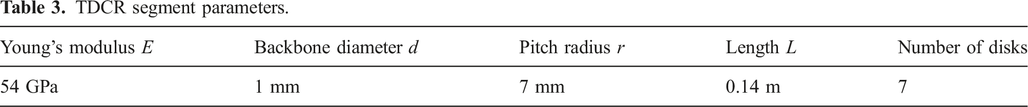
TDCR segment parameters.
3.2 Simulation
For simulation, a TDCR is simulated using the state-of-the-art Cosserat rod–based static model proposed by Rucker and Webster (2011). In particular, we are using a C++ implementation of that model published by Rao et al. (2021). An example rendering of the simulated two-segment TDCR is shown in Figure 9 (left). Left: Example rendering of a simulated tendon-driven continuum robot consisting of two bending segments. Right: Overview of 100 random samples of the simulated TDCR. Half of the samples are unloaded configurations, meaning that the deformation of the robot solely resulted from pulling different tendons (light gray), while the other half includes a randomly generated wrench acting at the tip of the robot (dark gray).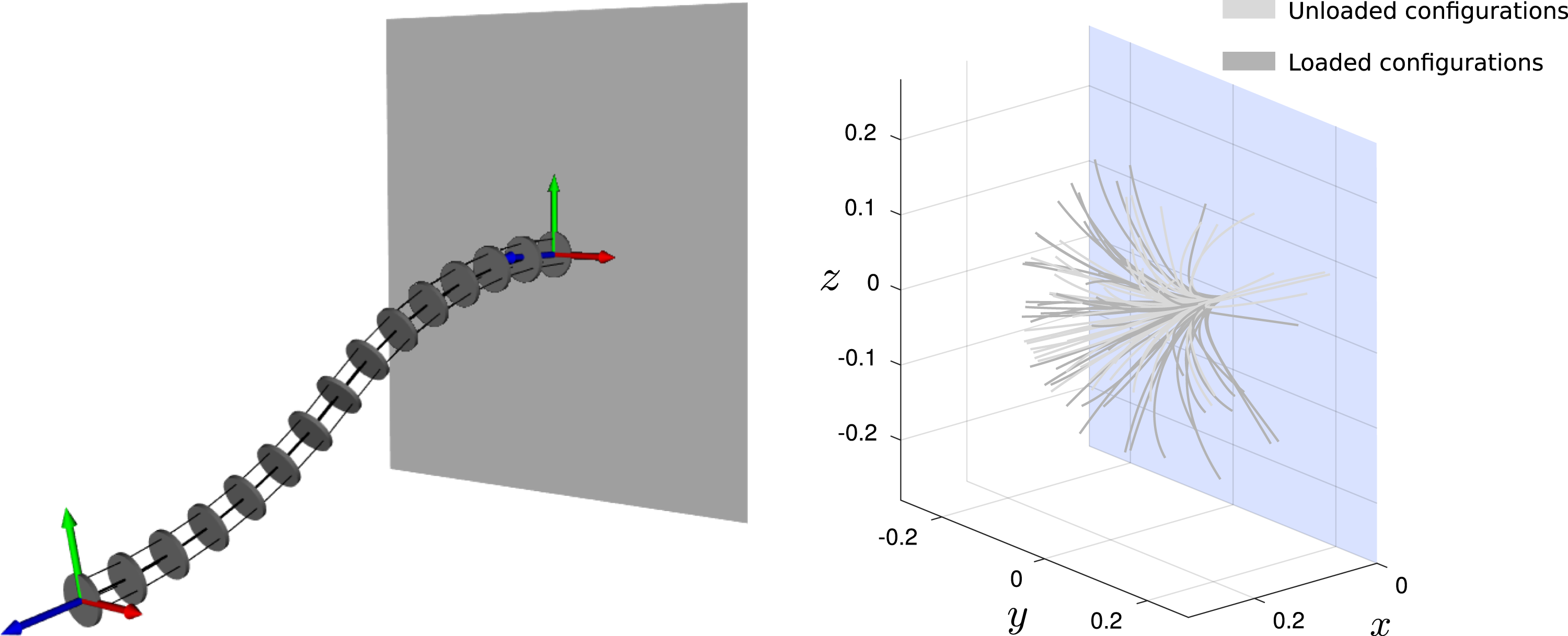
3.2.1 Data set generation
Using the simulated TDCR, a data set consisting of 100 different robot configurations is sampled. This is done by drawing random samples from the valid joint space of the robot and using the forward kinematics to obtain the resulting robot state. Specifically, we consider tendon forces of up to 3N, so that each randomly sampled joint value is
3.2.2 Creating noisy sensor data
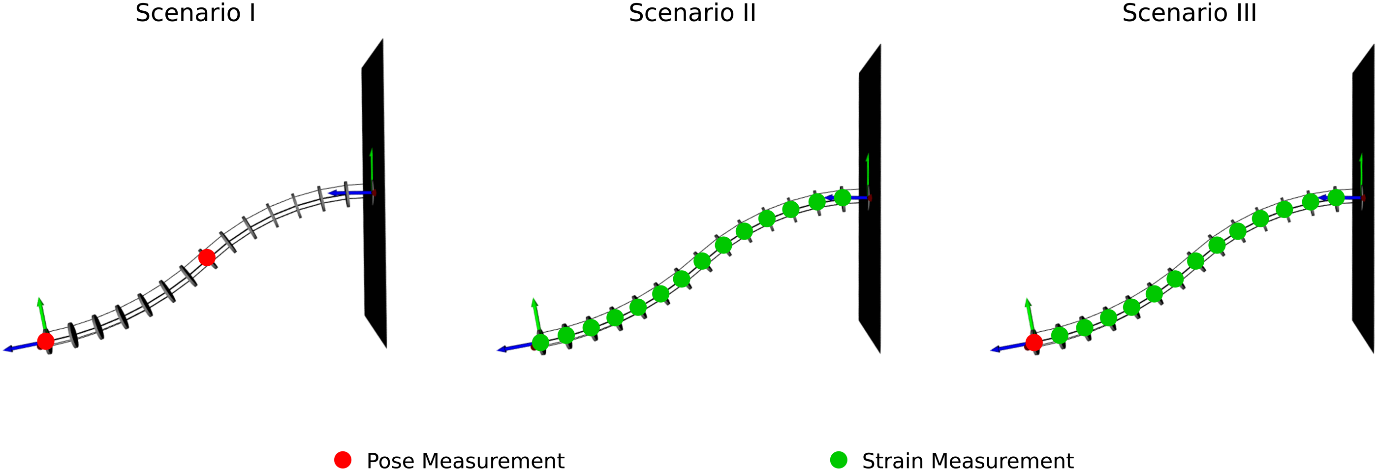
In the next step, noisy sensor measurements are simulated using the ground truth data set. We consider three different scenarios for possible sensor placements (see Figure 10), each of which are commonly used and proposed for continuum robots: 1. Pose measurements at the end of each robot segment (i.e., at its tip and at half of its length). 2. Multiple discrete strain measurements at each of the robot’s disks’ location. 3. Multiple discrete strain measurements in combination with a single pose measurement at the robot’s tip. To evaluate the state estimation algorithm proposed in this work, three different sensor placement scenarios are considered: pose measurements at the end of each robot segment (left), discrete strain measurements at each robot disk (middle), discrete strain measurements at each disk in combination with a single pose measurement at the robot’s tip (right).
Both pose and strain information are relatively common when sensing the state of a continuum robot. For instance, an accurate pose measurement can be obtained using electromagnetic tracking coils (Mahoney et al., 2016), while strain measurements can be enabled using fiber Bragg gratings (Shi et al., 2017).
We simulate the sensor measurements by extracting the pose and strain values at the corresponding arclengths from our simulated ground truth data set. Afterward, we inject noise on each of the components of the simulated measurements. This is done by drawing random values from a zero-mean normal distribution, where standard deviation is the noise variable. These noise variables are chosen in a way to mimic realistic conditions and errors of the particular sensors that would be used to obtain these measurements. In particular, we chose the standard deviations for the position and orientation of the pose as σ
t
= 1 mm and σ
a
= 0.01 rad, respectively. The standard deviations for both the translational and rotational strain are set to σ
ν
= σ
ω
= 0.05. While for the strain variables, the noise can simply be added to the vector itself, we inject the noise to the pose in an
3.2.3 Hyperparameter tuning
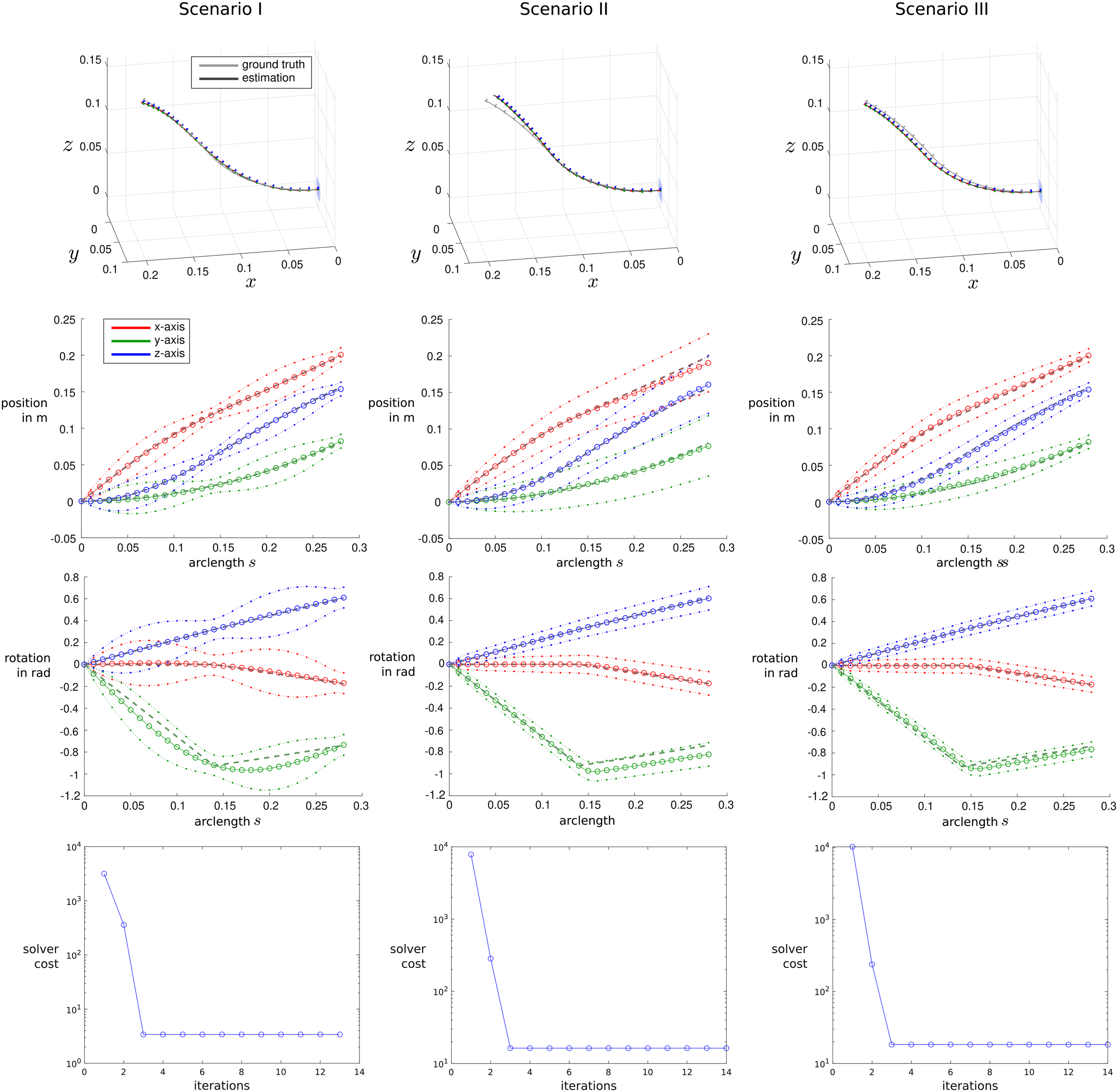
All hyperparameters were tuned empirically using a typical TDCR configuration (see Figures 11 and 12) and considering all of the three sensor placement scenarios stated above. The covariance matrices for the pose and strain measurements are set as Example TDCR configuration, in which the deformation is mainly dominated by bending around the y-axis. The plots on the left show the y-component of the robot’s orientation (expressed as an angle-axis pair) as well as the y-component of the rotational strain along its arclength s. Each plot shows the mean along with the 3σ uncertainty envelopes and the simulated ground truth (dashed line). Results from the proposed state estimation algorithm using a typical TDCR configuration. Three different sensor placement scenarios are considered: Pose measurements at the end of each robot segment (left), discrete strain measurements at each robot disk (middle), and discrete strain measurements at each disk in combination with a single pose measurement at the robot’s tip (right). The resulting continuous estimated shapes are plotted using colored frames on the left with ground truth shapes plotted in gray. Additional plots display the x- (red), y- (green) and z-components (blue) of the robot’s translation and orientation (expressed as angle-axis pair) along its arclength s. The plots show the mean along with the 3σ uncertainty envelopes and the simulated ground truth data (dashed line). The bottom plots show the cost of the optimization problem over the number of iterations.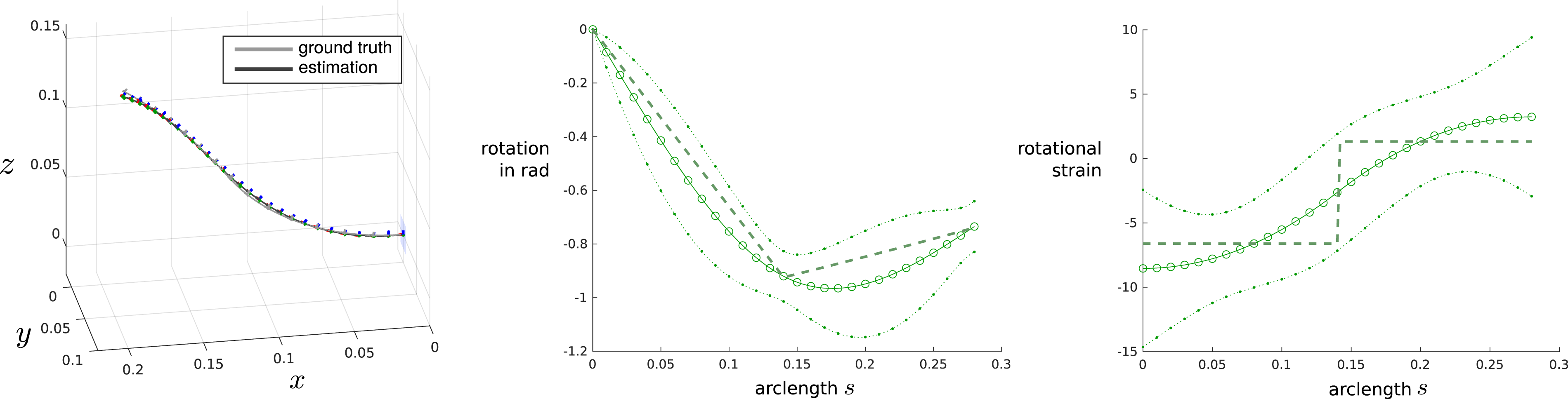
We note that with the current choice of covariance matrices, we put relatively high trust into the measurements, while the prior cost is weighted relatively low in the optimization problem. This way, the prior is mainly used for smoothing the solution of the regression problem, while sufficient sensor information is present to provide a good estimate about the resulting state and shape of the robot.
We further note that tuning the hyperparameters is a non-trivial procedure as it depends on a number of different factors including the robot type, the type and number of sensors as well as the covariance and resulting confidence of these sensor readings. While we chose to manually tune the hyperparameters in order to obtain desirable state estimates for the two-segment TDCR prototype in different sensor placement scenarios, future work should investigate more sophisticated optimization routines to identify these hyperparameters by using a larger set of calibration data. For example, one could follow the approach proposed by Wong et al. (2020), in which the parameters in a Gaussian variational inference setting are learned to obtain accurate state estimates of vehicle trajectories.
While tuning the hyperparameters for our TDCR design, we observed the resulting strain profiles of the simulated ground truth data. Due to the nature and design of TDCR, the actuation loads that are acting on the robot are dominated by moments acting at discrete positions along the arclength at which the tendons of a segment terminate. This results in a loading profile that is highly discontinuous, which also leads to a highly discontinuous strain profile with large jumps at the end of each respective TDCR segment. An example of this is shown in Figure 11, which features a TDCR configuration that is mainly dominated by bending deformations around the local y-axis. Both the y-component of the robot’s orientation (represented as an angle-axis pair) and the y-component of the rotational strain are plotted along the arclength s. It can be seen that the rotational strain is approximately constant for each individual bending segment. It remains constant until the distal arclength s = S, where theoretically another discontinuity occurs, at which the strain jumps to zero. When not locking the strain variables at s = S, the resulting estimated strain variable profile generally matches the simulated discontinuous one more closely, which results in slightly more accurate state estimates. Thus, we did not lock the strain variables at s = S during simulations and experiments in the following. However, we note that locking the strain at the tip of the rod is still the theoretically correct and widely used boundary condition for continuum robots.
3.2.4 Results
Detailed state estimation results for the configuration used to tune the hyperparameters are shown in Figure 12. The estimated and ground truth robot shapes are plotted on the left, while the individual estimated and ground truth position and orientation components together with the 3σ uncertainty envelopes are plotted on the right. The three different sensor placement scenarios discussed above are considered, where the plots on the top consider two pose measurements at the end of each robot segment, the plots on the middle consider discrete strain measurements at each disk, and the plots on the bottom consider strain measurements with a single pose measurement at the robot’s tip. It can be seen that in each of the three scenarios, the robot shape can accurately be estimated. Larger deviations occur when only strain measurements are considered, which is to be expected as small errors and uncertainties are integrated along the arclength of the robot and can easily accumulate. However, the ground truth remains close to the estimated shape and lies within the plotted uncertainty envelopes. As expected, these envelopes are tighter when the estimation is more confident, which usually is the case, when an accurate measurement is present. This behavior can most notably be observed in scenarios with pose measurements, in which both the envelopes for position and orientation tighten around the discrete measurements. In the top plots, the envelops tighten at the end of each segment, while they only tighten at the tip of the robot in the bottom plots. When considering only strain measurements, the uncertainty of the estimation increases along the robot’s arclength, as expected. Throughout all of the three different sensor placement scenarios, convergence of the optimization routine occurred after three iterations, as indicated by the cost term plots at the bottom of Figure 12. Based on these results and the sparsity of the resulting linear system of equations, we anticipate that our proposed method can be utilized in real-time applications.
For a more general evaluation, we run the state estimation approach for each of the 100 configurations included in our data set, while considering the previously described sensor placement scenarios. For each run, we calculate both the position and orientation errors of the state estimation approach with respect to the simulated ground truth data along arclength s, considering M = 5 interpolated states between the K nodes. The position and orientation errors averaged over all configurations of our data set are plotted in Figure 13. Again, we are considering the three sensor placement scenarios previously discussed: two discrete pose measurements, multiple discrete strain measurements, and a single pose measurement at the tip in combination with the strain measurements. Position and orientation errors of the interpolated estimated state with respect to the simulated ground truth data along arclength s considering all of the 100 simulated TDCR configurations from the sampled data set. The mean errors are shown in black, with the standard deviation plotted with dashed lines. The red and blue graphs show the maximum and minimum occurred errors at the corresponding arclength s. Three different sensor placement scenarios are considered: Pose measurements at the end of each robot segment (left), discrete strain measurements at each robot disk (middle), and discrete strain measurements at each disk in combination with a single pose measurement at the robot’s tip (right).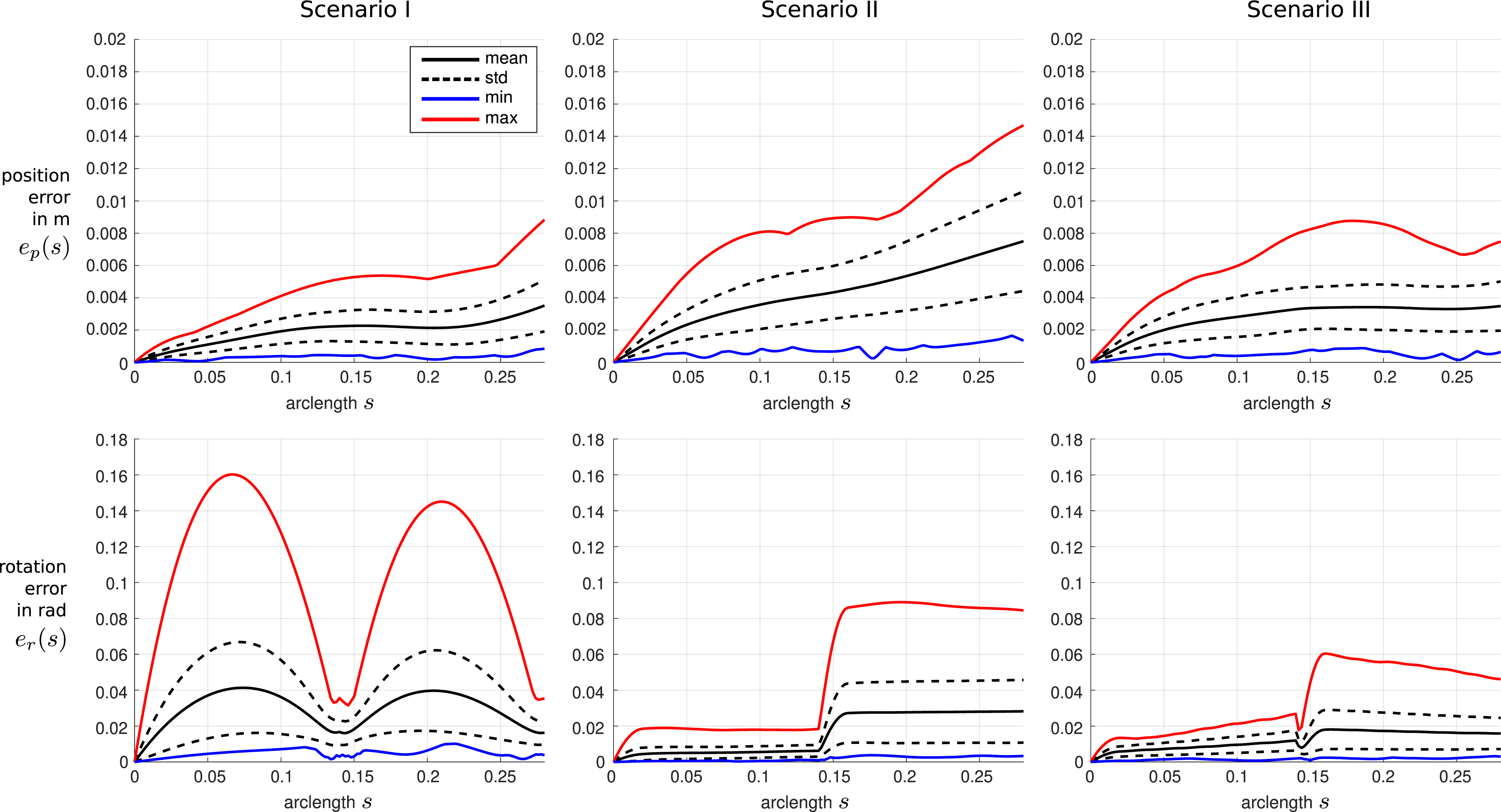
It can be seen that overall, relatively low errors between the shape estimation and the ground truth data occur. Larger errors occur when only considering strain measurements, while pose measurements help to reduce the error significantly at the specific arclength positions. In comparison to the results with strain measurements only, where the position error increases with respect to the robot arclength, pose measurements help to bound the error. Overall, the average errors at the tip of the robot over all 100 configurations result in 3.5 mm and 0.016° for the pose measurement scenario, 7.5 mm and 0.028° for the strain measurement scenario, and 3.5 mm and 0.016° for the pose and strain measurement scenario. We do note that there will always be some error between the estimation and ground truth since noisy sensor data is used in the estimation algorithm.
3.3 Experiments
The proposed algorithm is further evaluated using real robot experiments. In order to do so, a two-segment TDCR prototype is built using the parameters stated in Table 3. The prototype consists of a super-elastic nitinol backbone and spacer disks, that are used to route four tendons per segment along the robot’s backbone. The spacer disks are fabricated using a stereolithography resin 3D printer (Form 3, Formlabs Inc., USA). The robot can be actuated by pulling different combinations of those tendons. The prototype is shown in Figure 14 on the left. Experimental setup including the TDCR prototype and the electromagnetic tracking system (left); laser scan of the TDCR prototype with spheres extracted from the point cloud to reconstruct the frame of each disk (middle); extracted colored ground truth frames of each disk from the laser scan together with two gray disk frames measured by the electromagnetic tracking system (right).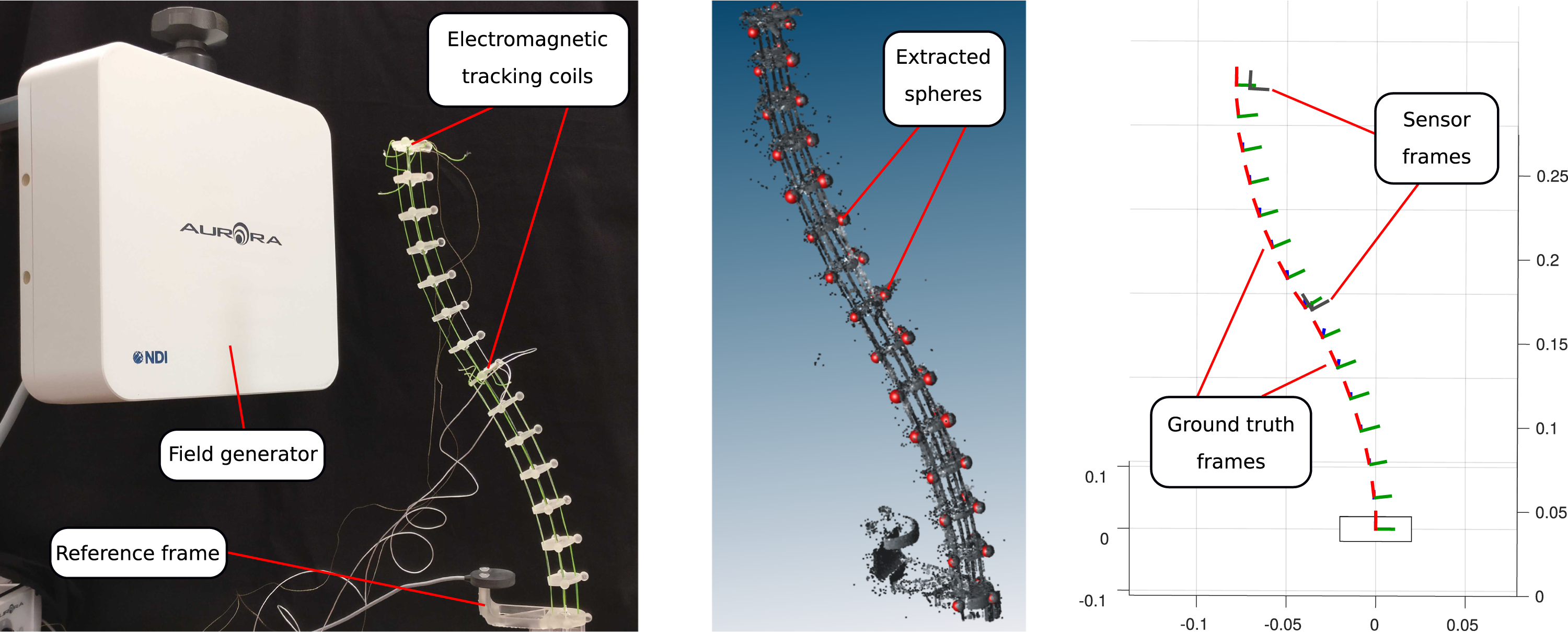
3.3.1 Sensor setup
For the experimental evaluation, we consider the sensor placement scenario with two discrete pose measurements, one at the end of each robot segment. In order to obtain these pose measurements, an electromagnetic tracking system (Aurora v3, Northern Digital Inc., Canada) is used. Two custom 6-degree-of-freedom tracking coils are rigidly attached to the spacer disks at the end of the corresponding robot segment. A third tracking sensor is attached to the base of the robot to serve as 6-degree-of-freedom reference frame. Using its measured position and orientation data and the known transformation between the sensor mounting point and the base of the robot, the transformation between the electromagnetic tracking system and the robot’s base frame can be calculated. The used tracking sensors have a stated root mean square error of 0.8 mm and 0.7° by the manufacturer.
In addition to the sensor readings from the electromagnetic tracking system, the shape of the robot is reconstructed using a highly accurate external laser scan. This data serves as ground truth in order to assess the accuracy of the proposed state estimation algorithm. The shape is represented as a frame of each of the robot’s disks. The robot is scanned using a coordinate measurement arm with attached laser probe (FARO Edge with FARO Laser Line Probe HD, FARO Technologies Inc., USA). The laser probe allows to obtain accurate point cloud readings of the robot’s shape. Each printed disk holds three spheres with diameters of 5 mm, that can be easily identified and extracted from the corresponding point cloud. Using the position of these three spheres and the disk’s known geometry, the frame holding the spatial position and orientation can be reconstructed for each. On top of that, the robot’s base also contains three spheres, to identify its frame. Thus, the transformation between the measurement arm system and the robot’s base frame can be computed.
The experimental setup as well as the extraction of ground truth and sensor frame is shown in Figure 14. Finally, both the electromagnetic sensor readings and the point cloud extractions can both be represented with respect to the robot’s base frame, allowing it to use them in the state estimation algorithm and compare them with respect to each other. However, the calibration between the two distinct measurement systems might be slightly inaccurate for multiple reasons. First, errors might occur in the calculated transformation between the electromagnetic sensing system and the robot’s base frame arising from uncertainties in sensor placement and inaccuracies in the 3D printed base frame. Second, the accuracy of the transformation calculated for the ground truth data obtained from laser scans highly depends on the accuracy of the sphere extraction. In order to overcome these inaccuracies and to better align the two measurement systems, an optimization based calibration routine is employed in the later sections.
3.3.2 Data collection
Nine different TDCR configurations are used for the experimental validation. These configurations are obtained by actuating different combinations of tendons of the continuum robot, leading to different shapes covering different areas of the robot’s workspace. For each of these configurations, the two pose measurements from the electromagnetic sensors at the end of each segment are recorded. In addition, the ground truth disk frames are extracted using a laser scan. The resulting robot shapes for each configuration are plotted in Figure 15 (left). In the following, three out of these nine configurations are used to further calibrate the transformation between the individual sensing systems and the robot base frame. These three configurations are shown in gray in the plot. The remaining six configurations are then used to evaluate the proposed state estimation approach. Left: Shapes of nine TDCR configurations considered for the experimental validation of the state estimation approach. Three configurations (gray) were used to calibrate the sensing system to the ground truth data obtained from the laser scan, while the remaining six configurations (colored) are used to assess the performance of the shape estimation algorithm. Right: Shapes of three loaded TDCR configurations (colored), resulting from applying a tip load to a TDCR configuration in different directions. The initial unloaded configuration is plotted in gray and the directions of the applied loads are shown in orange.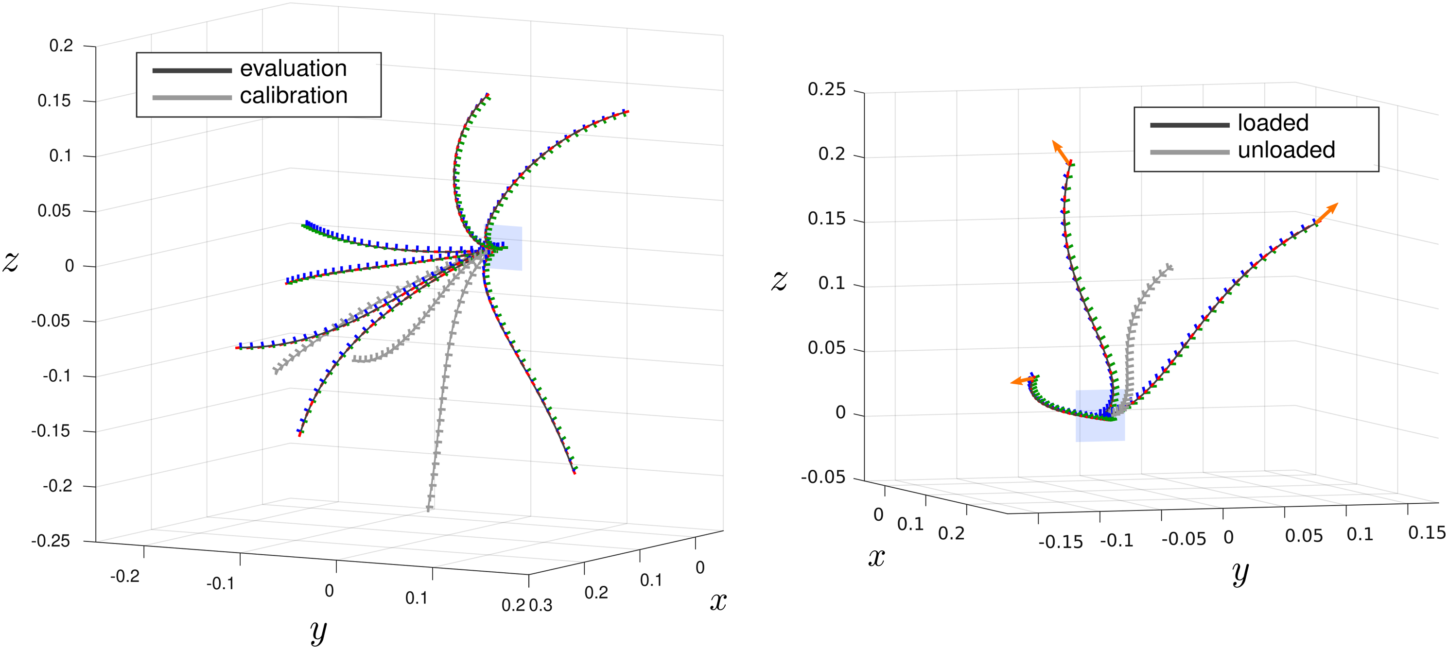
For further evaluation of our proposed method, we are also considering three TDCR configurations, in which an additional force of approximately 0.2 N is applied to the robots tip. The resulting robot shapes for these configurations are plotted in Figure 15 (right). The initial, unloaded TDCR configuration is plotted in gray, while the shapes of the three loaded configurations are colored. The directions of the applied tip forces are plotted in orange.
We note that the number of evaluation configurations is relatively low, mainly due to the time-consuming manual process of extracting the ground truth shape and frames from the laser scan.
3.3.3 Calibration
As stated above, we aim to further calibrate the alignment of the two individual measurement systems used throughout the experimental evaluation. We achieve this by employing a numerical optimization scheme using three of the nine recorded unloaded TDCR configurations. In particular, we aim to minimize the offsets between the ground truth frames and the frames obtained from the electromagnetic sensors for the two disks at the end of the robot’s segments. Thus, we have two data points per configuration, totaling in six data points for this optimization problem. We want to find the transformation matrix between the measurement arm laser probe base frame and the base frame of the electromagnetic tracking system that minimizes the average position error between the two measurement systems for the six data points. We implement a simple numerical optimization routine in
3.3.4 Results
The state estimation algorithm was run on the remaining six configurations of the TDCR prototype. The hyperparameters remained the same as tuned in Section 3.2.3 to remain comparable to the results obtained in simulation. The only exception is the number of interpolated states, which was changed to M = 2. We run the state estimation approach for each of the six TDCR configurations, while considering the previously described sensor placement scenario, in which the pose of the end and middle disk of the robot are measured using electromagnetic tracking sensors.
Detailed state estimation results for three example configurations are shown in Figure 16, one of which has a force applied to its tip (bottom). The estimated and ground truth robot shapes are plotted on the left, while the individual estimated and ground truth position and orientation components together with the 3σ uncertainty envelopes are plotted on the right. Agreeing with the results from simulations, the robot shape can accurately be estimated. The ground truth measurements remain close to the estimated shape and lies within the plotted uncertainty envelopes. Again, these envelopes are tighter when the estimation is more confident, which usually is the case, when an accurate measurement is present. Example results from the proposed state estimation algorithm using three of the evaluated configuration of the TDCR prototype—the top two configurations are unloaded, while the bottom configuration has an additional force applied to its tip. The resulting continuous estimated shapes are plotted using colored frames on the left with ground truth frames plotted in gray. The plots on the right display the x- (red), y- (green), and z-components (blue) of the robot’s translation and orientation (expressed as angle-axis pair) along its arclength s. The plots show the mean along with the 3σ uncertainty envelopes and the ground truth data from the laser scans (cross marks).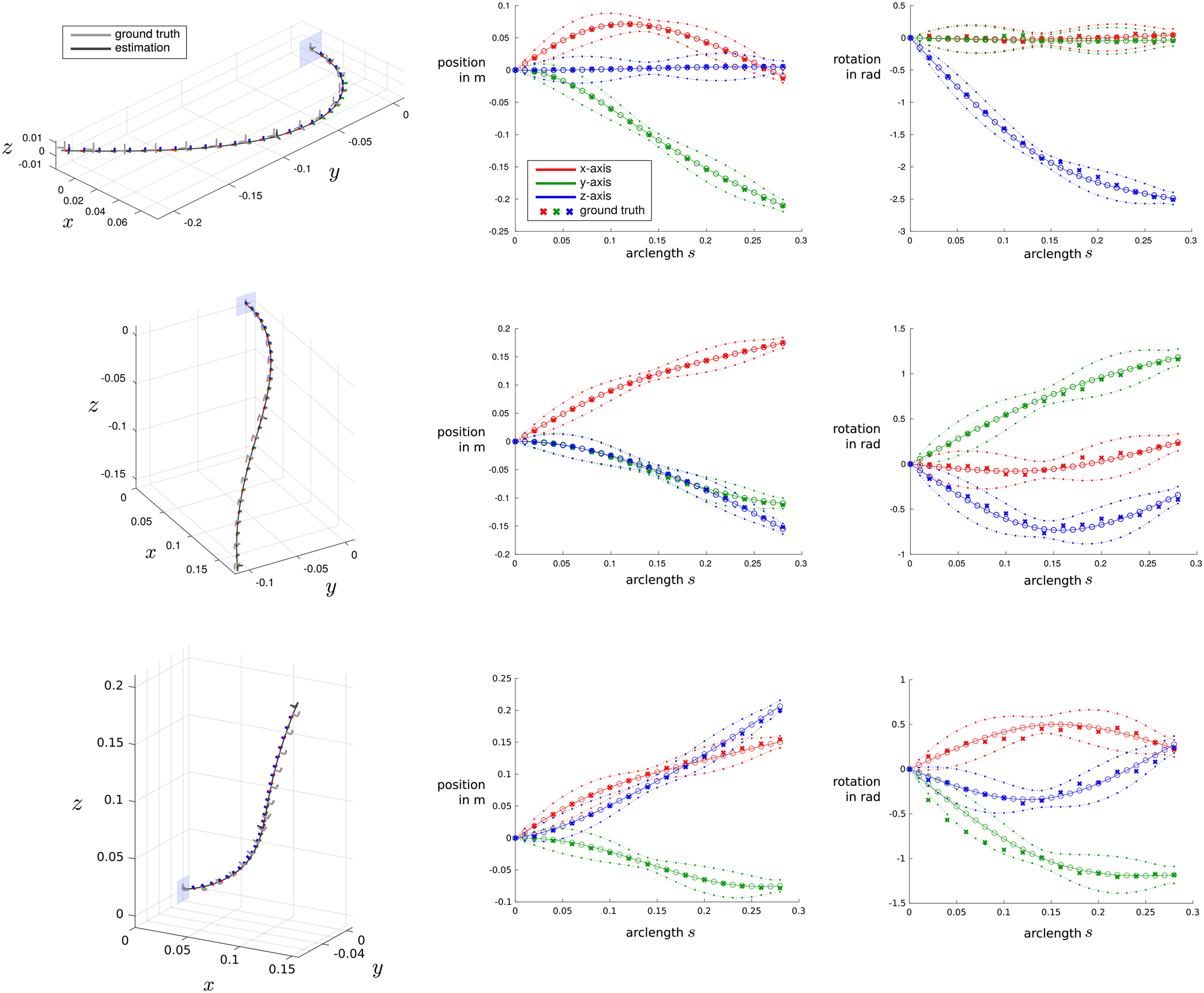
The position and orientation errors averaged over all of the six unloaded and three loaded TDCR configurations are shown in Figure 17. It can be seen that overall, relatively low errors between the shape estimation and the ground truth data occur. Specifically, average end-effector errors of 3.3 mm and 0.035° are achieved for the unloaded configurations. For the loaded configurations, the average end-effector errors result in 6.2 mm and 0.041°. These errors and their overall trend agree very well with the results seen in simulation. However, orientation of the estimated shape appears to be less accurate than the position when compared to the ground truth, as larger deviations are present. We note that the orientation of the reconstructed ground truth disk frames from the laser scan might be slightly inaccurate due to slight misalignments between the disks and the backbone during manufacturing as well as inaccuracies during sphere extraction. Thus, the errors might not be solely attributed to the state estimation algorithm. Position and orientation errors of the estimated state with respect to the ground truth data obtained from the laser scan along arclength s. Top: Six unloaded TDCR configurations are plotted in gray, while the mean errors across all six configurations are shown in black. Bottom: Three TDCR configurations with an additional tip load are plotted in gray, while the mean errors across all six configurations are shown in black.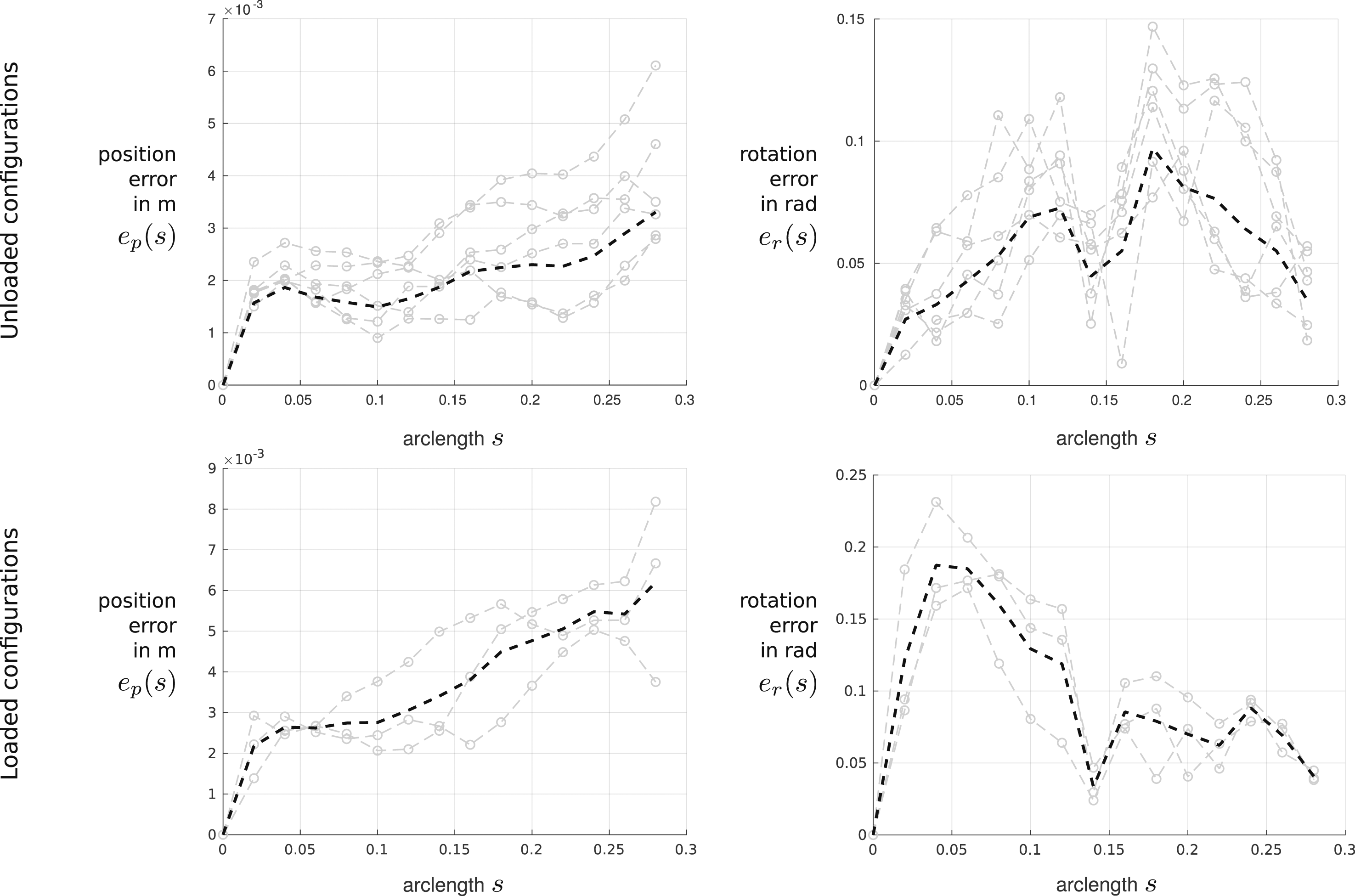
4 Discussion
The results presented in the previous section indicate that accurate shape estimates based on limited sensor information can be achieved by the proposed state estimation approach, resulting in average position and orientation errors at the end effector as low as 3.5 mm and 0.016° in simulation or 3.3 mm and 0.035° for unloaded configurations and 6.2 mm and 0.041° for loaded ones during experiments, when using discrete pose measurements. The evaluation carried out in this work is limited to a multisegment TDCR. However, the general formulation of the utilized Cosserat rod model makes the method applicable to a large variety of continuum robots. The main advantages of the proposed approach include the continuous estimation of the robot’s state, allowing for easy interpolation between nodes (mean and covariance), as well as the sparse formulation of the GP regression, requiring little computational effort.
We note that the current formulation of the prior will always lead to continuous profiles for the continuum robot’s estimated state, including both pose and internal strains along the arclength s. However, the presence of a discrete point load acting on the robot structure at a particular location along s can in fact lead to a discontinuous strain profile. One example of this can be seen in the multisegment TDCR considered in this work. The tendons routed along the robot’s structure apply discrete bending moments at their termination location, leading to a sudden and discontinuous change of the internal bending strain. In such cases, the state estimation approach will fit a smooth and continuous strain profile, which will differ from the ground truth and can lead to inaccuracies in the estimation. An example of this can be seen in the simulation results using strain measurements presented in Figure 13. In this case, the orientation error increases significantly at the end of the first segment, which is located at half of the robot’s total length.
Further, we would like to point out that the approach presented in this work is a local optimization method and therefore heavily depends on the chosen initial guess. A poorly chosen initial guess, which is far away from the robot’s ground truth and the corresponding sensor measurements, can lead to convergence to a local minima, that does not necessarily align with the expected robot shape. This problem could be overcome by using a more informed initial guess than the initially straight shape that is used throughout this paper. This initial guess could for instance be obtained from a kinetostatic model, relating known robot actuation inputs to a resulting robot shape. An example of this is shown in Figure 18 for a two-segment TDCR. In this example, the ground truth shape of the robot results from tendon actuation with an additional external force at the robot’s tip and is highly curved. Two pose measurements, one at the end of each robot segment, are used to estimate the robot’s shape with the approach proposed in this paper. Using a straight shape as an initial guess (top) results in convergence to a local minima, that aligns with the sensor readings but not with the expected ground truth shape. Using the shape prediction of a Cosserat rod–based model for TDCR as an initial guess instead (bottom), assuming that tendon actuation values are known, convergence to the expected ground truth shape can be achieved. Effects of the initial guess on the convergence of the optimization problem: An initial guess (colored robot shape) that is not close to the ground truth data (gray robot shape) or the associated sensor readings can result in converging to a local minimum, leading to shape estimation solutions that do not reflect the ground truth (top); a possible solution to that problem is to choose an initial guess closer to the ground truth, e.g., obtained from a kinematic model of the corresponding robot, leading to proper convergence (bottom).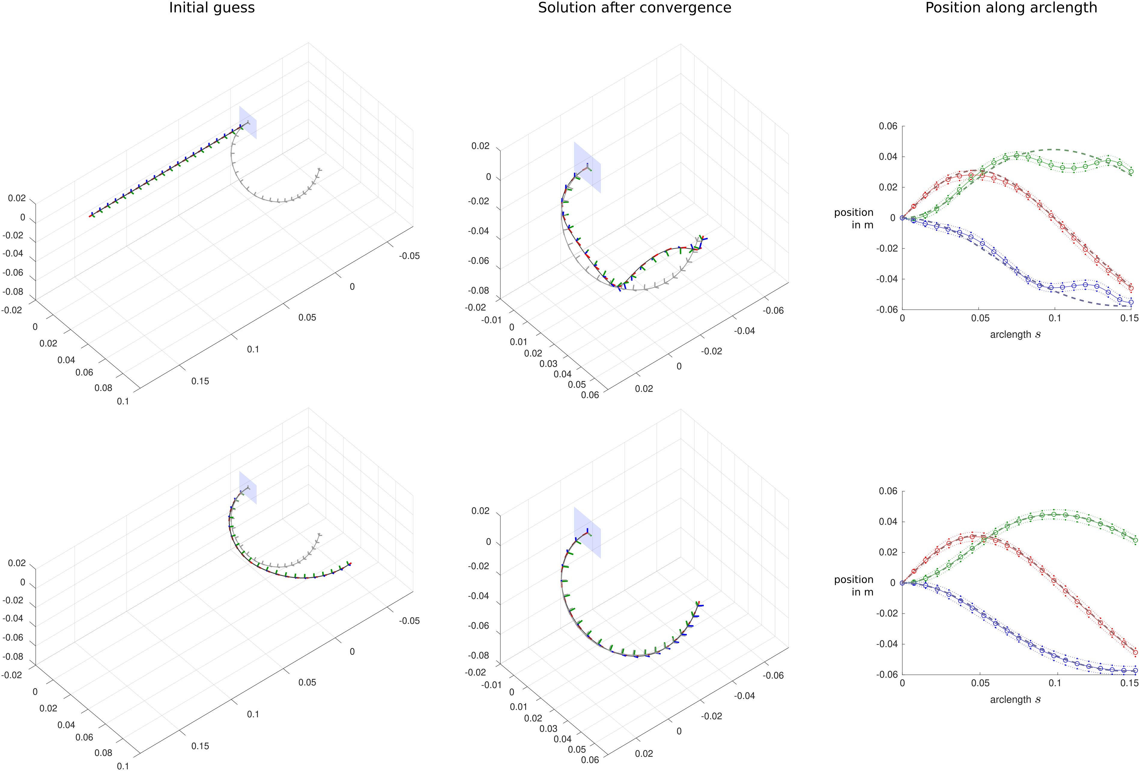
Finally, we would like to emphasize and acknowledge that our current prior is based on simplified assumptions, as it does not incorporate any knowledge about external or actuation forces. This knowledge could be incorporated in our prior by assuming a Gaussian process
5 Conclusion
This paper describes a state estimation approach for a continuum robot utilizing sparse Gaussian process regression. The proposed framework makes use of a simplified Cosserat rod formulation, making it applicable to a large variety of continuous manipulator, without requiring additional robot-dependent knowledge and information. By considering limited discrete sensor information, the approach allows for a continuous estimation of the robot’s full state, including backbone pose and internal strains as well as their respective uncertainty envelopes. Evaluation with simulations and real robot experiments show that accurate and continuous estimates of a continuum robot’s shape can be achieved, resulting in average end-effector errors between the estimated and ground truth shape of 3.5 mm and 0.016° in simulation or 3.3 mm and 0.035° during experiments for unloaded configurations and 6.2 mm and 0.041° for loaded ones, when using discrete pose measurements.
Future work could focus on extending the proposed approach to also include and estimate the second derivative of the backbone’s pose and position, which would enable estimation of the forces and moments acting on the robot structure. Furthermore, although we have demonstrated the method on a single continuum robot, we believe it will be possible to extend the method to parallel continuum robots quite easily where there are loops in the topology; by viewing this as a batch state estimation problem, we can again borrow ideas from mobile robotics to perform inference over topology graphs with loops.
Footnotes
Acknowledgments
We are indebted to Gabriele D’Eleuterio, also at the University of Toronto, for helpful discussions around the similarity between the rigid body and Cosserat equations expressed using
Declaration of conflicting interests
The author(s) declared no potential conflicts of interest with respect to the research, authorship, and/or publication of this article.
Funding
The author(s) disclosed receipt of the following financial support for the research, authorship, and/or publication of this article: This work was supported by the Natural Sciences and Engineering Research Council (NSERC) of Canada.