
Abstract
We develop an approach to improve the learning capabilities of robotic systems by combining learned predictive models with experience-based state-action policy mappings. Predictive models provide an understanding of the task and the dynamics, while experience-based (model-free) policy mappings encode favorable actions that override planned actions. We refer to our approach of systematically combining model-based and model-free learning methods as hybrid learning. Our approach efficiently learns motor skills and improves the performance of predictive models and experience-based policies. Moreover, our approach enables policies (both model-based and model-free) to be updated using any off-policy reinforcement learning method. We derive a deterministic method of hybrid learning by optimally switching between learning modalities. We adapt our method to a stochastic variation that relaxes some of the key assumptions in the original derivation. Our deterministic and stochastic variations are tested on a variety of robot control benchmark tasks in simulation as well as a hardware manipulation task. We extend our approach for use with imitation learning methods, where experience is provided through demonstrations, and we test the expanded capability with a real-world pick-and-place task. The results show that our method is capable of improving the performance and sample efficiency of learning motor skills in a variety of experimental domains.
1. Introduction
Reinforcement learning (RL) algorithms can generally be divided into two categories—model-free and model-based. Model-free methods avoid the need to model the environment or dynamics by learning a direct policy mapping between states and actions (Schulman et al., 2017; Haarnoja et al., 2018a,b). The policy is learned through experience, so we consider model-free methods to be “experience-based.” Model-based methods typically learn a dynamics model and a reward function to predict the next state and next reward given the current state and a potential next action. These outputs can be sequentially used to predict into the future the expected rewards for a set of actions. These methods have contrasting strengths and weaknesses. Model-free approaches require significantly more data and diverse experience to learn the task than model-based methods (Chua et al., 2018), but model-free approaches often produce better performance than model-based methods. The prediction capabilities of model-based methods make them more “sample-efficient” in solving robot learning tasks (Williams et al., 2017; Chua et al., 2018; Abraham et al., 2020), but the models are often highly complex and can require special structure (Nagabandi et al., 2018; Havens et al., 2019; Sharma et al., 2019; Abraham et al., 2020; Abraham et al., 2017; Abraham and Murphey, 2019). Is there a way to leverage the beneficial aspects of each of these methods to enable robotic systems to rapidly learn tasks with a limited amount of experience?
Recent work tries to address this question by exploring alternate ways of structuring environment models by combining probabilistic models with deterministic components (Chua et al., 2018). Other work has explored using latent-space representations to reduce model complexity (Havens et al., 2019; Sharma et al., 2019). Related methods use high fidelity Gaussian Processes to create models, but these methods are limited by the amount of data that can be collected (Deisenroth and Rasmussen, 2011). Finally, some researchers try to improve experience-based methods by adding exploration as part of the objective (Pathak et al., 2017). However, all of these approaches focus on improving either model-based or model-free methods separately rather than combining model-based planning with experience-based learning.
Methods that combine model-based planning and experience-based learning tend to do so in stages (Chebotar et al., 2017; Bansal et al., 2017; Nagabandi et al., 2018). First, a model is used to collect data for a task to jump-start the learning process. Then, supervised learning is used to update a policy (Levine and Abbeel, 2014; Chebotar et al., 2017) or an experience-based method is used to continue the learning from that stage (Nagabandi et al., 2018). Moreover, the model is often used as an oracle, which provides labels to a base policy. The aim of these methods is to train a policy that does not rely on the model after training. While these approaches do improve learning, they do not algorithmically leverage the two learning approaches in an optimal manner, resulting in objective mismatch (Lambert et al., 2020). The sequential optimization solves two different problems; the model-based controller seeks to improve the objective, while the policy seeks to match the model-based controller.
Our approach algorithmically combines model-based and experience-based learning by using the learned model to predict how well an experience-based policy will behave, and then optimally update the resulting actions. Using hybrid control as the foundation for our approach, we derive a controller that optimally uses model-based actions when the policy is uncertain, and allows the algorithm to fall back on the experience-based policy when there is high confidence that the actions will result in a favorable outcome. As a result, our approach does not rely on improving the model (but can easily integrate high fidelity models), but instead optimally combines the actions generated from model-based and experience-based methods to achieve high performance in the specified task. Our contributions in this work can be summarized as follows: • We present a hybrid control theoretic approach to robot learning motor skills. • We derive deterministic and stochastic algorithmic formulations of our proposed hybrid learning approach. • We introduce a measure for determining the agreement between learned model and policy. • We demonstrate the flexibility of our approach with various learning approaches such as off-policy reinforcement learning (Haarnoja et al., 2018a) and behavior cloning (Pomerleau, 1998). • We demonstrate improved sample efficiency and task performance over state-of-the-art model-based methods (Ansari and Murphey, 2016; Williams et al., 2017), model-free methods (Haarnoja et al., 2018b), and methods that combine model-based and model-free methods (Feinberg et al., 2018; Buckman et al., 2018; Janner et al., 2019; Montgomery and Levine, 2016; Nagabandi et al., 2018).
The paper is structured as follows: Section 2 provides background knowledge of the problem statement and its formulation; Section 3 introduces our approach and derives both deterministic and stochastic formulations of our algorithm; Section 4 provides simulated results and comparisons as well as experimental validation of our approach; Section 5 provides comparisons to related work that combines model-based and model-free methods; and Section 6 concludes the work and discusses future work.
2. Background
In this work, we build on the framework of Markov Decision Processes (MDP) and aspects of hybrid control theory. Robot reinforcement learning problems are often formulated as MDPs. The MDP formulation assumes the Markov property—that the result of an action taken in a given state only depends on the current state and does not depend on the prior history. The Markov property applies to both model-based and model-free methods, which are used in this work. Prior work which combines model-free and model-based methods often relies on hand-tuned objective functions or ultimately solves two different objective functions for the different learning methods. In this work, we introduce hybrid control theory as a structured approach to combining multiple control strategies with a single objective function.
Markov decision processes
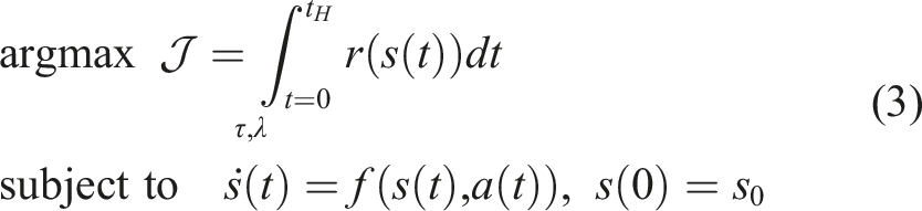
A Markov Decision Process (MDP) is a mathematical framework for a discrete-time stochastic process. The goal of the MDP formulation is to find a mapping from state to action that maximizes the total reward acquired from interacting in an environment for some fixed amount of time. An MDP can be represented as

Model-free approaches learn a stochastic policy a ∼ π(· | s) that maximizes the reward r at a state s. Model-based approaches solve the MDP problem by modeling a transition function st+1 = f(s t , a t ) and a reward function r t = r(s t ) 1 . Model-based methods either use these functions to construct a policy or directly generate actions through model-based planning (Chua et al., 2018). When the transition model and the reward function are known, the MDP formulation becomes an optimal control problem. We can use any set of existing methods (Li and Todorov, 2004; Tang et al., 2018) to solve for the best set of actions (or policy) to maximize the reward 2 .
Hybrid control theory for mode scheduling
In mode scheduling problems, the goal is to maximize a reward function through the synthesis of two (or more) control strategies. A common example of mode switching is when a vertical takeoff and landing vehicle switches from flight mode to landing mode. In hybrid control theory, these control strategies are often called modes. Thus, mode switching can also be called policy switching (Axelsson et al., 2008; Vasudevan et al., 2013). We can use hybrid control theory to determine the optimal time to switch from one control policy to another. Most mode scheduling problems are formulated in continuous time and are subject to dynamics of the form

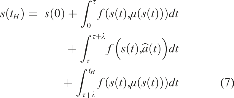
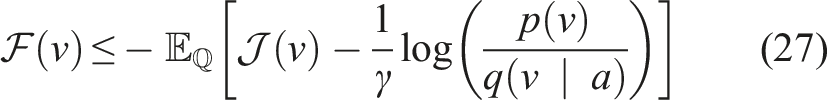
The continuous time dynamics function requires us to reformulate the objective function from (1). First, we introduce an objective function as a deterministic function of the state and control
3. Hybrid learning
The goal of this section is to introduce hybrid learning as a method for optimally synthesizing model-based and model-free learning methods. In Section 2, we introduced Markov Decision Processes and described how model-based and model-free methods follow the MDP formulation. Although both methods assume an underlying MDP, only the model-based method learns this transition probability. The transition probability is a key feature linking the MDP formulation to hybrid control theory. Most mode scheduling problems are constrained by a dynamics function, which governs the transition from a current state s t to a next state st+1 given a current action a t . Thus, the MDP transition probability and the mode scheduling dynamics function have the same form. In this work, we use the model-based prediction capability to develop a hybrid control approach to determine the optimal time to switch from the action specified by experience-based policy to an alternate model-based action.
We first introduce a deterministic formulation of the algorithm with theoretical proofs describing the foundations of our method. We then derive a stochastic method as a way to relax the assumptions made in the deterministic formulation. In both the deterministic and stochastic formulations, we solve the learning problem indirectly. We break down the overall learning problem into solvable sub-problems, which collectively imply the original learning problem has been solved. Finally, we extend our method to use expert demonstrations as experience. Both the deterministic and stochastic approaches can be improved by providing informative experience in the form of expert demonstrations.
3.1. Deterministic method
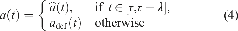
Consider a continuous time MDP formulation of the objective in (3) and the dynamics in (2), where f and r are learned using arbitrary regression methods (e.g., neural network least squares, Gaussian processes), and the experience-based policy π is learned through a model-free approach (e.g., policy gradient (Sutton et al., 2000)). We assume the learned policy has the form
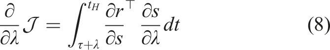
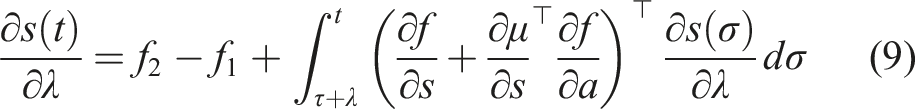
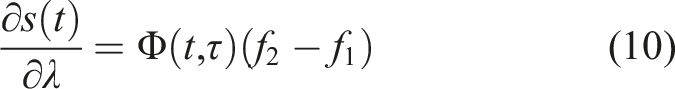
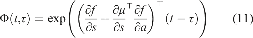
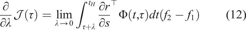
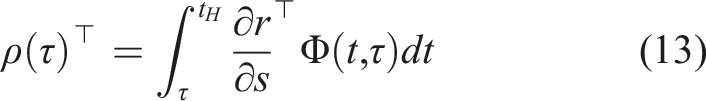
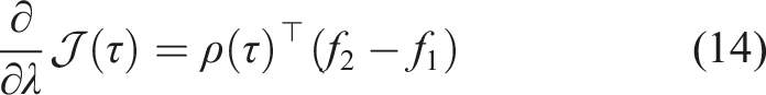
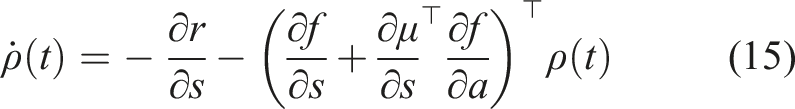
Assume f, r, and μ are differentiable and continuous in time. The sensitivity of the objective in (3) with respect to the duration time λ of switching from μ(s) to
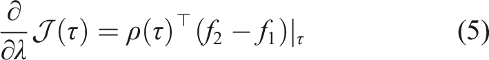
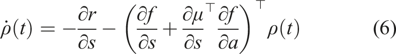
First, we define the trajectory Lemma 1 gives us the proof and definition of the mode insertion gradient (5). The mode insertion gradient tells us the change in the objective function when switching from the default policy behavior μ to some other arbitrarily defined control Given a suboptimal policy π, what is the best action the robot can take to maximize the objective in (3), at any time t ∈ [0, t
H
], subject to the uncertainty (or certainty) of the policy defined by Σ(s)? We approach this new sub-problem by specifying the auxiliary optimization problem
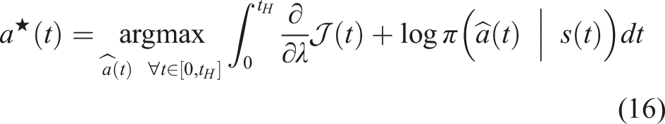
Assuming f, r, and π are continuous and differentiable in s, a and t, the best possible action to improve the performance of (3) and is a solution to (16) for any time t ∈ [0, t
H
] is

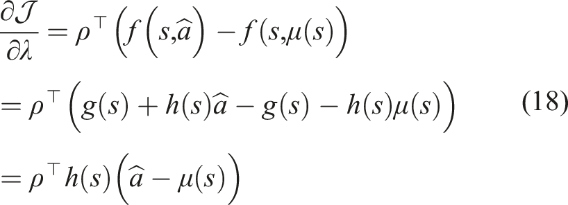
The mode insertion gradient can be rewritten (5) as The proof in Theorem 1 provides the best action a robotic system can take given a default experience-based policy. Each action generated uses the sensitivity of changing the objective based on the predictive model’s behavior while relying on the experience-based policy to regulate when the model information will be useful. We convert the result in Theorem 1 into our first algorithm, a deterministic approach to hybrid learning (see Alg. 1). With the proposed approach, we are able to numerically determine the contribution of the learned predictive models towards improving the task. We show (17) provides the best possible action given the current belief of the dynamics f and the task reward r. Next, we use the control Hamiltonian to show we can find a local optima of the objective in (17).


Hybrid Learning (Deterministic) 1: Randomly initialize continuous differentiable models f(s, a), r(s, a) with parameters ψ and policy π(a | s) with parameter θ. Initialize memory buffer 2: 3: reset environment and exploration noise ɛ 4: 5: observe state s(t
i
) ▷ simulation loop 6: ▷ forward predict states using any integration method (Euler shown) 7: s(τi+1) = s(τ
i
) + f(s(τ
i
), μ(s(τ
i
)))dt 8: r(τ
i
) = r(s(τ
i
), μ(s(τ
i
))) 9: ▷ backwards integrate 10: ρ(t
i
+ t
H
) = 11: 12: 13: 14: 15: 16: apply to robot 17: append data 18: ▷ Update model and policy
5
19: Update f, r by sampling N data points from 20: Update π using any experience-based method 21:
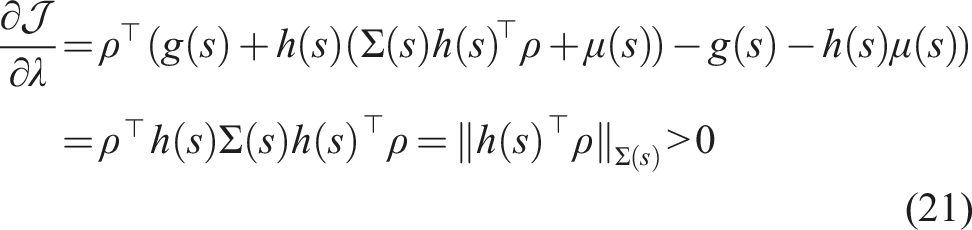
Assuming
Inserting (17) into (5) yields Corollary 1 tells us the action defined in (17) generates the best action to improve the performance of the robot given valid learned models. Corollary 1 also states that if the policy is already a solution, then our approach for hybrid learning does not modify the known solution and simply returns the policy’s action. The preceding proofs have a strict requirement of continuity and differentiability of the learned models and the policy. As these constraints are not always possible and often learned models have noisy derivatives, our goal is to try to reformulate the objective in (3) into an equivalent problem that can be solved without these strict assumptions. One approach is to reformulate the problem in discrete time as an expectation. This formulation is introduced in the following section.
3.2. Stochastic method
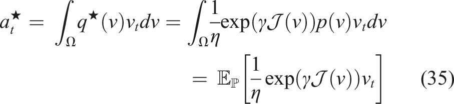
For the stochastic approach, we relax the continuity, differentiability, and continuous-time restrictions specified in the deterministic objective in (3) by first restating the objective as an expectation

We find the best augmented action by defining two distributions
Following the work in Williams et al. (2017), we use Jensen’s inequality and importance sampling on the free-energy definition (Theodorou and Todorov, 2012) of the control system using distribution
Now, we can define an optimal distribution
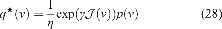
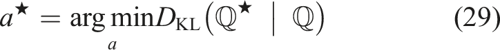
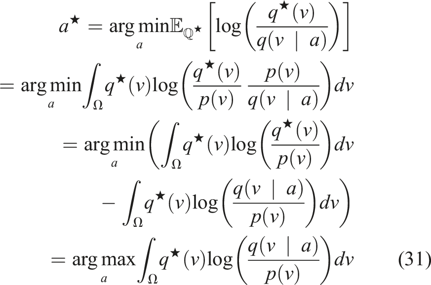
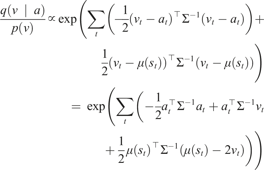
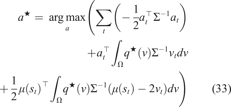
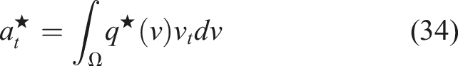
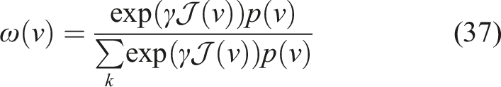
Returning to our original problem of how to find the best actions to augmented π and improve the objective in (23), we now we want to construct a distribution to augment the policy distribution p(v) and improve the objective.
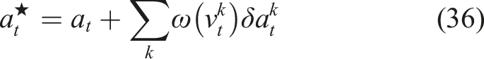
The recursive, sample-based, solution to (29) is
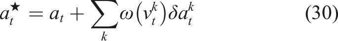
Expanding the objective in (29), we can show Using the change of variable v
t
= a
t
+ δa
t
, we get the recursive, sample-based solution
Hybrid Learning (Stochastic) 1: Randomly initialize continuous differentiable models f(s, a), r(s, a) with parameters ψ and policy π(a | s) with parameter θ. Initialize memory buffer 2: 3: reset environment 4: 5: observe state s
t
▷ simulation loop 6: 7: 8: ▷ forward predict state and reward 9: 10: 11: 12: ▷ update actions 13: 14: 15: 16: 17: 18: 19: apply a0 to robot 20: append data 21: ▷ Update model and policy
8
22: Update f, r by sampling N data points from 23: Update π using any experience-based method 24:
3.3. Imitation learning
One limitation of reinforcement learning approaches is the large amount of data required for training—even for sample-efficient methods. Both the deterministic and stochastic hybrid learning approaches could be improved by being provided with informative, expert demonstrations of the task. Therefore, we extend our method to use expert demonstrations as experience. Imitation learning (Argall et al., 2009; Ross and Bagnell, 2010) focuses on using expert demonstrations to either mimic a task or to initialize learning complex data-intensive tasks. We use imitation learning, specifically behavior cloning, as an initialization for how a robot should accomplish a task. Hybrid learning as described in Section 3.1 and 3.2 is then used as a method to embed model-based information to compensate for the uncertainty in the learned policy, improving the overall performance through planning. We outline the algorithmic implementation hybrid learning with behavior cloning in Appendix C.
4. Experiments
This section compares the previously described methodology to state-of-the-art model-based and model-free methods. First, we evaluate our deterministic and stochastic variations on a range of simulated benchmark control tasks from OpenAI Gym (Brockman et al., 2016). Then, we extend the evaluation of our stochastic method to the real world with a robotic arm manipulation experiment. Finally, we present two behavior cloning experiments; one experiment uses an OpenAI Gym environment, and the other demonstrates a real-world pick-and-place experiment with a robotic arm. All implementation details are included in Appendix B. Each experiment shown in this section was trained on ten different random seeds. Unless otherwise stated, the solid curves in the following figures correspond to the mean, and the shaded regions correspond to the standard deviation over the ten trials. 9
4.1. Simulated benchmarks
We evaluate our approach on a subset of environments from the OpenAI Gym benchmarks (Brockman et al., 2016). Specifically, we look at the cartpole swingup environment, the Acrobot swingup environment, the hopper environment, and the half-cheetah environment, which are described in more detail in Appendix B. We evaluate our proposed approach on common RL benchmarks to verify our measure for model and policy alignment. In particular, the goal is to show that our method (1) is more sample efficient, (2) obtains higher rewards than the comparison methods even though it is a model-based RL method, and (3) improves the performance of the individual model and policy that are being learned over time.
Deterministic results
We compare our hybrid learning approach to model-based method in Ansari and Murphey (2016) and model-free method (Soft Actor-Critic) in Haarnoja et al. (2018b).
While model-free methods have exploration naturally encoded in their formulation, the deterministic model-based and hybrid learning approaches require added exploration noise to induce exploring other regions of state space. Figure 1 summarizes our deterministic benchmark results. The top row shows snapshots of each Gym environment. The middle row shows that our method outperforms both the model-based and model-free methods for all four tested environments. Our hybrid learning approach uses the confidence bounds generated by the stochastic policy to infer when best to rely on the policy or predictive models. As a result, hybrid learning enables learning in unstructured environments comparable to model-free methods with the sample efficiency of model-based learning approaches. For the swingup tasks, the model-based method learns the task but converges to a less optimal policy than our hybrid approach. For the locomotion tasks, the model-based method suffers from its inability to model discontinuous dynamics. Performance curves of our proposed deterministic hybrid learning algorithm on multiple environments during training (averaged over 10 random seeds). All methods use the same structured learning models. Our method is shown to improve the model-based benchmark results (due to the use of experience-based methods) while maintaining significant improvements on the number of interactions necessary with the environment to obtain those results. The mode insertion gradient is also shown for each example which illustrates the model-policy agreement over time. Note: Markers are included for distinguishing between methods only and do not represent all data points.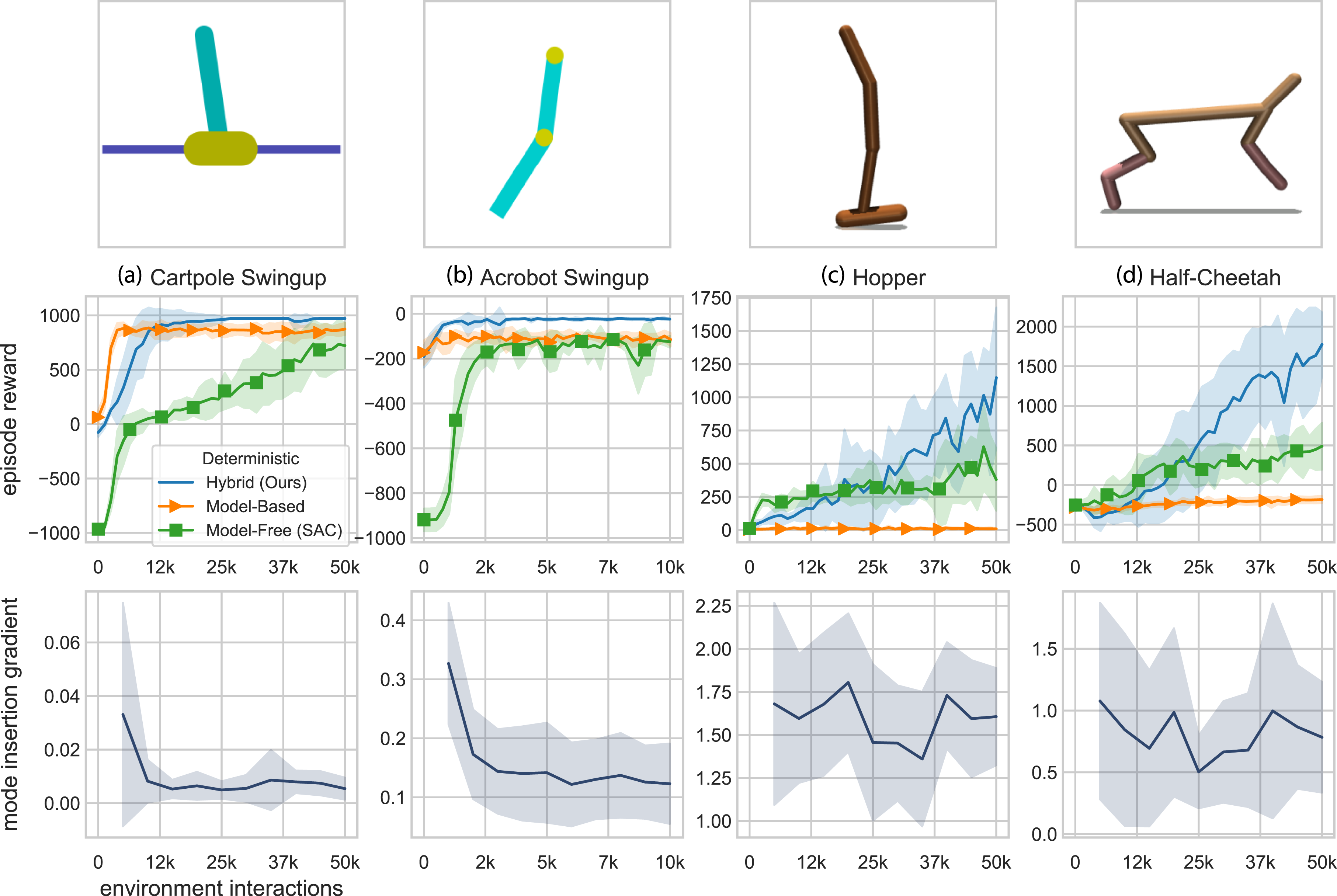
The bottom row shows the mode insertion gradient for the hybrid learning method for each environment. The mode insertion gradient can be interpreted as a measure of agreement between the policy and the learned model. The swingup examples show an eventual reduction in the mode insertion gradient. We interpret this as the convergence of the learned model and policy. The locomotion examples do not converge in the number of environment interactions observed. The lack of convergence indicates that the learning process has not yet stabilized, which is consistent with the episode rewards learning curves (in the middle row).
Stochastic results
We next compare the stochastic formulation of hybrid learning to a stochastic neural network model-based controller (NN-MPPI) (Williams et al., 2017) and the same model-free controller as the deterministic formulation (SAC) (Haarnoja et al., 2018b). The goal of these experiments is to show that this hybrid learning formulation still outperforms these state-of-the-art learning techniques without imposing continuity and differentiability requirements. Figure 2 summarizes our stochastic benchmark results. The model-free parameters are held constant from the deterministic results to remove any impact of hyperparameter tuning. Figure 2 shows that for both swingup tasks, the stochastic formulation outperforms the model-free method but performs similarly to the improved model-based method. Even with the improved model-based method, the model-based method converges to a less optimal policy for the Acrobot than our hybrid approach. For the locomotion tasks, our stochastic formulation maintains the improved performance and sample efficiency over the model-based method and the model-free method. Exploration is naturally encoded into the stochastic algorithm, which results in more stable learning when there is uncertainty in the task. Performance curves of our proposed stochastic hybrid learning algorithm on multiple environments during training (averaged over 10 random seeds). Our approach improves both the sample efficiency and the highest expected reward. Note: Markers are included for distinguishing between methods only and do not represent all data points.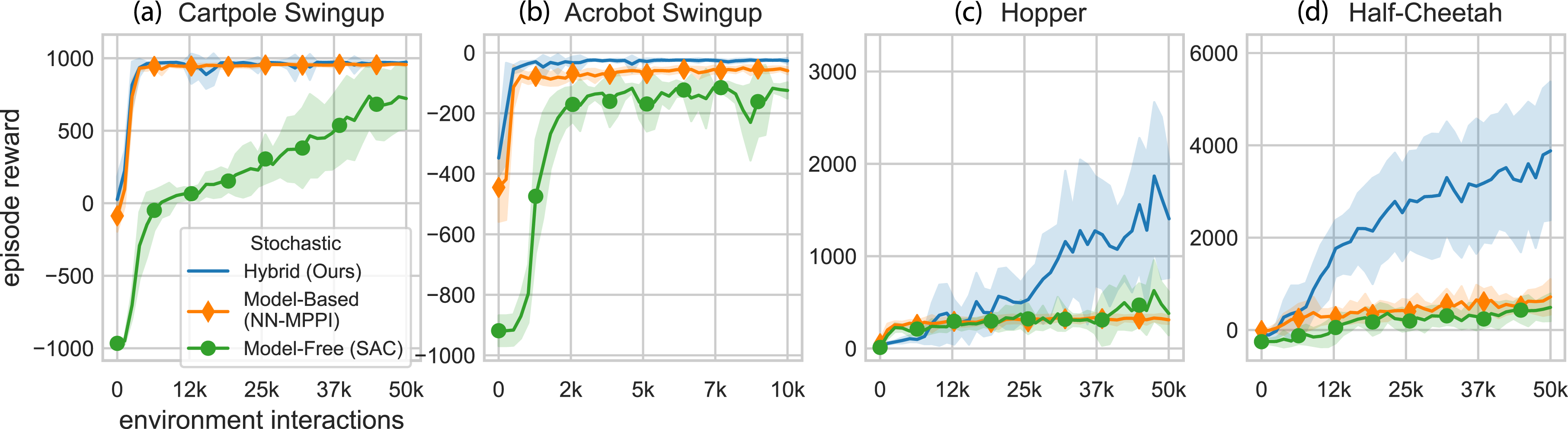
Although we no longer have a mode insertion gradient for the stochastic method, we can analyze the individual learned model and policy obtained from hybrid learning. In Figure 3, both the environment interactions and episode rewards are normalized to allow comparisons between the different environments. For all environments, hybrid learning is shown to improve the learning capabilities of both the learned predictive model and the policy through the hybrid control approach. The policy is “filtered” through the learned model and augmented, allowing the robotic system to be guided by both the prediction and experience. Thus, both the predictive model and the policy benefit ultimately performing better as a standalone approach using hybrid learning. Figure 3 shows that for different tasks, the model and policy learn at different rates, but both evolve over time with our hybrid learning approach. Comparison of model and policy evolution during stochastic hybrid learning. Episode rewards and environment interactions have been normalized to allow comparisons between different environments. For the swingup tasks, both the models and policies quickly learn the task. For the locomotion tasks, models also learn over the course of training, but the policies learn at a faster rate. These plots show that the hybrid learning approach pushes performance of both the model and the policy. Note: Markers are included for distinguishing between methods only and do not represent all data points.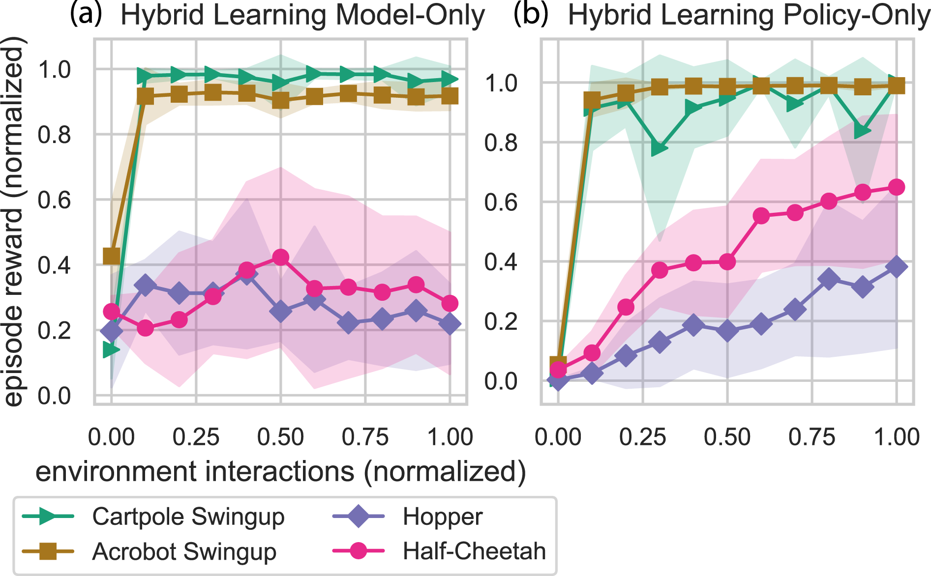
Comparisons
We can compare learned models and policies at 50,000 steps for both the deterministic and stochastic implementations. Figure 4 shows 10 tests of each final model-based, model-free, and hybrid learning method. In addition to the full hybrid method, we show the individual model-based and model-free policies trained during hybrid learning as “Hybrid Learning Model-Only” and “Hybrid Learning Policy-Only,” respectively. In addition to having greater performance with the full implementation of hybrid learning, our approach tends to push the performance of both the model and policy. For the swingup tasks, the model-based method outperformed the hybrid model-only evaluation, but both the full hybrid learning and hybrid policy-only evaluations outperform all other methods. This result indicates that the hybrid learning approach does not require model improvements once it has learned a “good enough” model. For the locomotion tasks, the deterministic policy-only hybrid learning on average outperforms the deterministic full hybrid learning approach. For the stochastic method, the results are reversed with the full hybrid learning approach outperforming the policy-only approach. These results indicate that if the goal is to produce animations in simulation, the policy-only controller is likely sufficient to control the simulation. If the goal is to control real-world systems with uncertainty, maintaining the full hybrid controller allows continued benefit from the learned predictive model and experience-based policy. Comparison of final model-based and model-free policies for both deterministic and stochastic methods. For the hybrid learning method, we show the final model-only and policy-only results separately as well as in combination. Each boxplot displays the results of 100 tests (10 seeds, 10 episodes each). The interquartile region (IQR) contains 50% of the data (from Q1 to Q3) and is shown as a filled box with notches at the median. The whiskers span [Q1 - 1.5×IQR, Q3 + 1.5×IQR]. Any data points falling outside the whiskers are designated as outliers and are shown as unfilled circles. The means are shown as white circles. For all methods, the hybrid policy-only and full hybrid learning outperform all other methods.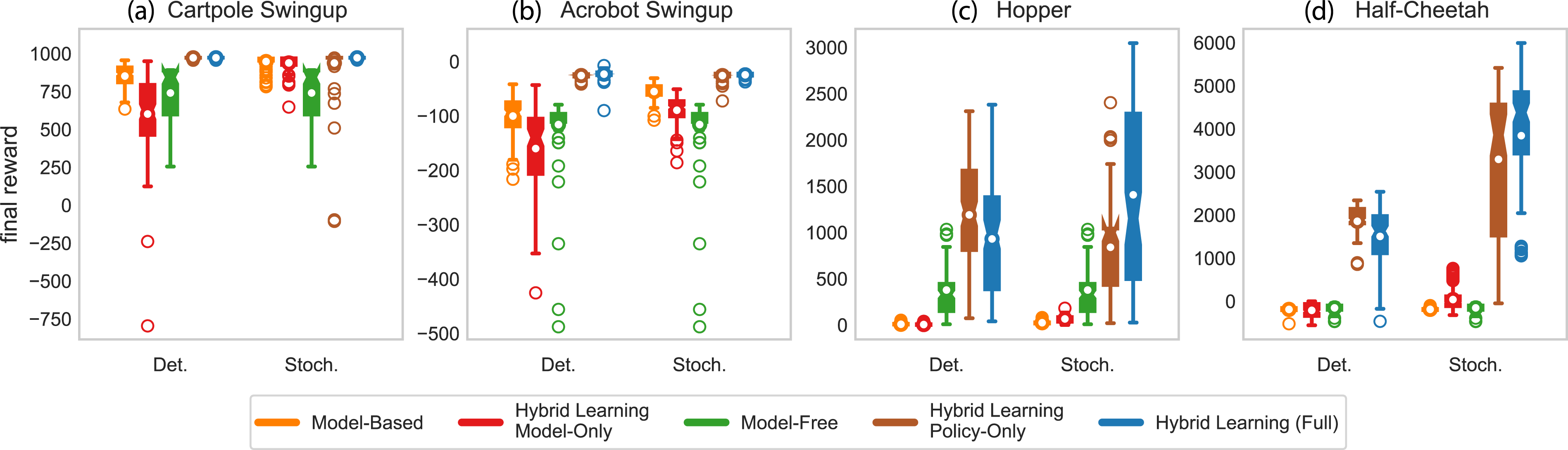
4.2. Robot learning from experience
Next, we apply hybrid learning to an experiment with a Sawyer robot to validate hybrid learning for real robot tasks. For this experiment, the goal is for the robot to access a block surrounded by clutter. The true positions of the “clutter” blocks and the “target” block are unknown to the robot. The robot’s state is comprised of vectors from the robot’s end-effector to each block. The “target” block is always placed in the same start location, but the “clutter” blocks are randomly placed around the “target” block. The robot is rewarded for pushing the “clutter” blocks out of the way and accessing the “target” block (see Figure 5 for task illustration). Hybrid learning results on the Sawyer robot (averaged over 10 trials). The time series on the right provides a visualization of the task. The task is to access a target block (shown in green) surrounded by clutter (five other blocks) through environment interactions. Our stochastic hybrid learning method is able to achieve the task by effectively using both predictive models and experience-based methods. For additional visualization, see Extension 1. Note: Markers are included for distinguishing between methods only and do not represent all data points.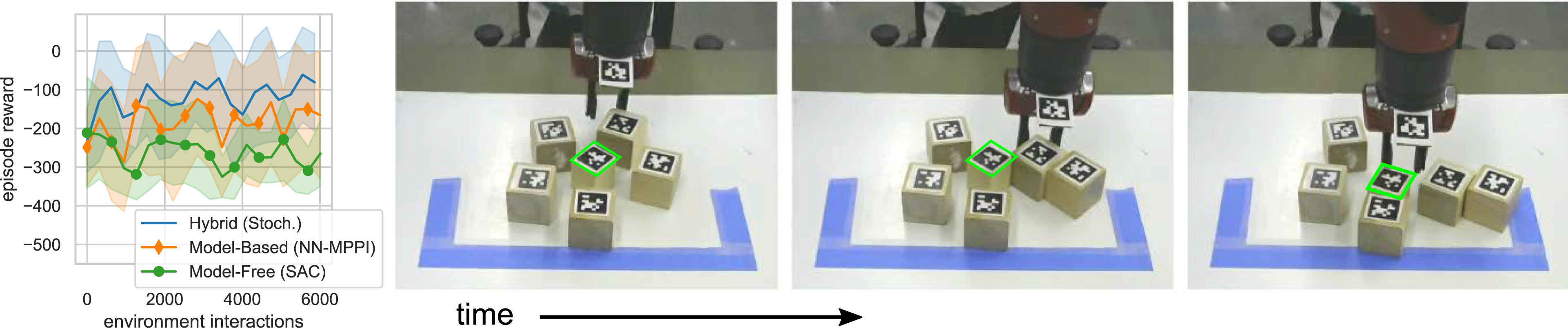
What makes this task difficult is that the robot must learn to push the “clutter” blocks out of the way rather than directly reaching towards the “target” block. Since our method naturally relies on the predictive models when the policy is uncertain, the robot is able to plan through the clutter to achieve the task. Figure 5 shows that our proposed hybrid learning approach outperforms both the model-based and model-free methods. During testing, we observed that the model-based approach tries to directly “reach” for the block without first clearing the clutter, which often results in pushing the target block outside workspace. Although the model-free method rarely pushes the block outside the workspace, it takes significantly longer for the model-free method to discover the pushing dynamics. Our hybrid approach learns to push the clutter blocks out of the way before accessing the target block. These tactics can also be viewed in Extension 1.
4.3. Behavior cloning
The final set of experiments illustrates our algorithm with imitation learning. For both experiments, expert demonstrations are used to generate the experience-based policy through behavior cloning and the learned predictive models adapt to the uncertainty in the policy.
Simulated benchmark results
We test hybrid imitation on the 3D Pybullet Ant environment (Coumans and Bai, 2016). The goal is for the four legged ant to run as far as it can to the right (from the viewer’s perspective) within the allotted time. At each iteration, we provide the agent with an expert demonstration generated from a Proximal Policy Optimization (PPO) (Schulman et al., 2017) solution. Each demonstration is used to construct a predictive model as well as a policy (through behavior cloning). The stochastic hybrid learning approach is used to plan and test the robot’s performance in the environment. Environment experience is then used to update the predictive models while the expert demonstrations are solely used to update the policy.
In Figure 6, we compare hybrid learning against behavior cloning. Our method is able to achieve the task at the level of the expert within six (200 step) demonstrations, where the behavior cloned policy is unable to achieve the expert performance. Interestingly, the ant environment is less susceptible to the covariate shift problem (where the state distribution generated by the expert policy does not match the distribution of states generated by the imitated policy (Ross and Bagnell, 2010), which is common in behavior cloning. This suggests that the ant experiences a significantly large distribution of states during the expert demonstration. However, the resulting performance for the behavior cloning is worse than that of the expert. Our approach is able to achieve similar performance as behavior cloning with roughly two fewer demonstrations and performs just as well as the expert demonstrations. Results for hybrid stochastic control with behavior cloned policies (averaged over 10 trials) using the Ant Pybullet environment (shown right). Expert demonstrations (actions executed by an expert policy on the ant robot) are used as experience to boot-strap a learned stochastic policy (behavior cloning) in addition to predictive models which encode the dynamics and the underlying task of the ant. Our method is able to adapt the expert experience to the predictive models, improving the performance of behavior cloning and performing as well as the expert. Note: Markers are included for distinguishing between methods only and do not represent all data points.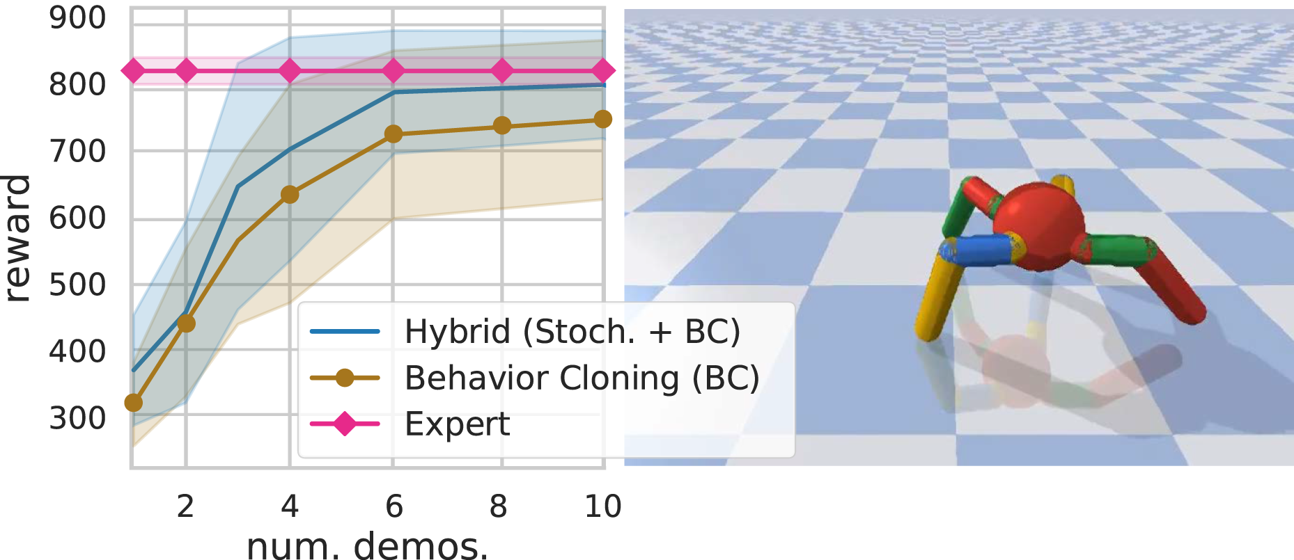
Robot learning from examples results
We also test our approach on a pick-and-place experiment with the Franka Panda robot. The real hardware system is more likely to have the covariate shift problem. The goal for the robot is to learn how to stack one block on top of another block using demonstrations (see Figure 7). As with the ant simulated example in Figure 6, a demonstration is provided at each attempt at the task and is used to update the learned models. Experience obtained in the environment is solely used to update the predictive models. We use a total of ten precollected demonstrations of the block stacking example (given one at a time to the behavior cloning algorithm before testing). At each testing time, the robot arm is initialized at the same spot over the initial block. Since the demonstrations vary around the arm’s initial position, any state drift is a result of the generated imitated actions and will result in the covariate shift problem leading to poor performance. Hybrid learning with behavior cloning results on the Franka Panda robot (averaged over 5 trials). The time series on the right provides a visualization of the task. The task is to stack a block on top of another using expert demonstrations. Our method is able to learn the block stacking task within three expert demonstrations and provides solutions that are more repeatable than with behavior cloning. For additional visualization, see Extension 1. Note: Markers are included for distinguishing between methods only and do not represent all data points.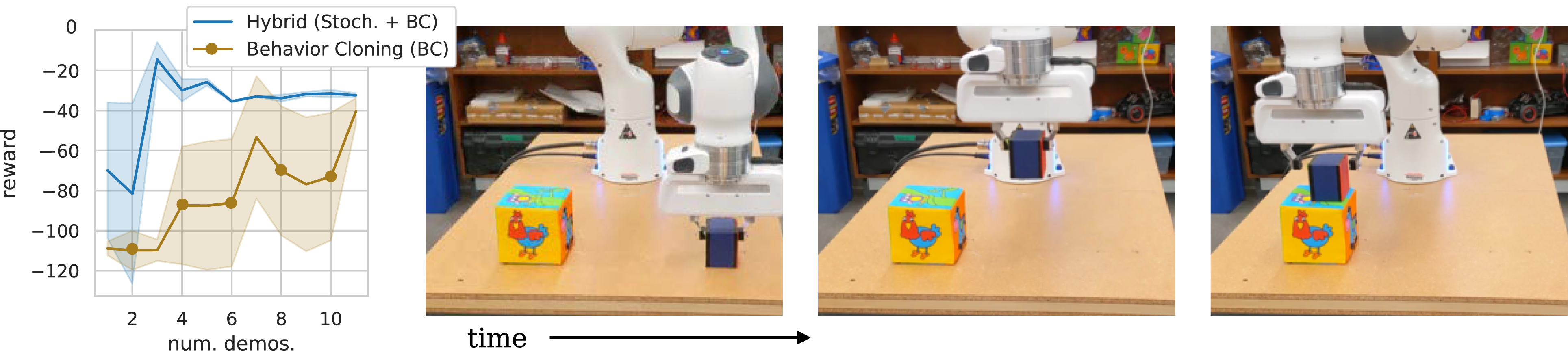
Figure 7 shows our approach is capable of learning the task in as little as two demonstrations where behavior cloning suffers from poor performance. Since our approach synthesizes actions when the policy is uncertain, the robot is able to interpolate between regions where the expert demonstration was lacking, enabling the robot to achieve the task.
5. Related work
Our hybrid learning approach is able to leverage both the model and the policy during both training and real-time operation. This is a major difference between our approach and other reinforcement learning methods which combine model-based and model-free approaches. Many of the approaches in related work only use the model to help the model-free policy learn better, but do not have any use for the model once the model-free policy training is complete.
Model-Based Value Expansion (MVE) (Feinberg et al., 2018), Stochastic Ensemble Value Expansion (STEVE) (Buckman et al., 2018), and Model Based Policy Optimization (MBPO) (Janner et al., 2019) use only the model-free policy to interact with the environment both during training and after training. The model is learned offline using data accumulated by the model-free policy, but there is no model-based controller associated with the model. Instead, the policy is used to “imagine” future transitions in the model-based environment for short rollouts. These model rollouts are used during the update step to augment Q-learning (for MVE and STEVE) or the policy directly (for MBPO).
Guided Policy Search (GPS) (Montgomery and Levine, 2016) takes a different approach by using a model-based controller to interact with the environment. Each iteration, GPS fits a dynamics model to the most recently collected data, and then uses these models to constrain the policy updates. In this algorithm, only the model-based controller interacts with the environment during training, and the goal is to train a policy which can be used without the model after training.
Model-based learning with model-free fine-tuning (MB-MF) (Nagabandi et al., 2018) takes another approach. First, a model-based random shooting controller is used to learn a coarse-grained representation of the dynamics. Then, the learned dynamics are transferred to a model-free method via data aggregation. Finally, the model-free policy is fine-tuned through interactions with the environment. Both the model-based controller and the model-free policy interact with the environment, but they do so sequentially—during any given trial, only one of them plays a role. Although the model is no longer needed once the model-free policy is trained, the idea with this algorithm is that the model could be reused to learn another task with the same agent without needing to relearn a model, similar to the method we present here.
In Figure 8, we tested the stochastic hybrid learning algorithm and other methods which combine model-based and model-free learning. Details of the comparison methods can be found in Appendix D. The results show that the methods we present here outperform these related methods. In addition to the learning gains, the hybrid learning controller presented here maintains both the model and the policy after training. This may provide benefits during future controller execution—if the hybrid learning trained policy encounters an untested state during operation, it will have the model-based controller to fall back on to compensate for this uncertainty. Comparison to related work combining model-based and model-free methods (averaged over 10 random seeds). Our approach improves both the sample efficiency and the highest expected reward. Additional details and pairwise comparisons are included in Appendix. Note: Markers are included for distinguishing between methods only and do not represent all data points.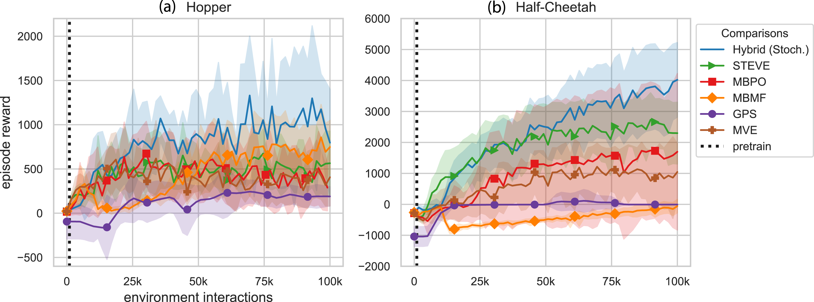
6. Conclusion
In this work, we present hybrid learning as a method for formally combining model-based learning with experience-based policy learning based on hybrid control theory. Our approach derives the best action a robotic agent can take given the learned models, both model-free and model-based. We tested our approach in various simulated and real-world environments using a variety of learning conditions and show that our method improves both the sample efficiency and the resulting performance of learning motor skills.
Future directions of this work will focus on testing real-world applications of hybrid learning. Our robot arm experiments demonstrated the ability of agents to learn online in a relatively simple physical test environment. In our Sawyer testing, the state was simplified to include the locations of each object relative to the end-effector. Future work could represent the state as an image and extend hybrid learning to visuo-motor tasks. Or the state could be expanded to include additional sensors such as contact sensors, accelerometers, etc. Our hybrid learning framework will enable extensive hardware testing–due to its real-time implementation–to determine how learning performance changes when adding new sensors into the state space and when modifying reward functions.
Key considerations for real-world testing are safety, time, and memory. Future work will explore methods of imposing safety constraints during operation. The time required to determine the next candidate action is dependent on the prediction horizon, the network sizes, and the number of candidate samples (for stochastic hybrid learning). As these variables increase, parallel processing will eventually be necessary.
Currently, exploration is done through random sampling. Future work will explore methods of incorporating exploration goals into the algorithm. As the state-space grows, random sampling may no longer be sufficient to span the state-space. Alternate forms of exploration could help reduce the number of candidate samples required and reduce computation time.
As computation and memory allow, particularly if parallel processing has been introduced for other reasons, it would be useful to explore model-based control using ensembles. One potential approach could train an ensemble of models and use the model uncertainty to determine which model-based controller to fall back on when the policy is uncertain. In general, bringing the robustness benefits of techniques such as path integral control (Williams et al., 2018) to our method can only improve its overall performance, but there may be many approaches that would all be equally viable.
Supplemental Material
Footnotes
Declaration of conflicting interests
The author(s) declared no potential conflicts of interest with respect to the research, authorship, and/or publication of this article.
Funding
The author(s) disclosed receipt of the following financial support for the research, authorship, and/or publication of this article: This material is based upon work supported by the National Science Foundation under Grant CNS 1837515 and Office of Naval Research under Grant N00014-21-1-2706. Any opinions, findings, and conclusions or recommendations expressed in this material are those of the authors and do not necessarily reflect the views of the aforementioned institutions.
Supplemental Material
Supplemental material for this article is available online.
Notes
Index to Multimedia Extension
Extension
Media Type
Description
1
Video
Overview of contributions and visualization of real-world robot experiments
Implementation Details
General Implementation Details: All simulated examples use the reward functions specified in the Pybullet (Coumans and Bai, 2016), Roboschool (OpenAI, 2017), or MuJoCo environments (Todorov et al., 2012) unless otherwise specified. Table A1 provides a list of all hyperparameters used for each environment tested. Any parameter not explicitly mentioned as deterministic or stochastic formulations of hybrid learning are equivalent. Parameters for all examples used in the paper (only when applicable). Each example using the deterministic formulation of hybrid learning (Alg. 1) uses added action exploration of the form ϵ = 0.999
t
where t is the total number of environment interactions.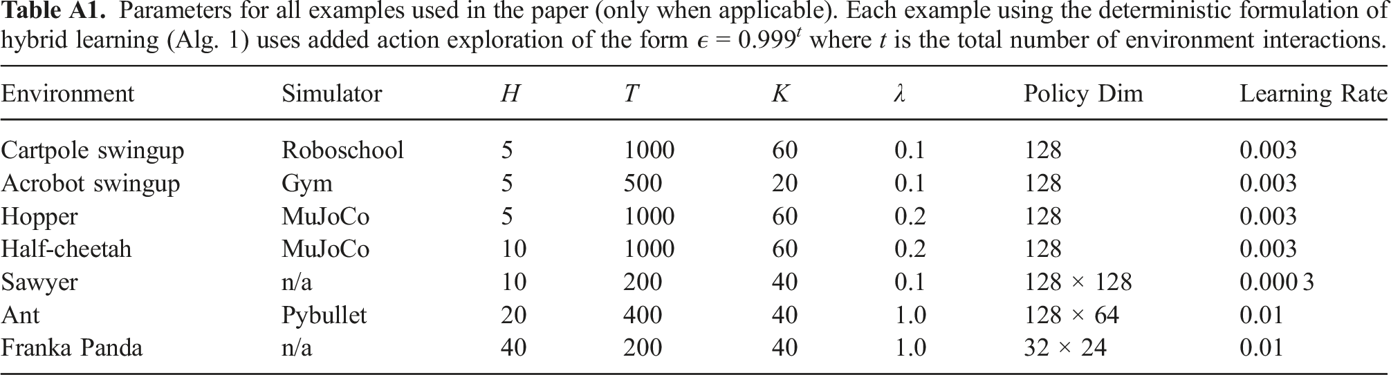
Environment
Simulator
H
T
K
λ
Policy Dim
Learning Rate
Cartpole swingup
Roboschool
5
1000
60
0.1
128
0.003
Acrobot swingup
Gym
5
500
20
0.1
128
0.003
Hopper
MuJoCo
5
1000
60
0.2
128
0.003
Half-cheetah
MuJoCo
10
1000
60
0.2
128
0.003
Sawyer
n/a
10
200
40
0.1
128 × 128
0.000 3
Ant
Pybullet
20
400
40
1.0
128 × 64
0.01
Franka Panda
n/a
40
200
40
1.0
32 × 24
0.01
The goal for both the cartpole swingup environment and the Acrobot swingup environment is to swing the pendulum up to the vertical position. We refer to both of these examples as “swingup tasks.” We chose these tasks to demonstrate the performance capabilities of the model-based method. Pendulum swingup tasks are well understood, low dimension, underactuated control problems for which we anticipated the model-based method would outperform the model-free method. Given enough samples, the model-free method should also be able to learn these tasks, but the model-free method would require many more samples to learn the task.
The goal for both the hopper environment and the half-cheetah environments is to learn a gait to move forward in a 2D environment as quickly as possible. We refer to both of these examples as “locomotion tasks.” We chose the two locomotion tasks to demonstrate the advantages of model-free methods. Model-free methods have been used to learn control tasks in high-dimensional spaces, so we anticipated the model-free method would outperform the model-based methods for the locomotion tasks.
Models: For each deterministic simulated benchmark example, we use a deterministic model-predictive controller (Ansari and Murphey, 2016) for the model-based method. For all other experiments, we use a neural-network based implementation of model-predictive path integral for reinforcement learning (Williams et al., 2017) for our model-based method.
For all model-based and hybrid learning simulated examples, the dynamics are represented by st+1 = s
t
+ f(s
t
, a
t
), where f(s
t
, a
t
) =
The reward function is modeled as a two layer network with 200 hidden nodes and the RELU activation function. Both the reward function and dynamics model are optimized using Kingma and Ba (2014) with learning rates specified in Table A1. The model is regularized using the negative log-loss of a normal distribution where the variance,
Policy: For the model-free and hybrid learning examples, we use Soft Actor-Critic (SAC) to update our model-free policy. We use the hyperparameters for SAC specified by the shared parameters in Haarnoja et al. (2018b) including the structure of the soft Q functions and automatic gradient-based temperature tuning method and excluding the batch size and policy. Instead, we match the batch size of 128 samples used with model learning and use a simpler policy representation. Our policy is parameterized by a normal distribution with a mean function defined as a single-layer network with the RELU nonlinearity and 128 hidden nodes. The diagonal of the variance is also specified using a single-layer network with 128 hidden nodes and the RELU nonlinearity. The parameters for SAC are held constant across all experiments to remove any impact of hyperparameter tuning.
The ant and Franka robot examples with behavior cloning use the policy structure defined in Table A1. The policy is structured similarly to the parameterization mentioned in the simulated benchmarks above. The negative log-loss of the normal distribution is used for behavior cloning expert demonstrations with a learning rate of 0.01 for each method.
Reward Function: We modified the Gym Acrobot environment (Brockman et al., 2016) to test in the continuous space and updated the reward function to include a dependency on the action and the state. The reward function is defined as
Robot Experiments: In all robot experiments, a camera is used to identify the location of objects in the environment using landmark tags and color image processing.
For the Sawyer robot example, the robot has no knowledge of the physical properties of the blocks (including size, weight, and material) or the true location of objects in the world. The state is comprised of the position of each of the six blocks in the workspace relative to the robot’s end-effector. The “target block” is always a fixed location in the state vector, but the five “clutter” blocks are sorted from closest to furthest from the end-effector to enable generalization. Without this sorting, the experimenter would also need to shuffle the “clutter” blocks around the “target” block, which would extend the testing duration.
The action space is the robot’s end-effector velocity.
The reward is defined as
where pee2t, pδt, and a are the pose of the target block relative to the end-effector, the change in target block position relative to the prior time step, and the control, respectively.
Each trial can be a maximum of 200 steps, but due to physical workspace constraints, we terminate the episode if the robot pushes the target block outside of the workspace. To account for this early termination, we post-processed the data to add a penalty proportional to the number of episode steps remaining when the block was pushed out of reach.
For the Franka robot, the state is defined as the end-effector position, the block position, and the gripper state (open or closed) as well as the measured wrench at the end-effector. The action space is defined as the commanded end-effector velocity. The reward function is defined as
where
Hybrid learning with behavior cloning
In this section, we extend to our hybrid learning approach to use expert demonstrations as experience. We use imitation learning, specifically behavior cloning, as an initialization for how a robot should accomplish a task. This approach wraps around either the deterministic and stochastic hybrid learning approaches presented in Section. We outline the algorithmic implementation hybrid learning with behavior cloning in Alg. 3.
Hybrid Learning with Behavior Cloning 1: Randomly initialize continuous differentiable models f(s, a), r(s, a) with parameters ψ and policy π(a | s) with parameter θ. Initialize memory buffer 2: ▷ get expert demonstrations 3: 4: observe state s
t
, expert action a
t
5: observe st+1, r
t
from environment 6: 7: 8: ▷ update models using data 9: update ψ using 10: update θ using ▷ test in environment 11: 12: observe state s
t
13: get action a
t
Alg. 1 or 2 14: observe st+1, r
t
from environment 15: 16: 17: if task not done, continue 18:
Related Work Implementation Details
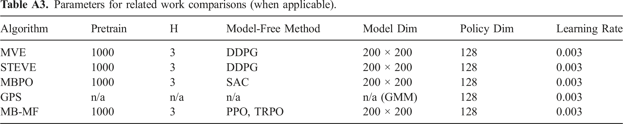
This section details the modifications made to related work implementations to compare to the hybrid results presented in this paper. Table A3 provides a list of the general hyperparameters used for each related work algorithm tested. Hyperparameters specific to each algorithm are specified below. Several algorithms assumed access to or learned a termination function. For these comparisons, we excluded the termination function from all implementations. Many of the comparison methods required pretraining their models, so we added 1000 steps of pretraining with random actions to our stochastic hybrid learning algorithm. We also increased the size of our neural network model to 2 layers for these comparisons. Each comparison algorithm is described below.
Model-Based Value Expansion (MVE): MVE uses only the model-free policy to interact with the environment. Experience is used to fit a dynamics model. During each update, the model is used to imagine future transitions for rollouts of fixed short duration horizons (H). These imagined transitions are incorporated into the Q-value target estimation (critic) update. The original implementation only learned a dynamics transition function and assumed access to a reward function and a termination function (Feinberg et al., 2018). We removed the termination function and added a learned reward function. Figure 9 shows the performance curves for hybrid learning and MVE. Pairwise comparison between our method and MVE. These are the same results presented in Figure 8. Note: Markers are included for distinguishing between methods only and do not represent all data points.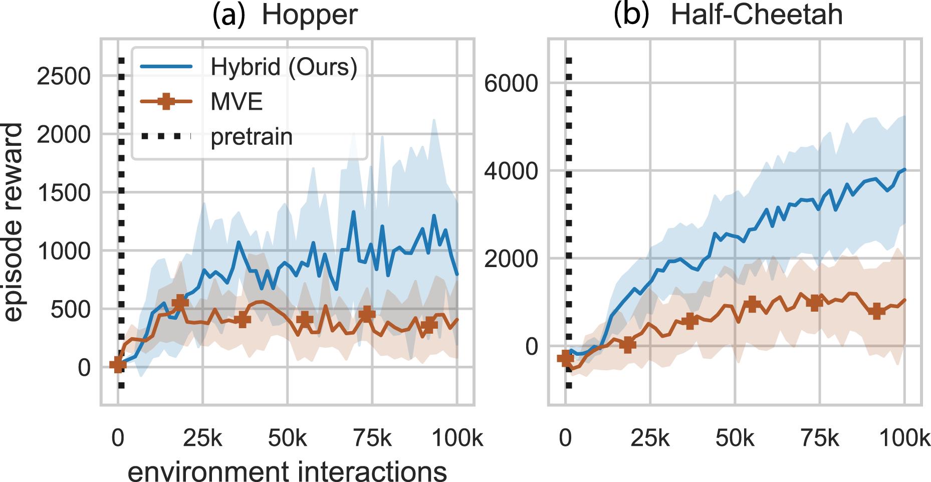
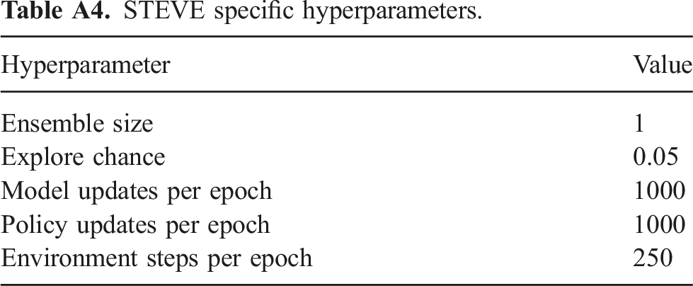
Stochastic Ensemble Value Expansion (STEVE): STEVE builds on MVE by performing rollouts on all horizon lengths between 0 and H. This algorithm additionally adds the ability to learn an ensemble of models. The original implementation learned a dynamics transition function, a reward function, and a termination function (Buckman et al., 2018). We removed the termination function and tested only a single model for these comparisons. Figure 10 shows the performance curves for hybrid learning and STEVE. Pairwise comparison between our method and STEVE. These are the same results presented in Figure 8. Note: Markers are included for distinguishing between methods only and do not represent all data points.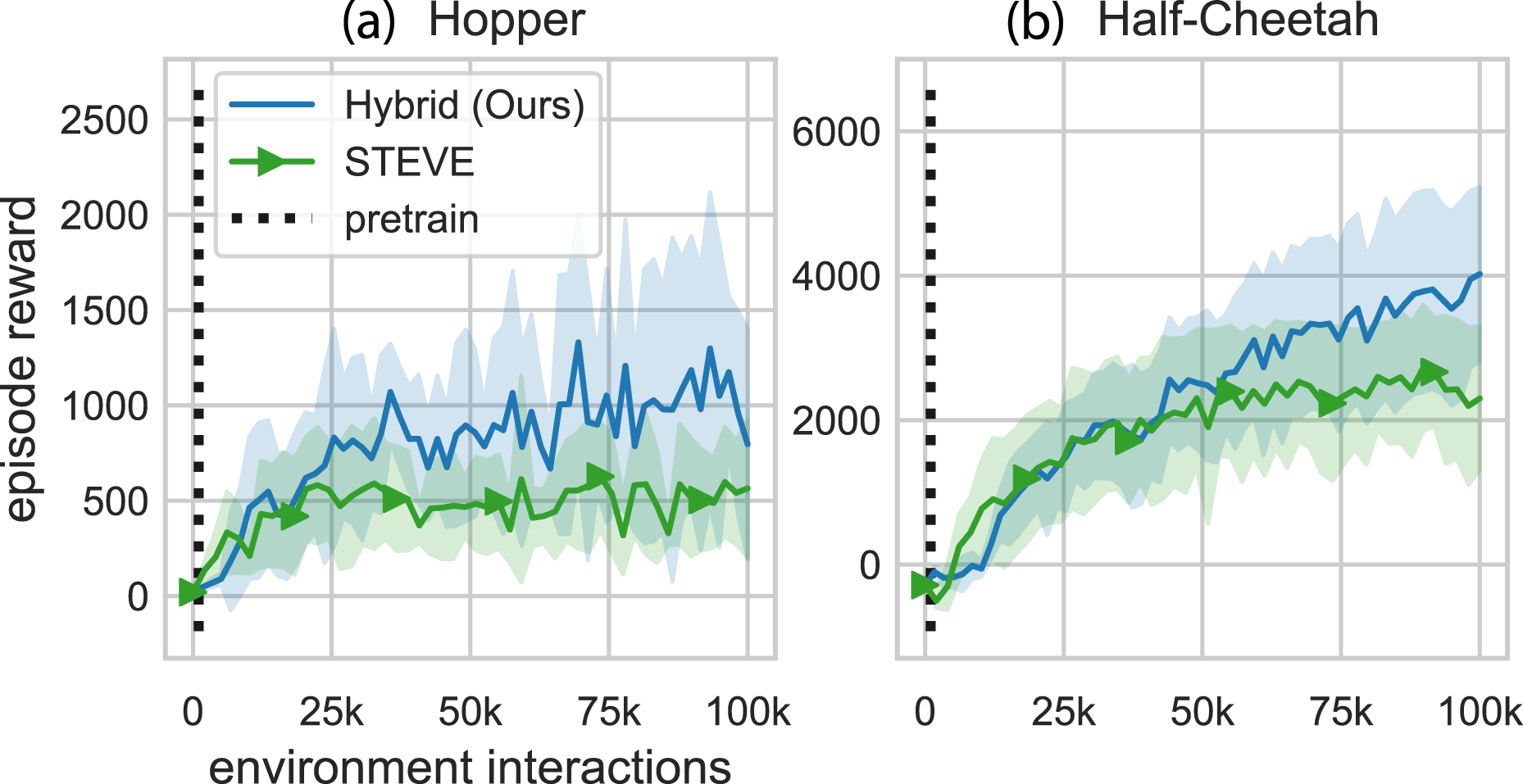
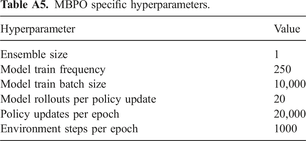
Model-Based Policy Optimization (MBPO): MBPO optimizes a policy under a learned model (Janner et al., 2019). Similar to MVE and STEVE, only the policy interacts with the environment and collects data. The original implementation assumed the termination function was known and used an ensemble of dynamics models. Additionally, the original implementation used all data collected from the environment to train the models during each model update iteration. We removed the termination function and tested only a single model for these comparisons. We also used a subset of the collected data for model updates. Figure 11 shows the performance curves for hybrid learning and MBPO. Pairwise comparison between our method and MBPO. These are the same results presented in Figure 8. Note: Markers are included for distinguishing between methods only and do not represent all data points.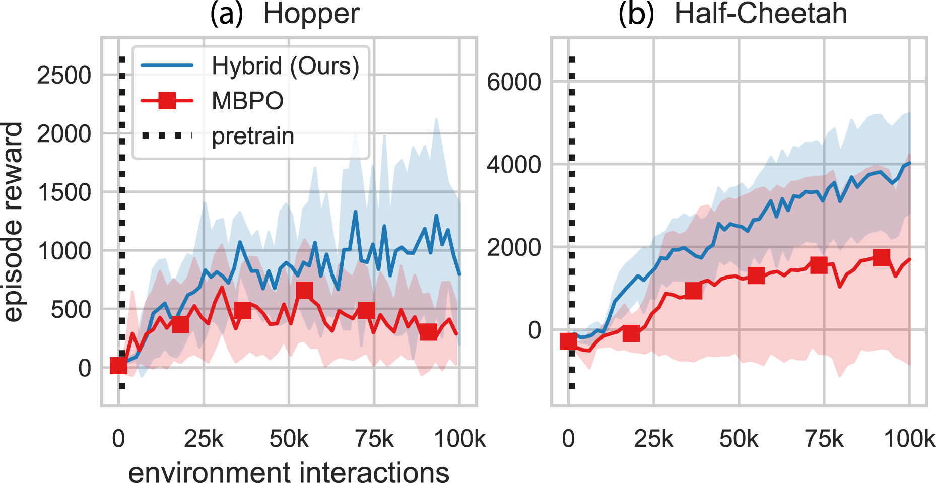
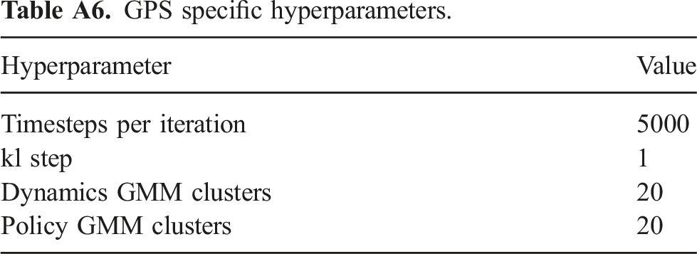
Guided Policy Search (GPS): GPS interacts with the environment via the model-based controller, rather than the model-free policy. The dynamics are modeled to be Gaussian-linear time varying and the reward function is assumed to be known. The dynamics are modeled as a Gaussian mixture model (GMM), and the algorithm assumes the reward function is known. The policy is trained via behavior cloning with constraints preventing the policy updates from deviating too far from the last implemented trajectory. The original implementations of GPS often used shorter horizon tasks than the full gym benchmarks, but we used the original length episodes for comparison purposes. We used the Mirror Descent variant of Guided Policy Search (MD-GPS) (Montgomery and Levine, 2016). Another difference between this simulation and the others is that it cannot handle true early termination due to the time varying controller. The gym hopper environment “ends” when the hopper falls out of a desired configuration. For GPS testing of the gym hopper environment, the “done” output is ignored and instead the “alive bonus” (typically one in the gym environment) is toggled to zero when done is called by the simulator. Figure 12 shows the performance curves for hybrid learning and GPS. Pairwise comparison between our method and GPS. These are the same results presented in Figure 8. Note: Markers are included for distinguishing between methods only and do not represent all data points.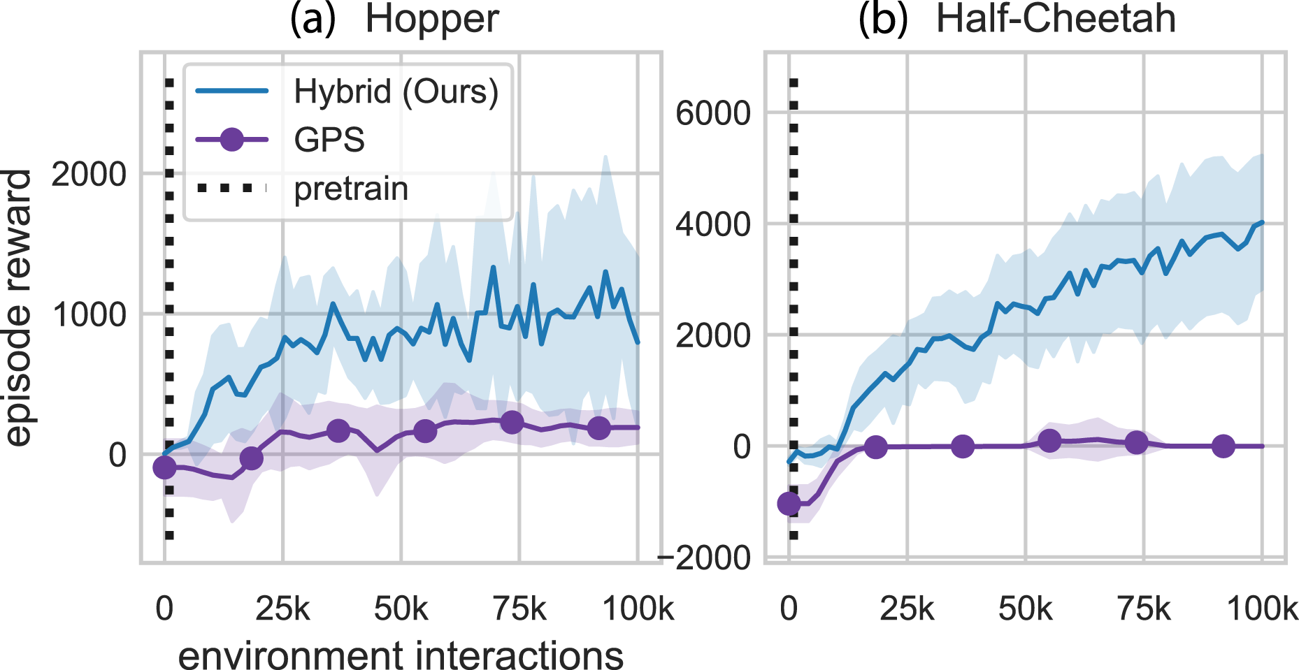
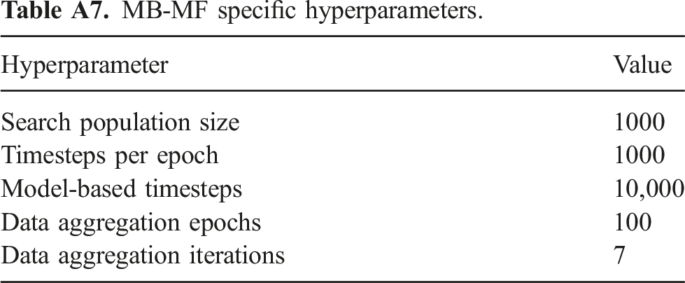
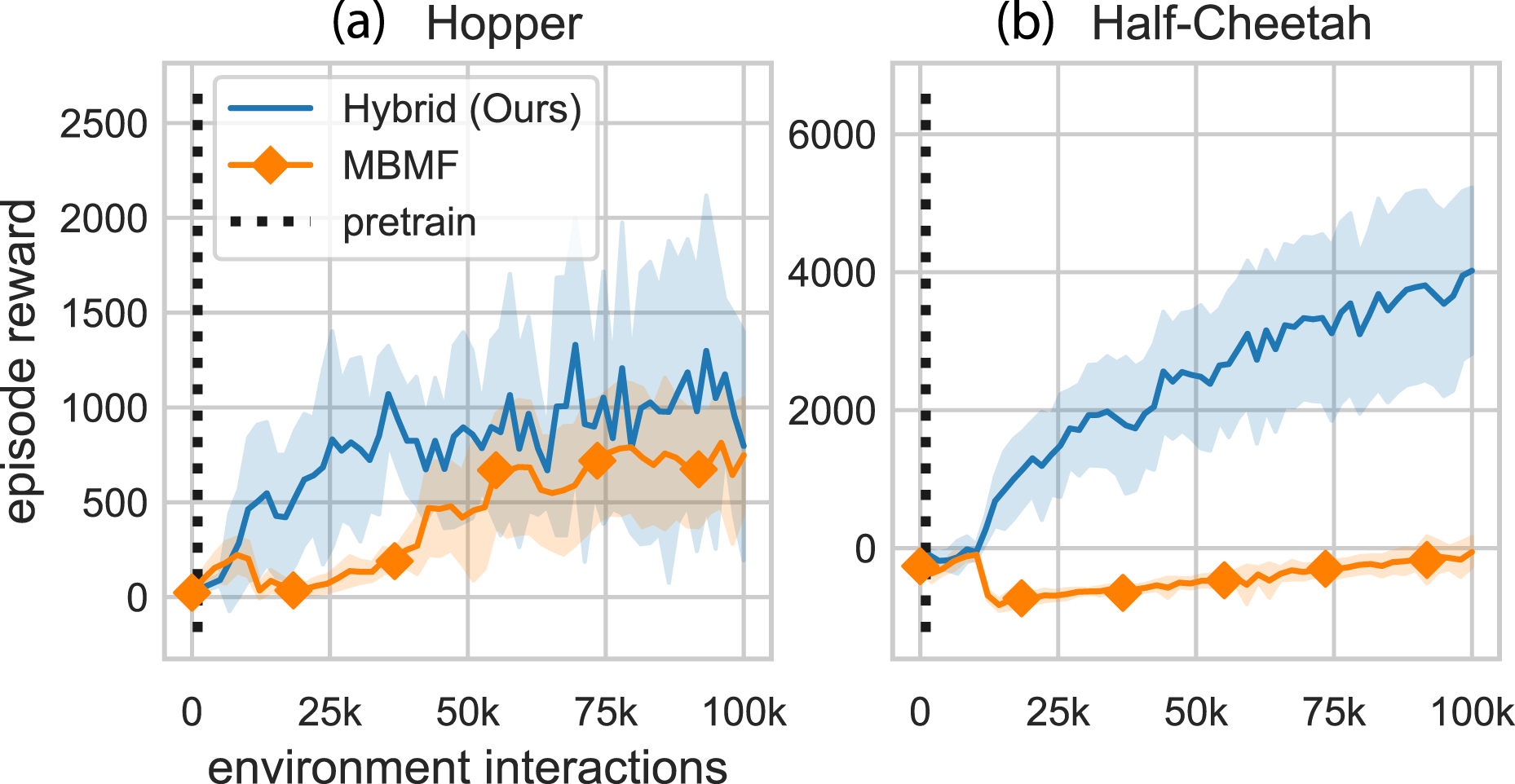
Mode-Free Model-Based (MB-MF): MB-MF uses a multi-stage approach (Nagabandi et al., 2018). First, a controller is learned using a random shooting method. Then the controller is transferred to a model-free policy using data aggregation. Finally, the policy is fine-tuned using a model-free method. The original method presented in the paper was able to fully observe all environment states, but the version implemented here only had access to the default gym environment (partially observable) state. Figure 13 shows the performance curves for hybrid learning and MB-MF. MVE specific hyperparameters. Parameters for related work comparisons (when applicable). STEVE specific hyperparameters. MBPO specific hyperparameters. GPS specific hyperparameters. MB-MF specific hyperparameters. Pairwise comparison between our method and MB-MF. These are the same results presented in Figure 8. Note: Markers are included for distinguishing between methods only and do not represent all data points.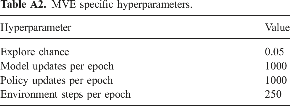
Hyperparameter
Value
Explore chance
0.05
Model updates per epoch
1000
Policy updates per epoch
1000
Environment steps per epoch
250
Algorithm
Pretrain
H
Model-Free Method
Model Dim
Policy Dim
Learning Rate
MVE
1000
3
DDPG
200 × 200
128
0.003
STEVE
1000
3
DDPG
200 × 200
128
0.003
MBPO
1000
3
SAC
200 × 200
128
0.003
GPS
n/a
n/a
n/a
n/a (GMM)
128
0.003
MB-MF
1000
3
PPO, TRPO
200 × 200
128
0.003
Hyperparameter
Value
Ensemble size
1
Explore chance
0.05
Model updates per epoch
1000
Policy updates per epoch
1000
Environment steps per epoch
250
Hyperparameter
Value
Ensemble size
1
Model train frequency
250
Model train batch size
10,000
Model rollouts per policy update
20
Policy updates per epoch
20,000
Environment steps per epoch
1000
Hyperparameter
Value
Timesteps per iteration
5000
kl step
1
Dynamics GMM clusters
20
Policy GMM clusters
20
Hyperparameter
Value
Search population size
1000
Timesteps per epoch
1000
Model-based timesteps
10,000
Data aggregation epochs
100
Data aggregation iterations
7
References
Supplementary Material
Please find the following supplemental material available below.
For Open Access articles published under a Creative Commons License, all supplemental material carries the same license as the article it is associated with.
For non-Open Access articles published, all supplemental material carries a non-exclusive license, and permission requests for re-use of supplemental material or any part of supplemental material shall be sent directly to the copyright owner as specified in the copyright notice associated with the article.