RadarSLAM: A robust simultaneous localization and mapping system for all weather conditions

Abstract

A Simultaneous Localization and Mapping (SLAM) system must be robust to support long-term mobile vehicle and robot applications. However, camera and LiDAR based SLAM systems can be fragile when facing challenging illumination or weather conditions which degrade the utility of imagery and point cloud data. Radar, whose operating electromagnetic spectrum is less affected by environmental changes, is promising although its distinct sensor model and noise characteristics bring open challenges when being exploited for SLAM. This paper studies the use of a Frequency Modulated Continuous Wave radar for SLAM in large-scale outdoor environments. We propose a full radar SLAM system, including a novel radar motion estimation algorithm that leverages radar geometry for reliable feature tracking. It also optimally compensates motion distortion and estimates pose by joint optimization. Its loop closure component is designed to be simple yet efficient for radar imagery by capturing and exploiting structural information of the surrounding environment. Extensive experiments on three public radar datasets, ranging from city streets and residential areas to countryside and highways, show competitive accuracy and reliability performance of the proposed radar SLAM system compared to the state-of-the-art LiDAR, vision and radar methods. The results show that our system is technically viable in achieving reliable SLAM in extreme weather conditions on the RADIATE Dataset, for example, heavy snow and dense fog, demonstrating the promising potential of using radar for all-weather localization and mapping.

1. Introduction

Simultaneous Localization and Mapping (SLAM) has attracted substantial interest over recent decades, and extraordinary progress has been made in the last 10 years in both the robotics and computer vision communities. In particular, camera and LiDAR based SLAM algorithms have been extensively investigated (Engel et al. (2014), Mur-Artal et al. (2015), Zhang and Singh (2014), Shan and Englot (2018)) and progressively applied to various real-world applications. Their robustness and accuracy are also improved further by fusing with other sensing modalities, especially Inertial Measurement Unit (IMU) based motion as a prior (Qin et al. (2018), Campos et al. (2020), Shan et al. (2020)).

Most existing camera and LiDAR sensors fundamentally operate within or near-visible electromagnetic spectra, which means that they are more susceptible to illumination changes, floating particles and water drops in the environments. It is well-known that vision suffers from low illumination, causing image degradation with dramatically increased motion blur, pixel noise and texture losses. The quality of LiDAR point clouds and camera images can also degenerate significantly, for instance, when facing a realistic density of fog particles, raindrops and snowflakes in mist, rain and snow. Studies of the degradation of LiDAR sensors are performed in (Jokela et al. (2019); Carballo et al. (2020)) and suggest that the data of all the tested LiDAR sensors degrades, to some extent, in foggy, rainy and snowy conditions. Given the fact that a motion prior is mainly effective in addressing short-period and temporary sensor degradation, even visual-inertial or LiDAR-inertial SLAM systems are anticipated to fail in these challenging weather conditions.

Radar is a type of active sensor, whose electromagnetic spectrum usually lies in a much lower frequency (GHz) band than camera and LiDAR (from THz to PHz). Therefore, it can operate more reliably in the majority of weather and light conditions. It also has additional benefits, for example, further sensing range, relative velocity estimates from the Doppler effect and absolute range measurement. Recently, radar has been gradually considered to be indispensable for safe autonomy and has been increasingly adopted in the automotive industry for obstacle detection and Advanced Driver-Assistance Systems (ADAS). Meanwhile, recent advances in Frequency-Modulated Continuous-Wave (FMCW) radar systems make radar sensing more appealing since it is able to provide a relatively dense representation of the environment, instead of only returning sparse detections. With these advancements in radar sensing, radar-based SLAM system can be deployed on various platforms and in different environments, for example, surface mining, underground mining, off-road driving.

However, radar has a distinct sensor model and its data is formed very differently from vision and LiDAR. There are different challenges for radar-based SLAM compared to vision and LiDAR based SLAM. For example, its noise and clutter characteristics are complex, for example, electromagnetic radiation in the atmosphere and multi-path reflection, and its noise level tends to be much higher. This means that existing feature extraction and matching algorithms may not be well suited for radar images. Unlike LiDAR sensors, most FMCW radars do not provide 3D elevation information.

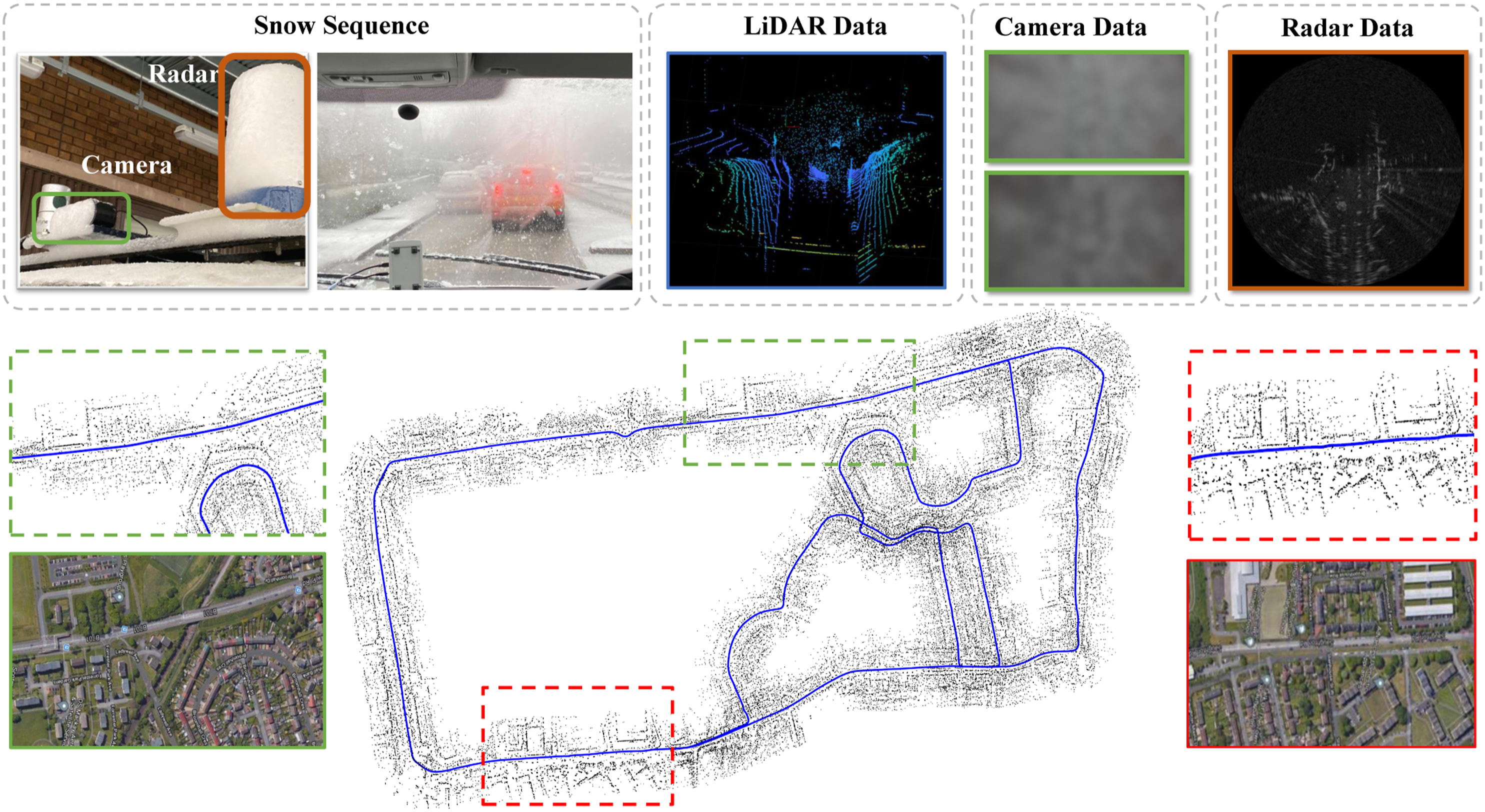
In this paper, we propose a novel SLAM system based on a FMCW radar. It can operate in various outdoor scenarios, for example, busy city streets and highways, and weather conditions, for example, heavy snowfall and dense fog, see Figure 1. Our main contributions are:

• A robust data association and outlier rejection mechanism for radar-based feature tracking by leveraging radar geometry.

• A novel motion compensation model formulated to reduce motion distortion induced by a low scanning rate. The motion compensation is jointly optimized with pose estimation in an optimization framework.

• A fast and effective loop closure detection scheme designed for a FMCW radar with dense returns.

• Extensive experiments on three available public radar datasets, demonstrating and validating the feasibility of a SLAM system operating in extreme weather conditions.

• Unique robustness and minimal parameter tuning, that is, the proposed radar SLAM system is the only competing method which can work properly on all data sequences, in particular using an identical set of parameters without much parameter tuning.

Figure 1.

Map and trajectory estimated by our proposed radar SLAM system on a self-collected Snow Sequence. We can observe random noisy LiDAR points around the vehicle due to reflection from snowflakes. The camera is completely covered by frozen snow. The magnified areas are compared with satellite images from Google Maps showing reconstructed buildings and roads. Our proposed radar SLAM method can successfully handle this challenging sequence with heavy snowfall.

The rest of the paper is structured as follows. In Sec. 2, we discuss related work. In Sec. 3, we elaborate on the geometry of radar sensing and the challenges of using radar for SLAM. The proposed motion compensation tracking model is presented in Sec. 4, followed by the loop closure detection and pose graph optimization in Sec. 5. Experiments, results and system parameters are presented in Sec. 6. Finally, the conclusions and future work are discussed in Sec. 7.

2. Related work

In this section, we discuss related work on localization and mapping in extreme weather conditions using optical sensor modalities, that is, camera and LiDAR. We also review the past and current state-of-the-art radar-based localization and mapping methods.

2.1. Vision and LiDAR based localization and mapping in adverse weathers

Typical adverse weather conditions include rain, fog and snow which usually cause degradation in image quality or produce undesired effects, for example, due to rain streaks or ice. Therefore, significant efforts have been made to alleviate this impact by pre-processing image sequences to remove the effects of rain (Garg and Nayar (2004)), (Ren et al. (2017)), for example using a model based on matrix decomposition to remove the effects of both snow and rain in the latter case. In contrast, (Li et al. (2016)) removes the effects of rain streaks from a single image by learning the static and dynamic background using a Gaussian Mixture Model. A de-noising generator that can remove noise and artefacts induced by the presence of adherent rain droplets and streaks is trained in (Porav et al. (2019)) using data from a stereo rig. A rain mask generated by temporal content alignment of multiple images is also used for keypoint detection (Huang et al. (2019); Yamada et al. (2019)). In spite of these pre-processing strategies, existing visual SLAM and visual odometry (VO) methods tend to be susceptible to these image degradations and tend to perform poorly under such condition.

The quality of LiDAR scans can also be degraded when facing rain droplets, snowflakes and fog particles in extreme weather. A filtering based approach is proposed in (Charron et al. (2018)) to de-noise 3D point cloud scans corrupted by snow before using them for localization and mapping. To mitigate the noisy effects of LiDAR reflection from random rain droplets, (Zhang et al. (2018)) proposes ground-reflectivity and vertical features to build a prior tile map, which is used for localization in a rainy weather. In contrast to process 3D LiDAR scans, (Aldibaja et al. (2016)) suggests the use of 2D LiDAR images reconstructed and smoothed by Principal Component Analysis (PCA). An edge-profile matching algorithm is then used to match the run time LiDAR images with a mapped set of LiDAR images for localization. However, these methods are not reliable when the rain, snow or fog is moderate or heavy. The results of LIO-SAM (Shan et al. (2020)), a LiDAR based odometry and mapping algorithm fused with IMU data, in light snow show that a LiDAR based approach can work to some degree in snow. However, as the snow increases, the reconstructed 3D point cloud map is corrupted to a high degree with random points from the reflection of snowflakes, which reduces the map’s quality and its re-usability for localization.

In summary, camera and LiDAR sensors are naturally sensitive to rain, fog and snow. Therefore, attempts to use these sensors to perform localization and mapping tasks in adverse weather are limited.

2.2. Radar-based localization and mapping

Using Millimetre Wave (MMW) radar as a guidance sensor for autonomous vehicle navigation can be traced back two or three decades. An Extended Kalman Filter (EKF) based beacon localization system is proposed by (Clark and Durrant-Whyte (1998)) where the wheel encoder information is fused with range and bearing obtained by radar. One of the first substantial solutions for MMW radar-based SLAM is proposed in (Dissanayake et al. (2001)), detecting features and landmarks from radar to provide range and bearing information. (Jose and Adams (2005)) further extends the landmark description and formalizes an augmented state vector containing rich absorption and localization information about targets. A prediction model is formed for the augmented SLAM state. Instead of using the whole radar measurement stream to perform scan matching, (Chandran and Newman (2006)) suggests treating the measurement sequence as a continuous signal and proposes a metric to assess the quality of map and estimate the motion by maximizing the map quality. A consistent map is built using a FMCW radar, an odometer and a gyroscope (Rouveure et al. (2009)). Specifically, vehicle motion is corrected using an odometer and a gyrometer while the map is updated by registering radar scans. Instead of extracting and registering feature points, (Checchin et al. (2010)) uses the Fourier-Mellin Transform (FMT) to estimate the relative transformation between two radar images. In (Vivet et al. (2013)), two approaches are evaluated for localization and mapping in a semi-natural environment using only a radar. The first one is the aforementioned FMT computing relative transformation from whole images, while the second one uses a velocity prior to correct a distorted scan (Vivet et al. (2012)). However, both methods are evaluated without any loop closure detection. A landmark based pose graph radar SLAM system proves that it can work in dynamic environments (Schuster et al. (2016)). (Marck et al. (2013)) use an Iterative Closest Point algorithm (ICP) to register the returned radar point cloud and a Particle filter to map the indoor environment. (Park et al. (2019)) studies the localization to a prior LiDAR map using radar in a low visibility situation. A low-cost millimetre-wave radar is used to provide robust ego-motion estimation in indoor environments in (Almalioglu et al. (2021)) with a RNN-based motion model.

Recently, FMCW radar sensors have been increasingly adopted for vehicles and autonomous robots. (Cen and Newman (2018)) extract meaningful landmarks for robust radar scan matching, demonstrating the potential of using radar to provide odometry information for mobile vehicles in dynamic city environments. This work is extended with a graph based matching algorithm for data association (Cen and Newman (2019)). Radar odometry might fail in challenging environments, such as a road with hedgerows on both sides. Therefore, (Aldera et al. (2019b)) train a classifier to detect failures in the radar odometry using inertial measurements as supervision to automatically label good and bad odometry estimation. Recently, a direct radar odometry method has been proposed to estimate relative pose using FMT, with local graph optimization to further boost the performance ((Park et al. (2020)). In (Burnett et al. (2021)), they study the necessity of motion compensation and Doppler effects on the recent emerging spinning radar for urban navigation.

Deep Learning based radar odometry and localization approaches have been explored in (Barnes et al. (2020b), Aldera et al. (2019a), Barnes and Posner (2020), Gadd et al. (2020), De Martini et al. (2020), Gadd et al. (2021), Tang et al. (2020a,b), Săftescu et al. (2020), Wang et al. (2021)). Specifically, in (Aldera et al. (2019a)) the coherence of multiple measurements is learnt to decide which information should be kept in the readings. In (Barnes et al. (2020b)), a mask is trained to filter out the noise from radar data and Fast Fourier Transform (FFT) cross correlation is applied to the masked images to compute the relative transformation. The experimental results show impressive accuracy of odometry using radar. A self-supervised framework is also proposed for robust keypoint detection on Cartesian radar images which are further used for both motion estimation and loop closure detection (Barnes and Posner (2020)). A hierarchical approach to place recognition and pose refinement for FMCW radar localization is presented in (De Martini et al. (2020)) with compelling performance by using one experience. Promising result for radar based place recognition is shown in (Gadd et al. (2021)) by learning and embedding from sequences in an unsupervised manner.

Full radar-based SLAM systems are able to reduce drift and generate a more consistent map once a loop is closed. A real-time pose graph SLAM system is proposed in (Holder et al. (2019)), which extracts keypoints and computes the GLARE descriptor (Himstedt et al. (2014)) to identify loop closure. However, the system depends on other sensory information, for example, rear wheel speed, yaw rates and steering wheel angles.

2.2.1. Adverse weather

Although radar is considered more robust in adverse weather, the aforementioned methods do not directly demonstrate its operation in these conditions. (Yoneda et al. (2018)) proposes a radar and GNSS/IMU fused localization system by matching query radar images with mapped ones, and tests radar-based localization in three different snow conditions: without snow, partially covered by snow and fully covered by snow. It shows that the localization error grows as the volume of snow increases. However, they did not evaluate their system during snow but only afterwards. To explore the full potential of FMCW radar in all weathers, our previous work (Hong et al. (2020)) proposes a feature matching based radar SLAM system and performs experiments in adverse weather conditions without the aid of other sensors. It demonstrates that radar-based SLAM is capable of operating even in heavy snow when LiDAR and camera both fail. In other interesting recent work, ground penetrating radar is used for localization in inclement weather (Ort et al. (2020)) This takes a completely different perspective to address the problem. The ground penetrating radar (GPR) is utilized for extracting stable features beneath the ground. During the localization stage, the vehicle needs an IMU, a wheel encoder and GPR information to localize.

In this work, we extend our preliminary results presented in (Hong et al. (2020)) with a novel motion estimation algorithm optimally compensating motion distortion and an improved loop closure detection. We also carry out extensive additional experiments, demonstrating more tests and results of Radar SLAM system operating in various weather conditions, including the MulRan dataset and more sequences in adverse weather conditions.

3. Radar sensing and system overview

In this section, we describe the working principle of a FMCW radar and its sensor model. We also elaborate the challenges of employing a FMCW radar for localization and mapping.

3.1. Notation

Throughout this paper, a reference frame j is denoted as ${\mathrm{ℱ}}_j$ and a homogeneous coordinate of a 2D point ${\mathcal{F}}_j$ in frame ${\mathrm{ℱ}}_j$ is defined as ${\mathbf{p}}_j={\left[x_j,y_j,1\right]}^{\mathrm{\top }}$ . A homogeneous transformation T _i , _j ∈ SE (2) which transforms a point from the coordinate frame ${\mathrm{ℱ}}_j$ to ${\mathrm{ℱ}}_i$ is denoted by a transformation matrix

${\mathbf{T}}_{i,j}=\left[\begin{array}{cc}{\mathbf{R}}_{i,j}& {\mathbf{t}}_{i,j}\\ \mathbf{0}& 1\end{array}\right]$

(1)

where R _i , _j ∈ SO(2) is the rotation matrix and ${\mathbf{t}}_{i,j}\in {ℝ}^2$ is the translation vector. Perturbation $\omega \in {ℝ}^3$ around the pose T _i , _j uses a minimal representation and its Lie algebra representation is expressed as ${\omega }^{\wedge }\in \text{se}\left(2\right)$ . We use the left multiplication convention to define its increment on T _i , _j with an operator ⊕, that is

$\omega \oplus {\mathbf{T}}_{i,j}=\exp \left({\omega }^{\wedge }\right)\cdot {\mathbf{T}}_{i,j}$

(2)

A polar radar image and its bilinear interpolated Cartesian counterpart are denoted as S and I, respectively. A point in the Cartesian image I is represented by its pixel coordinates P = [u,v]^⊤.

3.2. Geometry of a rotating frequency-modulated continuous-wave radar

There are two types of continuous-wave radar: unmodulated and frequency-modulated radars. Unmodulated continuous-wave radar can only measure the relative velocity of targeted objects using the Doppler effect, while a FMCW radar is also able to measure distances by detecting time shifts and/or frequency shifts between the transmitted and received signals. Some recently developed FMCW radars make use of multiple consecutive observations to calculate targets’ speeds so that Doppler processing is strictly required. This improves the processing performance and accuracy of target range measurements.

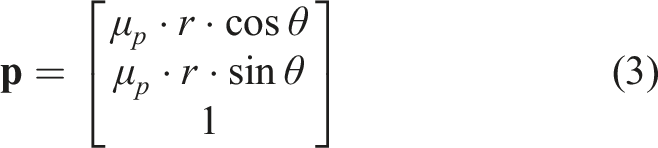
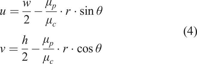
Assume a radar sensor rotates 360° clockwise in a full cycle with a total of N _s azimuth angles as shown in Figure 2(a), that is, the step size of the azimuth angle is 2π/N _s . For each azimuth angle, the radar emits a beam and collapses the return signal to the point where a target is sensed along a range without considering elevation. Therefore, a radar image is able to provide absolute metric information of distance, different from a camera image which lacks depth by nature. As shown in Figure 2(b), given a point (a, r) in a polar image S where a and r denote its azimuth and range, its homogeneous coordinates p can be computed by

$\mathbf{p}=\left[\begin{array}{c}{\mu }_p\cdot r\cdot \cos \theta \\ {\mu }_p\cdot r\cdot \sin \theta \\ 1\end{array}\right]$

(3)

where θ = − a ⋅ 2π/N _s is the ranging angle in Cartesian coordinates, and μ _p (m/pixel) is the scaling factor between the image space and the world metric space. This point on the polar image can also be related to a point on the Cartesian image I with a pixel coordinate P by

$\begin{array}{l}u=\frac{w}{2}-\frac{{\mu }_p}{{\mu }_c}\cdot r\cdot \sin \theta \hfill \\ v=\frac{h}{2}-\frac{{\mu }_p}{{\mu }_c}\cdot r\cdot \cos \theta \hfill \end{array}$

(4)

where w and h are the width and height of the Cartesian image, and μ _c (m/pixel) is the scale factor between the pixel space and the world metric space used in the Cartesian image. Therefore, the raw polar scan S can be transformed into a Cartesian space, represented by a grey-scale Cartesian image I through bilinear interpolation, as shown in Figure 2(b).

Figure 2.

Radar sensing and radar image formation. (a): A radar sends a beam with certain azimuth and elevation beamwidths, and the receiver waits for echoes from the target objects. Elevation information, like object height, is usually not retained and collapsed to one point of 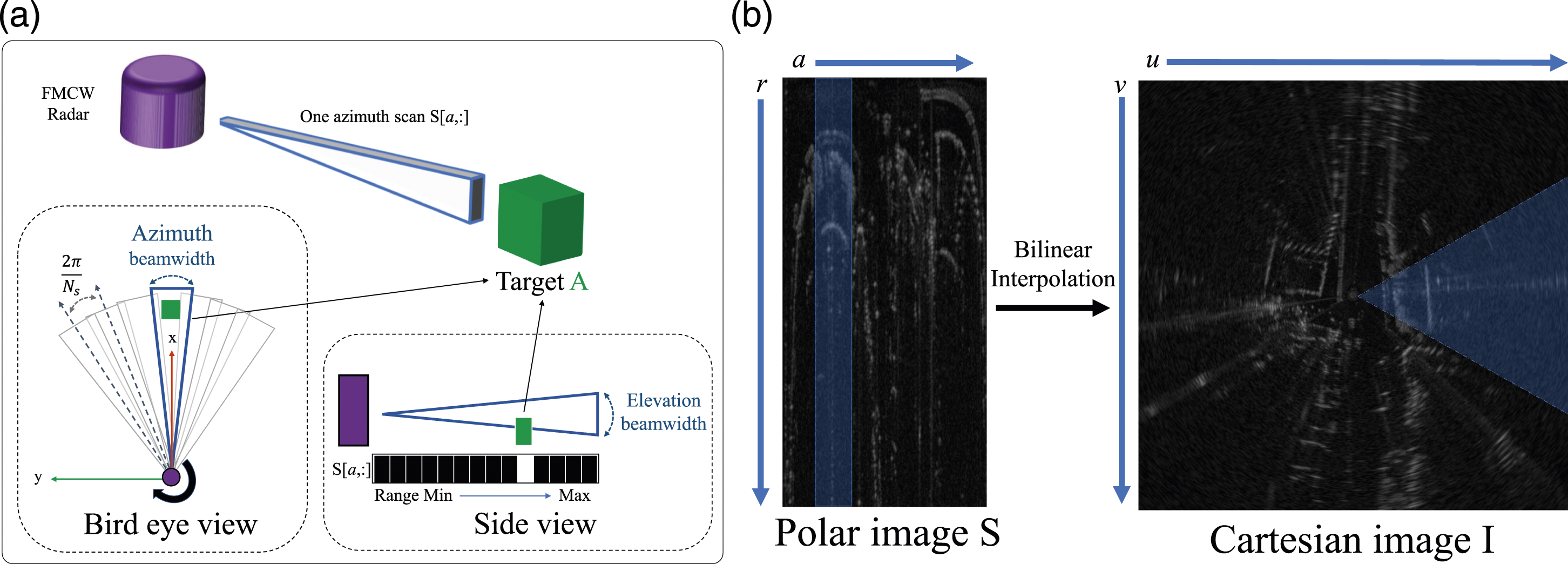S [a,:]. (b): Bilinear interpolation from a polar scan to a Cartesian image.

3.3. Challenges of radar sensing for simultaneous localization and mapping

Despite the increasingly widespread adoption of radar systems for perception in autonomous robots and in Advanced Driver-Assistance Systems (ADAS), there are still significant challenges for an effective radar SLAM system.

3.3.1. Coupled artefacts

As a radioactive sensor, radar suffers from multiple sources of artefacts and clutters, for example, speckle noise, receiver saturation and multi-path reflection, as shown in Figure 3(a). Speckle noise is the product of interaction between different radar waves which introduces light and dark random noisy pixels on the image. Meanwhile, multi-path reflection may create ‘ghost’ objects, presenting repetitive similar patterns on the image. The interaction of these multiple sources adds another dimension of complexity and difficulty when applying traditional vision based SLAM techniques to radar sensing.

Figure 3.

Three major types of challenges for radar SLAM.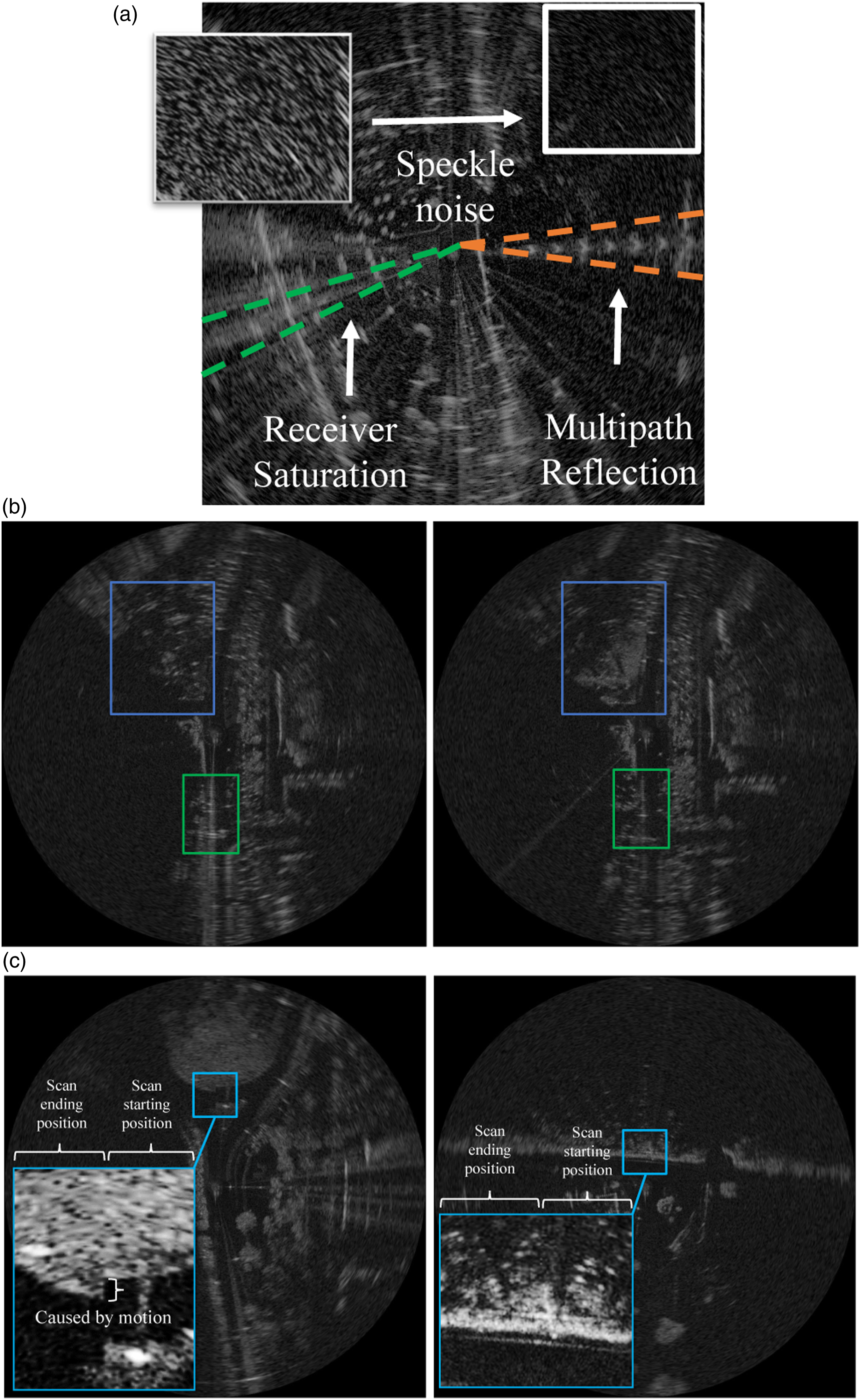

3.3.2. Discontinuities of detection

Radar operates at a longer wavelength than LiDAR, offering the advantage of perceiving beyond the closest object on a line of sight. However, this could become problematic for some key tasks in pose estimation, for example, frame-to-frame feature matching and tracking, since objects or clutter detected (not detected) in the current radar frame might suddenly disappear (appear) in next frame. As shown in Figure 3(b), this can happen even during a small positional change. This discontinuity of detection can introduce ambiguities and challenges for SLAM, reducing robustness and accuracy of motion estimation and loop closure.

3.3.3. Motion distortion

In contrast to camera and LiDAR, current mechanical scanning radar operates at a relatively low frame rate (4 Hz for our radar sensor). Within a full 360-degree radar scan, a high-speed vehicle can travel several metres and degrees, causing serious motion distortion and discontinuities on radar images, in particular between scans at 0 and 360°. An example in Figure 3(c) shows this issue on the Cartesian image on the left, that is, skewed radar detections due to motion distortion. By contrast, there are no skewed detections when it is static. Therefore, directly using these distorted Cartesian images for geometry estimation and mapping can introduce errors.

3.4. System overview

Having these challenges in mind, we propose a novel radar SLAM system which includes motion compensated radar motion estimation, loop closure detection and pose graph optimization. The system, shown in Figure 4, is divided into two threads. The main thread is the tracking thread which takes the Cartesian images as input, tracks the radar motion and creates new points and keyframes for mapping. The other parallel thread takes the polar images as input and is responsible for generation of the dense point cloud and computation of descriptors for loop closure detection. Finally, once a loop is detected, it performs pose graph optimization to correct the drift induced by tracking before updating the map.

Figure 4.

System diagram.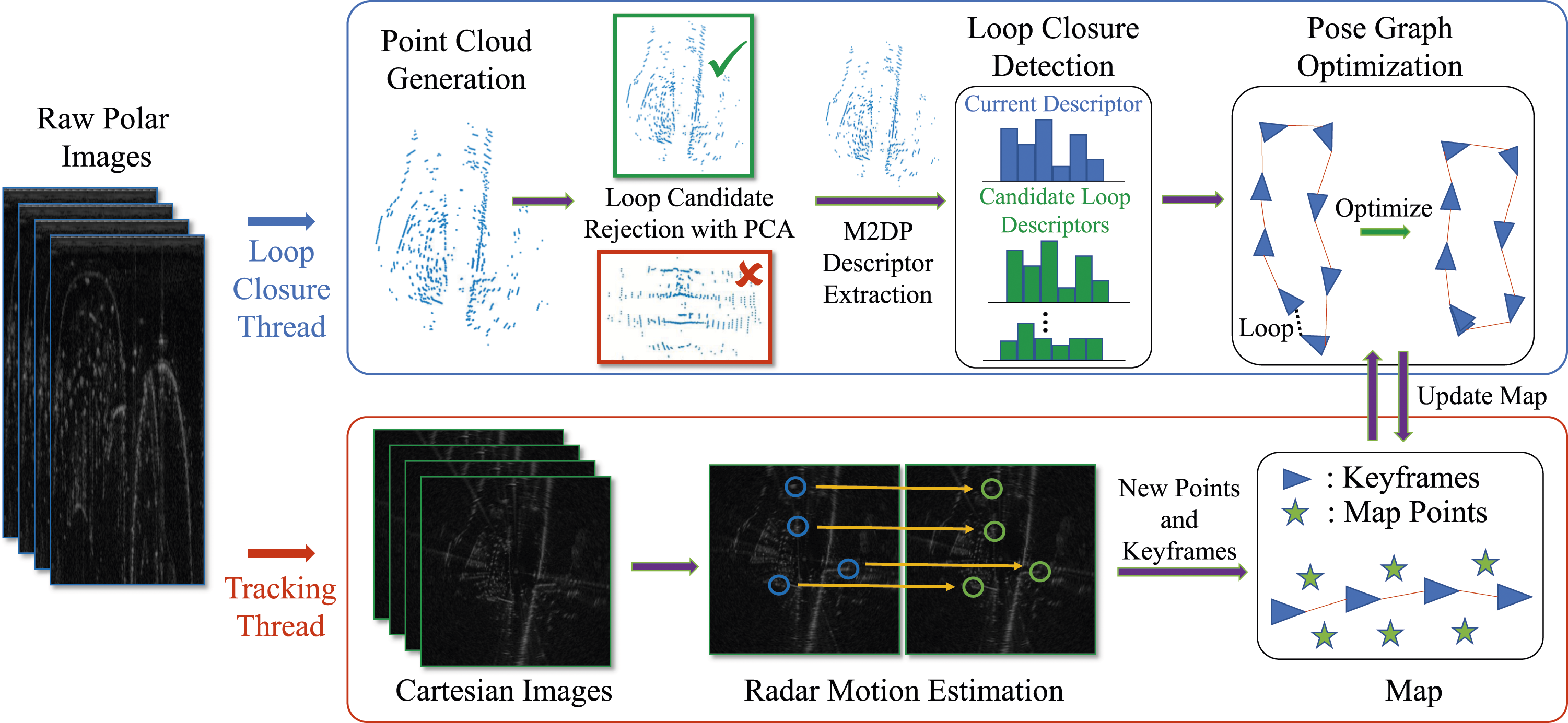

4. Radar motion estimation

This section describes the proposed radar motion estimation algorithm, which includes feature detection and tracking, graph based outlier rejection and radar pose tracking with optimal motion distortion compensation.

4.1. Feature detection and tracking

For each radar Cartesian image I _j , we first detect keypoints purely using a blob detector based on a Hessian matrix. Keypoints with Hessian responses larger than a threshold are selected as candidate points. The candidate points are then selected based on the adaptive non-maximal suppression (ANMS) algorithm (Bailo et al. (2018)), which selects points that are homogeneously spatially distributed. Instead of using a descriptor to match keypoints as in (Hong et al. (2020)), we track them between frames I_j−1 and I _j using the KLT tracker (Lucas and Kanade (1981)).

4.2. Graph based outlier rejection

It is inevitable that some keypoints are detected and tracked on dynamic objects, for example, cars, cyclists and pedestrians, and on radar noise, for example, multi-path reflection. We leverage the absolute metrics that radar images directly provide to form geometric constraints used for detecting and removing these outliers.

We apply a graph based outlier rejection algorithm described in (Howard (2008)). We impose a pairwise geometric consistency constraint on the tracked keypoint pair based on the fact that they should follow a similar motion tendency. The assumption is that most of the tracked points are from static scene data. Therefore, for any two pairs of keypoint matches between the current I _j and the last I_j−1 radar frames, they should satisfy the following pairwise constraint:

$\left|{\Vert {\mathbf{P}}_{j-1}^m-{\mathbf{P}}_{j-1}^n\Vert }_2-{\Vert {\mathbf{P}}_j^m-{\mathbf{P}}_j^n\Vert }_2\right|<{\delta }_c$

(5)

where $|\cdot |$ is the absolute operation, ‖⋅‖₂ is the Euclidean distance, δ _c is a small distance threshold, and ${\mathbf{P}}_{j-1}^m$ , ${\mathbf{P}}_{j-1}^n$ , ${\mathbf{P}}_j^m$ and ${\mathbf{P}}_j^n$ are the pixel coordinates of two pairs of tracked points between I_j−1 and I _j . Hence, ${\mathbf{P}}_{j-1}^m$ and ${\mathbf{P}}_j^m$ denote a pair of associated points while ${\mathbf{P}}_{j-1}^n$ and ${\mathbf{P}}_j^n$ is another pair, see Figure 5 for an intuitive example. A consistency matrix G is then used to represent all the associations that satisfy this pairwise consistency. If a pair of associations satisfies this constraint, the corresponding entry in G is set as one shown in Figure 5. Finding the maximum inlier set of all matches that are mutually consistent is equivalent to deriving the maximum clique of a graph represented by G, which can be solved efficiently using (Konc and Janezic (2007)). Once the maximum inlier set is obtained, it is used to compute the relative transformation T_j−1, j, which transforms a point from local frame j to local frame j − 1 using Singular Value Decomposition (SVD) (Challis (1995)). Given T_j−1, j and the fixed radar frame rate, an initial guess of current velocity ${\mathbf{v}}_j={\left[v_x,v_y,v_{\theta }\right]}^{\mathrm{\top }}\in {ℝ}^3$ can be computed for the motion compensation tracking model. Similarly, a graph based method is applied to perform outlier rejection in (Cen and Newman (2018, 2019)). Global geometric constraints are imposed in both methods. However, their method formulates the graph matching problem as an optimization problem maximizing the global compatibility, while ours solves the maximum clique problem with an approximate vertex-colouring algorithm.

Figure 5.

Pairwise constraint: the pairwise constraint is checked by comparing the edge length difference between the points. The maximum clique is found through the consistency matrix G. Points that are not within the maximum clique are considered as outliers, for example, 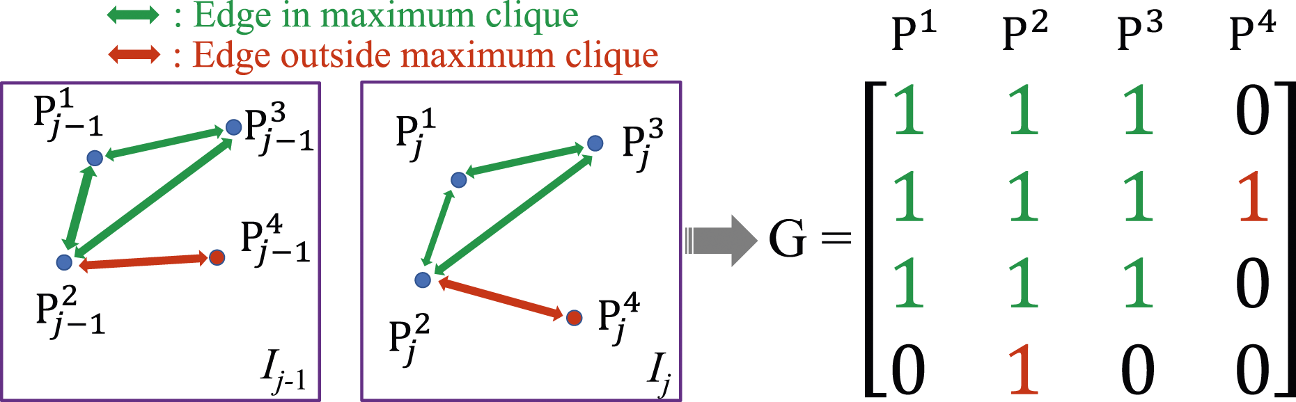P⁴.

4.3. Motion distortion modelling

After the tracked points are associated, they can be used to estimate the motion. However, since the radar scanning rate is slow, they tend to suffer from serious motion distortion as discussed in Sec. 3.3. This can dramatically degrade the accuracy of motion estimation, which is different from most of the vision and LiDAR based methods. Therefore, we explicitly model and compensate for motion distortion in radar pose tracking using an optimization approach.

Assume a full polar radar scan S _j takes Δt seconds to finish. Denote T _w , _j as the pose of radar scan S _j in the world coordinate frame ${\mathrm{ℱ}}_w$ and ${\mathbf{T}}_{j,j_t}$ as the pose of the radar scan in the local frame while capturing its azimuth beam at time t ∈ [ − Δt/2, Δt/2]. Without losing generality, we compensate the motion distortion relative to the central azimuth beam at t = 0, that is, ${\mathrm{ℱ}}_{j_0}$ defines the local coordinate frame ${\mathrm{ℱ}}_j$ of S _j . The motion distortion model is designed to correct detections on each beam of a radar scan, that is, optimally estimating the detections on an undistorted radar image as shown in Figure 6.

Figure 6.

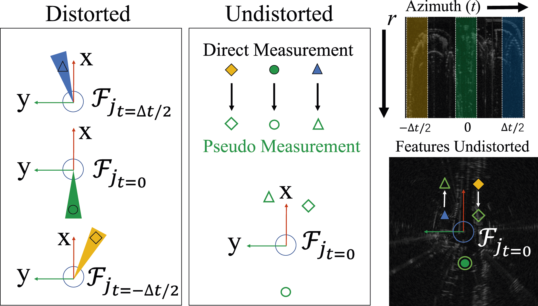
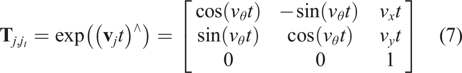
Motion modelling to remove distortion. (Left): For each azimuth angle in a single scan, a radar detection is observed within frame ${\mathrm{ℱ}}_{j_t}$ while moving. (Middle): All the detections are projected onto frame ${\mathrm{ℱ}}_{j_0}$ using the optimized motion model, compensating for motion distortion. (Right): Corresponding azimuth scans of the detections shown on a polar image and the positional changes of detections without distortion in a Cartesian image. All these compensated detections are within frame ${\mathrm{ℱ}}_{j_0}$ .

The radar pose in the world coordinate frame while capturing an azimuth scan at time t can be obtained by

${\mathbf{T}}_{w,j_t}={\mathbf{T}}_{w,j}{\mathbf{T}}_{j,j_t}$

(6)

Consider a constant velocity model in a full scan, we can compute the relative transformation ${\mathbf{T}}_{j,j_t}$ given the velocity v _j , that is

${\mathbf{T}}_{j,j_t}=\exp \left({\left({\mathbf{v}}_{j}t\right)}^{\wedge }\right)=\left[\begin{array}{ccc}\cos \left(v_{\theta }t\right)& -\sin \left(v_{\theta }t\right)& v_{x}t\\ \sin \left(v_{\theta }t\right)& \cos \left(v_{\theta }t\right)& v_{y}t\\ 0& 0& 1\end{array}\right]$

(7)

where  exp () is the matrix exponential map and ∧ is the operation to transform a vector to a matrix. If the ith keypoint ${\mathbf{p}}_w^i$ in the world frame ${\mathrm{ℱ}}_w$ is observed as ${\mathbf{p}}_{j_t}^i$ in the azimuth scan at time t, its motion compensated location is then

${\mathbf{p}}_{j_0}^i={\mathbf{T}}_{j,j_t}{\mathbf{p}}_{j_t}^i$

(8)

In other words, ${\mathbf{p}}_{j_0}^i$ is the compensated location of ${\mathbf{p}}_w^i$ in the local frame ${\mathrm{ℱ}}_{j_0}$ . Therefore, the feature residual between the locally observed and estimated (after motion compensation) locations of this ith keypoint can be computed as:

${\mathbf{e}}_p^i={\rho }_c\left({\mathbf{T}}_{w,j}^{-1}{\mathbf{p}}_w^i-{\mathbf{p}}_{j_0}^i\right)$

(9)

where ρ _c is the Cauchy robust cost function used to account for perspective changes described in 3.3.2.

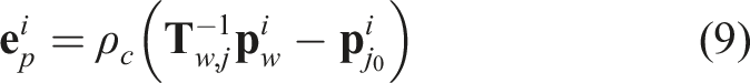
4.4. Optimal motion compensated radar pose tracking

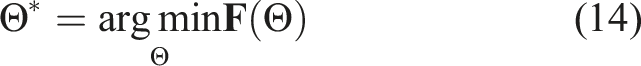
Radar pose tracking aims to find the optimal radar pose T _w , _j and the current velocity v _j while considering the motion distortion. In order to ensure smooth motion dynamics, a velocity error e _v is also introduced as a velocity prior term:

${\mathbf{e}}_v={\mathbf{v}}_j-{\mathbf{v}}_{j,\hspace{0.17em}prior}$

(10)

where v _j , _prior is a prior on the current velocity which is parameterized as

${\mathbf{v}}_{j,prior}=\frac{\log {\left({\left({\mathbf{T}}_{w,j-1}\right)}^{-1}{\mathbf{T}}_{w,j}\right)}^{\vee }}{\mathrm{\Delta }t}$

(11)

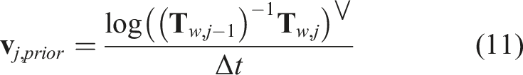
Here, ∨ is the operation to convert a matrix to a vector. This velocity prior term establishes a constraint on velocity changes by considering the previous pose T _w ,_j−1. This prior is crucial to stabilize the optimization. The results with and without this prior are compared in Figure 7. Therefore, the pose tracking optimizes the velocity v _j and the current radar pose T _w , _j by minimizing the cost function including the feature residuals of all the N keypoints tracked in S _j and the velocity prior, that is

${\mathbf{v}}_j^{\ast },{\mathbf{T}}_{w,j}^{\ast }=\underset{{\mathbf{v}}_j,{\mathbf{T}}_{w,j}}{\text{arg\hspace{0.17em}min}}\left\{{\mathbf{e}}_v^T{\mathbf{\Lambda }}_v{\mathbf{e}}_v+{\displaystyle \sum _{i=1}^N{\mathbf{e}}_p^{i^T}}{\mathbf{\Lambda }}_p^i{\mathbf{e}}_p^i\right\}$

(12)

where ${\mathbf{\Lambda }}_p^i$ and Λ _v are the information matrices of the keypoint i and the velocity.

Figure 7.

Odometry trajectories without and with the residual term e _v in the optimization. Without the residual term e _v to correlate pose with velocity, we might obtain an arbitrary solution for pose and velocity. To stabilize the optimization, e _v is needed.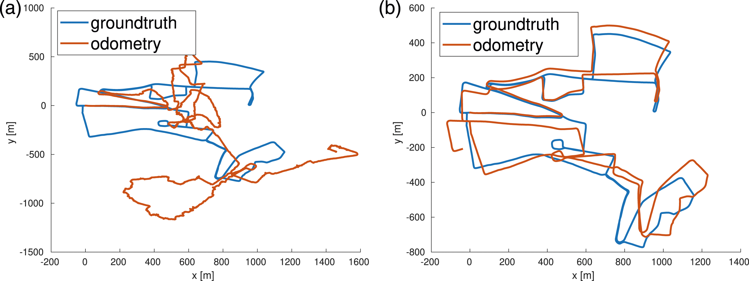

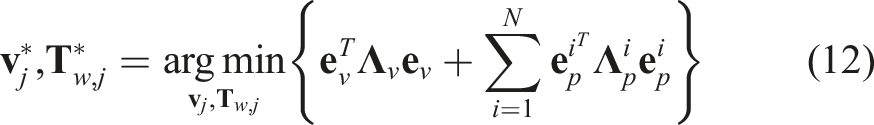
By formulating a state variable Θ containing all the variables to be optimized, that is, the velocity v _j and the current radar pose T _w , _j , and denoting e(Θ) as the residual function containing both ${\mathbf{e}}_p^i$ and e _v , Θ can be solved in an optimization whose factor graph representation is shown in Figure 8. The optimization problem is then framed as finding the minimum of the weighted Sum of Squared Errors cost function:

$\mathbf{F}\left(\mathrm{\Theta }\right)={\displaystyle \sum _i{\mathbf{e}}_i^T}\left(\mathrm{\Theta }\right){\mathbf{W}}_i{\mathbf{e}}_i\left(\mathrm{\Theta }\right)$

(13)

${\mathrm{\Theta }}^{\ast }=\underset{\mathrm{\Theta }}{\text{arg\hspace{0.17em}min}}\mathbf{F}\left(\mathrm{\Theta }\right)$

(14)

where W _i is a symmetric positive definite weighting matrix.

Figure 8.

Factor graph for the motion compensation model.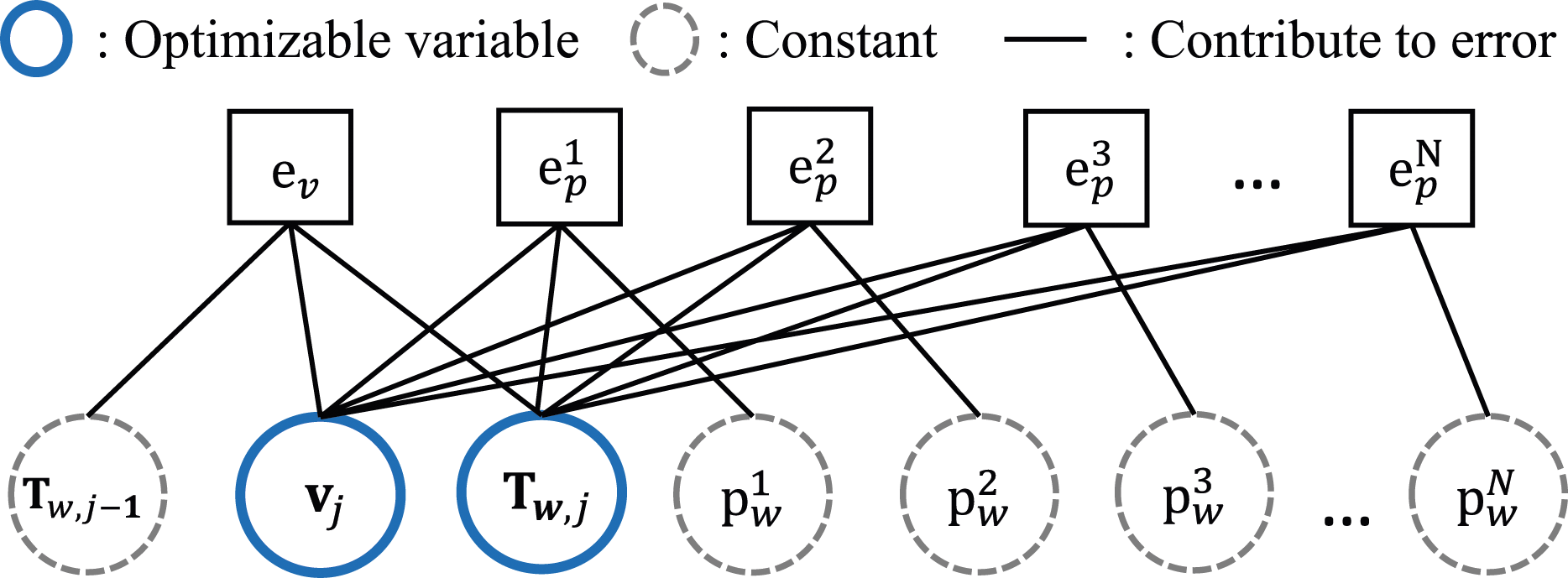

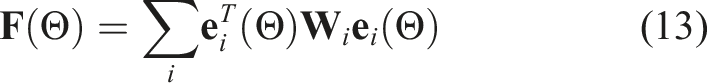
The total cost in 13 is minimized using the Levenberg-Marquardt algorithm. With the initial guess Θ, the residual e _i (ΔΘ⊞Θ) is approximated by its first order Taylor expansion around the current guess Θ:

${\mathbf{e}}_i\left(\mathrm{\Delta }\mathrm{\Theta }\mathrm{⊞}\mathrm{\Theta }\right)\simeq {\mathbf{e}}_i+{\mathbf{J}}_i\mathrm{\Delta }\mathrm{\Theta }$

(15)

where J _i is the Jacobian of e _i evaluated with the current parameters Θ. ⊞ represents a standard addition operator for the velocity variable v _j and a ⊕ operation for the pose variable T _w , _j , that is,  exp ((ΔΘ)^∧) ⋅T _w , _j (Kümmerle et al. (2011), Schubert et al. (2018)). J _i can be decomposed into two parts with respect to the velocity and the pose

${\mathbf{J}}_i=\left[{\mathbf{J}}_{\mathbf{v}},{\mathbf{J}}_{\mathbf{p}}\right]$

(16)

that is, the Jacobian part with respect to the velocity as

${\mathbf{J}}_{\mathbf{v}}=\frac{\partial {\mathbf{e}}_i\left(\mathrm{\Theta }\right)}{\partial \left({\mathbf{v}}_{j}t\right)}\frac{\partial \left({\mathbf{v}}_{j}t\right)}{\partial {\mathbf{v}}_j}$

(17)

and the Jacobian with respect to the pose as

${\mathbf{J}}_{\mathbf{p}}=\frac{\partial {\mathbf{e}}_i\left(\mathrm{\Theta }\right)}{\partial \left({\mathbf{T}}_{w,j}\right)}$

(18)

which is equivalent to computing the Jacobian with respect to zero perturbation ΔΘ _p around the pose (Solà et al. (2018)), that is

$\frac{\partial {\mathbf{e}}_i\left(\mathrm{\Theta }\right)}{\partial \left({\mathbf{T}}_{w,j}\right)}=\frac{\partial {\mathbf{e}}_i\left(\mathrm{\Delta }\mathrm{\Theta }\mathrm{⊞}\mathrm{\Theta }\right)}{\partial \mathrm{\Delta }{\mathrm{\Theta }}_{\mathbf{p}}}$

(19)

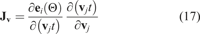
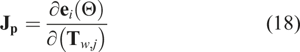
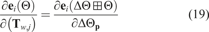
The Levenberg-Marquardt algorithm computes a solution ΔΘ at each iteration such that it minimizes the residual function e _i (ΔΘ ⊞Θ). We refer the reader to (Kümmerle et al. (2011)) for further details on the optimization process.

4.5. New point generation

After tracking the current radar scan S _j , the total number of successfully tracked keypoints is checked to decide whether new keypoints should be generated. If it is below a certain threshold, new keypoints are extracted and added for tracking if they are located in image grids whose total numbers of keypoints are low. Specifically, we divide the radar image into grids and count the number of tracked points in each grid. These grids are then sorted according to the number of keypoints in each of them. For the grids that have fewer number of keypoints, new keypoints are extracted in them before being inserted for tracking. The number of the new keypoints is limited by the maximum number of keypoints in each grid. Once a new keypoint ${\mathbf{p}}_{j_t}^i$ is associated with the current frame S _j , its global position p _w can be derived from

${\mathbf{p}}_w={\mathbf{T}}_{w,j}^{\ast }\exp \left({\left({\mathbf{v}}_j^{\ast }t\right)}^{\wedge }\right){\mathbf{p}}_{j_t}^i$

(20)

using its direct observation of ${\mathbf{p}}_{j_t}^i$ (with distortion). ${\mathbf{T}}_{w,j}^{\ast }$ and ${\mathbf{v}}_j^{\ast }$ are the optimal radar pose and velocity derived in equation (12).

4.6. New keyframe generation

To scale the system in a large-scale environment, we use a pose-graph representation for the map with each node parameterized by a keyframe. Each keyframe which contains a velocity and a pose is connected with its neighbouring keyframes using its odometry derived from the motion estimation. The keyframe generation criterion is similar to that introduced in (Mur-Artal and Tardós (2017)) based on travelled distance and angle.

5. Loop closure and pose graph optimization

Robust loop closure detection is critical to reduce drift in a SLAM system. Although the Bag-of-Words model has proved efficient for visual SLAM algorithms, it is not adequate for radar-based loop closure detection due to three main reasons: first, radar images have less distinctive pixel-wise characteristics compared to optical images, which means similar feature descriptors can repeat widely across radar images causing a large number of incorrect feature matches; second, the multi-path reflection problem in radar can introduce further ambiguity for feature description and matching; third, a small rotation of the radar sensor may produce tremendous scene changes, significantly distorting the histogram distribution of the descriptors. There are some attempts to address this challenge in the context of place recognition (Săftescu et al. (2020), Gadd et al. (2021), Kim et al. (2020)). On the other hand, radar imagery encapsulates valuable absolute metric information, which is inherently missing for an optical image. Therefore, we propose a loop closure technique which captures the geometric scene structure and exploits the spatial signature of reflection density from radar point clouds.

Algorithm 1

Radar Polar Scan to Point Cloud Conversion

Input: Radar polar scan $\mathbf{S}\in {ℝ}^{m\times n}$ ;

Output: Point Cloud $\mathbf{C}\in {ℝ}^{z\times 2}$ ;

Parameters: Minimum peak prominence δ _p and minimum peak distance δ _d;

Initialize empty point cloud set C;

for i ← 1 to m do

 Q^k×1 ← findPeaks (S [i, :], δ _p , δ _d );

 (μ, σ) ← meanAndStandardDeviation (Q^k×1);

 for each peak q in Q do

  if q ≥ (μ + σ) then

   p ← transformPeakToPoint (q, i);

   Add the point p to C;

  end

 end

end

5.1. Point cloud generation

Considering the challenges of radar sensing in Sec. 3.3, we want to separate true targets from the noisy measurements on a polar scan. An intuitive and naive way would be to detect peaks by finding the local maxima from each azimuth reading. However, as shown in Figure 9, the detected peaks can be distributed randomly across the whole radar image, even for areas without a real object, due to the speckle noise described in Sec. 3.3.1. Therefore, we propose a simple yet effective point cloud generation algorithm using adaptive thresholding. We denote the return power of a peak as q, we select peaks which satisfy the following inequality constraint

$q\ge \mu +\sigma$

(21)

where μ and σ are the mean and the standard deviation of the powers of the peaks in one azimuth scan. Estimating the power mean and standard deviation along one azimuth instead of the whole polar image can mitigate the effect of receiver saturation since the radar may be saturated at one direction while rotating. By selecting the peaks whose powers are greater than one standard deviation plus their mean power, the true detections tend to be separated from the false-positive ones. The procedure is shown in Algorithm 1. Once a point cloud C is generated from a radar image, M2DP (He et al. (2016)), a rotation invariant global descriptor designed for 3D point clouds, is adapted for the 2D radar point cloud to describe it for loop closure detection. M2DP computes the density signature of the point cloud on a plane and uses the left and right singular vectors of these signatures as the descriptor.

Figure 9.

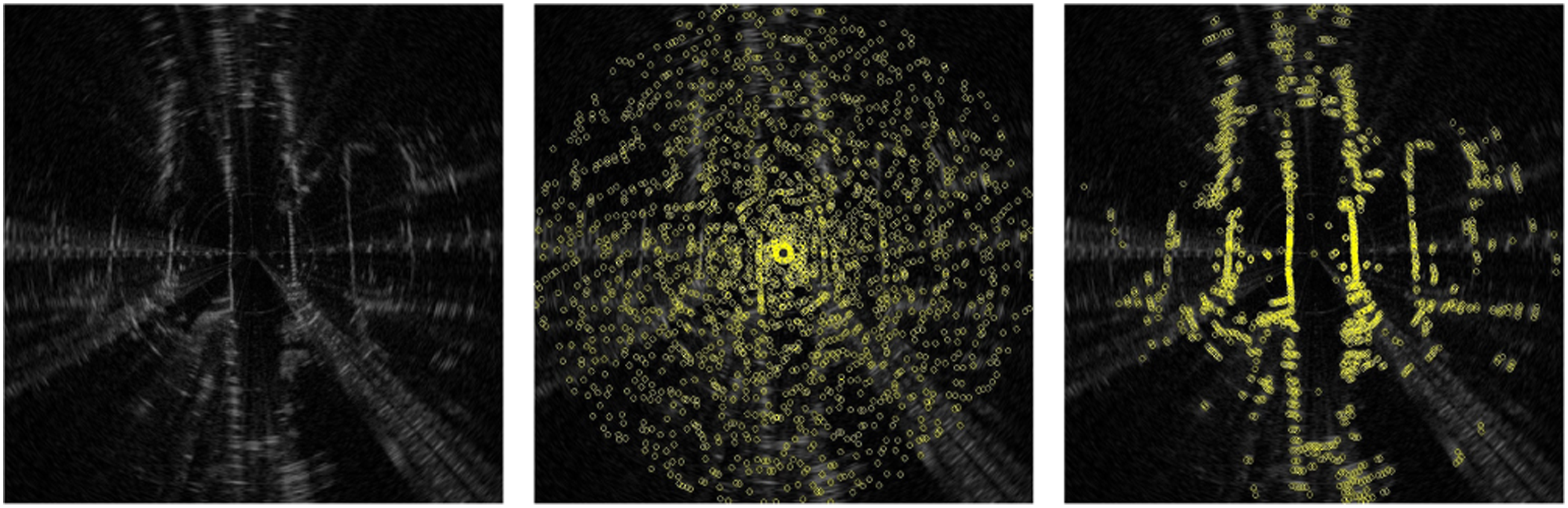
Peak detection in a radar scan. Left: Original Cartesian image. Middle: Peaks (in yellow) detected using a local maxima algorithm. Note that a great amount of peaks detected are due to speckle noise. Right: Peaks detected using the proposed point cloud extraction algorithm which preserves the environmental structure and suppresses detections from multi-path reflection and speckle noise.

5.2. Loop Candidate Rejection with principal component analysis

We leverage principal component analysis (PCA) to determine whether the current frame can be a candidate to be matched with historical keyframes for loop closure detection. After performing PCA on the extracted 2D point cloud C, we compute the ratio r _pca = γ₁/γ₂ between the two eigenvalues γ₁ and γ₂ where γ₁ ≥ γ₂. The frame is selected for loop closure detection if its r _pca is less than a certain threshold δ _pca . The intuition behind this is to detect loop closure mainly on point clouds which have distinctive structural layouts, reducing the possibility of detecting false-positive loop closures. In other words, if γ₁ is dominant (that is, r _pca is big), it is very likely that the radar imagery is collected in an environment, such as a highway or a country road, which exhibits less distinctive structural patterns and layouts and should be avoided for loop closure detection. Some examples are given in Figure 10.

Figure 10.

Radar images with large r _pca tend to be ambiguous.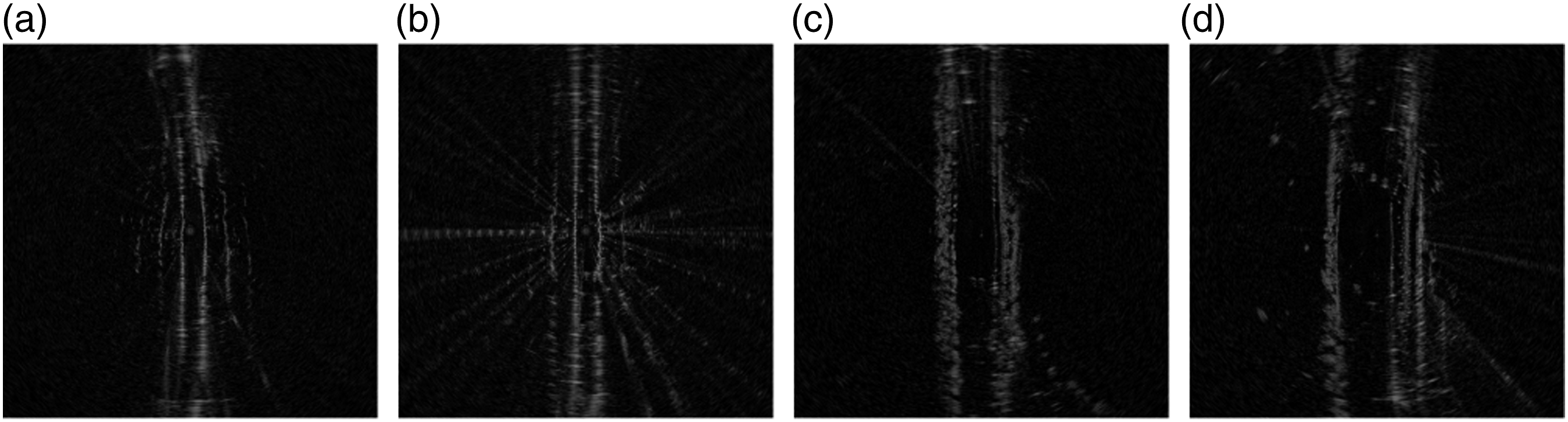

5.3. Relative transformation

Once a loop closure is detected, the relative transformation T _l , _j between the current radar image I _j and the matched radar image I _l is computed. Similar to Sec. 4.1, we also associate keypoints of the two frames by using KLT tracker. The challenge here is that I _l might have a large rotation with respect to I _j , causing the tracker to fail. To address this problem, we estimate firstly the relative rotation between the two frames and align them by using the eigenvectors from the PCA of their point clouds, similar to Sec. 5.2. Then, the keypoints of I _l are tracked through the rotated version of I _j . After obtaining the keypoint association, ICP is used to compute the relative transformation T _l , _j , which is added in the pose graph as a loop closure constraint for pose graph optimization.

5.4. Pose graph optimization

A pose graph is gradually built as the radar moves. Once a new loop closure constraint is added in the pose graph, pose graph optimization is performed. After successfully optimizing the poses of the keyframes, we update the global map points. The g2o (Kümmerle et al. (2011)) library is used in this work for the pose graph optimization.

6. Experimental results

Both quantitative and qualitative experiments are conducted to evaluate the performance of the proposed radar SLAM method using three open radar datasets, covering large-scale environments and some adverse weather conditions.

6.1. Evaluation protocol

We perform both quantitative and qualitative evaluation using different datasets. Specifically, the quantitative evaluation is to understand the pose estimation accuracy of the SLAM system. For Relative/Odometry Error (RE), we follow the popular KITTI odometry evaluation criteria, that is, computing the mean translation and rotation errors from length 100–800 m with a 100 m increment. Absolute Trajectory Error (ATE) is also adopted to evaluate the localization accuracy of full SLAM, in particular after loop closure and global graph optimization. The trajectories of all methods (see full list in Sec. 6.3) are aligned with the ground truth trajectories using a 6 Degree-of-Freedom (DoF) transformation provided by the evaluation tool in (Zhang and Scaramuzza (2018)) for ATE evaluation. On the other hand, the qualitative evaluation focuses on how some challenging scenarios, for example, in adverse weather conditions, influence the performance of various vision, LiDAR and radar-based SLAM systems.

6.2. Datasets

So far there exist three public datasets that provide long-range radar data with dense returns: the Oxford Radar RobotCar Dataset (Barnes et al. (2020a), Maddern et al. (2017)), the MulRan Dataset (Kim et al. (2020)) and the RADIATE Dataset (Sheeny et al. (2021)). We choose the Oxford RobotCar and MulRan datasets for detailed quantitative benchmarking and our RADIATE dataset mainly for qualitative evaluation in our experiments.

6.2.1. Oxford radar RobotCar dataset

The Oxford Radar RobotCar Dataset (Barnes et al. (2020a), Maddern et al. (2017)) provides data from a Navtech CTS350-X Millimetre-Wave W radar for about 280 km of driving in Oxford, UK, traversing the same route 32 times. It also provides stereo images from a Point Grey Bumblebee XB3 camera and LiDAR data from two Velodyne HDL-32E sensors with ground truth pose locations. The radar is configured to provide 4.38 cm and 0.9° resolution in range and azimuth, respectively, with a range up to 163 m. The radar scanning frequency is 4 Hz. See Figure 11 for some examples of data.

Figure 11.

Synchronized radar, stereo, and LiDAR data from the Oxford Radar RobotCar Dataset (Barnes et al. (2020a)).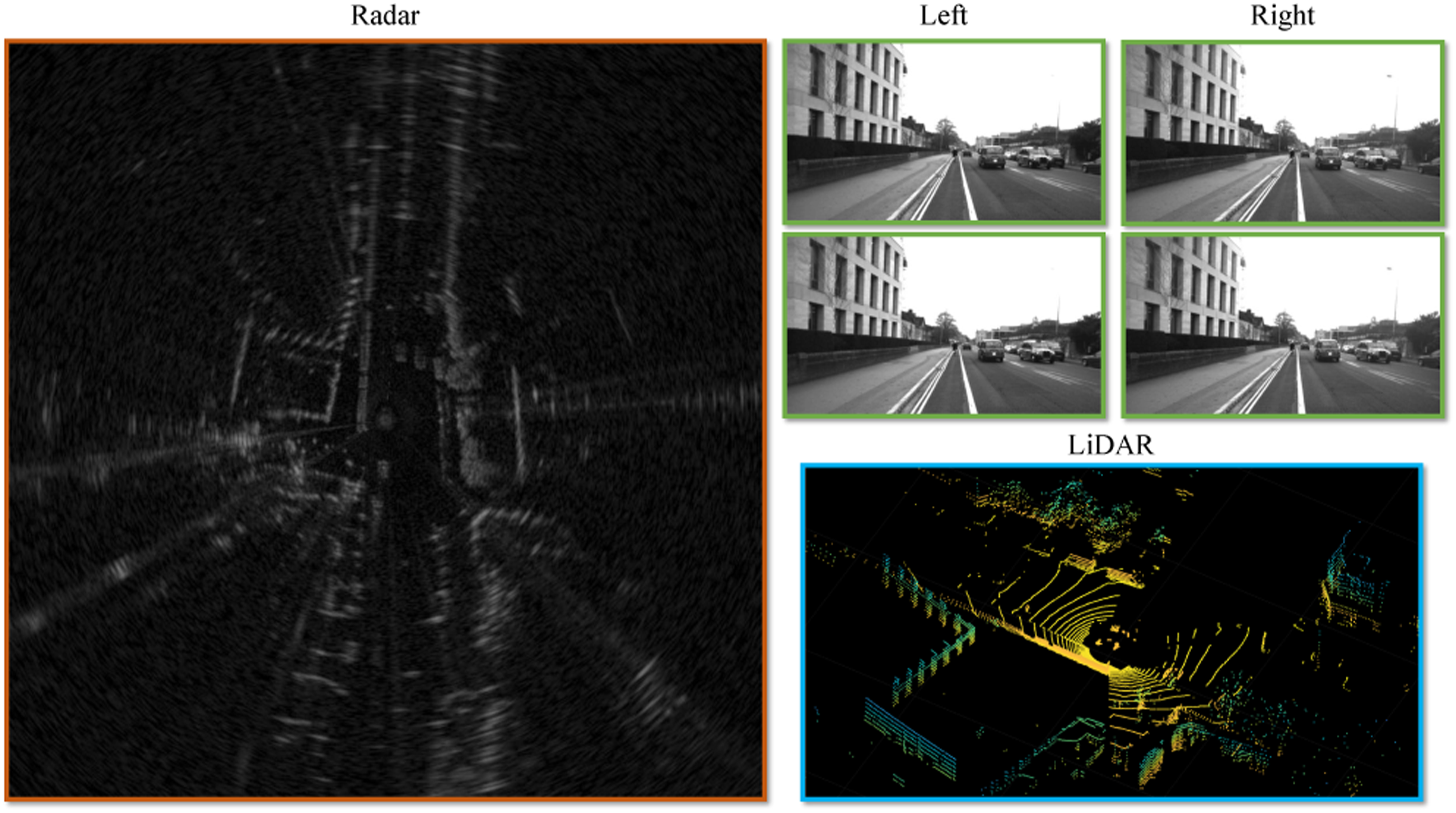

6.2.2. MulRun dataset

The MulRan Dataset (Kim et al. (2020)) provides radar and LiDAR range data, covering multiple cities at different times in a variety of city environments (e.g. bridge, tunnel and overpass). A Navtech CIR204-H Millimetre-Wave FMCW radar is used to obtain radar images with 6 cm range and 0.9° rotation resolutions with a maximum range of 200 m. The radar scanning frequency is also 4 Hz. It also has an Ouster 64-channel LiDAR sensor operating at 10 Hz with a maximum range of 120 m. Different routes are selected for our experiments, including Dajeon Convention Center (DCC), KAIST and Riverside. Specifically, DCC presents diverse structures while KAIST is collected while moving within a campus. Riverside is captured along a river and two bridges with repetitive features. Each route contains three traverses on different days. Some LiDAR and radar data examples are given in Figure 12.

Figure 12.

Radar and LiDAR data from the MulRan Dataset. In Riverside, we can see the repetitive structures of trees and bushes, which makes it challenging for LiDAR based odometry and mapping algorithms (Kim et al. (2020)).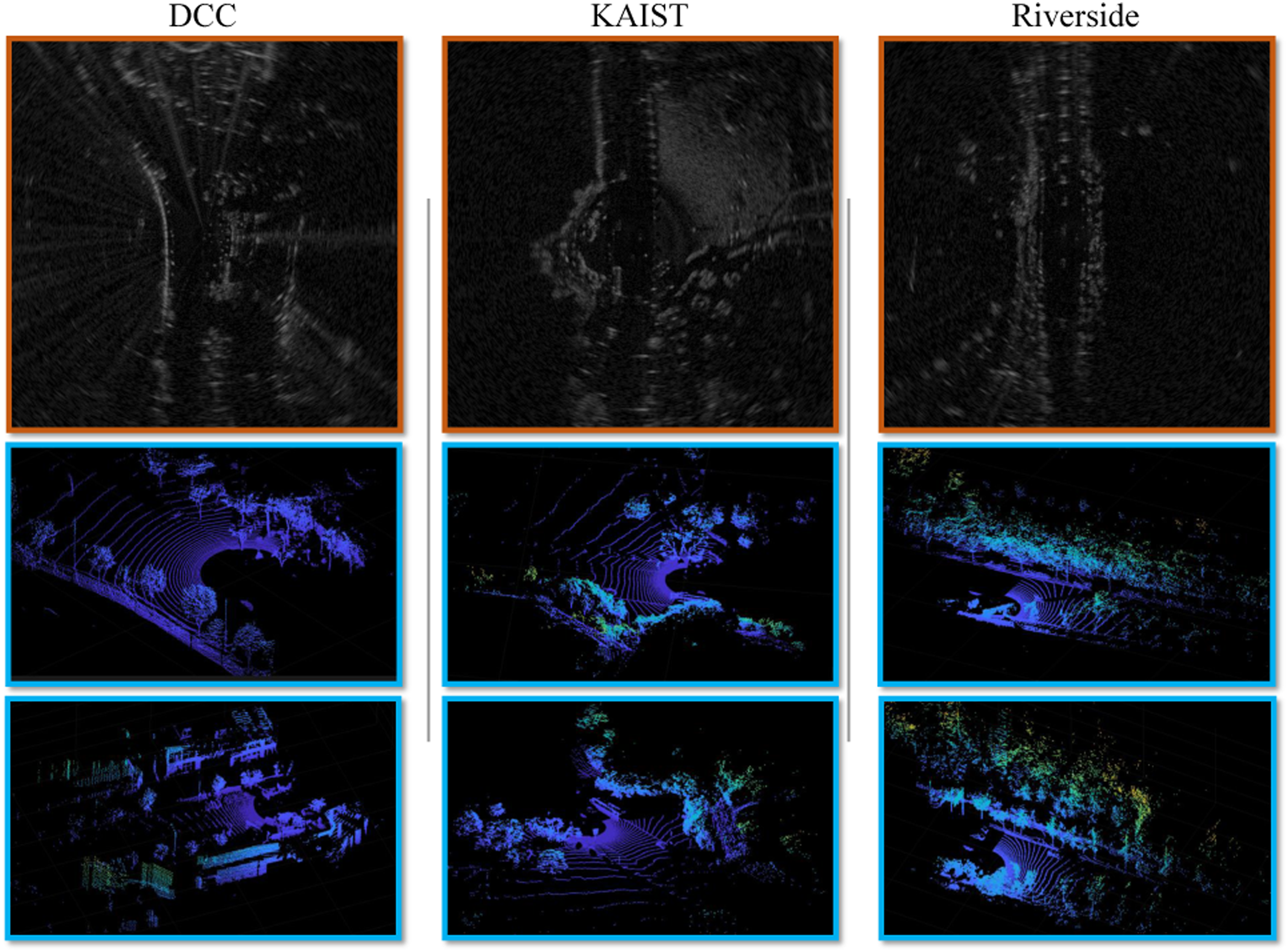

6.2.3. RADIATE dataset

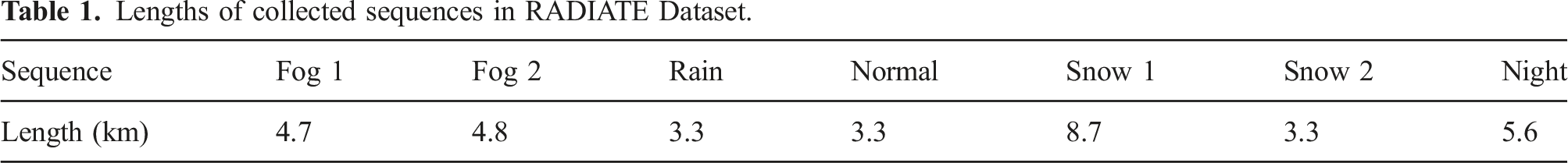
The RADIATE dataset is our recently released dataset which includes radar, LiDAR, stereo camera and GPS/IMU data (Sheeny et al. (2021)). One of its unique features is that it provides data in extreme weather conditions, such as rain and snow, as shown Figure 13. A Navtech CIR104-X radar is used with 0.175 m range resolution and maximum range of 100 m at 4 Hz operating frequency. A 32-channel Velodyne HDL-32E LiDAR and a ZED stereo camera are set at 10 Hz and 15 Hz, respectively. The seven sequences used in this work include 2 fog, 1 rain, 1 normal, 2 snow and 1 night recorded in the City of Edinburgh, UK. Their sequence lengths are given in Table 1. Note that only the rain, normal, snow and night sequences have loop closures and the GPS signal is occasionally lost in the snow sequence.

Figure 13.

Images collected in Snow (left), Fog/Rain (middle), and Night (right). The image quality degrades in these conditions, making it extremely challenging for vision based odometry and SLAM algorithms. Note that for the snow sequence, the camera is completely covered by snow.

Table 1.

Lengths of collected sequences in RADIATE Dataset.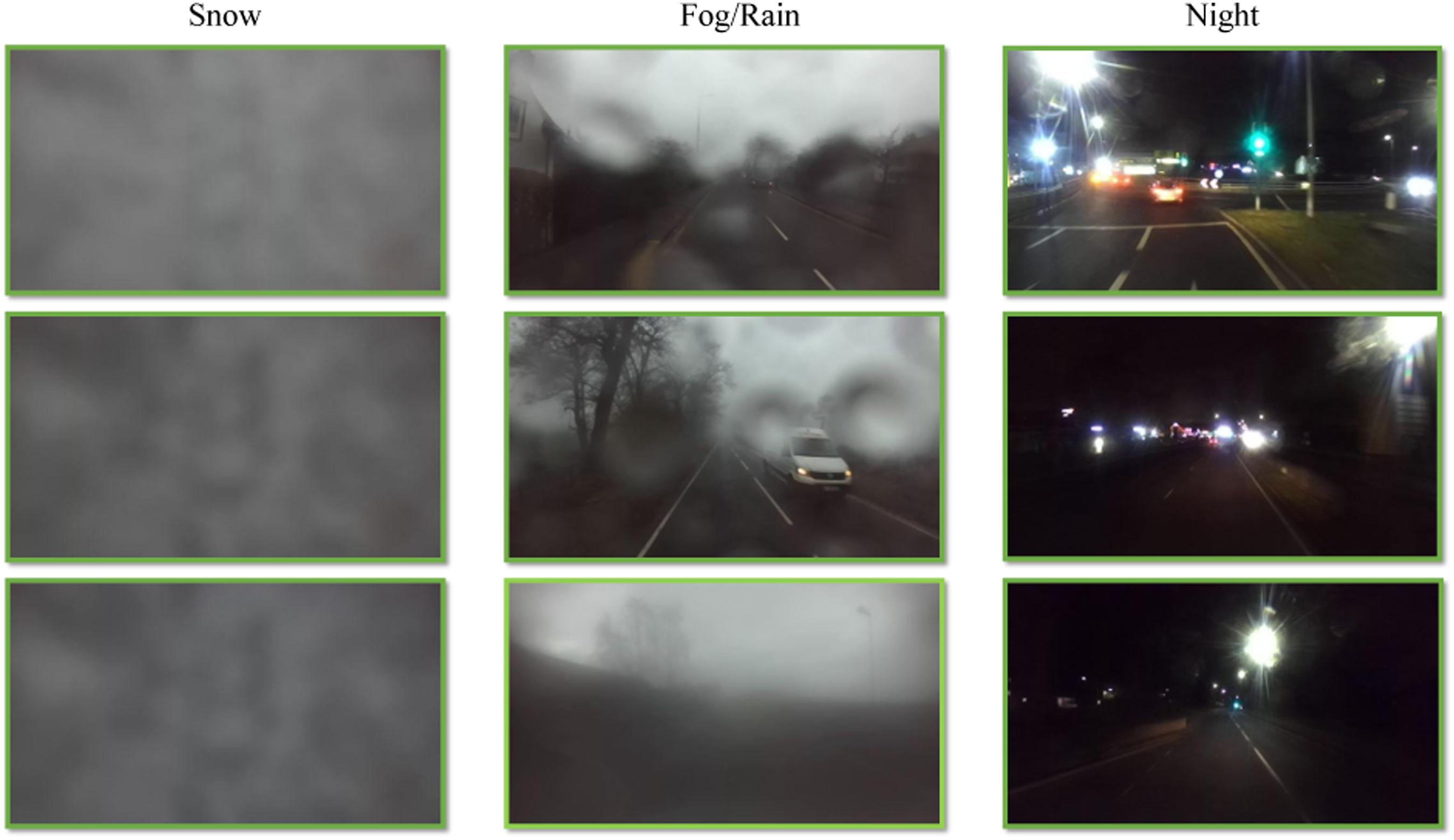

Sequence	Fog 1	Fog 2	Rain	Normal	Snow 1	Snow 2	Night
Length (km)	4.7	4.8	3.3	3.3	8.7	3.3	5.6

6.3. Competing methods and their settings

In order to validate the performance of our proposed radar SLAM system, state-of-the-art odometry and SLAM methods for large-scale environments using different sensor modalities (camera, LiDAR, radar) are chosen. These include ORB-SLAM2 (Mur-Artal and Tardós (2017)), SuMa (Behley and Stachniss (2018)) and our previous version of RadarSLAM (Hong et al. (2020)), as baseline algorithms for vision, LiDAR and radar-based approaches, respectively. For the Oxford Radar RobotCar Dataset, the results reported in (Cen and Newman (2018), Barnes et al. (2020b)) are also included as a radar-based method due to the unavailability of their implementations.

We would like to highlight that we use an identical set of parameters for our radar odometry and SLAM algorithm across all the experiments and datasets. We believe this is worthwhile to tackle the challenge that most existing odometry or SLAM algorithms require some levels of parameter tuning in order to reduce or avoid result degradation.

6.3.1. Stereo vision based ORB-SLAM2

ORB-SLAM2 (Mur-Artal and Tardós (2017)) is a sparse feature based visual SLAM system which relies on ORB features. It also possesses loop closure and pose graph optimization capabilities. Local Bundle Adjustment is used to refine the map point position which boosts the odometry accuracy. Based on its official open-source implementation, we use its stereo setting in all experiments and loop closure is enabled.

6.3.2. LiDAR based SuMa

SuMa (Behley and Stachniss (2018)) is one of the state-of-the-art LiDAR based odometry and mapping algorithms for large-scale outdoor environments, especially for mobile vehicles. It constructs and uses a surfel-based map to perform robust data association for loop closure detection and verification. We employ its open-source implementation and keep the original parameter setting used for KITTI dataset in our experiments.

6.3.3. Radar-based radarSLAM

Our previous version of RadarSLAM (Hong et al. (2020)) extracts SURF features from Cartesian radar images and matches the keypoints based on their descriptors for pose estimation, which is different from the feature tracking technique in this work. It does not consider motion distortion although it includes loop closure detection and pose graph optimization to reduce drift and improve the map consistency. It is named as ‘Baseline Odometry’ and ‘Baseline SLAM’ for comparison.

6.3.4. Cen’s radar odometry

Cen’s method (Cen and Newman (2018)) is one of the first attempts using the Navtech FMCW radar sensor to estimate ego-motion of a mobile vehicle. Landmarks are extracted from polar scans before performing data association by maximizing the overall compatibility with pairwise constraints. Given the associated pairs, SVD is used to find the relative transformation.

6.3.5. Barnes’ radar odometry

Barnes’ method (Barnes et al. (2020b)) leverages deep learning to generate distraction-free feature maps and uses FFT cross correlation to find relative poses on consecutive feature maps. After being trained end-to-end, the system is able to mask out multi-path reflection, speckle noise and dynamic objects. This facilitates the cross correlation stage and produces accurate odometry. The spatial cross-validation results in appendix of (Barnes et al. (2020b)) are chosen for fair comparison.

6.4. Experiments on RobotCar dataset

Results of eight sequences of RobotCar Dataset are reported here for evaluation, that is, 10-11-46-21, 10-12-32-52, 11-14-02-26, 16-11-53-11, 17-13-26-39, 18-14-14-42, 18-14-46-59 and 18-15-20-12. The wide baseline stereo images are used for the stereo ORB-SLAM2 and the left Velodyne HDL-32E sensor is used for SuMa.

6.4.1. Quantitative comparison

The RE and ATE results of each sequence are given in Table 2 and Table 3, respectively. Since the ground truth poses provided by the Oxford Radar RobotCar Dataset are 3-DoF, only the x, y and yaw of the estimated 6-DoF poses of ORB-SLAM2 and SuMa are evaluated. Note that SuMa fails on these eight sequences at 10 − 30% of the full lengths and its results are therefore reported until the point where it fails, and ATE is not applicable due to the lack of fully estimated trajectories. Specifically, the stereo version of ORB-SLAM2 is able to complete seven sequences, successfully close the loops and achieve superior localization accuracy. SuMa also performs accurately when it works although it is less robust on these sequences. This may be due to the large number of dynamic objects, for example, surrounding moving cars and buses. Regarding radar-based approaches, we can see that our proposed radar odometry/SLAM achieves less RE compared to the baseline radar odometry/SLAM and Cen’s method and a similar mean AE to the learning based Barnes’ method. It can also be seen that our proposed radar odometry and SLAM methods achieve better or comparable RE and ATE performance to ORB-SLAM2 and SuMa.

Table 2.

Relative error on Oxford Radar RobotCar Dataset.

	Sequence
Method	10-11-46-21	10-12-32-52	11-14-02-26	16-11-53-11	17-13-26-39	18-14-14-42	18-14-46-59	18-15-20-12	Mean
ORB-SLAM2	6.11/1.7	6.09/1.6	5.63/1.7*26%	6.16/1.7	6.41/1.7	7.05/1.8	7.17/1.9	11.5/3.3	7.01/1.9
SuMa	1.1/0.3*12%	1.1/0.3*20%	3.8/0.5*10%	0.9/0.3*27%	1.1/0.3*23%	0.9/0.1*10%	1.0/0.1*10%	1.0/0.2*20%	1.36/0.3
Cen odometry	N/A	N/A	N/A	N/A	N/A	N/A	N/A	N/A	3.71/0.95
Barnes Odometry	N/A	N/A	N/A	N/A	N/A	N/A	N/A	N/A	2.78/0.85
Baseline Odometry	3.26/0.9	2.98/0.8	4.34/1.2	3.28/0.9	2.92/0.8	3.18/0.9	3.33/1.0	2.85/0.9	3.26/0.9
Baseline SLAM	2.27/0.9	2.16/0.6	2.22/0.7	2.24/0.6	2.45/0.8	2.21/0.7	2.34/0.7	2.24/0.8	2.26/0.7
Our Odometry	2.16/0.6	2.32/0.7	2.02/0.6	2.49/0.7	2.27/0.6	2.29/0.7	2.12/0.6	2.25/0.7	2.24/0.7
Our SLAM	1.96/0.7	1.98/0.6	1.62/0.5	1.81/0.6	1.71/0.5	2.22/0.7	1.68/0.5	1.77/0.6	1.84/0.6

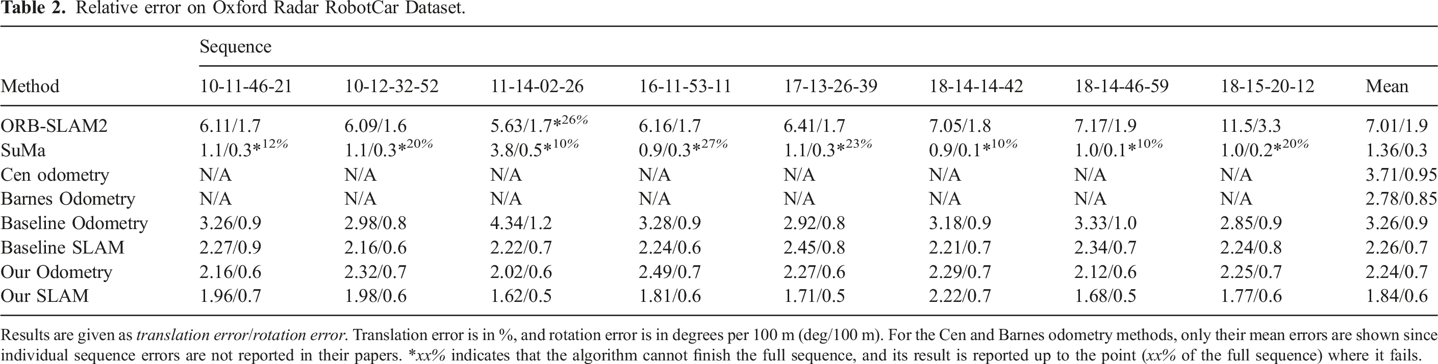
Results are given as translation error/rotation error. Translation error is in %, and rotation error is in degrees per 100 m (deg/100 m). For the Cen and Barnes odometry methods, only their mean errors are shown since individual sequence errors are not reported in their papers. *xx% indicates that the algorithm cannot finish the full sequence, and its result is reported up to the point (xx% of the full sequence) where it fails.

Table 3.

Absolute trajectory error for position (RMSE) on Oxford Radar RobotCar Dataset.

	Sequence
Method	10-11-46-21	10-12-32-52	11-14-02-26	16-11-53-11	17-13-26-39	18-14-14-42	18-14-46-59	18-15-20-12
ORB-SLAM2	7.301	7.961	N/A	3.539	7.609	24.632	9.715	12.174
SuMa	N/A	N/A	N/A	N/A	N/A	N/A	N/A	N/A
Baseline SLAM	58.138	14.598	23.149	12.933	10.898	49.599	23.270	56.422
Our SLAM	13.784	9.593	11.474	7.136	5.835	21.206	6.011	7.740

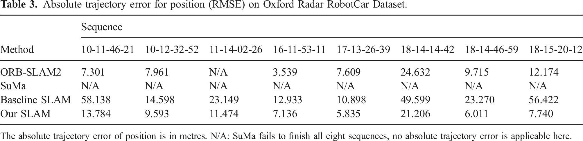
The absolute trajectory error of position is in metres. N/A: SuMa fails to finish all eight sequences, no absolute trajectory error is applicable here.

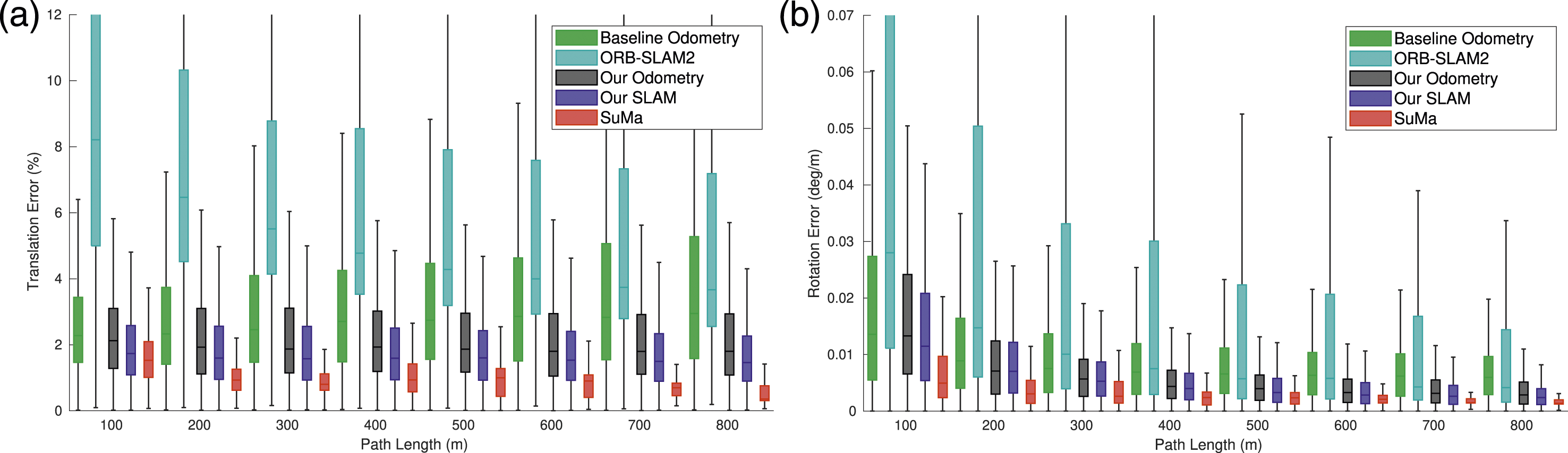
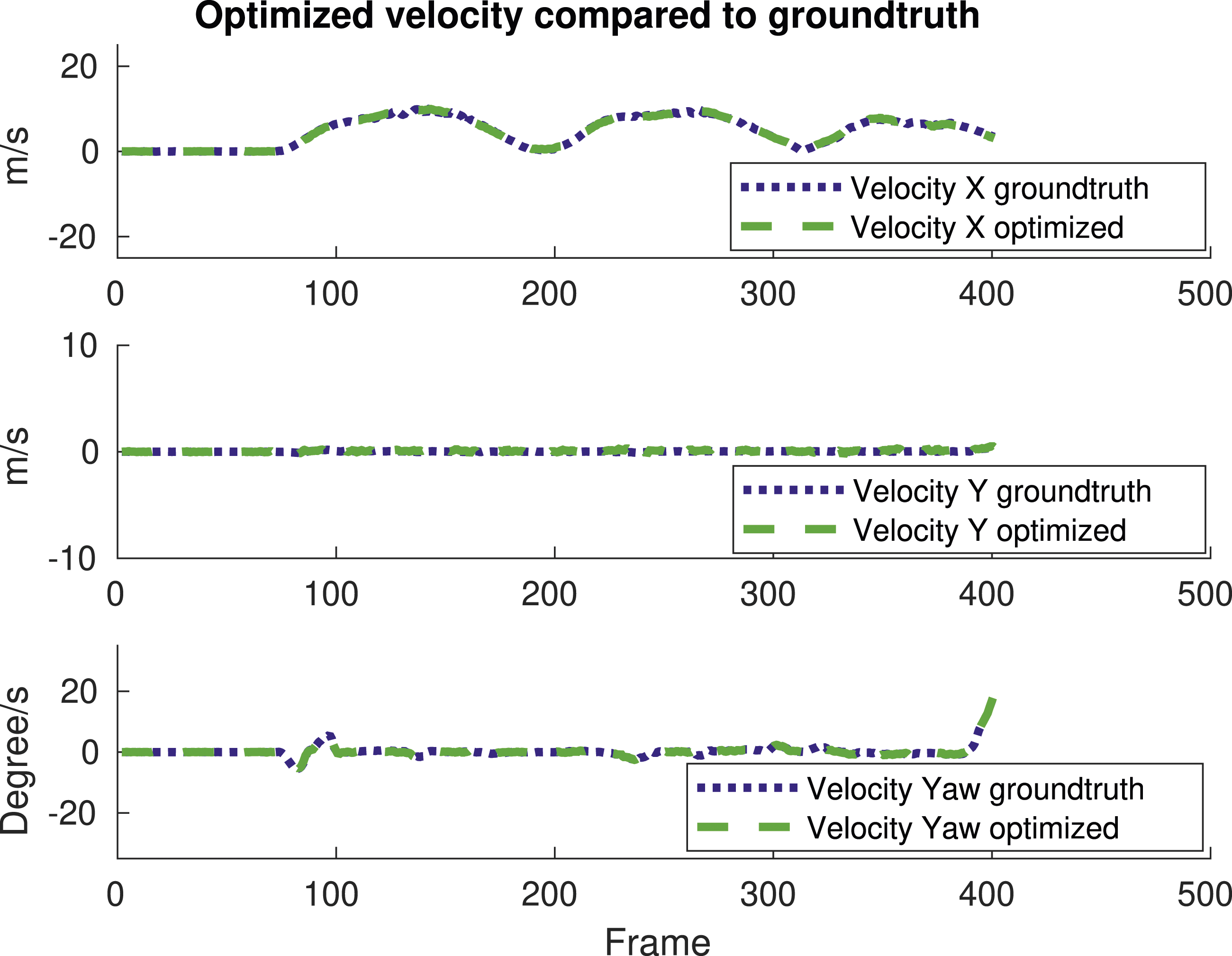
Figure 14 describes the REs of ORB-SLAM2, SuMa, baseline radar odometry and our radar odometry/SLAM algorithms using different path lengths and speeds, following the popular KITTI odometry evaluation protocol. SuMa has the lowest error on both translation and rotation against path lengths and speed until it fails, while our radar SLAM and odometry methods are the second and third lowest, respectively. The low, median and high translation and rotation errors are presented in Figures 15(a) and (b). It can be seen that our SLAM and odometry achieve low values for both translation and rotation errors for different path lengths. The optimized velocities of x, y and yaw are given in Figure 16 compared to the ground truth. The optimized velocities have very high accuracy, which verifies the superior performance of our proposed radar motion estimation algorithm.

Figure 14.

Average error against different path lengths and speeds on Oxford Radar RobotCar Dataset. Note that SuMa’s results are computed up to the point where it fails matching the xx% percentages in Table 2.

Figure 15.

Bar charts for translation and rotation errors against path length on Oxford Radar RobotCar Dataset.

Figure 16.

Optimized x, y and yaw velocities on RobotCar.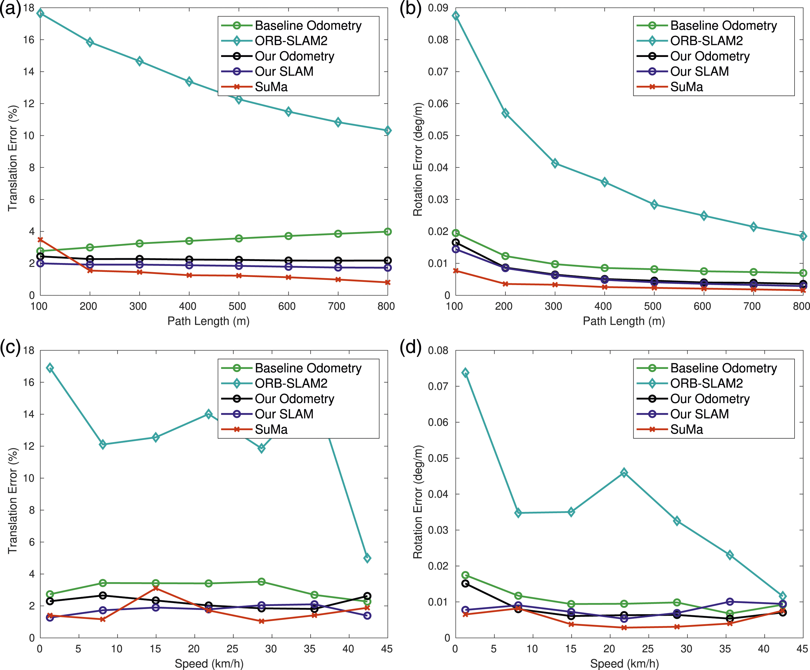

6.4.2. Qualitative comparison

We show the estimated trajectories of six sequences in Figure 17 for qualitative evaluation. For most of the sequences, our SLAM results are closest to the ground truth although the trajectories of baseline SLAM and ORB-SLAM2 are also accurate except for sequence 18-14-14-42. Figure 18 elaborate on the trajectory of each method on sequence 17-13-26-39 for qualitative performance.

Figure 17.

Trajectories for six sequences using different SLAM algorithms on Oxford Radar RobotCar Dataset.

Figure 18.

Trajectories results of different SLAM algorithms on sequence 17-13-26-39 of Oxford Radar RobotCar Dataset.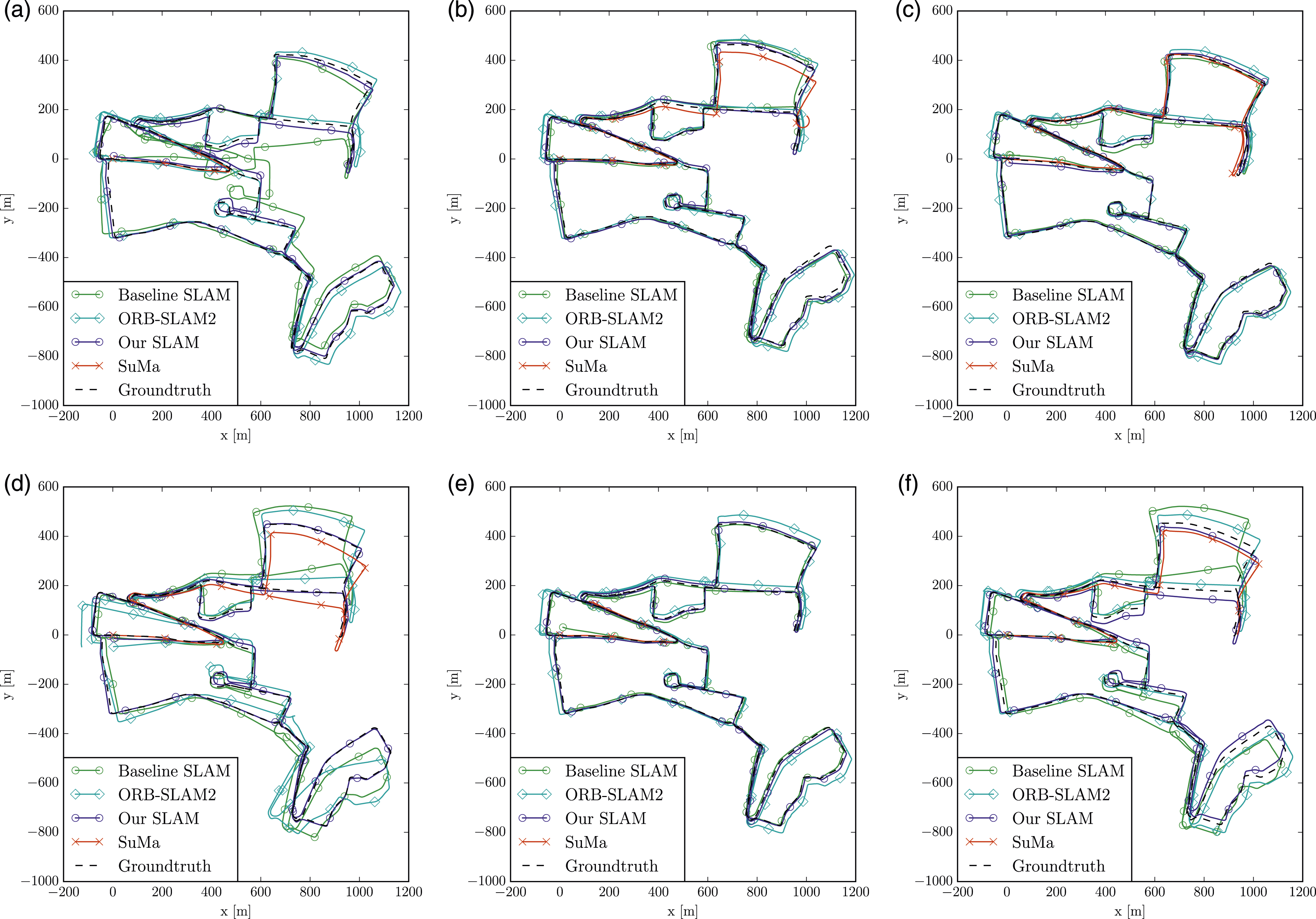

We further compare the proposed radar odometry with the baseline radar odometry (Hong et al. (2020)). Estimated trajectories of three sequences are presented in Figure 19. It is clear that our radar odometry drifts much slower than the baseline radar odometry method, validating the superior performance of the motion estimation algorithm with feature tracking and motion compensation. Therefore, our SLAM system also benefits from this improved accuracy.

Figure 19.

Trajectories of radar odometry results of different algorithms on Oxford Radar RobotCar Dataset.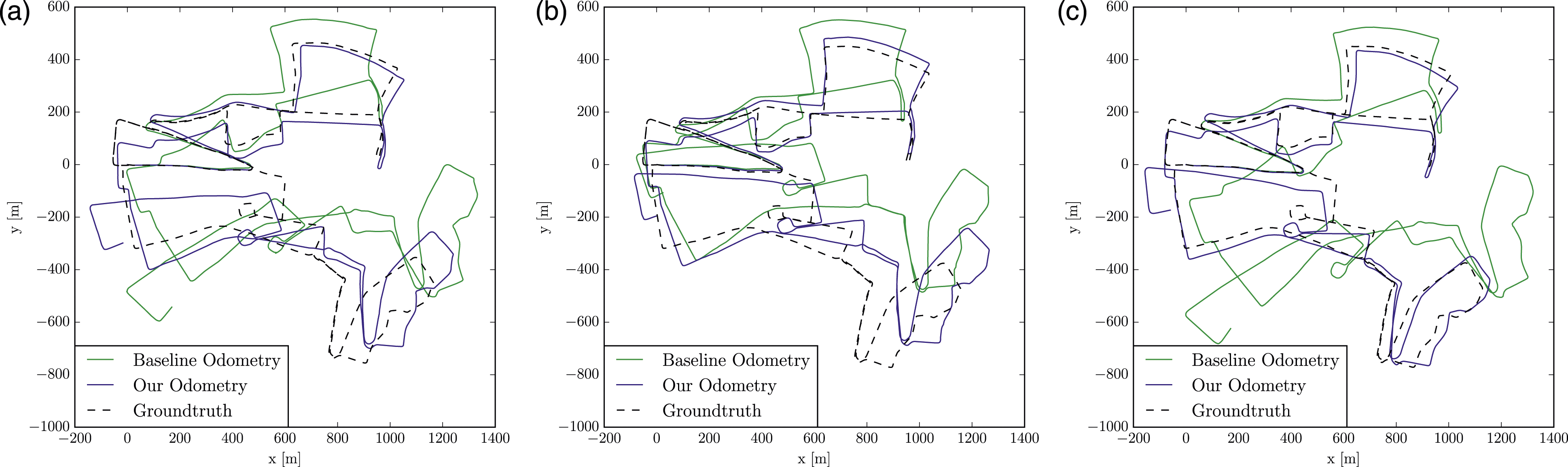

6.5. Experiments on MulRun dataset

The RE and ATE of SuMa, baseline radar odometry/SLAM and our radar SLAM are shown in Table 4 and Table 5. ORB-SLAM2 is not applicable here since MulRan only contains radar and LiDAR data. Similar to the RobotCat dataset, we again transform its provided 6-DoF ground truth poses into 3-DoF for evaluation. Both RE and ATE are evaluated on nine sequences: DCC01, DCC02, DCC03, KAIST01, KAIST02, KAIST03, Riverside01, Riverside02 and Riverside03. In terms of RE, both our odometry and SLAM system achieve comparable or better performance on all sequences.

Table 4.

Relative error on MulRan Dataset.

	Sequence
Method	DCC01	DCC02	DCC03	KAIST01	KAIST02	KAIST03	Riverside01	Riverside02	Riverside03	Mean
SuMa	2.71/0.4	4.07/0.9	2.14/0.6	2.9/0.8	2.64/0.6	2.17/0.6	1.66/0.6*30%	1.49/0.5*23%	1.65/0.4*5%	2.38/0.5
Baseline Odometry	3.35/0.9	2.12/0.6	1.74/0.6	2.32/0.8	2.69/1.0	2.62/0.8	2.70/0.7	3.09/1.1	2.71/0.7	2.59/0.8
Baseline SLAM	3.81/0.9	2.04/0.5	1.90/5.5	2.34/0.7	1.95/0.6	20.1/5.1	3.56/0.9	3.05/6.8	152/0.175	21.1/2.3
Our Odometry	2.70/0.5	1.90/0.4	1.64/0.4	2.13/0.7	2.07/0.6	1.99/0.5	2.04/0.5	1.51/0.5	1.71/0.5	1.97/0.5
Our SLAM	2.39/0.4	1.90/0.4	1.56/0.2	1.75/0.5	1.76/0.4	1.72/0.4	3.40/0.9	1.79/0.3	1.95/0.5	2.02/0.4

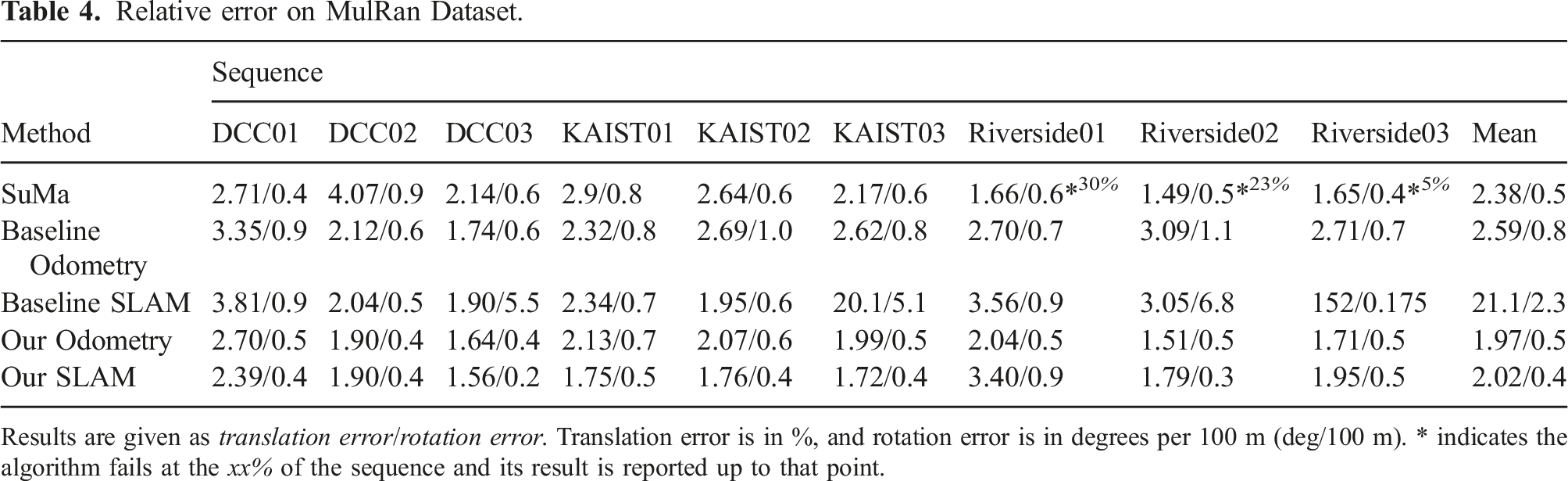
Results are given as translation error/rotation error. Translation error is in %, and rotation error is in degrees per 100 m (deg/100 m). * indicates the algorithm fails at the xx% of the sequence and its result is reported up to that point.

Table 5.

Absolute trajectory error for position (RMSE) on MulRan Dataset.

	Sequence
Method	DCC01	DCC02	DCC03	KAIST01	KAIST02	KAIST03	Riverside01	Riverside02	Riverside03
SuMa	13.509	17.834	29.574	38.693	31.864	45.970	N/A	N/A	N/A
Baseline SLAM	17.458	24.962	76.138	4.931	3.918	50.809	10.531	95.247	1091.605
Our SLAM	12.886	9.878	3.917	6.873	6.028	4.109	9.029	7.049	10.741

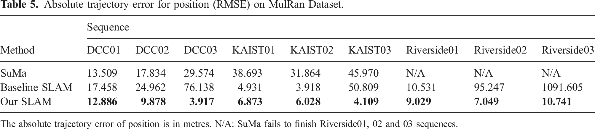
The absolute trajectory error of position is in metres. N/A: SuMa fails to finish Riverside01, 02 and 03 sequences.

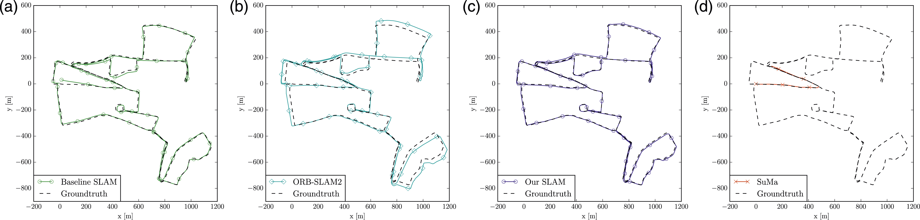
Our odometry method reduces both translation error and rotation errors significantly compared to the baseline. Our SLAM system, to a great extent, outperforms both baseline SLAM and SuMa on ATE. More importantly, only our SLAM reliably works on all nine sequences which cover diverse urban environments. Specifically, the baseline SLAM detects wrong loop closures on sequence KAIST03, Riverside02 and Riverside03 and fails to detect a loop in DCC03, which causes its large ATEs for these sequences. SuMa, on the other hand, fails to finish the sequences Riverside01, 02 and 03, likely due to the challenges of less distinctive structures along the rather open and long road as shown in Figure 20. It can be very challenging to register LiDAR scans accurately in this kind of environment.

Figure 20.

Trajectories results of different SLAM algorithms on sequence Riverside01 of MulRan.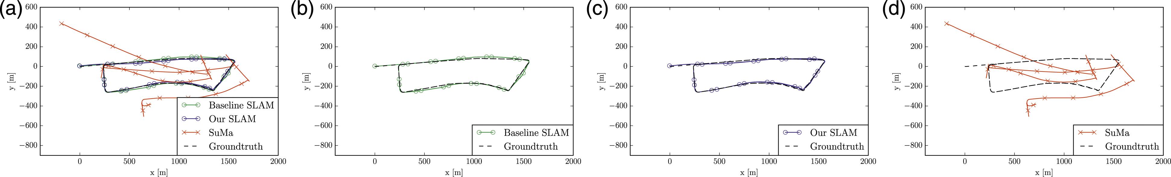

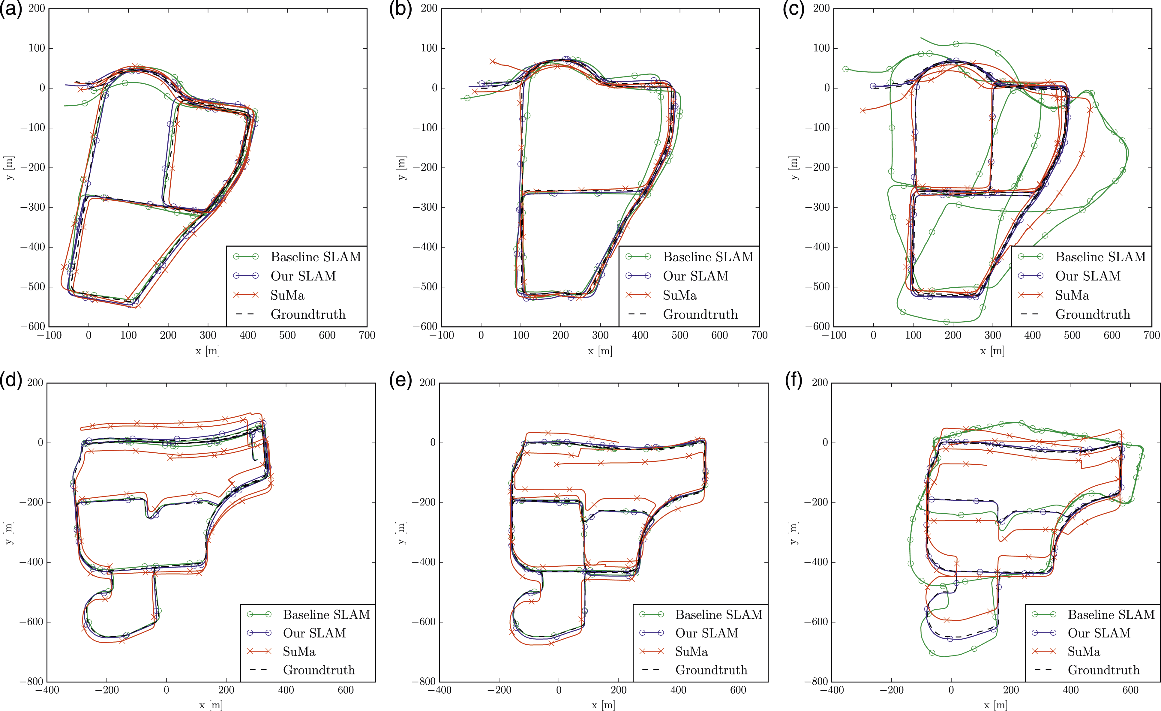
The estimated trajectories on sequences DCC01, DCC02, DCC03, KAIST01, KAIST02, KAIST03 are shown in Figure 21. These qualitative results of the algorithms provide similar observations to the RE and ATE. For clarity, Figure 22 presents trajectories of the SLAM algorithms on Riverside01 in separate figures.

Figure 21.

Riverside scenery of MulRan from Google Street View: repetitive structures are challenging to LiDAR based methods moving on high way.

Figure 22.

Trajectories for six sequences using different SLAM algorithms on MulRan Dataset.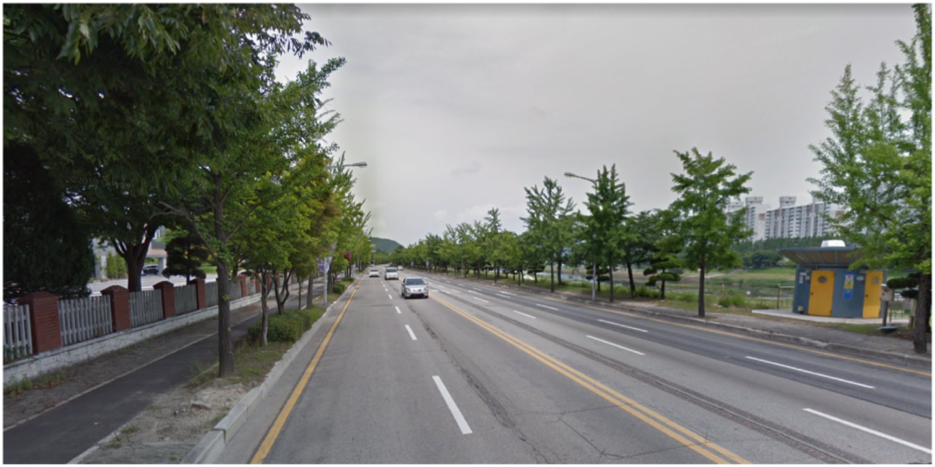

6.6. Experiments on the RADIATE dataset

To further verify the superiority of radar against LiDAR and camera in adverse weathers and degraded visual environments, we perform qualitative evaluation by comparing the estimated trajectories with a high-precision Inertial Navigation System (inertial system fused with GPS) using our RADIATE dataset. Since ORB-SLAM2 fails to produce meaningful results due to the visual degradation caused by water drops, blurry effects in low-light conditions and occlusion from snow (see Figure 13 for example images), its results are not reported in this section.

6.6.1. Experiments in adverse weather

Estimated trajectories of SuMa, baseline and our odometry for Fog 1 and Fog 2 are shown in Figures 23(a) and 23(b), respectively. We can see that our SLAM drifts less than SuMa and the baseline radar SLAM although they all suffer from drift without loop closure. SuMa also loses tracking for sequence Fog 2, which is likely due to the impact of fog on LiDAR sensing.

Figure 23.

Estimated trajectories and ground truth of sequences Fog 1, Fog 2 and Night.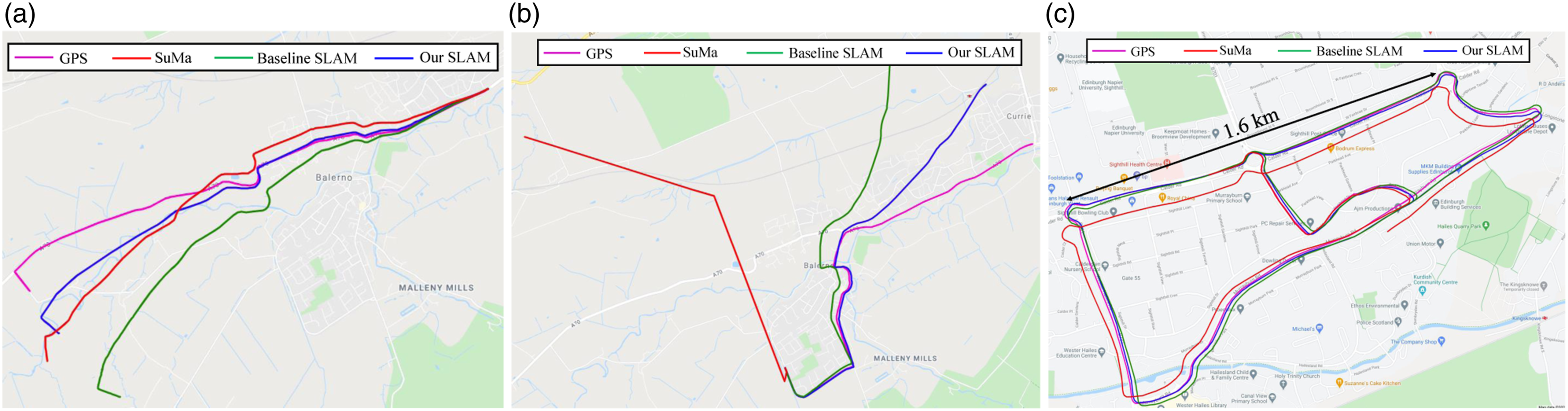

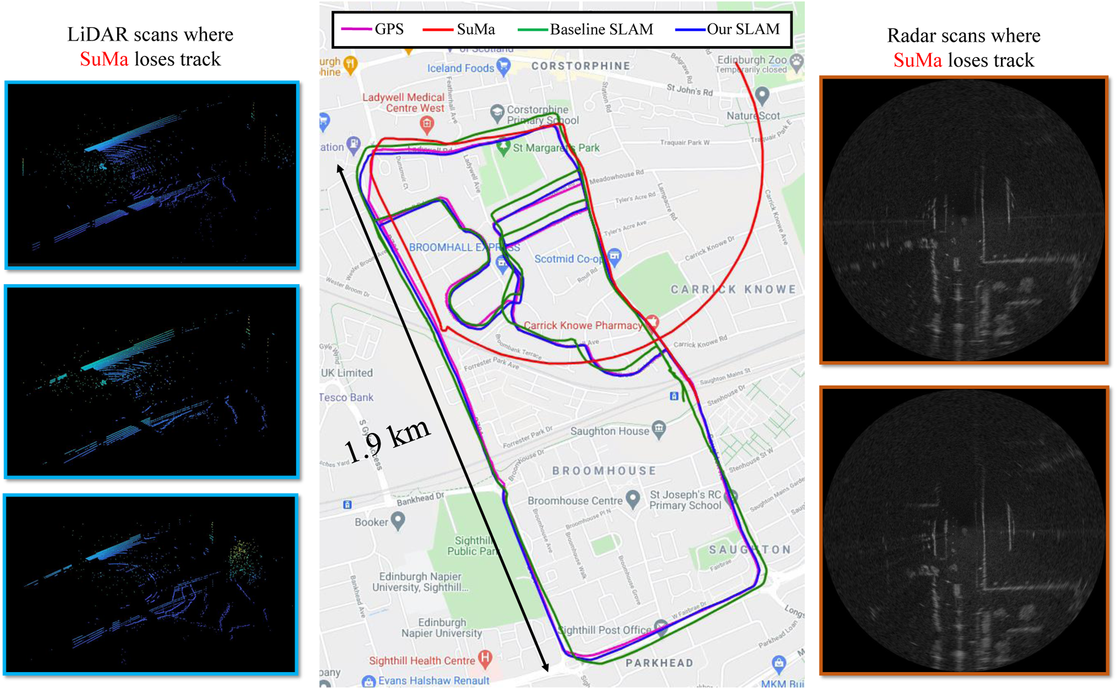
The impact of snowflakes on LiDAR reflection is more obvious. Figure 24 shows the LiDAR point clouds of two of the same places in snowy and normal conditions. Depending on the snow density, we can see two types of degeneration of LiDAR in snow. It is clear that both the number of correct LiDAR reflections and point intensity dramatically drop in snow for place 1, while there are a lot of noisy detections around the origin for place 2. Both cases can be challenging for LiDAR based odometry/SLAM methods. This matches the results of the Snow sequence in Figure 25. Specifically, when the snow was initially light, SuMa was operating well. However, when the snow gradually became heavier, the LiDAR data degraded and eventually SuMa lost track. The three examples of LiDAR scans at the point when SuMa fails are shown in Figure 25. The very limited surrounding structures sensed by LiDAR makes it extremely challenging for LiDAR odometry/SLAM methods like SuMa. In contrast, our radar SLAM method is still able to operate accurately in heavy snow, estimating a more accurate trajectory than the baseline SLAM.

Figure 24.

Two types of LiDAR degeneration. (a, b): Place 1 with less reflection from the scene. (c, d): Place 2 with many noisy detections from snowflakes around.

Figure 25.

Results on the Snow sequence of the RADIATE dataset. Left: LiDAR scans when SuMa loses track. Note the noisy LiDAR reflection of snowflakes. Middle: GPS and estimated trajectories on Google Map. Right: Radar images when SuMa loses track.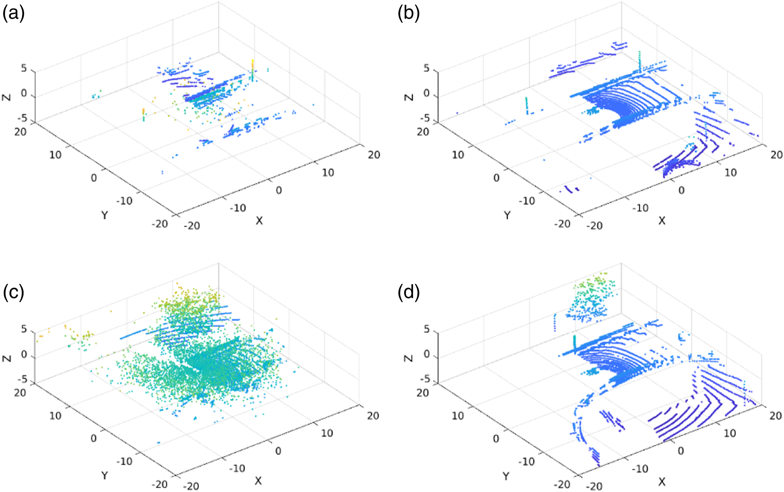

6.6.2. Experiments on the same route in different weathers

To compare different algorithms’ performance on the same route but in different weather conditions, we also provide results here in normal weather, rain and snow conditions, respectively. The estimated trajectories of SuMa, baseline SLAM and our SLAM result in normal weather are shown in Figure 26(a) while for the Rain sequence these are shown in Figure 26(b). In the Rain sequence, there is moderate rain. LiDAR based SuMa is slightly affected, and as we can see at the beginning of the sequence, SuMa estimates a shorter length. Our radar SLAM also performs better than the baseline SLAM. In the Snow 2 sequence, there is moderate snow, and the results are shown in Figure 26(c). The Snow 2 sequence was taken while moving quickly. Therefore, without motion compensation, the baseline SLAM drifts heavily and cannot close the loop while our SLAM consistently performs well. Hence, the results in Figure 26 once again confirm that our proposed SLAM system is robust in all weather conditions.

Figure 26.

(a)–(c): Estimated trajectories and ground truth on multi-session traversals in normal, rain and snow conditions. (d) Top: image data in normal weather captured by our stereo camera, centre: image data in rain captured by our stereo camera, bottom: image data in snow captured by our phone for reference.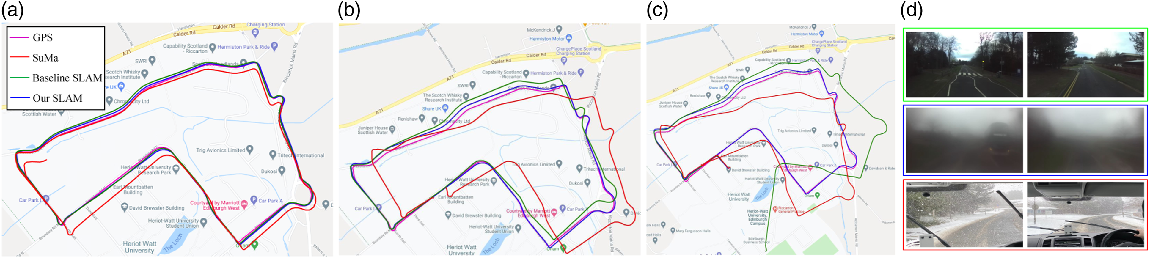

6.6.3. Experiments at night

The estimated trajectories of SuMa, baseline SLAM and our SLAM on the Night sequence are shown in Figure 23(c). LiDAR based SuMa is almost unaffected by the dark night although it does not detect the loops. Both baseline and our SLAM perform well in the night sequence, producing more accurate trajectories after detecting loop closures.

6.7. Average completion percentage

We calculate the average completion percentage for each competing algorithm on each dataset, to evaluate the robustness of each algorithm representing a different sensor modality. The number of frames that a method completed before losing tracking is denoted as K _completed while the total number of frames is denoted as K _total . The metric is computed as:

$Percentage=K_{completed}/K_{total}\ast 100\%$

(22)

The MulRan dataset does not include camera data so it is shown as N/A for ORB-SLAM2. In the RADIATE dataset, the camera is either blocked by snow or blurred in the night so ORB-SLAM2 fails to initialize and it is also shown as N/A. In Table 6 we can see that only the radar-based methods are reliable and completed in all cases. Neither vision based nor LiDAR based methods manage to finish on all three datasets.

Table 6.

Completion Percentage %.

	Dataset
Method	Oxford	MulRan	RADIATE
SuMa	20	72	63
Baseline SLAM	100	100	100
ORB-SLAM2	90	N/A	N/A
Our SLAM	100	100	100

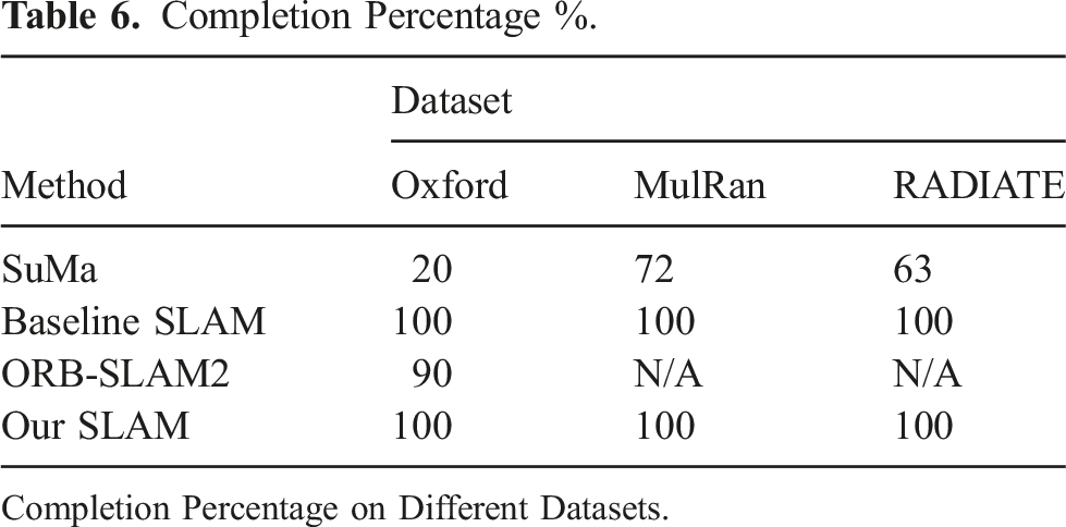
Completion Percentage on Different Datasets.

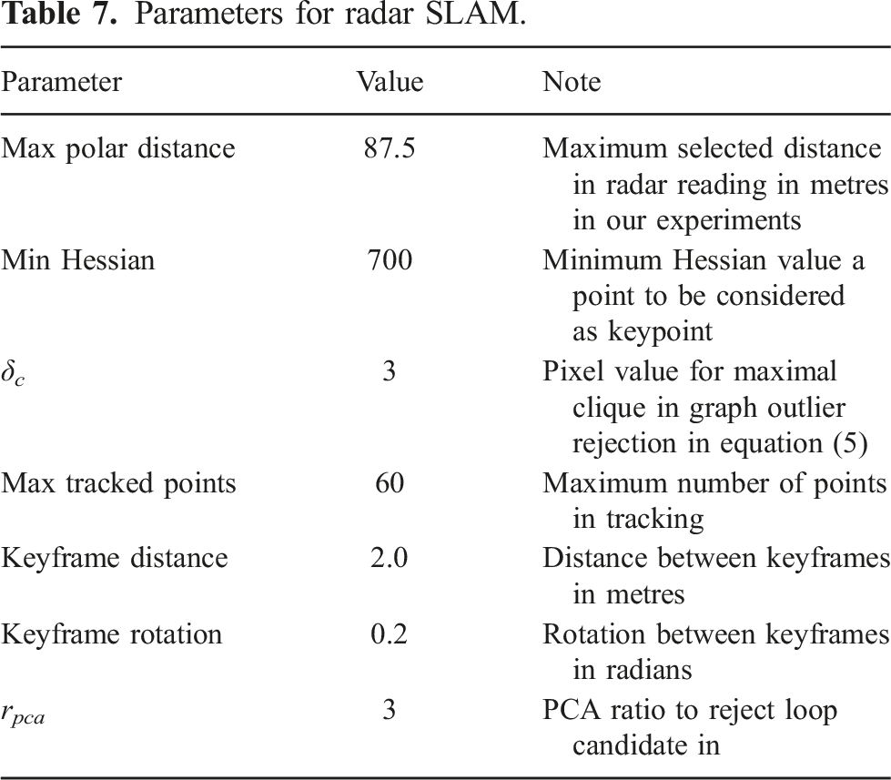
6.8. Parameters used

The same set of parameters provided in Table 7 is employed in all the experiments, covering different cities, radar resolutions and ranges, weather conditions, road scenarios, etc. This selected set of parameters is tuned using the 16-13-09-37 sequence in the Oxford Radar RobotCar Dataset.

Table 7.

Parameters for radar SLAM.

Parameter	Value	Note
Max polar distance	87.5	Maximum selected distance in radar reading in metres in our experiments
Min Hessian	700	Minimum Hessian value a point to be considered as keypoint
δ c	3	Pixel value for maximal clique in graph outlier rejection in equation (5)
Max tracked points	60	Maximum number of points in tracking
Keyframe distance	2.0	Distance between keyframes in metres
Keyframe rotation	0.2	Rotation between keyframes in radians
r pca	3	PCA ratio to reject loop candidate in

6.9. Runtime

The system is implemented in C++ without a GPU. The computation time of a tracking thread is shown in Figure 27 showing that our proposed system runs at 8 Hz, which is twice as fast as the 4 Hz radar frame rate, on a laptop with an Intel i7 2.60 GHz CPU and 16 GB RAM. The loop closure and pose graph optimization are performed with an independent thread which does not affect our real-time performance.

Figure 27.

Computation time of tracking on the Rain sequence.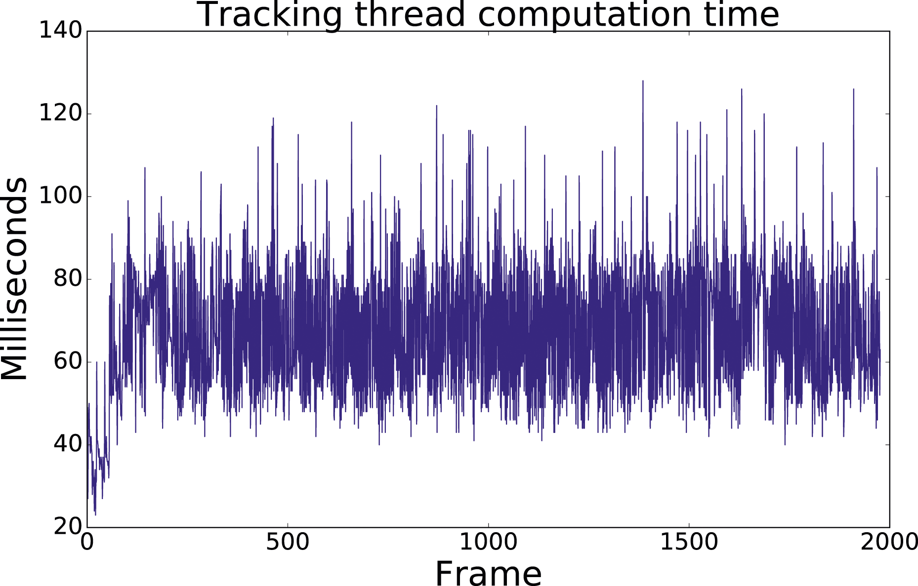

7. Conclusion

In this paper, we have presented a FMCW radar-based SLAM system that includes pose tracking, loop closure and pose graph optimization. To address the motion distortion problem in radar sensing, we formulate pose tracking as an optimization problem that explicitly compensates for the motion without the aid of other sensors. A robust loop closure detection scheme is specifically designed for the FMCW radar. The proposed system is agnostic to the radar resolutions, radar range, environment and weather conditions. The same set of system parameters is used for the evaluation of three different datasets covering different cities and weather conditions.

Extensive experiments show that the proposed FMCW radar SLAM algorithm achieves comparable localization accuracy in normal weather compared to the state-of-the-art LiDAR and vision based SLAM algorithms. More importantly, it is the only one that is resilient to adverse weather conditions, for example, snow and fog, demonstrating the superiority and promising potential of using FMCW radar as the primary sensor for long-term mobile robot localization and navigation tasks. However, our current radar SLAM system depends on an expensive and cumbersome radar sensor. We aim to extend its application on some low-cost, lightweight radar sensors in future. For future work, we also seek to use the map built by our SLAM system and perform long-term localization on it across all weather conditions.

Supplemental Material