
Abstract
In this article, we propose deep visual reasoning, which is a convolutional recurrent neural network that predicts discrete action sequences from an initial scene image for sequential manipulation problems that arise, for example, in task and motion planning (TAMP). Typical TAMP problems are formalized by combining reasoning on a symbolic, discrete level (e.g., first-order logic) with continuous motion planning such as nonlinear trajectory optimization. The action sequences represent the discrete decisions on a symbolic level, which, in turn, parameterize a nonlinear trajectory optimization problem. Owing to the great combinatorial complexity of possible discrete action sequences, a large number of optimization/motion planning problems have to be solved to find a solution, which limits the scalability of these approaches. To circumvent this combinatorial complexity, we introduce deep visual reasoning: based on a segmented initial image of the scene, a neural network directly predicts promising discrete action sequences such that ideally only one motion planning problem has to be solved to find a solution to the overall TAMP problem. Our method generalizes to scenes with many and varying numbers of objects, although being trained on only two objects at a time. This is possible by encoding the objects of the scene and the goal in (segmented) images as input to the neural network, instead of a fixed feature vector. We show that the framework can not only handle kinematic problems such as pick-and-place (as typical in TAMP), but also tool-use scenarios for planar pushing under quasi-static dynamic models. Here, the image-based representation enables generalization to other shapes than during training. Results show runtime improvements of several orders of magnitudes by, in many cases, removing the need to search over the discrete action sequences.
Keywords
1. Introduction
A major challenge in sequential manipulation problems is that they inherently involve discrete and continuous aspects. To account for this hybrid nature of manipulation, task and motion planning (TAMP) problems are usually formalized by combining reasoning on a symbolic, discrete level with continuous motion planning. The symbolic level, e.g., defined in terms of first-order logic, proposes high-level discrete action sequences for which the motion planner, e.g., nonlinear trajectory optimization or a sampling-based method, tries to find configurations and motions that fulfill the requirements induced by the high-level action sequence or return that the action sequence is infeasible. Although most TAMP approaches focus on kinematic tasks such as pick and place, the hybrid nature of manipulation more broadly appears in manipulation planning through contacts, where it is typically addressed in terms of mixed integer optimization formulations.
Owing to the high combinatorial complexity of possible discrete action sequences or integer assignments, a large number of (potentially hard) motion planning problems have to be solved to find a solution to the overall TAMP/manipulation problem. This is mainly caused by the fact that many TAMP problems are difficult, because, mostly due to kinematic limits and geometric constraints, the majority of action sequences are actually infeasible. Moreover, it typically takes more computation time for a motion planner to reliably detect infeasibility of a high-level action sequence than to find a feasible motion when it exists. Proving infeasibility is, in many cases, not even possible. In addition, for a feasible action sequence, the resulting motion planning problem in itself is often non-trivial and hard to solve. Consequently, sequential manipulation problems, which intuitively seem simple, can take a very long time to solve.
To overcome this combinatorial complexity, we aim to learn to predict promising action sequences from the scene as input. Using this prediction as a search heuristic on the symbolic level, we can drastically reduce the number of motion planning problems that need to be evaluated. Ideally, we seek to directly predict a feasible and cost-efficient action sequence, requiring only a single motion planning problem to be solved.
However, learning to predict such action sequences imposes multiple challenges. First, the objects in the scene and the goal have to be encoded as input to the predictor in a way that enables similar generalization capabilities to classical TAMP approaches with respect to scenes with many and changing numbers of objects and goals. Second, the large variety of such scenes and goals, especially if multiple objects are involved, makes it difficult to generate a sufficient dataset.
Recently, Wells et al. (2019) and Driess et al. (2020b) proposed a classifier that predicts the feasibility of a motion planning problem resulting from a discrete decision in the task domain. However, a major limitation of their approaches is that the feasibility for only a single action is predicted, whereas the combinatorial complexity of TAMP especially arises from action sequences and it is not straightforward to utilize such a classifier for action sequence prediction within TAMP.
To address these issues, we train a neural network to predict action sequences from the initial scene and the goal as input. An important question is how the objects in the scene and the goal can be encoded as input to the predictor to ensure strong generalization. By encoding the objects (and the goal) in the image space, we show that the network is able to generalize to scenes with many and changing numbers of objects with only little runtime increase, although it has been trained on only a fixed number of objects.
Compared with a purely discriminative model, because the predictions of our network are goal-conditioned, we do not rely on the network to search over many sequences, but can directly generate promising sequences with the network efficiently.
The predicted action sequences parameterize a nonlinear trajectory optimization problem that optimizes a globally consistent path fulfilling the requirements induced by the actions. This not only allows us to solve typical kinematic problems such as pick and place, but also problems that involve dynamic models. In our case, we build upon the contact formulation from Toussaint et al. (2020) to solve manipulation problems where the robot has to utilize a hook-shaped tool to push and/or pull an object to a desired target location. In order to make this possible, we extend the formulation from Toussaint et al. (2020) by introducing additional discrete decisions that model which part of the tool should establish contact with which side of the object. This robustifies the convergence of the optimizer, but also introduces additional combinatorics, which we can tackle with our proposed network. For this scenario, we demonstrate another advantage of the image-based representation, namely that the network can also generalize to other shapes than during training, because the side to push on the object is also encoded in the image space.
To summarize, our main contributions are as follows.
A convolutional, recurrent neural network (RNN) that predicts from an initial segmented scene image and a task goal promising action sequences, which parameterize a nonlinear trajectory optimization problem, to solve the TAMP problem.
A way to integrate this network into the tree search algorithm of the underlying TAMP framework.
We demonstrate that the network generalizes to situations with many and varying numbers of objects in the scene, although it has been trained on only two objects at a time.
We demonstrate the method not only on typical kinematic pick-and-place scenarios, but also in a scenario where a hook-shaped tool has to be used to push/pull an object to a desired target location.
The image representation enables the network to generalize to other shapes than during training for the pushing scenario.
From a methodological point of view, this work combines nonlinear trajectory optimization, first-order logic reasoning and deep convolutional RNNs.
The present work is an extended version of Driess et al. (2020a). Apart from more in-depth explanations, we include a new set of experiments on a tool-use pushing scenario (Section 5.3), where we also show generalization capabilities to other shapes than during training. Moreover, we provide more evaluations of the existing experiments, e.g., with an investigation of the data efficiency of the approach. Furthermore, we extend the framework to not only being able to find feasible solutions as in the original work, but also taking the trajectory costs into account.
The rest of the article is organized as follows. We describe logic geometric programming (LGP) as the TAMP framework of this work in Section 3. Then, in Section 4, the deep visual reasoning neural network methodology, its architecture, and how it can be integrated into the LGP tree search algorithm is proposed. In Section 4.5, we discuss the relation of our proposed network to offline reinforcement learning (RL). Sections 5.2 and 5.3 present the results of the pick and place and the pushing experiments, respectively. A discussion about the strengths and limitations of the framework can be found in Section 6.
2. Related work
2.1. Learning to plan
There is great deal of interest in learning to mimic planning itself. The architectures in Tamar et al. (2016), Okada et al. (2017), Srinivas et al. (2018), and Amos et al. (2018) resemble value iteration, path integral control, gradient-based trajectory optimization, and iterative linear quadratic regulator (LQR) methods, respectively. For sampling-based motion planning, Ichter et al. (2018) learned an optimal sampling distribution conditioned on the scene and the goal to speed up planning. To enable planning with raw sensory input, there are several works that learn a compact representation and its dynamics in sensor space to then apply planning or RL in the learned latent space (Boots et al., 2011; Finn et al., 2016; Ha et al., 2018; Ichter and Pavone, 2019; Lange et al., 2012; Silver et al., 2017; Watter et al., 2015; Xie et al., 2019). Another line of research is to learn an action-conditioned predictive model (Dosovitskiy and Koltun, 2017; Ebert et al., 2017; Finn and Levine, 2017; Pascanu et al., 2017; Paxton et al., 2019; Racanière et al., 2017; Xie et al., 2019). With this model, the future state of the environment, e.g., in image space conditioned on the action, is predicted, which can then be utilized within model predictive control (Finn and Levine, 2017; Xie et al., 2019) or to guide tree search (Paxton et al., 2019). The underlying idea is that learning the latent representation and dynamics enables reasoning with high-dimensional sensory data. However, a disadvantage of such predictive models is that a search over actions is still necessary, which grows exponentially with sequence length. For our problem which contains handovers or other complex behaviors that are induced by an action, learning a predictive model in the image space seems difficult. Most of these approaches focus on low-level actions. Furthermore, the behavior of our trajectory optimizer is only defined for a complete action sequence, because future actions have an influence on the trajectory of the past. Therefore, state predictive models cannot be applied directly to our problem.
The proposed method in the present work learns a relevant representation of the scene from an initial scene image such that a recurrent module can reason about long-term action effects without a direct state prediction.
2.2. Learning heuristics for TAMP and MIP in robotics
A general approach to TAMP (Garrett et al., 2020) is to combine discrete logic search with a sampling-based motion planning algorithm (Dantam et al., 2018; de Silva et al., 2013; Kaelbling and Lozano-Pérez, 2011; Srivastava et al., 2014) or constraint satisfaction methods (Lagriffoul et al., 2014; Lagriffoul et al., 2012; Lozano-Pérez and Kaelbling, 2014). A major difficulty arises from the fact that the number of feasible symbolic sequences increases exponentially with the number of objects and sequence length. To reduce the large number of geometric problems that need to be solved, many heuristics have been developed, e.g., Kaelbling and Lozano-Pérez (2011), Rodriguez et al. (2019), and Driess et al. (2019a), to efficiently prune the search tree. Another approach to TAMP is LGP (Ha et al., 2020; Toussaint, 2015; Toussaint et al., 2018, 2020; Toussaint and Lopes, 2017), which combines logic search with trajectory optimization. The advantage of an optimization-based approach to TAMP is that the trajectories can be optimized with global consistency, which, e.g., allows handover motions to be generated efficiently. LGP will be the underlying framework of the present work. For large-scale problems, however, LGP also suffers from the exponentially increasing number of possible symbolic action sequences (Hartmann et al., 2020). Solving this issue is one of the main motivations for our work.
Instead of handcrafted heuristics, there are several approaches to integrate learning into TAMP to guide the discrete search in order to speed up finding a solution (Chitnis et al., 2016, 2020; Garrett et al., 2016; Kim et al., 2018, 2019; Wang et al., 2018). However, these mainly act as heuristics, meaning that one still has to search over the discrete variables and probably solve many motion planning problems. In contrast, the network in our approach generates goal-conditioned action sequences, such that in most cases there is no search necessary at all. Similarly, in optimal control for hybrid domains mixed-integer programs suffer from the same combinatorial complexity (Doshi et al., 2020; Hogan et al., 2018; Hogan and Rodriguez, 2016). LGP also can be viewed as a generalization of mixed-integer programs. In Carpentier et al. (2017) (footstep planning) and Hogan et al. (2018) (planar pushing), learning was used to predict the integer assignments, however, this was for a single task only with no generalization to different scenarios.
A crucial question in integrating learning into TAMP is how the scene and goals can be encoded as input to the learning algorithm in a way that enables similar generalization capabilities to classical TAMP. For example, in Paxton et al. (2019) the considered scene always contains the same four objects with the same colors, which allows them to have a fixed input vector of separate actions for all objects. In Wilson and Hermans (2019), convolutional neural networks (CNNs) and graph neural networks are utilized to learn a state representation for RL, similarly in Li et al. (2020). In Bejjani et al. (2019), rendered images from a simulator were used as state representation to exploit the generalization ability of CNNs. The work of Kloss et al. (2020) exploits image-based representations for pushing scenarios, similar to our encoding. In our work, the network learns a representation in image space that is able to reason over complex action sequences from an initial observation only and is able to generalize over changing numbers of objects.
The work of Wells et al. (2019) and Driess et al. (2020b) is most related to our approach. They both proposed to learn a classifier which predicts the feasibility of a motion planning problem resulting from a single action. The input is a feature representation of the scene (Wells et al., 2019) or a scene image (Driess et al., 2020b). Although both show generalization capabilities to multiple objects, one major challenge of TAMP comes from action sequences and it is, however, unclear how a single step classifier as in Wells et al. (2019) and Driess et al. (2020b) could be utilized for sequence prediction.
On challenge in TAMP scenarios that contain many objects is to identify which objects are relevant for solving the task, as has been considered in Lang and Toussaint (2009) and Silver et al. (2020). Our proposed approach is also able to reason over object importance, which makes the generalization to multiple objects possible.
To the best of the authors’ knowledge, our work is the first that learns to generate action sequences for an optimization-based TAMP approach from an initial scene image and the goal as input, while showing generalization capabilities to multiple objects.
3. Logic Geometric Programming for Task and Motion Planning
This work relies on LGP (Toussaint, 2015; Toussaint and Lopes, 2017) as the underlying TAMP framework. The high-level main idea behind LGP is a nonlinear trajectory optimization problem over the continuous variable
3.1. LGP
Let
The idea is to find a globally consistent path


The path
The functions
The discrete actions
The task or goal of the TAMP problem is defined symbolically through the set
To complete the description,
A sequence of actions
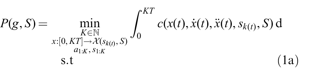
The complete LGP formulation (1), however, not only seeks to find a feasible solution, but also an action sequence that leads to the minimum trajectory costs (1a) compared with all other goal reaching sequences. We call a feasible solution a solution to the TAMP/LGP problem, whereas we call a solution that minimizes the cost an optimal solution of the LGP. Owing to the vast number of possible discrete action sequences, obtaining optimal solutions is often intractable. Therefore, we mostly focus on obtaining a feasible solution, with the exception of Sections 4.8 and 5.3.7.
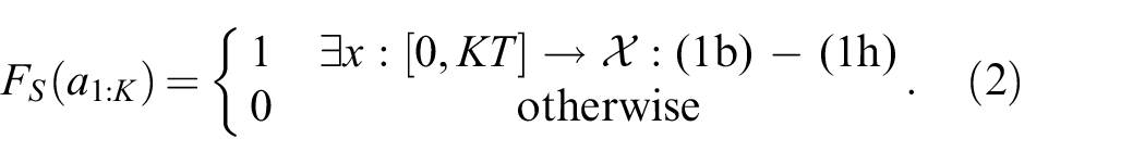
The feasibility as defined in (2) is a theoretical property of the resulting nonlinear program. In practice, we solve (1) numerically by discretizing
3.2. Multi-bound LGP tree search and lower bounds
The logic induces a decision tree (called LGP tree) through the set of possible actions
More specifically, multi-bound LGP tree search uses two lower bounds
As we show in the experiments, even with those bounds, a large number of NLPs have to be solved to find a feasible solution for problems with a high combinatorial complexity. Therefore, using these bounds is not sufficient to achieve desirable solution times for the problems we consider in the experiments. This is especially true if many decisions are feasible in early phases of the sequence, but then later become infeasible, because then the lower bounds do not help much in pruning the search tree. These lower bounds are, however, highly important to make the data generation process tractable.
4. Deep visual reasoning
The central idea of this work is, given the scene and the task goal as input, to predict a promising discrete action sequence
We first describe more precisely what should be predicted, then how the scene, i.e., the objects and actions that operate on them, and the goal can be encoded as input to a neural network that should perform the prediction. Finally, we discuss how the network is integrated into the tree search algorithm in a way that either directly predicts a feasible sequence or, in case the network is mistaken, acts as a search heuristic to further guide the search without losing completeness, i.e., the ability to find a solution if one exists. To allow for a more thorough comparison, we additionally propose an alternative way to integrate learning into LGP based on a goal-independent recurrent feasibility classifier.
4.1. Predicting promising action sequences
First, we define for the goal
In relation to the LGP tree, this is the set of all leaf nodes and, hence, candidates for an overall feasible solution. One idea is to learn a discriminative model which predicts whether a complete sequence leads to a feasible NLP and, hence, to a solution. To predict an action sequence one would then choose the sequence from
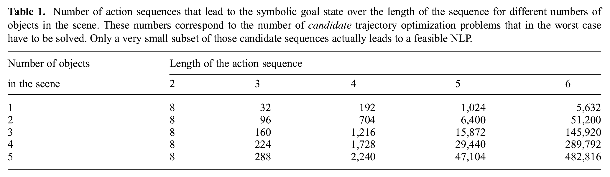
Number of action sequences that lead to the symbolic goal state over the length of the sequence for different numbers of objects in the scene. These numbers correspond to the number of candidate trajectory optimization problems that in the worst case have to be solved. Only a very small subset of those candidate sequences actually leads to a feasible NLP.
Instead, we propose to learn a function
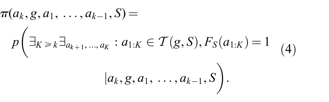
Note that this includes
In this way, we can utilize
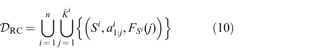
4.2. Training targets
The crucial question arises how
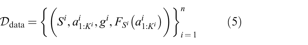
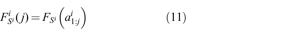
where the feasibility
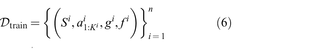
where
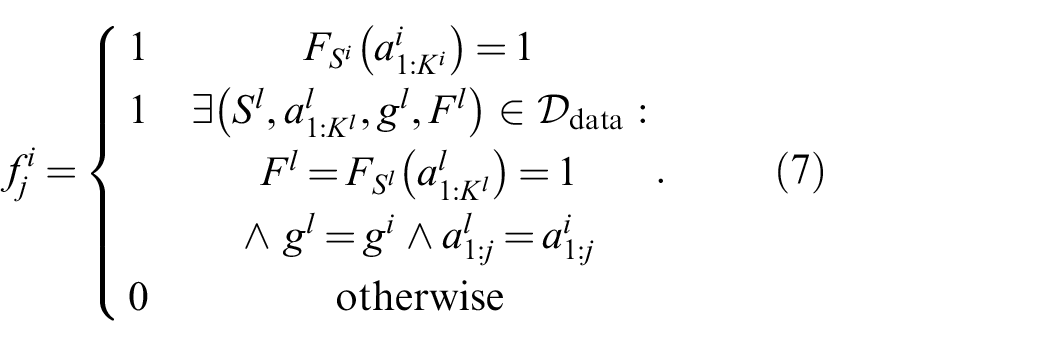
Superscripts denote dataset indexing. If the action sequence is feasible and solves the problem specified by
4.3. Input to the neural network: encoding
,
, and
So far, we have formulated the predictor
4.3.1. Splitting actions into action operator symbols and objects
An action
Specifically, given an action
The cardinality of
4.3.2. Encoding the objects
and
in the image space
For our approach it is crucial to encode the information about the objects in the scene in a way that allows the neural network to generalize over objects, i.e., the number of objects in the scene and their properties. By using the separation of the last paragraph, we can introduce the mapping
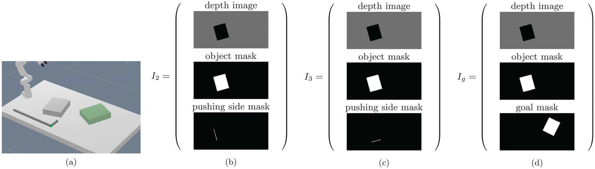
In Figure 1, we show these image encodings for a scene of the pick-and-place experiment. Figures 1(b) and (c) show action–object images, whereas Figure 1d shows the goal-image encoding.
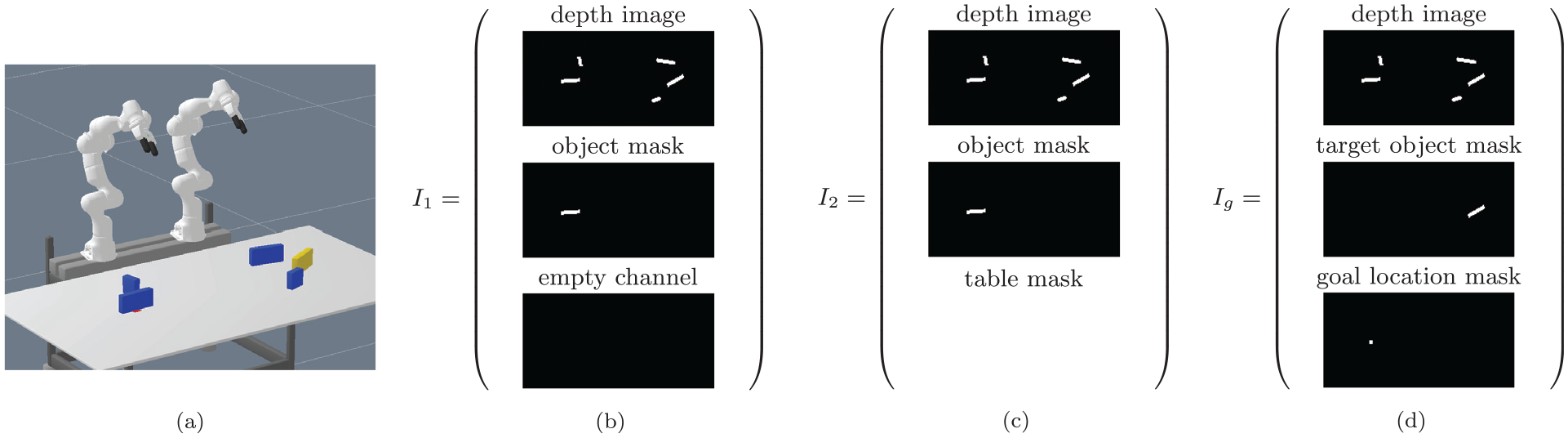
Visualization of the action–object image encodings
It is important to understand that
Please note that these action–object images always correspond to the initial scene.
4.4. Network architecture
Figure 2 shows the network architecture that represents
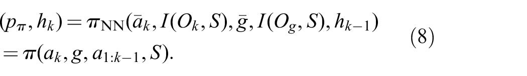
Proposed neural network architecture.
4.5. Relation to
-functions and offline RL
In principle, one can view the way we define
However, we want to clarify that the decision process
Therefore, the
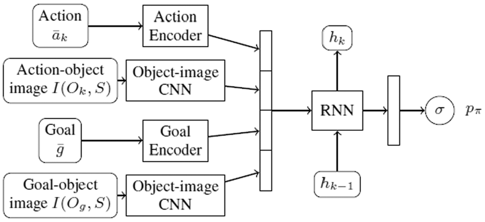
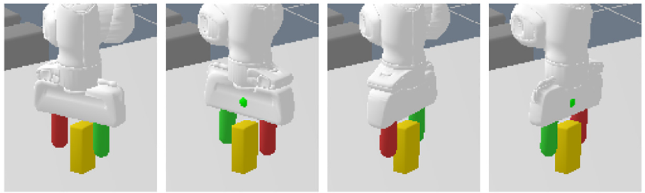
To illustrate that, we show in Figure 3 the fact that future discrete actions can change the resulting optimized trajectory in earlier motion phases.
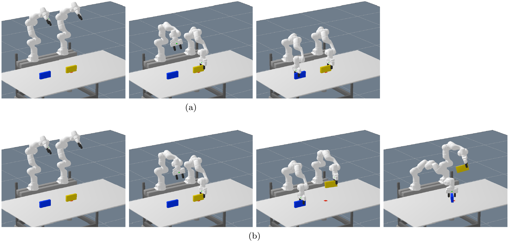
Illustration that the behavior of the optimized trajectory is only fully defined for a complete sequence of discrete actions. (a) Action sequence grasp(R
This raises the question which state/action representation is appropriate for learning such a
We propose the action–object image sequence as a powerful input representation for such a
Furthermore, it is difficult to encode the symbolic state as an input, especially for multiple objects. Therefore, we implicitly encode the state via the sequence (or history) of actions. This is not only sufficient, because a sequence of actions uniquely determines the symbolic state sequence, but advantageous, because actions explicitly only depend on a small subset of objects, as compared with the complete symbolic state. However, as discussed previously, the actions also require the complete initial scene information, which is provided in terms of the image of the whole scene. The fact that the action–object images contain geometry information of the scene couples the abstract symbolic level to the concrete scene instance, making the reasoning process possible.
In summary, our network has to learn a state representation for the abstract decision process from the past action–object image sequence, while only observing the initial state in form of the depth image of the scene as input, conditioned on the goal.
Through the data transformation (7), we can frame learning
4.6. Algorithm
Algorithm 1 presents the pseudocode of how
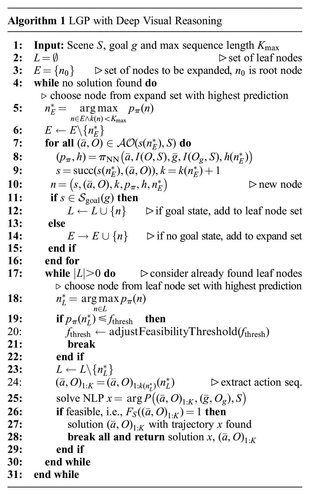
The main idea of the algorithm is to maintain the set
At each iteration, the algorithm chooses the node
If a child node reaches a symbolic goal state (line 11), it is added to the set of leaf nodes
Then those already found leaf nodes from the set
4.6.1. Feasibility threshold and completeness of the algorithm
As during the expansion of the tree, leaf nodes which are unlikely to be feasible are also found, only those trajectory optimization problems are solved where the prediction
This greatly reduces the number of NLPs that have to be solved, because the information provided by the network is not only used to guide the tree search to find promising leaf nodes quickly, but also to discard leaf nodes that are predicted to be infeasible by the network.
However, one cannot expect that the network never erroneously has a low prediction although a leaf node would be feasible. In order to prevent not finding a feasible solution in such cases, the function
Proof. Clear by construction of Algorithm 1 and the feasibility threshold discounting through
This means that if a scene contains at least one action sequence that reaches the symbolic goal for which the nonlinear trajectory optimizer can find a feasible motion, Algorithm 1 finds this solution. In particular, the neural network does not prevent finding a solution, even in case of prediction errors. Another way to interpret Proposition 1 is that the network
In Assumption 1 we assumed a maximum sequence length
If we set
4.6.2. Implementation
As an important remark, for the implementation we store the hidden state of the RNN in its corresponding node. Furthermore, the action–object images and action encodings also have to be computed only once, because all action–object images correspond to the initial scene configuration. Therefore, during the tree search, only one pass of the recurrent (and smaller) part of the complete
4.7. Comparative alternative: goal-independent recurrent feasibility classifier
The methods of Driess et al. (2020b) and Wells et al. (2019) learn a feasibility classifier for single actions only, i.e., independent of a goal, and do not consider sequences. To allow for a comparison, we present in this section an approach to extend the idea of a feasibility classifier to action sequences and how it can be integrated into our TAMP framework.
The basic idea is to classify the feasibility of a motion planning problem that results from an action sequence with a recurrent classifier, independently from and agnostic to a goal. In this way, during the tree search, solving an NLP as a lower bound to guide the search can be replaced by evaluating the classifier, which usually is order of magnitudes faster. Formally, we seek to learn a function that, given a scene description

This is independent from the overall goal of the TAMP problem. Instead,
Regarding the dataset for training such a classifier, assume that we have sampled a scene
with
where
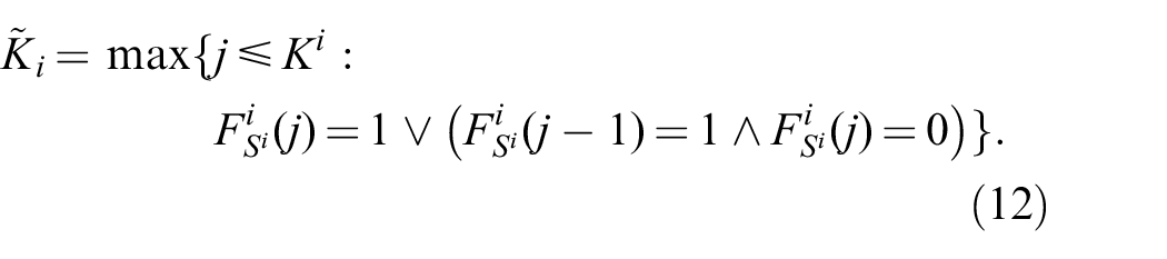
Superscripts here denote dataset indexing. For the actual implementation, we basically choose the same architecture as for
Section 5.2.6 presents an empirical comparison of this recurrent classifier with the goal-conditioned predictor
4.8. Predicting trajectory cost
So far, we were only interested in finding a feasible action sequence. The full LGP formulation (1), however, seeks not only for feasibility, but also optimality with respect to the trajectory costs measured by the function
However, for the more dynamic pushing experiment of Section 5.3, there can be more significant differences in the trajectory costs even for action sequences of the same sequence length. Therefore, we present in this section a simple modification of the network and especially the training targets to enable the network to predict the expected trajectory cost for an action sequence. This way, we can utilize the network to find more cost optimal solutions compared to the case where we only take feasibility into account.
Let
The training targets of the
If there exists no future feasible action sequence when taking
Analogously to the discussion in Section 4.5, the role of
When integrating
5. Experiments
We demonstrate our proposed framework on two different tasks. Please also refer to Extension 1 that demonstrates the planned motions both in simulation and with a real robot.
For the first experiment, presented in Section 5.2, we consider a typical kinematic pick-and-place TAMP problem where two robot arms have to collaborate to solve the tasks. We investigate the generalization capabilities of our approach to more objects in the environment than during training.
In the second experiment (Section 5.3), we show that the method can also be applied to tasks that involve dynamic models. More specifically, we demonstrate a tool-use scenario where the robot has to use a hook-shaped object to push and/or pull an object to a desired target location.
As a general remark, the quantitative results are visualized using boxplots that show the median, the upper and lower quartiles as well as whiskers. The whiskers in all boxplots correspond to datapoints that are nearest to 1.5 times the interquartile range (IQR). When we obtained time measurements, we ensured to run them on the same machine which did not compute anything else at the time. All experiments in Section 5.2 that report run times have been performed with an Intel Xeon W-2145 CPU @ 3.70 GHz, whereas in Section 5.3 they were run with an Intel Xeon E5-2630v4 CPU @ 2.20 GHz.
5.1. Network details
Both experiments share the same network architecture with the same hyperparameters. The network is trained with the ADAM optimizer (learning rate 0.0005) with a batch size of 48 for the pick-and-place experiment and 40 for the pushing experiment. To account for the aforementioned imbalance in the dataset, we oversample feasible action sequences such that at least 16 out of the 48 samples in one batch come from a feasible sequence for the pick-and-place experiment (8 out of 40 for the pushing one). More specifically, 32 are sampled without replacement from the whole dataset, whereas the additional 16 (or 8) are solely sampled from the feasible ones with replacement. We additionally weight the feasible samples in the loss function with a weight of 2. In general, accounting for the imbalance with this oversampling turned out to be crucial for the performance. However, there was no extensive tuning of hyperparameters necessary at all.
The image encoder consists of three convolutional layers with 5, 10, and 10 channels, respectively, and filter size of
5.2. Pick-and-place experiment
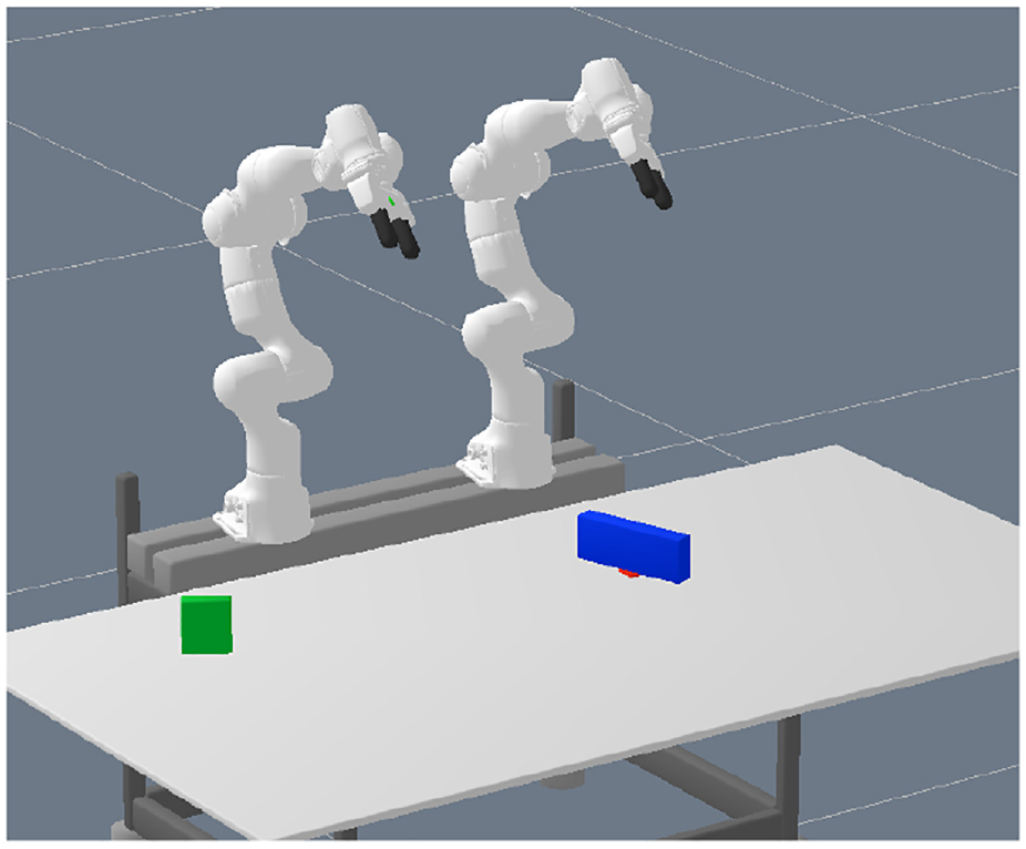
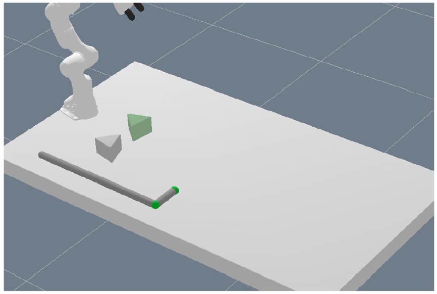
For the first experiment, we consider a tabletop scenario with two robot arms (Franka Emika Panda) and multiple box-shaped objects, see Figure 1a, 4, or 5 for typical scenes, in which the goal is to move an object to different target locations. The target locations are visualized by red squares in these figures.
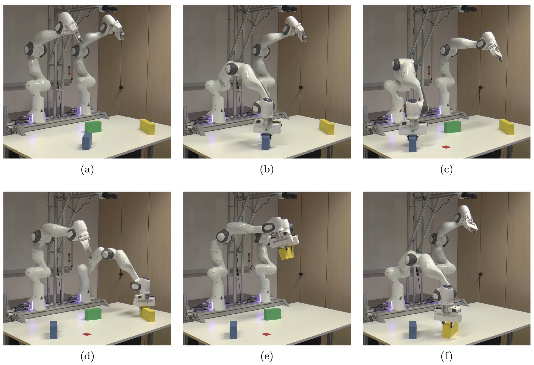
Typical scene of the pick-and-place experiment: (a) initial scene from which the image is captured; (b) action 1 (grasp), remove occupying object; (c) action 2 (place); (d) action 3 (grasp); (e) action 4 (grasp), handover; (f) action 5 (place), goal achieved. The yellow object should be placed on the red spot, which is, however, occupied by the blue object. Furthermore, the yellow object cannot be reached by the robot arm that is able to place it on the red spot. Therefore, the two arms have to collaborate to solve the task. In this case, the network decides for a handover solution.
Training scene example of the pick-and-place experiment. The sizes, positions, and orientations of the two boxes as well as the target location (red spot) are sampled randomly. Here the green box should be placed on the red spot.
5.2.1. Action operators and optimization objectives
The logic language is defined by rules similar to PDDL (Planning Domain Definition Language). For the pick-and-place experiment, there are two action operators
The
The four different integer assignments of the
Note that the exact grasping location in two degrees of freedom relative to the object is not defined completely by the
Finally, the
The
Preconditions for
Path costs
In total,
5.2.2. Properties of the scene
There are multiple properties which make this (intuitively simple) task challenging for TAMP algorithms. First, the target location can fully or partially be occupied by another object. Second, the object and/or the target location can be out of reach for one of the robot arms. Hence, the algorithm has to figure out which robot arm to use at which phase of the plan and the two robot arms possibly have to collaborate to solve the task. Third, apart from position and orientation, the objects vary in size, which also influences the ability to reach or place an object. In addition, grasping box-shaped objects introduces a combinatorics that is not handled well by nonlinear trajectory optimization due to local minima and also joint limits. Therefore, as described in the last paragraph, we introduce integers as part of the discrete action that influence the grasping geometry. This greatly increases the branching factor of the task. For example, depending on the size of the object, it has to be grasped differently or a handover between the two arms is possible or not, which has a significant influence on the feasibility of action sequences.
Indeed, Table 1 lists the number of action sequences with a certain length that lead to a symbolic goal state over the number of objects in the scene. This number corresponds to candidate sequences for a feasible solution (the set
One could argue that an occupied and reachability predicate could be introduced in the logic to reduce the branching of the tree. However, this requires a reasoning engine which decides those predicates for a given scene, which is not trivial for general cases. More importantly, both reachability and occupation by another object is something that is also dependent on the geometry of the object that should be grasped or placed and, hence, not something that can be precomputed in all cases (Driess et al., 2020b, 2019b). For example, if the object that is occupying the target location is small and the object that should be placed there as well, then it can be placed directly, whereas a larger object that should be placed requires to first remove the occupying object. Our algorithm does not rely on such non-general simplifications, but decides promising action sequences based on the real relational geometry of the scene, encoded in the action–object images and the goal image.
5.2.3. Training/test data generation
We generated 30,000 scenes randomly with two objects present at a time. The sizes, positions, and orientations of the objects as well as the target location are sampled uniformly within a certain range. In total, the parameter scene space is 14-dimensional. See Figure 5 for an example of a typical training scene. For half of the scenes, one of the objects (not the one that is part of the goal) is placed directly on the target, to ensure that at least half of the scenes contain a situation where the target location is occupied. The dataset
To evaluate the performance and accuracy of our method, we sampled 3,000 scenes, again containing 2 objects each, with the same algorithm as for the training data, but with a different random seed. Using breadth-first search, we determined 2,705 feasible scenes, which serve as the actual test scenes.
5.2.4. Performance: results on test scenarios
This section presents the performance of our network when integrated into the tree search algorithm to find solutions for the 2,705 test scenarios that contain 2 objects each.
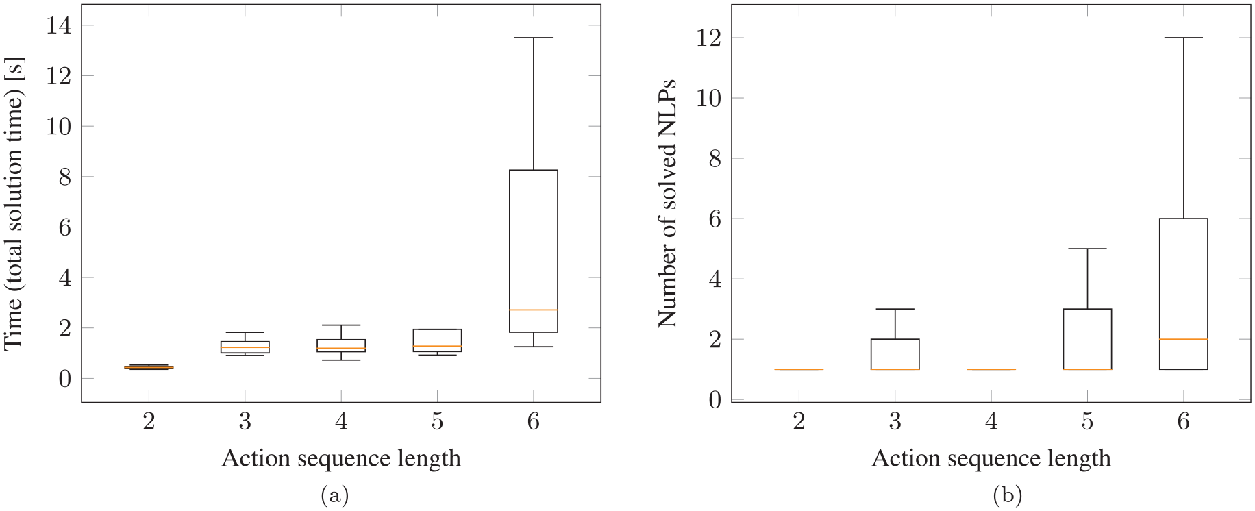
Figure 7 shows both the total runtime and the number of NLPs that have to be solved to find a feasible solution. When we report the total runtime, we refer to everything, meaning capturing the image, computing the image/action encodings, querying the neural network during the search and the time for all involved NLPs that are solved. As one can see in Figure 7b, for all cases with sequence lengths of 2 and 3, the first predicted action sequence is feasible, such that there is no search necessary and only one single NLP has to be solved. For length 3, the median is still 1, but also for sequences of lengths 5 and 6 in half of the cases less than 2 NLPs have to be solved.
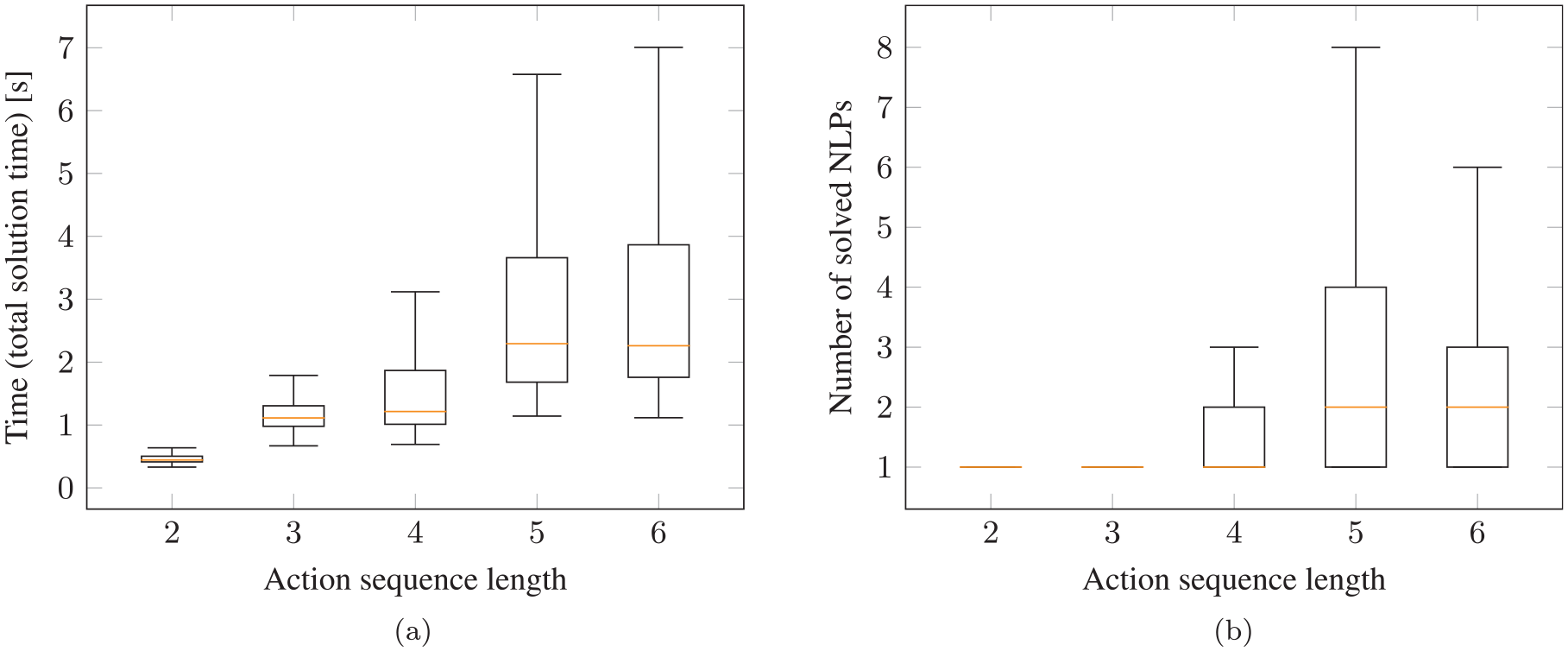
Performance on test scenarios for pick-and-place experiment (two objects in the scene) with neural network integrated into the tree search algorithm: (a) total time to find a feasible solution; (b) number of NLPs that have to be solved to find a solution. As can be seen in (b), in many cases only a single NLP has to be solved or 2 (median) for more challenging tasks that require action sequence lengths of 5 and 6.
In general, with a median runtime of about 2.3 s for even sequence length of 6, the overall framework with the neural network has a high performance and the task can be solved in reasonable runtime. Furthermore, the upper whiskers are also below 7 s.
Of the 2,705 test scenes, in 35% of the cases the network finds a solution with sequence length 2, in 18% of length 3, in 27% of length 4, in 7% of length 5, and in 13% of length 6. Therefore, it is important that we report the runtimes and the number of solved NLPs separated as a function of the sequence length. Otherwise, the simpler cases of sequence length 2 and 3, where there is a smaller combinatorial complexity, would cover 53% of all test scenarios. This allows us to show that also for the harder cases of sequence length 5 and 6, which are only 20% of the test scenes, the network performs well.
5.2.5. Comparison with multi-bound LGP tree search
Here we compare the performance of multi-bound LGP tree search that utilizes the lower bounds from Toussaint and Lopes (2017) as heuristics to guide the search with our proposed framework where the network acts as a heuristic or ideally directly predicts a feasible action sequence.
In Figure 8a the runtimes for solving the test cases with LGP tree search are presented, which shows the difficulty of the task. In 132 out of the 2,705 test cases, LGP tree search is not able to find a solution within the timeout, compared with only 3 times when we use our proposed framework with the neural network.
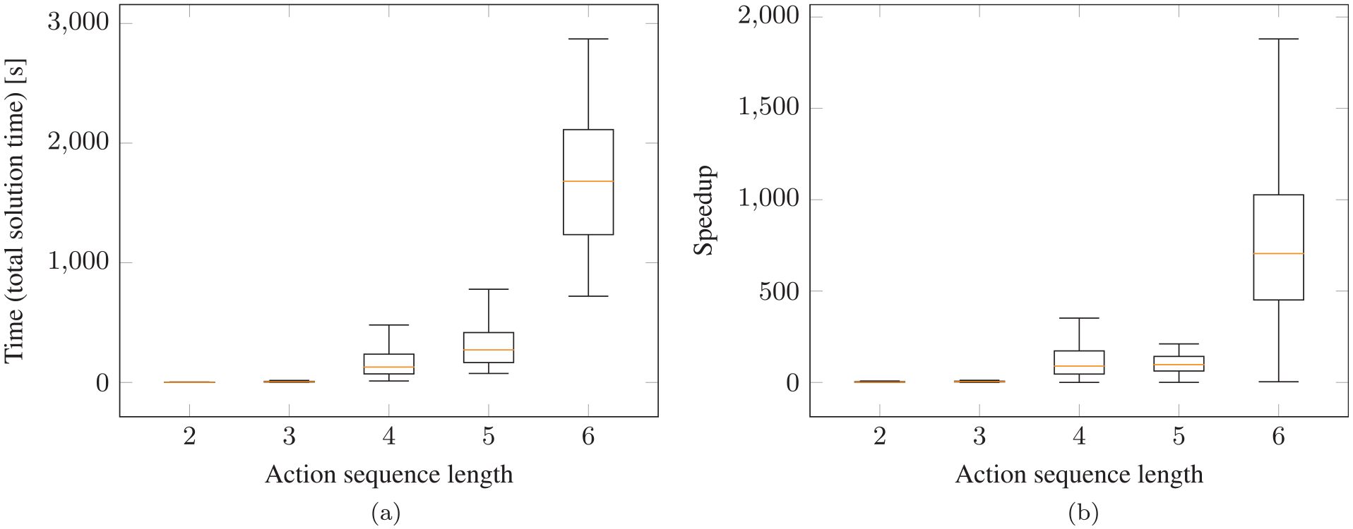
Comparison of our framework with the neural network to multi-bound LGP tree search that relies on computing lower bounds to guide the search: (a) total time with LGP to find a feasible solution; (b) speedup gained when using our proposed network over multi-bound LGP tree search. The speedup in (b) is the solution time with multi-bound LGP tree search divided by the solution time with the neural network. Test scenes of pick-and-place experiment with two objects in the scene.
Figure 8b shows the speedup that is gained by using the neural network. For sequence length 4, the network is 46 times faster, 100 times for length 5, and for length 6 even 705 times faster (median). In this plot, only those scenes where LGP tree search and the neural network have found solutions with the same sequence lengths are compared, which is the case in 78% of the test scenes. This means that especially for the difficult cases, where it is most relevant, utilizing the network also leads to a significant speedup.
5.2.6. Comparison with the recurrent classifier
Figure 9a shows a comparison of our proposed goal-conditioned network that generates sequences with the recurrent classifier described in Section 4.7 that only predicts the feasibility of an action sequence, independent from the task goal. As one can see, although such a classifier also leads to a significant speedup compared with LGP tree search, our goal-conditioned network has an even higher speedup, which also stays relatively constant with respect to increasing action sequence lengths. Furthermore, with the classifier 22 solutions have not been found, compared with 3 with our approach within the timeout. Although the network query time is neglectable for our network, as can be seen in Figure 9b, the time to query the recurrent classifier becomes visible. Indeed, one can see the exponential increase in the network query time for increasing sequence lengths. This is caused by the fact that without goal conditioning, the network has to be queried much more often, because it can only assess the feasibility of an action sequence up to the point it has been queried without the ability to judge whether it eventually leads to the goal. Therefore, the speedup compared with LGP tree search with the recurrent classifier is achieved by replacing the analytically defined lower bounds which can, especially if the problem is infeasible, take up to several seconds to compute, with a learned model acting as a lower bound that is not only much faster to evaluate, but also has a constant query time. The goal conditioning of our proposed framework does not show this exponential increase for longer sequence lengths, because it directly guides the search towards achieving the goal.
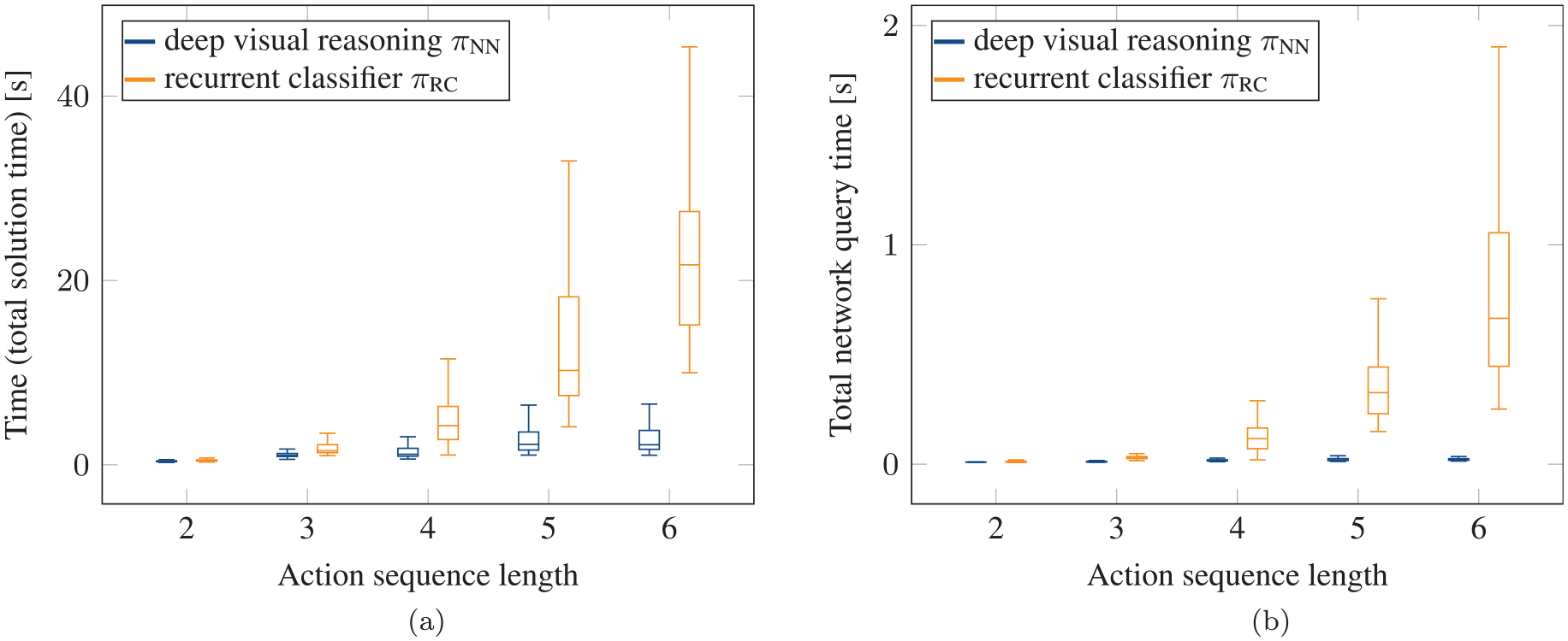
Comparison of recurrent classifier (orange) to our proposed goal-conditioned network (blue) for pick-and-place experiment on test scenes with two objects in the scene: (a) total time to find a feasible solution with recurrent classifier; (b) total, i.e., summed up, time to query the networks to find a solution for a scene (part of the total solution time of (a)). Although the recurrent classifier is competitive compared to LGP tree search (see Figure 8a), one can see the exponential increase in the runtime for longer sequence lengths. In contrast, the runtime with our proposed framework increases much less for longer sequence lengths.
5.2.7. Data efficiency
One could argue that the 25,736 scenes used for training are a high number of scenes for this task. However, one also has to take into account that the parameter space from which the scenes are sampled is 14-dimensional, which means that the training set does not cover this space densely at all. Nevertheless, we trained our proposed network on a subset of 4,442 and 8,090 scenes of the original training dataset. In Figure 10, we report the number of solved NLPs to find a solution for the networks that are trained on 4,442, 8,090, and 25,736 scenes, split over the length of the found action sequence. As one can see, the median is the same for all networks. For longer sequence lengths of 5 and 6, the upper quartiles and the upper whiskers for the networks trained on the smaller datasets increase. Nevertheless, this experiment shows that with nearly six times less data, one still achieves a high performance, which is also still orders of magnitudes better than without the network.
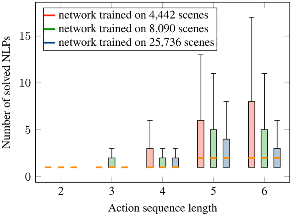
Investigation of the data efficiency. Number of solved NLPs to find an overall feasible solution for the test scenes with neural network integrated into the tree search algorithm for networks trained on different numbers of training scenes. Pick-and-place experiment. The median is the same for all networks.
5.2.8. Feasibility threshold and completeness
In Section 4.6, we have discussed how the network can be integrated into the tree search algorithm without preventing a solution being found if one exists even in case of prediction errors of the network. This is achieved by adjusting the feasibility threshold with a discounting factor
Figure 11 shows the total solution time to find a feasible solution with the network when using the feasibility threshold together with the adjustment of the threshold (blue), which is our proposed approach, the case without the adjustment (red), which implies that solutions can be missed in case of prediction errors, and the case where there is no threshold at all (green).
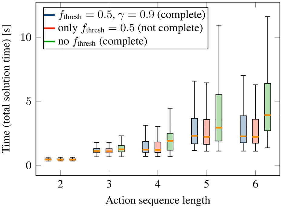
Performance on test scenarios depending on the feasibility threshold strategy for the pick-and-place experiment (two objects in the scene) with neural network integrated into the tree search algorithm. Blue is our proposed approach that combines the advantages of using the feasibility threshold for performance while maintaining completeness.
As can be seen, the case without the threshold has the highest runtime, whereas the case with the threshold but no discounting has the lowest runtime. However, our proposed approach with the threshold and the discounting (blue) has only a non-significant difference to the case with threshold but no discounting. Even without the threshold, the performance is also very good, although clearly worse than with our proposed approach.
As we discussed in Proposition 1, the approach with adjusting the feasibility threshold guarantees that a solution can be found if it exists. Indeed, in only 3 of the 2,705 test cases, no solution was found with this method within the timeout. The fact that this number is not zero is due to the timeout. If we increase the timeout, then indeed a solution for all test cases was found. The same holds true for the case without the threshold, i.e., for the initial timeout 3 were not found, then with the increased timeout all were. However, even if we increased the timeout, still in 5 test cases no solution was found when using the threshold without the adjustment mechanism.
For the networks that have been trained on a smaller dataset (Section 5.2.7), adjusting the feasibility threshold turned out to be even more important. Without the feasibility adjustment, the network trained on 4,442 (8,090) scenes did not find a solution in 30 (17) cases. In contrast, with the feasibility adjustment, the networks trained on the smaller datasets did not find a solution in only 2 (1) cases. When increasing the timeout, always a solution was found in the latter case.
To summarize, the feasibility threshold adjustment presented in Section 4.6.1 maintains completeness, while showing very little performance penalty.
The threshold in the experiments was
5.2.9. Generalization to multiple objects
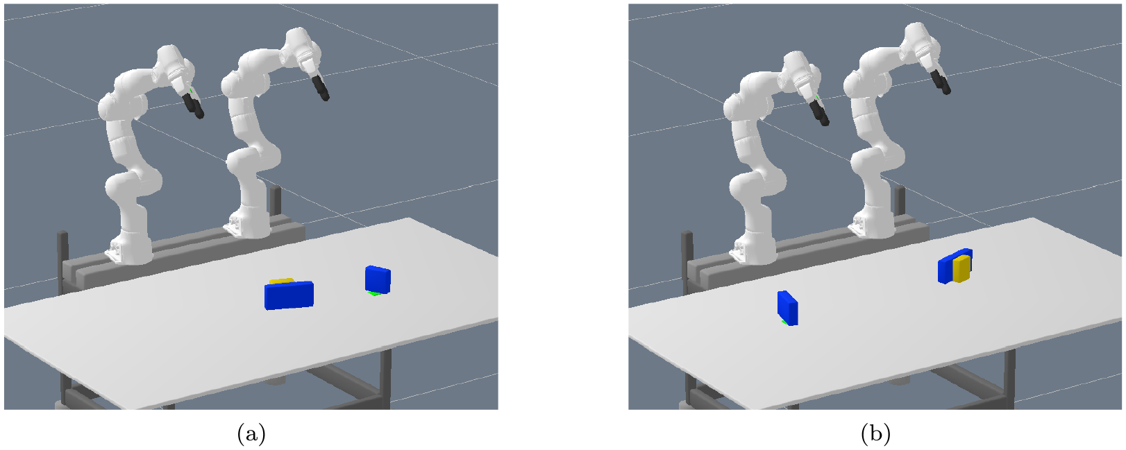
Creating a rich enough dataset containing combinations of different numbers of objects is infeasible. Instead, we now take the network that has been trained as described in Section 5.2.3 with only two objects present at a time and test whether it generalizes to scenes with more than two (and also only one) objects. The 200 test scenes are always the same, but more and more objects are added. In Figure 1a and 12, such test scenes with 4 and 5 objects are shown.
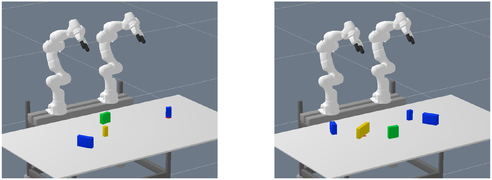
Example scenes for generalization to multiple objects (pick and place experiment). Object colors have no meaning.
Figure 13 reports the total runtime to find a feasible solution with our proposed neural network over the number of objects present in the scene. These runtimes include all scenes with different action sequence lengths. In all cases a solution was found. Although the upper quartile increases, the median is not significantly affected by the presence of multiple objects.
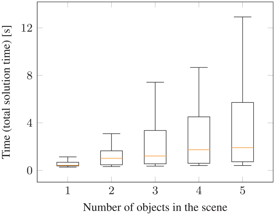
Generalization to multiple objects for pick-and-place experiment with the proposed deep visual reasoning neural network. During training, only and exactly two objects have been present in the training scenes. Although the number of candidate action sequences increases exponentially with more objects in the scene (see Table 1), the runtime to find a feasible solution with the neural network increases only slightly when more objects are added.
The observation that the runtime increases for more objects is not only caused by the fact that the network inevitable makes some mistakes and, hence, more NLPs have to be solved. Solving (even a feasible) NLP with more objects can take more time due to increased runtime costs for collision queries and increased non-convexity of the optimization landscape.
In general, the performance is remarkable, especially when observing that the network was able to find solutions for scenes with many objects in a reasonable amount of time for sequence length 6, where, according to Table 1, nearly half a million possible action sequences for 5 objects in the scene exist.
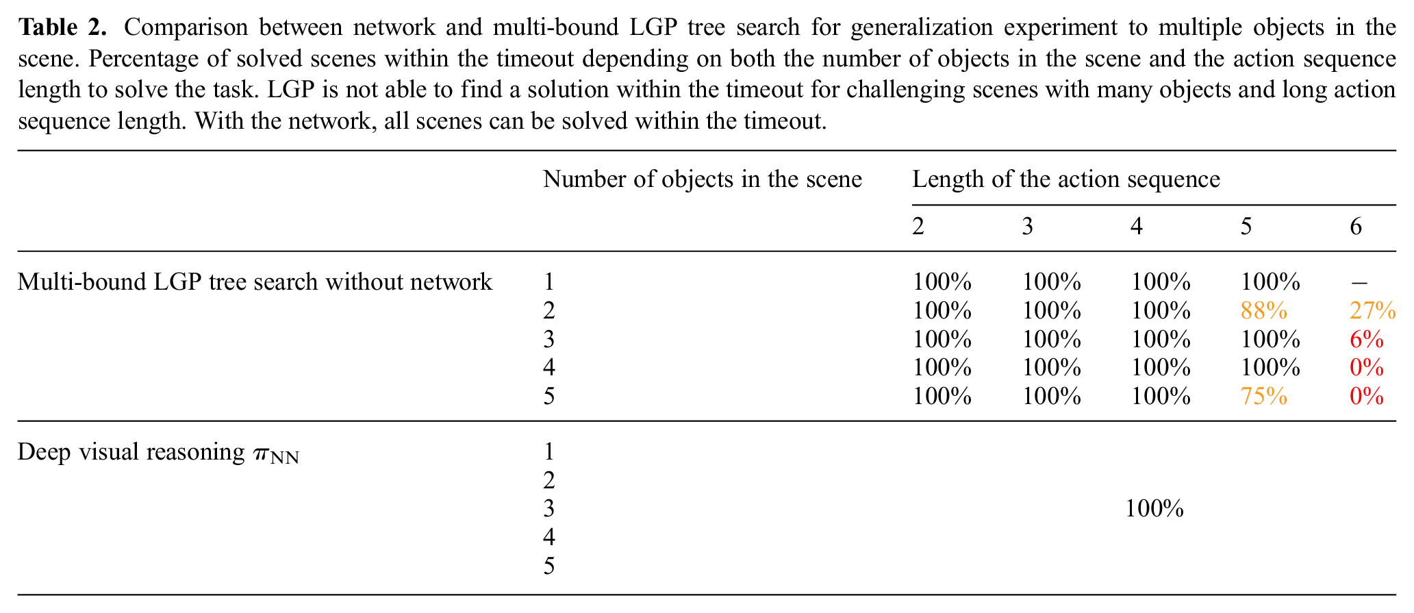
To further demonstrate the advantages of the network when generalizing to multiple objects, in Figure 14, we compare the proposed approach to multi-bound LGP tree search. We split the evaluation between scenes that have been solved with action sequence lengths of 2 or 3 (Figure 14a) and 4, 5, or 6 (Figure 14b). For the more challenging scenes requiring sequence lengths 4, 5, or 6, the runtime is between 2 and 3 orders of magnitudes smaller with the network. Note that the runtimes in Figure 14 for LGP are only reported for those where LGP was able to find a solution within the timeout. As indicated in Table 2, for the challenging scenes that require action sequence length 6, if the scene contains 3 objects, then in only 6% of the cases the network was able to find a solution within the timeout. If the scene contains 4 or 5 objects, then LGP without the network was not able to solve a single scene within the timeout. Therefore, the runtime results in Figure 13 are in favor of LGP. As mentioned, with our proposed approach, in all cases a solution was found.
Comparison between network and multi-bound LGP tree search for generalization experiment to multiple objects in the scene. Percentage of solved scenes within the timeout depending on both the number of objects in the scene and the action sequence length to solve the task. LGP is not able to find a solution within the timeout for challenging scenes with many objects and long action sequence length. With the network, all scenes can be solved within the timeout.
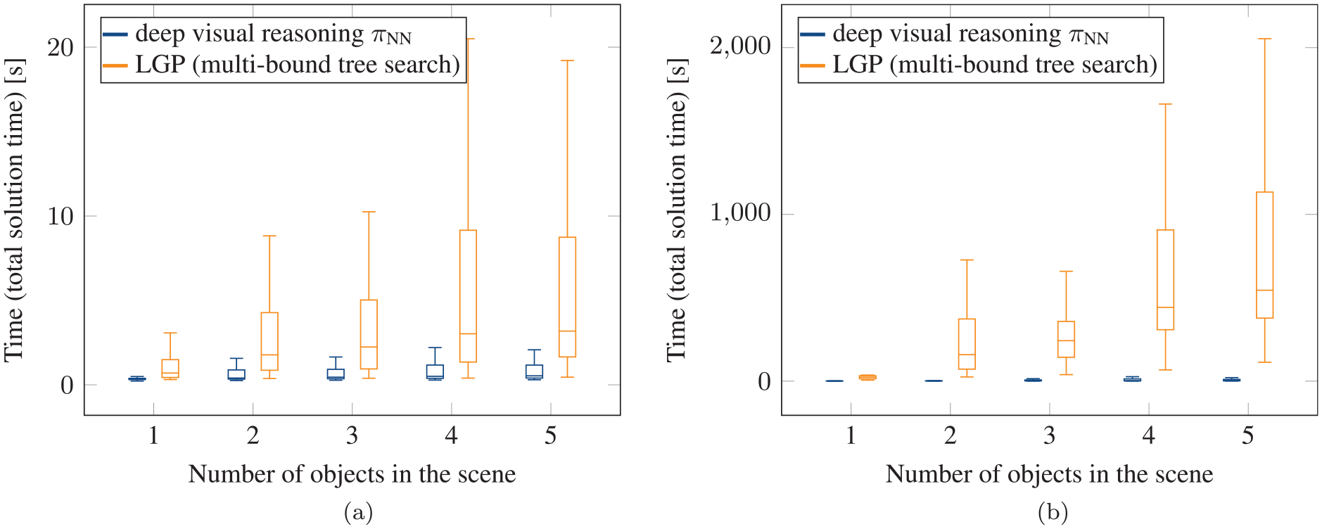
Comparison with multi-bound LGP tree search for the generalization to multiple objects experiment (pick-and-place scenario). Plots show the total runtime to find a feasible solution, split over scenes that could be solved with (a) an action sequence length of 2 or 3 and (b) an action sequence length 4, 5, or 6. The results show that the increased number of candidate action sequences for more objects in the scene (Table 1) leads to significantly longer solution times for LGP. In contrast, the runtime to find a feasible solution with the neural network increases only slightly when more objects are added.
These results emphasize that the capability of the network to reason about which objects are relevant to solve the task is crucial, even if only two objects have to be manipulated. Therefore, the network shows important generalization capabilities to multiple objects.
5.2.10. Generalization to more objects to be manipulated and longer sequence lengths
In the last section, we have shown that the network is able to generalize to more objects in the scene than it has been trained on. In those scenes, it was, however, sufficient to manipulate two objects to solve the task, as in the training distribution. As increasing the number of objects in the scene increases the number of candidate action sequences significantly, determining the relevant objects is, as we have shown, an important capability of the network to maintain high performance when generalizing to multiple objects.
Going beyond that, the question arises if the network is also useful in situations where more than two objects have to be manipulated to solve the task. We do not expect the network to generalize to these settings with the same performance as in the other experiments.
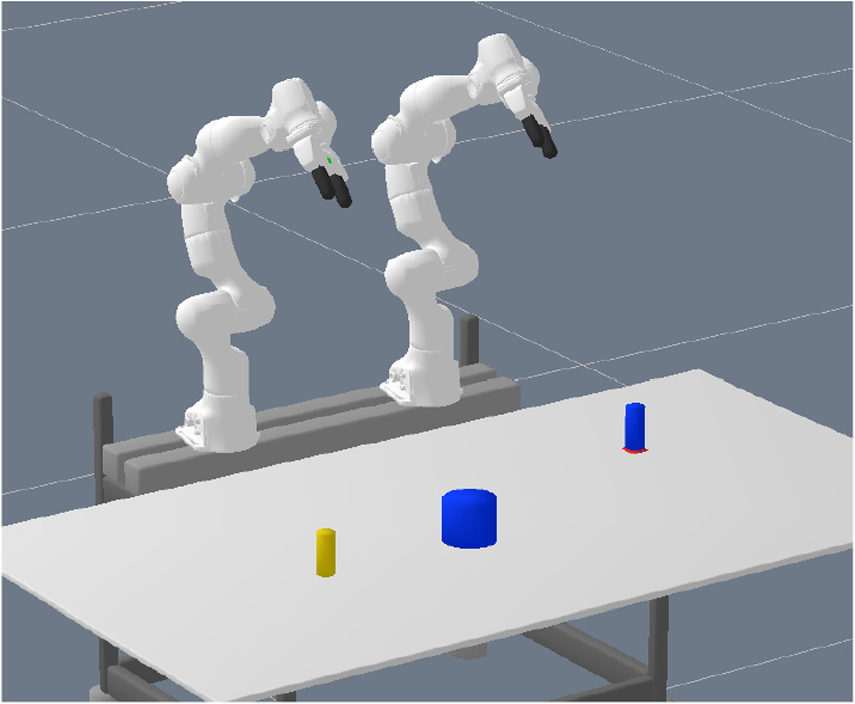
In order to investigate this question, we generated five test scenes where not only the goal is obstructed by an object, but also the target object that should be placed on the goal cannot be grasped directly because another object is placed in a way that prevents grasping. See Figure 15a for an example scene. We call this experiment 1 in the following. This means that all three objects have to be manipulated to solve the task. Further, we generated three test scenes (see Figure 15b for an example) where, more challenging, the objects are placed in a way such that at least eight discrete actions are necessary due to the reachable set of the robot arms (and, hence, they have to collaborate). We call this experiment 2 in the following. These numbers of test scenes are not as statistically significant as the evaluations presented in the other parts of this work. This is due to the fact that randomly sampling scenes where three objects have to be manipulated is unlikely given our data-generation method. Therefore, we created these test scenes manually, without any bias to their solvability for the method.
Generalization experiment where three objects have to be manipulated to solve the task, because not only is grasping the target object (yellow) obstructed by another object, but the goal location is also occupied with yet another object: (a) minimum required sequence length 5 or 6; (b) minimum required sequence length 8. The training distribution contained scenes with two objects only. Hence, only a maximum of two objects within an action sequence length of up to 6 have to be manipulated. Therefore, for the scene in (b), we ask for generalization in two ways beyond the training distribution, namely three objects to be manipulated and longer sequence length.
Table 3 presents the runtimes for this generalization experiment for all scenes individually. We increased the timeout by a factor of 10 for this experiment compared with the others. Out of the five scenes for experiment 1, in four cases a solution was found using our network within the timeout. LGP was also able to find a solution for these four cases. Regarding experiment 2, in all three test scenes a solution was found with our network, whereas LGP was not able to find a solution for two of the three cases.
Runtime results for generalization experiment where three objects have to be manipulated to solve the task
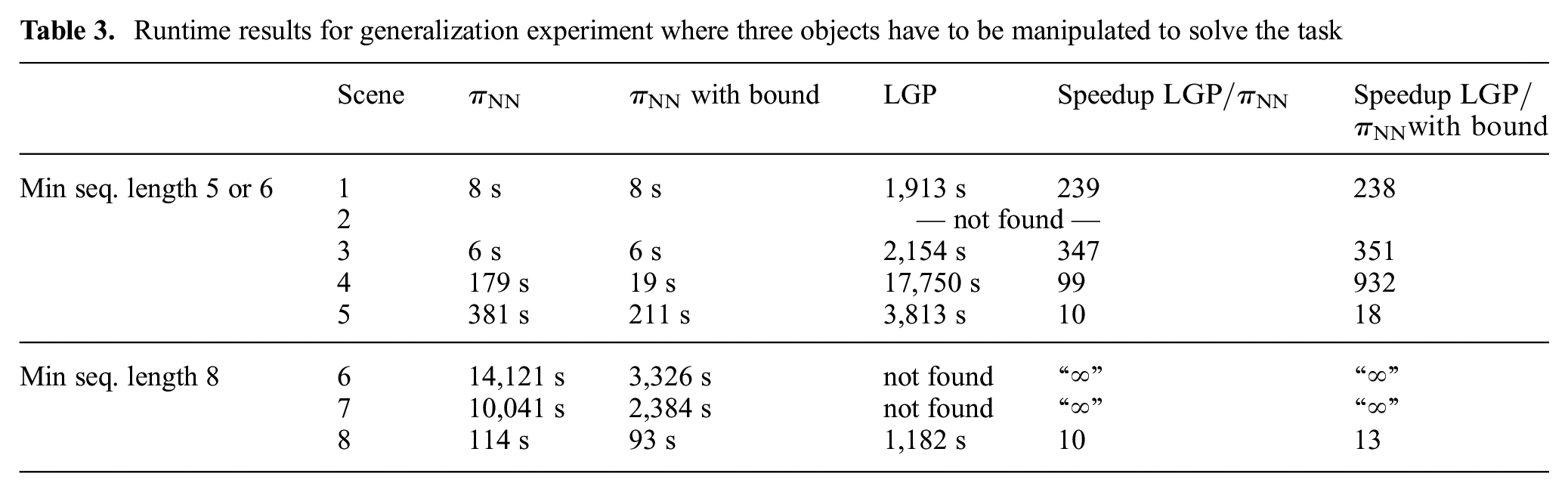
Although the network for these scenes cannot reduce the number of optimization problems that have to be solved as much as in the other experiments, in comparison with LGP, the speedup between 10 and 932 is still remarkable and the network makes it possible to solve some scenes at all. There are scenes where the task could be solved in less than 10 s with the network, but others can take of the order of hours. Therefore, the network acts as a heuristic to speed up the search, but does not eliminate it.
The column “
5.2.11. Generalization to cylinders
Although the network has been trained on box-shaped objects only, we investigate whether the same network can generalize to scenes which contain other shapes such as cylinders. As the objects are encoded in the image space, there is a chance that, as compared with a feature space which depends on a less-general parameterization of the shape, this is possible. We generated 200 test scenes that either contain two cylinders, three cylinders or a mixture of a box and a cylinder, all of different sizes/positions/orientations and targets. If the goal is to place a cylinder on the target, we made sure in the data generation that the cylinder has an upper limit on its radius in order to be graspable. These cylinders, however, have a relatively similar appearance in the rasterized image as boxes. Therefore, the scenes also contain cylinders which have larger radii such that they have a clearly different appearance than what is contained in the dataset. An example of such a scene can be seen in Figure 16. These larger cylinders cannot, of course, be grasped and, hence, are not placed on the target or are the target itself. The network correctly does not attempt to grasp these cylinders with too large radii.
Test scene with cylinders. During training, the network has only seen box-shaped objects. The cylinder in the middle has a large enough radius to have a clearly different appearance in the image space than boxes. Pick-and-place experiment.
Figure 17a shows the total solution time with the neural network. As one can see, there is no drop in performance compared with box-shaped objects, which indicates that the network is able to generalize to other shapes. For sequence length 6, the runtimes are a bit higher, but are still very low, especially compared with LGP tree search without the network. In Figure 17b, the number of NLPs that have to be solved show that, except for sequence length 6, the median is 1 for all other sequence lengths, which means that in the majority of the cases, only a single optimization problem has to be solved to find a feasible solution.
Generalization to cylinders for pick and place experiment with neural network integrated into the tree search algorithm: (a) total time to find a feasible solution; (b) number of NLPs that have to be solved to find a solution. During training, the network has never seen cylinder-shaped objects. Test scenarios include one, two cylinders, or a mixture of cylinder and a box. As can be seen in (b), except for sequence length 6, the median of the number of NLPs that have to be solved is one, meaning the first predicted action sequence is feasible in the majority of the cylinder test cases, i.e., no search necessary.
Please note that our constraints for the nonlinear trajectory optimization problem are general enough to deal with boxes and cylinders. However, one also has to state that for even more general shapes the trajectory optimization for grasping becomes a problem in its own (grasping can be considered as an own subfield of robotics research).
Of the 200 test scenes, in 41% of the cases the network finds a solution with sequence length 2, in 9% of length 3, in 30% of length 4, in 3% of length 5, and in 17% of length 6, which also shows that we have not artificially created simple problems. As for these cylinders no handovers are possible, there are very few of sequence length 3 and 5.
5.2.12. Real robot experiments
Figure 4 shows our complete framework in the real world. In this scene the blue object occupies the goal location and the target object (yellow) is out of reach for the robot arm that is be able to place it on the goal. As the yellow object is large enough, the network proposed a handover solution (Figure 4e). The presence of an additional object (green) does not confuse the predictions. Indeed, in all real-world experiments, the network always predicted a feasible action sequence directly. The planned trajectories are executed open-loop, which implies that, although all planned trajectories are feasible, some executions fail. There were two main failure modes. On the one hand, if there was a handover, sometimes the grasp was not stable enough and the box rotated a bit, such that the other robot arm then could not successfully grasp the box. On the other hand, because there is no collision margin in the trajectory optimization method, sometimes a planned trajectory moves the gripper with a distance of only a few millimeters to a box. Small errors in the perception pipeline then could lead to unexpected movements of the boxes.
Note that the images as input to the neural network are rendered from object models obtained by a perception pipeline. This allows the trained network in simulation to be transferred to the real robot directly. The perception pipeline is a simple background subtraction method in the depth space to get object masks and then fitting box models to the segmented pointclouds. One could argue that the fact that we use rendered images from the object models for the real robot experiments is a limitation of the proposed approach compared with utilizing real images for the network predictions. However, because the trajectory optimization needs object models, there would be no advantage in the current approach to using real images for the network prediction.
5.3. Pushing experiment
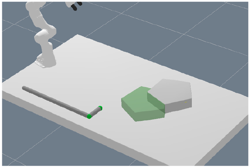
In this experiment, we consider a scenario where objects on a table should be moved to a desired goal configuration (position and orientation on the table) with one robot arm. Compared with the last experiment (Section 5.2), the objects are too large to be grasped. Furthermore, they can be completely out of reach of the robot. Therefore, the robot has to use a hook-shaped tool to push and/or pull the object to the desired location. See Figure 18a or 19 for a typical example scene. The goal pose in these scenes is visualized in transparent green.
Visualization of the action–object image encodings
Example test scene of the pushing experiment containing a triangular prism as the object. The green prism visualizes the target location.
5.3.1. Action operators and optimization objectives
The equations of motion of the object that should be pushed are taken from Toussaint et al. (2020), where it is modeled with quasi-static dynamics based on the Newton–Euler equations in the plane with friction. These equations of motion enter the optimization problem in terms of equality constraints.
We define three action operators,
A
The second action operator
As an important extension to Toussaint et al. (2020), where the PoA is constrained to be anywhere on the surface of
Although the PoA mechanism of Toussaint et al. (2020) can, in principle, figure out from which side to push an object, we found that without introducing
The PoA allows to model both sliding and sticking contacts. However, here we consider the sliding case only, which means that an equality constraint is added that ensures that the tangential component of the force on the surface of
The two different parts
Note that one could also represent those geometric features of the stick in the image space (then the
Finally, the
We consider a maximum of two consecutive pushes. Therefore, in summary, if
5.3.2. Training/test data generation
We sampled 10,000 scenes containing boxes of different sizes, positions, and orientations, as well as 10,000 scenes with triangular prisms, again of different sizes, positions and orientations. Both are combined into one dataset, leading to 20,000 scenes in total, i.e., we train one network on both boxes and triangular prisms. For the boxes, the scene parameter space has dimension eight, and for the triangular prisms, the scene parameter space has dimension seven.
As, for this experiment, the LGP tree is relatively small (but still too large for satisfactory performance at test time), we can actually compute all solutions within reasonable time. Specifically, there are 72 action sequences for each box scene and 42 for each triangular prism scene. Eight of the 72 for the box are action sequences of length 3, and 64 are of length 4. For the triangular prisms, 6 are of length 3, and 36 are of length 4. Therefore, the dataset contains the feasibility of all possible action sequences of each sampled scene.
Representing the pushing actions in the image space allows us to have the same input encoding for both the triangular prisms and the boxes, although they have a different number of faces.
For the test data, we generated 1,000 scenes with the same method, but a different random seed, 500 with boxes and 500 with triangular prisms. For the boxes, 462 scenes contained at least one feasible solution, for the triangular prisms only 369, which then serve as the actual test scenes. In the test dataset, 14.4% of the action sequences for the boxes are feasible, 9% for the triangular prisms. Among those, 5.7% (9%) are of length 3 and 94.3% (91%) are of length 4 for the boxes (triangular prisms).
Note that for every feasible action sequence of length 3, there exists also a feasible one of length 4, namely by pushing two times from the same side. This pushing from the same side twice, however, can also be useful to find a cost-effective (or even feasible) solution, because, owing to the regularization cost term, sliding movements are penalized when the contact between the tool and the object is established. Two consecutive pushes from the same side allow the robot to reposition the contact location without creating large regularization costs.
5.3.3. Performance: results on test scenarios
In Figure 20, we visualize a typical sequence of motions for the pushing scenario.
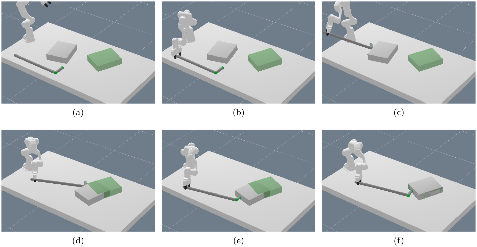
Typical sequence of motions for the pushing experiment: (a) initial scene; (b)
Figure 21 shows the number of NLPs that have to be solved to find a feasible solution with the neural network for the test scenarios. As one can see, for sequence length 3, for both boxes and triangular prisms the network always finds a feasible solution as its first prediction. For sequence length 4, the median of NLPs that have to be solved for boxes is one, for triangular prisms the performance is slightly worse with a median of 2, but still a high performance.
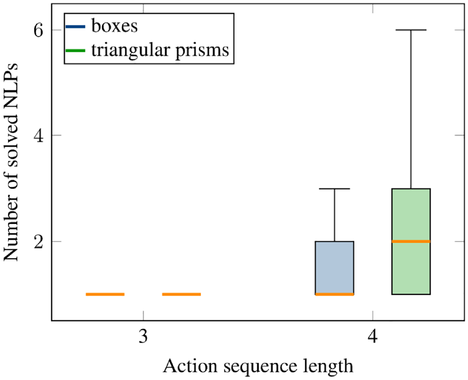
Performance on test scenes for the pushing experiment with our proposed neural network. The network was trained on both boxes and triangular prisms.
The network finds in 30% (23%) of the box (triangular prism) test cases a solution with sequence length 3 and in 70% (77%) of cases a solution with sequence length 4.
For this evaluation, the network has been trained on both boxes and triangular prisms. When we train separate networks for the two different shapes and then evaluate on only those different shapes separately, we do not see a significant difference in the performance.
5.3.4. Comparison with LGP tree search
Compared with kinematic problems as considered in Section 5.2, it is less clear how to define lower bounds that are useful for the pushing scenario that contains dynamic models. Therefore, we compare the performance with LGP tree search without lower bounds, i.e., where directly the full path optimization problem for a chosen action sequence is computed. When we report the number of NLPs that have to be solved to find a feasible solution with LGP in this section, we refer to the expected value when randomly selecting action sequences, which we can determine because, as mentioned in Section 5.3.2, the search tree is small enough for us being able to check the feasibility of all possible action sequences of the test scenes for comparison.
As can be seen in Figure 22, utilizing the network leads for both the triangular prisms and the boxes to a great speedup compared with randomly selecting action sequences. Note that in Figure 22b, LGP has an expected value of exactly 6 for sequence length 3, because for all triangular prisms in the test scenes only a single one of the 6 possible action sequences each was feasible.
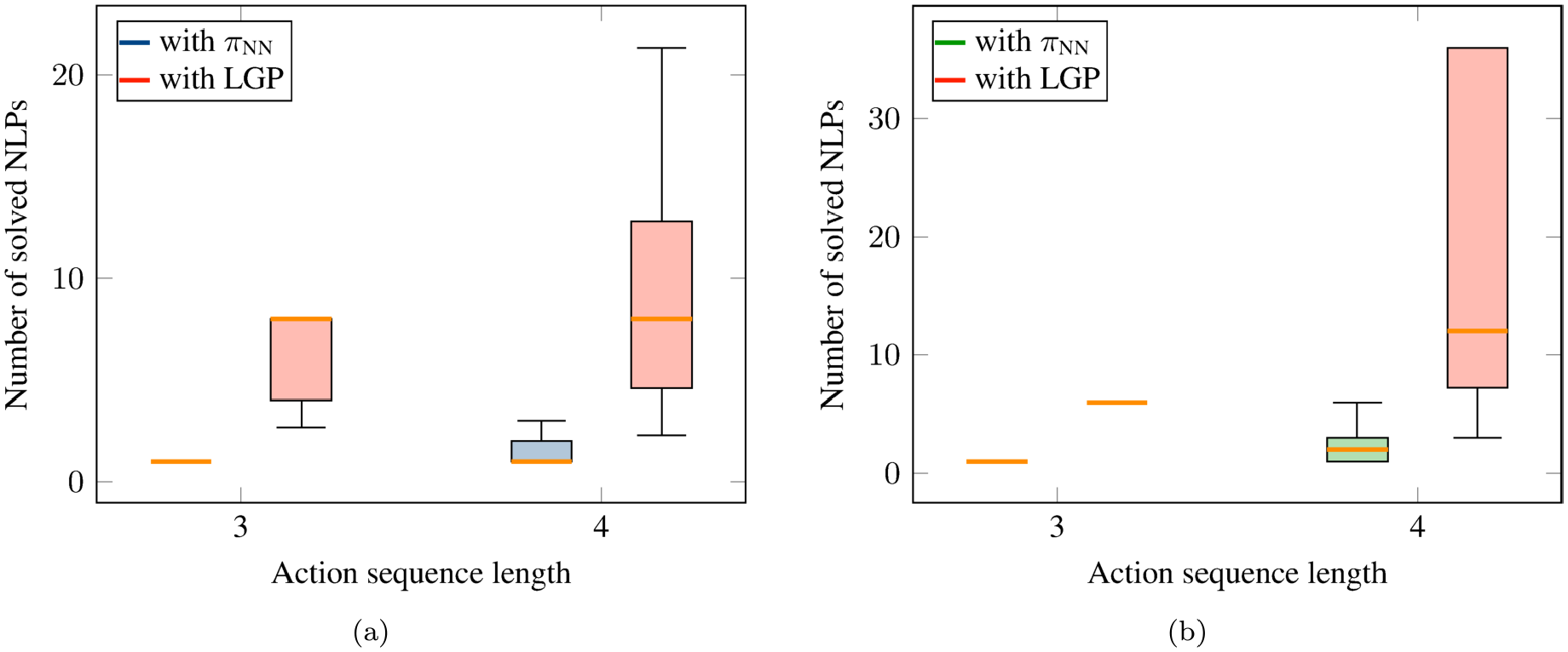
Comparison of LGP with our proposed neural network on test scenes for the pushing experiment: (a) comparison with LGP on box scenes; (b) comparison with LGP on triangular prisms scenes. The network was trained on both boxes and triangular prisms. In (b) the second median line from the left corresponds to LGP.
5.3.5. Generalization to other shapes
The network is trained on box-shaped objects and triangular prisms. Our proposed image based representation for expressing the sides from which the object should be pushed and the desired goal pose allow in principle also other shapes as input to the neural network. Even if there are more push-faces, the algorithm can directly handle this. We therefore tested whether the network can generalize with good performance to other shapes than boxes and triangular prisms, in this case penta prisms.
In order to do so, we generated 200 test scenes that contain penta prisms of different sizes, positions, and orientations as well as different goal poses. See Figure 23 for an example test scene. For penta prisms, there are 110 different action sequences up to length 4 (10 of length 3, 100 of length 4). By solving the NLPs corresponding to all 110 different action sequences, we obtained 188 feasible scenes, which then are the test scenes for this experiment. A total of 13.7% of the action sequences are feasible, among which 3.5% are of length 3 and 96.5% of length 4.
Generalization to other shapes. Example test scene of pushing experiment containing a penta prism. During training the network has only seen boxes and triangular prisms.
Figure 24a reports the number of solved NLPs to find a feasible solution. This figure also contains a comparison with the expected value with LGP. As one can see, the network literally just generalizes to penta prisms, although during training the network only has seen boxes and triangular prisms. The performance is identical to the performance of solving scenes containing boxes (see Figure 21), which is remarkable. For sequence length 3, in all cases the first predicted sequence was feasible, for sequence length 4 the median was 1, the upper whisker 3. Further, in all of the 188 test scenes a solution was found. However, it also has to be noted that the optimizer has full access to the shape of the penta prism. Nevertheless, the network is capable of predicting the push sequence and from which side with high performance for penta prisms, which clearly are not contained in the dataset.
In addition, we tested whether a network that was trained only on boxes, i.e., no triangular prisms, can also generalize to penta prisms. As can be seen in Figure 24b, although the performance is slightly worse for sequence length 4 (median 2 compared with 1 and upper whisker 6 compared with 3), it still generalizes.
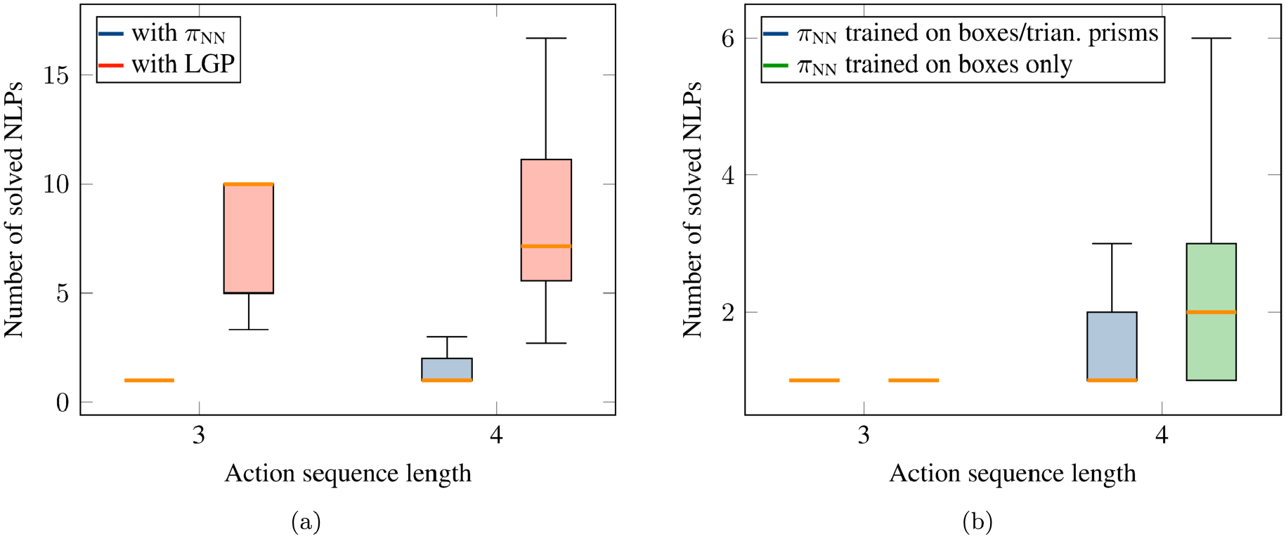
Generalization to penta prism shapes for the pushing experiment. (a) Performance with a network trained on boxes and triangular prisms as well as comparison with LGP without the network. (b) Performance of a network trained on boxes and triangular prisms or boxes only. During training of the network, only boxes and triangular prisms were present in the scene.
5.3.6. Completeness and feasibility threshold
In Table 4 we report the number of test scenes where the network could not find a solution for different feasibility threshold strategies. According to Proposition 1, when using the feasibility threshold together with the discounting adjustment (see Section 4.6.1), prediction errors of the network cannot prevent a feasible solution from being found if it exists. Indeed, as can be seen in the first row of Table 4, in all test scenarios, the adjustment mechanism of the threshold enables the network to not miss a single solution. This holds true for testing on both boxes and triangular prisms as in the training set, but also for penta prisms which shape the network has never seen during training.
Number of test scenes (pushing experiment) for which no solution was found with the network for different feasibility threshold strategies. The first row with
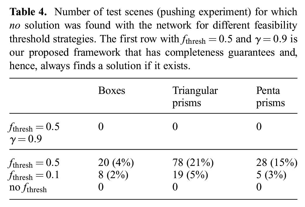
In comparison, if only the feasibility threshold
5.3.7. Cost prediction
In Section 4.8, we proposed how the framework cannot only be used to find feasible solutions, but also to take the trajectory costs into account. This section analyzes both the performance of the cost prediction network to find a feasible solution and determines whether lower cost solutions can be found.
First, the performance in terms of the number of NLPs that have to be solved to find a feasible solution is exactly the same as with the feasibility network (the performance boxplot is identical to Figure 21 and therefore not shown again) and also for every feasible scene a solution was found.
In addition, utilizing the cost prediction network, in 78.6% of the test scenarios with boxes and 88.1% with triangular prisms, the first found solution had a lower cost than with the feasibility prediction network.
For the pick-and-place experiment of Section 5.2, it is intractable to compute all possible action sequences to find the cost optimal one. As, for this scenario, we can actually compute the costs for all sequences, we can investigate how close the first found solution utilizing the cost prediction network is to the real lowest cost over all possible action sequences. Figure 25(a) and (b) show this for the box and triangular prism test scenarios, respectively. These figures report the cost achieved with the network divided by the optimal cost. This means that a value of 1 corresponds to the case where the cost optimal solution was found as the first prediction, a value of 2 corresponds to the case where the found cost was twice as high as the optimum, etc.
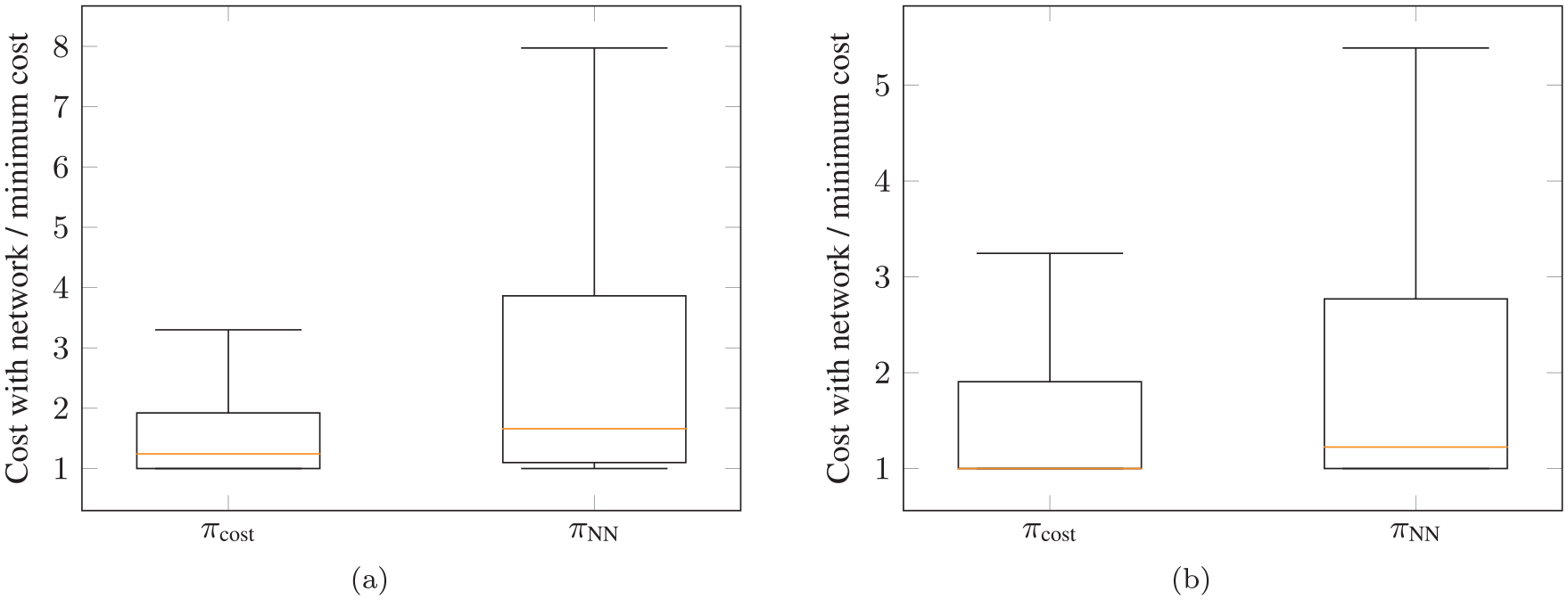
Achieved trajectory costs in comparison with the overall optimum for the first found feasible solution with the cost prediction network
One can clearly see that by utilizing the cost prediction network one can achieve considerably lower costs with the first prediction compared with performing feasibility prediction only. The median for the boxes is very close to 1 and for the triangular prisms the median is 1, i.e., in half of the cases the first found solution was the cost optimal solution.
6. Discussion
Sequential manipulation problems as considered with TAMP approaches are difficult for several reasons. First, the sequential nature not only implies a huge combinatorial complexity of possible high-level action sequences, but also challenging non-convex motion planning problems, where multiple constraints at different phases of the motion have to be coordinated globally (Dantam et al., 2018; Driess et al., 2019a; Garrett et al., 2020; Orthey et al., 2020; Xu et al., 2020). For example, the hook has to be grasped in a certain way in order for it to be possible to push the object to an intermediate position from which the final push to the goal can then be executed.
LGP is one approach to address this by introducing discrete variables that are subject to logic rules to make the trajectory optimization for sequential manipulation problems more tractable, while retaining the property of being able to coordinate the motions in the different phases of the trajectory with global consistency. This, however, implies a combinatorial complexity, significantly increasing the computation time to find a solution, because many, mostly infeasible optimization problems have to be solved.
A key property of TAMP algorithms is that they show remarkable generalization capabilities with respect to different scenes with many and different numbers of objects, changing geometries, etc. This is another reason why sequential manipulation problems are difficult, because the variety of tasks in different scenes demands strongly generalizing algorithms. From a learning point of view, it is challenging to create datasets that cover such a variety of scene parameters and goals.
We make essential contributions in several of those regards. First, we address the combinatorial complexity that is introduced through the discrete variables by learning a goal conditioned network that guides the search over the discrete variables in a way that most of the time the search is eliminated, leading to large speedups in solution times. Further, we demonstrated our method not only on a single problem instance, but on a variety of scenes, including different object parameters, goals, but especially increasing numbers of objects, although only a fixed number of objects was present in the training set. Moreover, our proposed image representation enables generalization to different shapes of objects than those present in the training data.
The generalization to more objects than during training is a major advantage of the image-based encoding of the scene we proposed compared with a fixed feature representation. As shown in Section 5.2.9, the network is able to maintain high performance if more objects are added to the scene. However, one also has to state that this kind of generalization to multiple objects has to be understood in the sense that the network correctly chooses up to two objects which have to be manipulated (multiple times) to solve the task. The network realizes a kind of attention mechanism, operating on only the relevant parts of the environment. This could also be observed in the generalization experiment to cylinders (Section 5.2.11), where the network does not attempt to grasp cylinders which are too large, although it has never seen cylinder-shaped objects during training. Being able to identify which objects are relevant to solve the task is crucially important and the reason for why the network can find solutions quickly even in scenarios where there are nearly half a million candidate action sequences, cf. Table 1 and Figure 13. We believe that such an attention mechanism is the key to tackling even more realistic environments with far greater combinatorial complexities such as household scenarios.
Although we do not expect the network to generalize with high accuracy to scenarios where more than two objects have to be manipulated in order to solve the task without a broader training distribution, we have investigated in Section 5.2.10 and Table 3 that for scenes where three objects have to be manipulated with action sequence length up to eight (training distribution has a maximum sequence length of six and contains only two objects), the network still leads to a speedup in finding a solution up to several orders of magnitude compared with LGP without the network. However, in this case, the network acts as a heuristic that does not eliminate search, since more optimization problems had to be solved to find a feasible solution compared with the scenarios where only two objects in the scene have to be manipulated.
Our approach assumes that we are able to extract segmentation masks of each object from the raw image of the initial scene. Many methods such as Mask R-CNN (He et al., 2017) have been developed for object segmentation. Although definitively challenging, we believe that the ability to segment objects in an image is a necessary condition for many robot applications that rely on perception in uncontrolled environments and, hence, a reasonable assumption to make. In particular, without being able to detect objects, defining the TAMP problem in the first place is unclear. There are also recent approaches that estimate the state of the symbolic domain from image segmentations (Kase et al., 2020; Mukherjee et al., 2020; Zhu et al., 2020).
As already mentioned in Section 5.2.12, although the generation of the discrete action sequences only relies on images and these object segmentations, the trajectory optimization still requires object models in terms of their shapes and poses. Hence, a perception pipeline is required to extract these properties from the raw image observations. Future work could investigate how to make the motion generation given a discrete action sequence less reliant on exact object models (Driess et al., 2021a,b; Manuelli et al., 2019; Qin et al., 2019; Simeonov et al., 2020; Suh and Tedrake, 2020; Wang et al., 2020).
Despite this, we have shown that the image representation has advantages (generalization to multiple objects/shapes, encoding geometry information) independently from whether object models are known or not. This means that one way to interpret the images in this work is not solving manipulation from raw perception, but a flexible state/action representation for long-horizon reasoning. Still, we believe that this representation is also one step to connect TAMP more closely to real perception.
One of the main limitations of this work, in our opinion, is that the initial scene image has to contain all information that is necessary to reason about the action sequence.
Therefore, we have focused on tabletop manipulation scenarios, because, in this case, the assumption that the image contains sufficient information about the scene/task is reasonable for the considered tasks. Total occlusions, for example, if an object is inside a cabinet, cannot be handled with the current approach. Partial occlusions, as long as the image still contains sufficient information, can in principle work. In a scenario where objects are stacked on top of each other in the initial scene, the top-down camera view as considered here is insufficient, but could be replaced with an angled view. As long as object masks and the image are provided in such a way that still the relevant object geometries can be inferred, we expect the method to work just as well. In mobile manipulation setups, the proposed methodology would not be applicable for solving the whole problem, because it is unrealistic to assume that a single image contains all necessary information. However, we believe that the ideas of this work could also be useful for solving parts of the manipulation problem (subgoals) quickly and repeatedly in an online setup. Most existing TAMP approaches assume full knowledge about the initial state, even in mobile manipulation settings. Only recent work starts to address these issues by belief-space planning in the context of TAMP (Garrett et al., 2019; Phiquepal and Toussaint, 2019).
In general, a major strength of the LGP formulation is that the actions imply constraints that only partially determine the behavior of the trajectory. The overall trajectory is then optimized with global consistency, filling in the remaining degrees of freedoms, or action parameters as they are called in other TAMP approaches. This property of LGP allows us, for example, to efficiently generate handover motions or removing of obstacles without explicitly needing to enumerate handover poses or the placement positions of the occupying obstacle. However, scaling to significantly longer action sequence lengths, it becomes clear that it is neither necessary nor feasible to optimize trajectories with complete global consistency. Introducing further hierarchies (Kaelbling and Lozano-Pérez, 2011) or breaking the manipulation down into (less-dependent) subgoals (Driess et al., 2019a; Hartmann et al., 2020, 2021) becomes necessary.
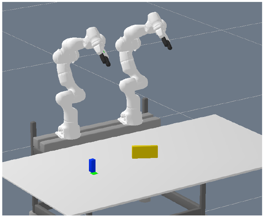
Goal region (green) is only partially occluded by the blue object, such that the yellow object can be placed on the goal without removing the blue object first. The network find this as its first proposed solution.
Instead of a black-box reward function, we specify the manipulation planning goal in terms of object masks similar to the action–object images. This goal–object image contains both the mask of the target object and the goal, as well as a channel of the whole scene. Therefore, the goal specification can encode the target object, the goal and other objects in the scene in such a way to take their geometric relations into account. Figure 26 shows a scenario where the goal is only partially occluded by the blue object. In this case, the network is able to realize that the yellow object can be placed on the green goal region without removing the blue object first and proposes this as the first solution. For a stacking scenario, one could think of having multiple object masks as part of the goal specification to encode which objects should be stacked. However, such goal specifications assume that masks of the unobstructed goal region for the pick-and-place experiment and the mask of the desired target pose for the pushing experiment can be generated. Investigating other goal specifications is an important topic for future research.
To show the completeness of our framework (proposition 1), we assumed (assumption 1) that the nonlinear trajectory optimizer numerically converges to a feasible solution if the problem is indeed theoretically feasible. Although such assumptions usually only hold for convex problems and our trajectory optimization problems are, even for a fixed action sequence, non-convex, we empirically found that the optimizer converges reliably. The introduction of the additional discrete decisions for the pushing scenario was important for this robustness.
We considered boxes, cylinders, triangular, and penta prisms, all of different sizes, in this work. Although we argue that an advantage of the input images is their principal capability of representing and generalizing to different shapes, we assumed that the underlying trajectory optimization method can handle those shapes. In order to achieve this, the paradigm of this work is to introduce a set of discrete decisions for each subtask (grasping, pushing, and placing). These decisions can (not strictly) be understood as a means to enumerate local optima such that, given the discrete decisions, the optimizer is then able to find the remaining degrees of freedom for global consistency robustly. In the case of grasping, those decisions enumerate graspings from different sides of the object. For pushing, they specify the side from which the object should be pushed. In principle, one could think of introducing more such discrete decisions to deal with a greater variety of shapes. However, generalizing this idea to arbitrary shapes is not directly straightforward for multiple reasons. On the one hand, it becomes less clear how to define constraints realizing the subtasks for arbitrary shapes in a way that, in the paradigm of this work, benefits from parameterizing them with discrete decisions to make trajectory optimization with those constraints tractable. On the other hand, if too many discrete decisions are introduced, then the branching factor of the LGP tree increases significantly. This might not only lead to a harder learning problem, but it also becomes more challenging to generate data containing enough feasible action sequences in a reasonable amount of computation time. As illustrated in Figure 6, we considered four different graspings from above the object. In our previous work (Driess et al., 2020b), we have shown for a single action that the feasibility of not only top, but additionally also side grasps can be predicted from a similar input representation as in the present work. We anticipate that our network would, in principle, be able to take side grasps into account as well. In order to address the data generation problem in this case due to an increased branching factor, bootstrapping the learned network for data generation would be one way. We believe that integrating grasping of complex objects within long-horizon tasks where the way an early grasp is executed has to be coupled with later phases of the motion is an important future research topic.
7. Conclusion
In this work, we have proposed a neural network that learns to predict promising discrete action sequences for sequential manipulation problems from an initial scene image and the task goal as input. In most cases, the first sequence generated by the network was feasible. Hence, despite the fact that the network can act as a search heuristic, there was very little search over the discrete decisions required and, consequently, often only one trajectory optimization problem had to be solved to find a solution to the TAMP problem.
Although being trained on only two objects present at a time, the learned representation of the network was able to be generalized to scenes with multiple objects and other shapes while still showing a high performance.
We have shown that the approach can be applied not only to kinematic pick-and-place problems as is typical in TAMP, but also to a scenario where an object has to be pushed with a tool to a desired target location. Here one can see another advantage of the image representation, because the network generalized to other shapes than during training.
A main assumption and, therefore, main limitation of the proposed method is that the initial scene image has to contain sufficient information to solve the task, which means that there should be no total occlusions or other ambiguities.
Footnotes
Appendix. Index to multimedia extensions
Archives of IJRR multimedia extensions published prior to 2014 can be found at http://www.ijrr.org, after 2014 all videos are available on the IJRR YouTube channel at http://www.youtube.com/user/ijrrmultimedia
Demonstration of the planned motions both in simulation and with a real robot
Acknowledgements
We thank the anonymous reviewers for their helpful comments.
Funding
The author(s) disclosed receipt of the following financial support for the research, authorship and/or publication of this article: Danny Driess thanks the International Max-Planck Research School for Intelligent Systems (IMPRS-IS) for support. Marc Toussaint is grateful for the Max-Planck Fellowship at the Max-Planck Institute for Intelligent Systems in Stuttgart. This research has been supported by the German Research Foundation (DFG) under Germany’s Excellence Strategy (grant number EXC 2002/1–390523135 “Science of Intelligence”).