
Abstract
Traditional approaches to outdoor vehicle localization assume a reliable, prior map is available, typically built using the same sensor suite as the on-board sensors used during localization. This work makes a different assumption. It assumes that an overhead image of the workspace is available and utilizes that as a map for use for range-based sensor localization by a vehicle. Here, range-based sensors are radars and lidars. Our motivation is simple, off-the-shelf, publicly available overhead imagery such as Google satellite images can be a ubiquitous, cheap, and powerful tool for vehicle localization when a usable prior sensor map is unavailable, inconvenient, or expensive. The challenge to be addressed is that overhead images are clearly not directly comparable to data from ground range sensors because of their starkly different modalities. We present a learned metric localization method that not only handles the modality difference, but is also cheap to train, learning in a self-supervised fashion without requiring metrically accurate ground truth. By evaluating across multiple real-world datasets, we demonstrate the robustness and versatility of our method for various sensor configurations in cross-modality localization, achieving localization errors on-par with a prior supervised approach while requiring no pixel-wise aligned ground truth for supervision at training. We pay particular attention to the use of millimeter-wave radar, which, owing to its complex interaction with the scene and its immunity to weather and lighting conditions, makes for a compelling and valuable use case.
1. Introduction
The ability to localize relative to an operating environment is central to robot autonomy. Localization using range sensors, such as lidars (Levinson and Thrun, 2010; Wolcott and Eustice, 2015) and, more recently, scanning millimeter-wave radars (De Martini et al., 2020; Park et al., 2019; Saftescu et al., 2020), is an established proposition. Both are immune to changing lighting conditions and directly measure scale, while the latter adds resilience to weather conditions.
Current approaches to robot localization typically rely on a prior map built using a sensor configuration that will also be equipped on-board, for example a laser map for laser-based localization. This article looks at an alternative method. Public overhead imagery such as satellite images can be a reliable map source, as they are readily available, and often capture information also observable, albeit perhaps in some complex or incomplete way, by sensors on the ground. We can pose the localization problem in a natural way: finding the pixel location of a sensor in an overhead (satellite) image given range data taken from the ground. The task is, however, non-trivial because of the drastic modality difference between satellite images and sparse, ground-based radar or lidar.
Recent work on learning to localize a ground scanning radar against satellite images by Tang et al. (2020b) provides a promising direction which addresses the modality difference by first generating a synthetic radar image from a satellite image. The synthetic image can then be “compared” against live radar data, expressed as 2D images from a “bird’s eye” perspective, for pose estimation. Such an approach learns metric, cross-modality localization in an end-to-end fashion, and therefore does not require hand-crafted features limited to a specific environment.
The method in Tang et al. (2020b) trains a multi-stage network, and needs pixel-wise aligned radar and satellite image pairs for supervision at all stages. This, in turn, relies on sub-meter and sub-degree accurate ground-truth position and heading signals, which in practice requires high-end GPS/inertial navigation system (INS) and possibly bundle adjustment along with other on-board sensor solutions, bringing in burdens in terms of cost and time consumption.
To address this issue, building on the work of Tang et al. (2020b), we propose a method for localizing against satellite imagery that is learned in a self-supervised fashion. The core idea is still to generate a synthetic image with the appearance and observed scenes of a live range sensor image, but pixel-wise aligned with the satellite image. Yet, we relax the requirement on pixel-wise aligned data pairs and assume only a coarse initial pose estimate is available from a place recognition system, such that there is reasonable overlap between the live ground sensor field of view and a queried satellite image. Our method does not solve the global localization problem. Instead, given a coarse initial pose estimate from place recognition, our method solves the metric localization of a range sensor using overhead imagery, providing a refined
Vitally, here we make no use of metrically accurate ground truth for training. Note also that although designed for localizing against satellite imagery, our method can naturally handle other forms of cross-modality registration, such as localizing a radar against a prior lidar map. Figure 1 shows synthetic images generated by our method used for pose estimation.
Given a map image of modality
To the best of the authors’ knowledge, our proposed method is the first to learn the cross-modality, metric localization of a range sensor in a self-supervised fashion. Our method is validated experimentally on multiple datasets and achieves performances on-par with a state-of-the-art, supervised approach. Even though our method does not solve the global localization problem and instead relies on an external place recognition system, it can nevertheless be utilized to greatly refine the sensor’s metric pose starting from a coarse initial pose estimate, all in the absence of any prior sensor maps.
This article is an extended version of our prior work (Tang et al., 2020a). The improvements include a more detailed explanation for the motivation of our method to tackle the problem of localizing range sensors using satellite imagery (Section 3) and a more thorough description of our method (Section 4). For experimental validation (Section 6), we present additional qualitative results, an ablation study with reduced training data, a study on the trade-offs between network width and depth and solution quality, and an analysis on the choice of image resolution. We also introduce an introspective strategy at inference time to handle initial pose offsets larger than in the training data. Finally, we show with unsupervised domain adaptation, models trained using radar data can be utilized for localization between lidar and overhead imagery, and vice versa.
2. Related work
Our approach is related not only to other works in the field of localization using overhead imagery and the general theme of cross-modality localization, but also to learned methods for range sensor state estimation and unsupervised image generation. We provide a broad coverage of the most relevant research in these subjects in this section.
2.1. Localization using overhead images
Localization using aerial or overhead images has been of interest for the community for over a decade. The methods in Leung et al. (2008), Li et al. (2014), and Parsley and Julier (2010) localize a ground camera using aerial images, by detecting Canny edges from aerial imagery, and matching against lines detected by a ground camera. Several other vision-based approaches project the ground camera images to a top-down perspective via a homography, and compare against the aerial imagery by detecting lane markings (Pink, 2008), Speeded Up Robust Features (SURF) (Noda et al., 2010), or dense matching (Senlet and Elgammal, 2011). Recent work by Chebrolu et al. (2019) localizes a ground robot in a crop field by matching camera features against landmarks from an aerial map, and explicitly incorporates semantics of crops to reduce ambiguity.
Metric localization of range sensors or point-clouds against overhead imagery requires further pre-processing owing to the modality difference. Kaminsky et al. (2009) projected point-clouds into images and matched against binary edge images from overhead imagery. The method of Kaminsky et al. (2009) also constructs a ray image by ray-tracing each point, and introduces a free-space cost to aid the image registration. The work by de Paula Veronese et al. (2015) accumulates several lidar scans to produce dense lidar intensity images, which are then matched against satellite images utilizing normalized mutual information. Similar to Kaminsky et al. (2009), several other methods also pre-process the aerial image before matching against ground laser observations, for example using edge detection (Kümmerle et al., 2011) or semantic segmentation (Dogruer et al., 2010). In contrast to these approaches, our method directly learns the metric localization of a range sensor end-to-end, without the need for careful pre-processing or manual feature definition.
Closely related to our method is the seminal work on learning to localize a ground radar against satellite imagery by Tang et al. (2020b). As discussed previously, the method in Tang et al. (2020b) requires pixel-wise aligned ground truth for supervision, whereas our method is self-supervised.
2.2. Cross-modality localization
Other forms of cross-modality localization have also been heavily studied by the community. Several works propose to localize a forward-facing camera against a prior 3D point-cloud map (Caselitz et al., 2016;Wolcott and Eustice, 2014; Xu et al., 2017). Carle and Barfoot (2010) localized a ground laser scanner against an orbital elevation map. The works in Wang et al. (2019), Boniardi et al. (2017), Wang et al. (2017), and Mielle et al. (2019) localize an indoor lidar or stereo camera against architectural floor plans. Recently, Yin et al. (2021) proposed a joint learning system for radar place recognition using a prior lidar database, and achieves state-of-the-art results on the Oxford Radar RobotCar Dataset (Barnes et al., 2020) and MulRan Dataset (Kim et al., 2020).
OpenStreetMap is a particularly useful publicly available resource for robot localization. Brubaker et al. (2013) and Floros et al. (2013) concurrently proposed matching visual odometry paths to road layouts from OpenStreetMap for localization. Ruchti et al. (2015) proposed a road classification scheme to localize a ground lidar using OpenStreetMap. Yan et al. (2019) utilized networks pre-trained for point-cloud semantic segmentation, and built a light-weight descriptor to recognize intersections and gaps, and compared against the descriptors of the operating environment built using OpenStreetMap.
2.3. Learning-based state estimation for range sensors
A number of recent works were proposed for learning the odometry or localization of lidars. Barsan et al. (2018) represented lidar data as intensity images, and learned a deep embedding specifically for metric localization that can be used for direct comparison of live lidar data against a previously-built lidar map. Other methods such as Cho et al. (2019); Li et al. (2019), instead, learn deep lidar odometry by projecting lidar point-clouds into other representations before passing through the network. Lu et al. (2019b) learned descriptors from input point-clouds, and utilized 3D CNNs for solving
As an emerging sensor for outdoor state estimation, learning-based methods were proposed for scanning frequency-modulated continuous-wave (FMCW) radars. Aldera et al. (2019) utilized an encoder–decoder on polar image representation of radar scans to reject superfluous points for decreasing computation time in the classical radar odometry method described by Cen and Newman (2019). Barnes et al. (2019) learned image-based radar odometry by masking out regions distracting for pose estimation. Barnes and Posner (2020) learned point-based radar odometry by detecting key points from radar images. Saftescu et al. (2020) encoded images of polar radar scans through a rotation-invariant architecture to perform topological localization (place recognition), which can then be used for querying a previously built map (De Martini et al., 2020). These methods, however, are designed to compare data of the same sensor type, and do not address modality difference. Our approach is similar to Barsan et al. (2018), Cho et al. (2019), Aldera et al. (2019), Barnes et al. (2019), Weston et al. (2019), Saftescu et al. (2020), Barnes and Posner (2020), and Broome et al. (2020) in that we also represent range sensor data as 2D images.
2.4. Unsupervised image generation
A fundamental step in our approach is the generation of a synthetic image before pose computation, where there is no pixel-wise aligned target image for supervision. CycleGAN (Zhu et al., 2017) achieves unsupervised image-to-image transfer between two domains
Several prior works are also geometry-aware. The methods by Shu et al. (2018), Wu et al. (2019), and Xing et al. (2019) use separate encoders and/or decoders to disentangle geometry and appearance. The results are networks that can separately interpolate the geometry and appearance of the output images. Similarly, our method separately encodes information about the appearance and the relative pose offset, resulting in an architecture where the two are explicitly disentangled.
3. Overview and motivation
We seek to solve for the
Previously, Radar–Satellite Localization Network (RSL-Net) (Tang et al., 2020b) was proposed to solve for the metric localization between matched pairs of radar and satellite images. In particular, it aims to generate a synthetic image that preserves the appearance and observed scenes of the live radar image, and is pixel-wise aligned with the paired satellite image. The synthetic image and the live radar image are then projected onto deep embeddings, where their pose offset is found by maximizing a correlation surface. We follow the same general approach, but, unlike RSL-Net, our method learns in a self-supervised fashion.
3.1. Hand-crafting features versus learning
Some of the works listed in Sections 2.1 and 2.2 can achieve decent accuracy on localizing a ground range sensor against aerial imagery. However, they typically rely on pre-processing the aerial images using hand-crafted features or transformations designed for a specific set-up and may not generalize to other sensors or different environments. For example, Kümmerle et al. (2011) focus on detecting edges from a campus dominated by buildings. de Paula Veronese et al. (2015) directly match accumulated lidar intensity images against aerial imagery without pre-processing, yet this is inappropriate for radars due to the complexity of their return signals.
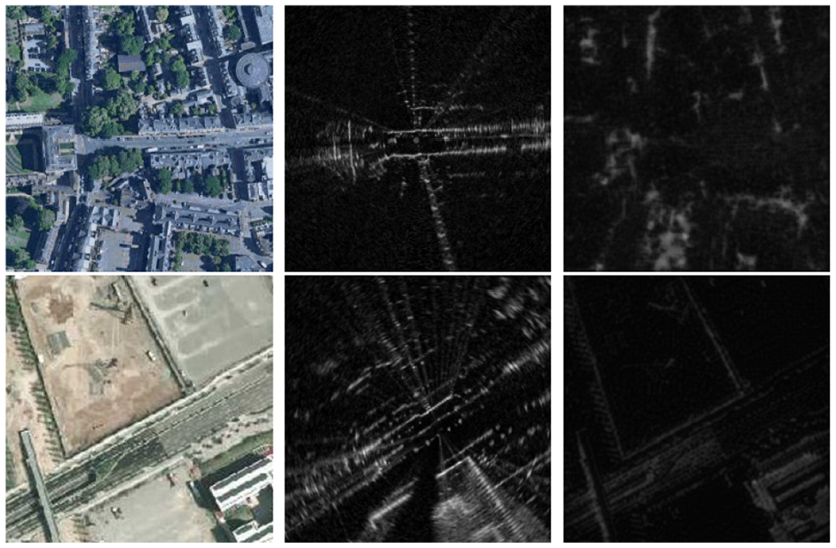
Our data-driven approach instead learns to directly infer the geometric relationship across modalities, remaining free of hand-crafted features. We show in Section 6 the robustness of our method when localizing against satellite imagery in various types of scenes, including urban, residential, campus, and highway (Figure 2).
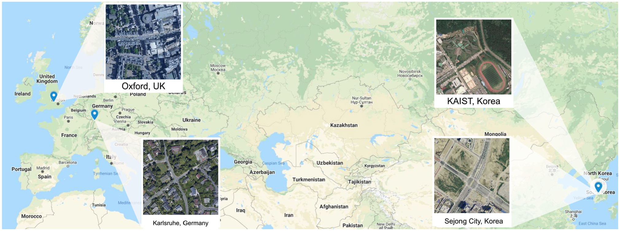
Our method is demonstrated on datasets collected around different locations, at various types of settings including urban (Oxford, UK), residential (Karlsruhe, Germany), campus (KAIST, Korea), and highway (Sejong City, Korea).
3.2. Generating images versus direct regression
A naive approach would be to take a satellite image and a live data image as inputs, and directly regress the pose. Yet, as shown in Tang et al. (2020b), this led to poor results even for the supervised case. Our hypothesis is that when the two images are starkly different in appearance and observed scenes, the problem becomes too complex for direct regression to succeed given current techniques.
Generating synthetic images prior to pose estimation brings two advantages over directly regressing the pose. First, it is a simpler and less ill-posed problem than directly regressing the pose, particularly because we can utilize the live data image to condition the generation. Second, the image generation loss is distributed over an entire image of
3.3. Conditional image generation
We tackle the synthesis of an image of the live data modality
In practice, the map (e.g., satellite) image is a denser representation of the environment than a frame of data captured by a range sensor. Only a fraction of the scenes captured in a satellite map is present in a ground sensor field of view, resulting in the scan to appear drastically different depending on the sensor pose. In other words, the mapping from a satellite image to a range sensor image is not one-to-one, but one-to-many, as illustrated in Figure 3. Figure 4 demonstrates this concept on real data: the overlapping regions of the two satellite images are identical, whereas the two radar images observe different portions of the scene and as such appear drastically different.
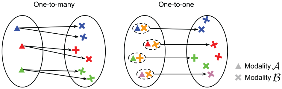
A one-to-many mapping (left) versus a one-to-one mapping (right). Left: the mapping from modality
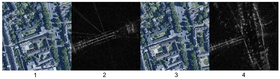
Two radar images captured 15 seconds apart from each other (2 and 4), pixel-wise aligned with satellite images (1 and 3). Though the overlapping scenes in the satellite images are identical, the radar scans appear significantly different, as they capture different regions in their field of view.
By using a naive image-to-image transfer approach, there is no guarantee for the generated image to contain regions of the scene that are useful for pose comparison against the live data image. Figure 5 shows examples of images generated using CycleGAN (Zhu et al., 2017), where the synthetic image highlights different scenes than what are observed by the live data image. The issue with observability or occlusion can potentially be handled by ray-tracing, such as in Kaminsky et al. (2009). However, not only is this computationally expensive, it does not apply to FMCW radars which have multiple range returns per azimuth (see Barnes et al. (2020) and Cen and Newman (2019) for more details on the sensing characteristics of FMCW radars).
Results of CycleGAN: satellite image (left), live radar image pixel-wise aligned with the satellite image (middle), synthetic radar image (right). There is no explicit constraint on which regions of the input satellite image will appear in the output synthetic image. As a result, this leads to large localization error as the synthetic image does not contain scenes observed by the live radar image.
Our approach inherently addresses this problem: by conditioning the image generation with the live data image, we can encourage the synthetic image to capture regions of the scene also observed by the live data image, as shown in Sections 4 and 6. This concept is analogous to learning the mapping on the right of Figure 3, where, by using a pair of satellite and range sensor images as input, the regions of the scene to be present in the output synthetic image is no longer ambiguous, but constrained by the input range sensor image.
4. Self-supervised cross-modality localization
Our localization pipeline is composed of three steps: rotation inference, image generation, and pose estimation. We discuss them in detail in this section.
4.1. Rotation inference
Given a paired map (e.g., satellite) image
Let the

where
However, as originally noted by Tang et al. (2020b), the mapping in (1) is difficult to learn as the inputs
The method in Tang et al. (2020b) proposes to infer the rotation prior to image generation, namely, reducing (1) to two steps:


Here
In Tang et al. (2020b), the rotation inference function
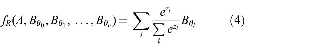
where each
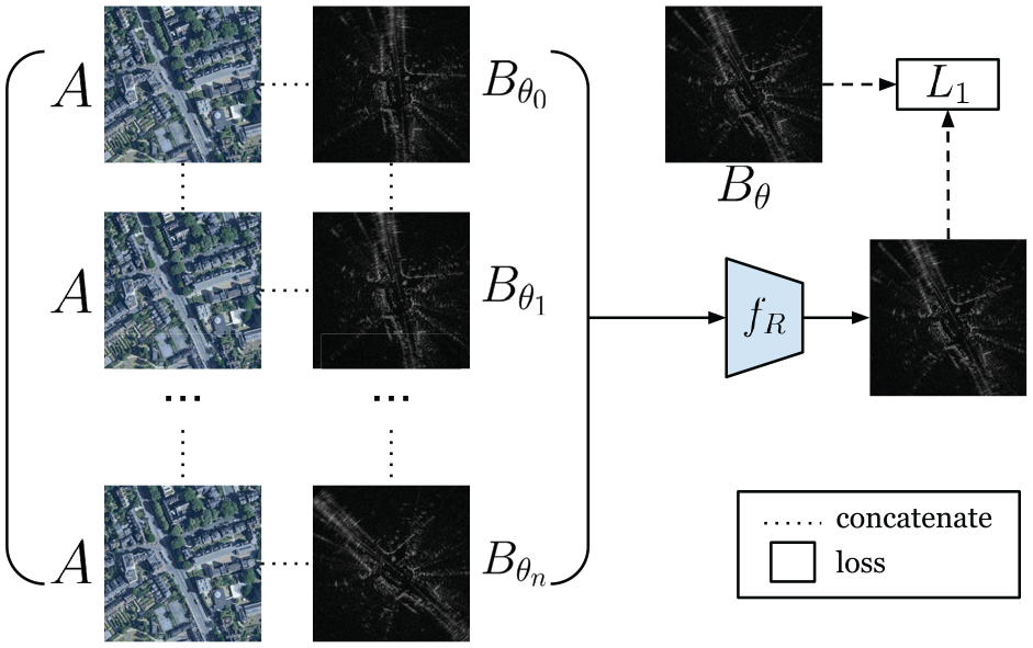
Prior work in Tang et al. (2020b) proposes a network to infer the rotation offset. The rotation offset is found by softmaxing a stack of rotated radar images to produce a radar image with the same heading as the satellite image.
A loss function enforces the output to correspond to
If a metrically accurate heading ground truth
For this reason, while following the same architecture as Tang et al. (2020b), our method for inferring rotation uses a different training strategy that enables self-supervised learning. In order for the network
As such, to learn rotation inference self-supervised, we need to pass through the network
The network is supervised with an


where
Given
The estimate for the rotation offset,
4.2. Image Generation
Given
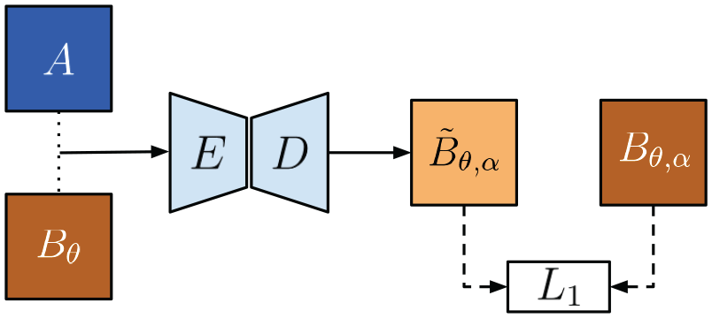
Architecture for image generation in prior supervised approach (Tang et al., 2020b).
In the supervised approach in Tang et al. (2020b), a loss can be formed between the synthetic image and the target:

where
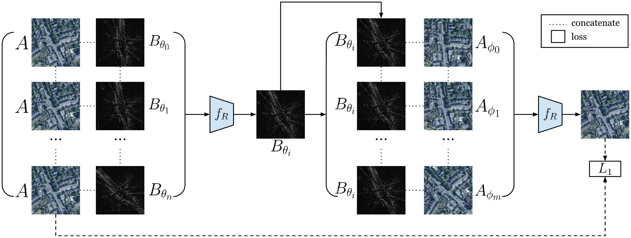
To generate synthetic images self-supervised, we propose an architecture we call PASED, shown in Figure 9. PASED is trained in two steps: the first is a pre-training, intra-modality process that can be supervised with ground truth image targets (top half of Figure 9), whereas the second handles cross-modality comparison (bottom half of Figure 9).
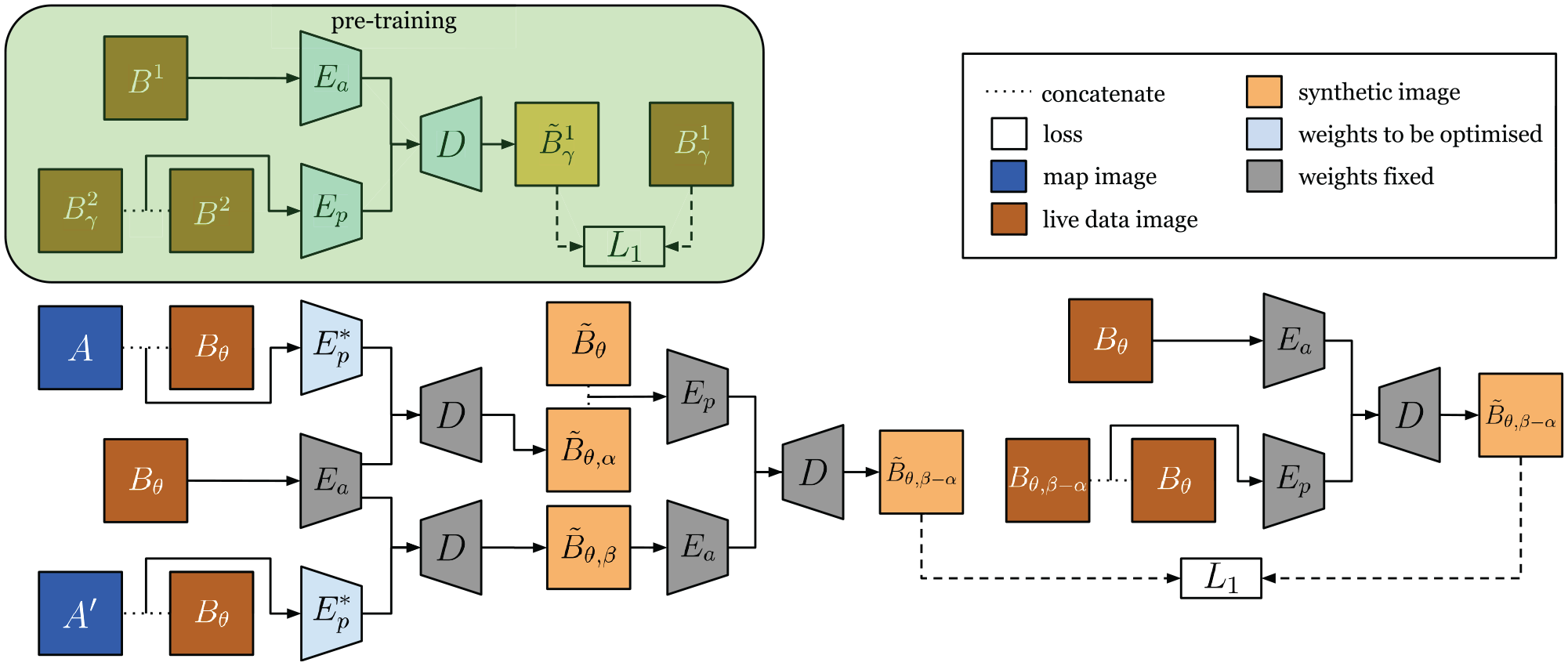
Top: During pre-training, we can learn an appearance encoder
4.2.1. Pre-training step
Taking two random images
In other words, PASED discovers the translation offset between the two images passed as input to
and the parameters for networks
The fact that we use different images
4.2.2. Cross-modality step
In the second step, we fix the weights of
We can apply a known shift to the center position of
Furthermore, given

If we pass

Here
We can shift

We can form
By back-propagation, the loss in (15) optimizes the network
For the loss in (15) to be minimized, two conditions must hold true. First,
4.3. Pose estimation
Taking the pose-aligned synthetic image
The correlation maximization is a parameter-free process that requires no additional learned modules, but is differentiable allowing gradients induced by the downstream loss to propagate to upstream learned modules. In this step, we can infer
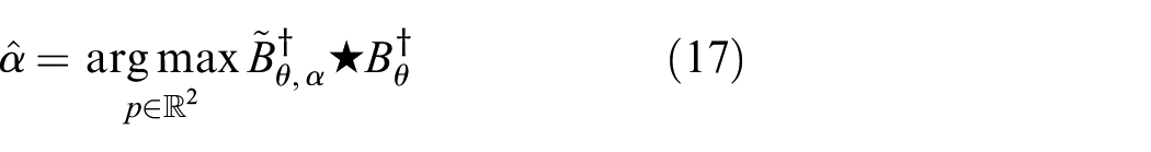
where
The embeddings are thus learned to further ensure the synthetic image and the live image can be correlated correctly. Without ground truth
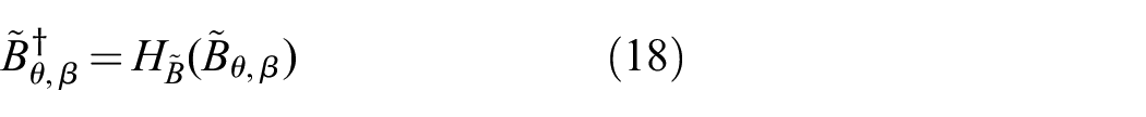
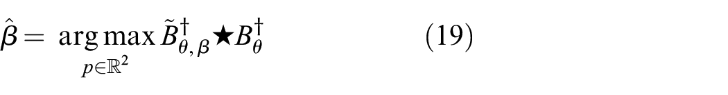
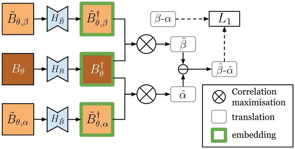
The networks
The difference of the two offsets
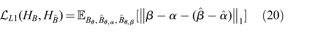
The overall pipeline for data flow at inference time is shown in Figure 11.
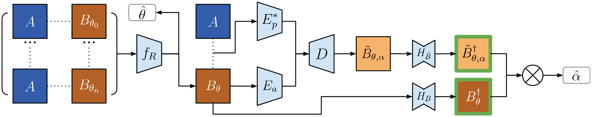
Overall data flow of our method at inference: given map image
5. Implementation details
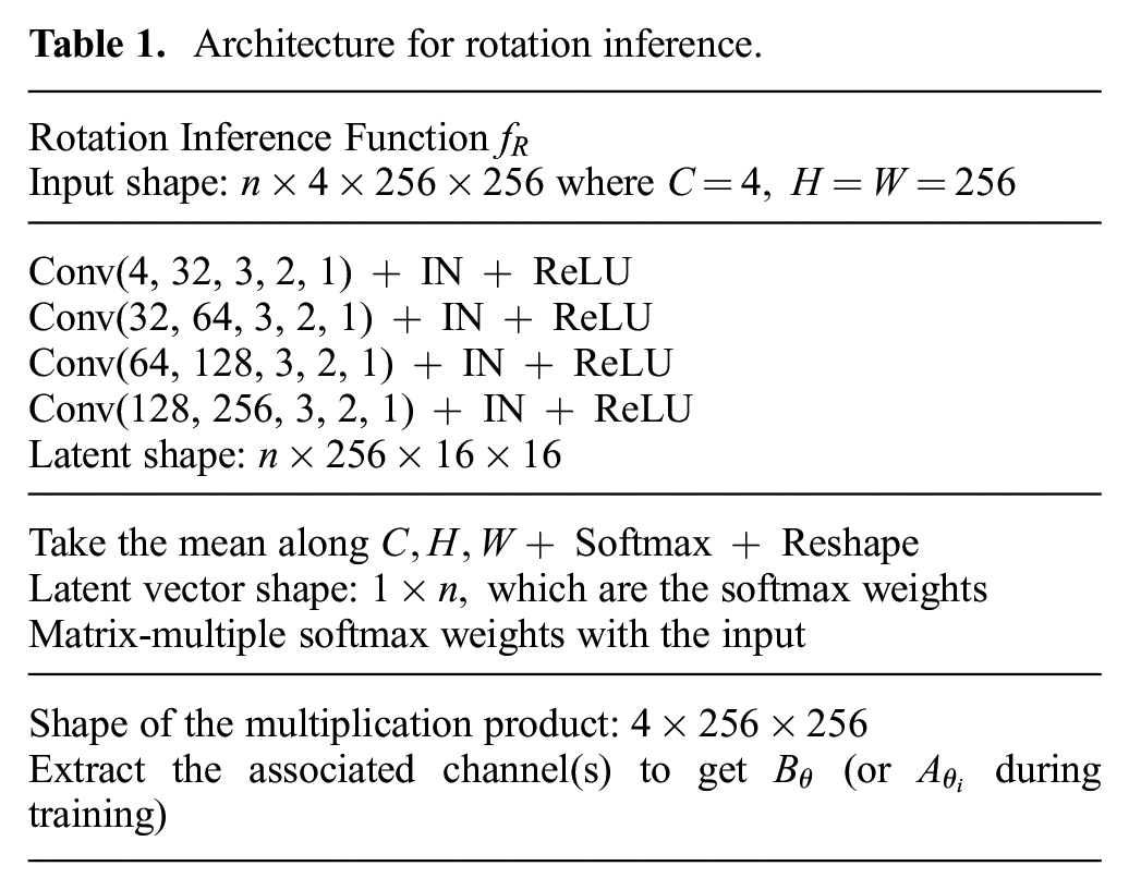
Here we provide details on the architecture of the various networks used in our method, and the associated hyper-parameters. We make use of the following abbreviations.
RP(
Conv(
IN: instance normalization.
ReLU: rectified linear unit.
LReLU(
Drop(
ConvT(
The network architectures are listed in Tables 1 to 4. For comparison against the prior supervised approach, we use the same architectures where possible. We implemented the image generation network for the prior supervised approach to have the same latent space size at the bottleneck, and the same number of down-sample and up-sample layers as in our method.
Architecture for rotation inference.
Architecture of for image generation.
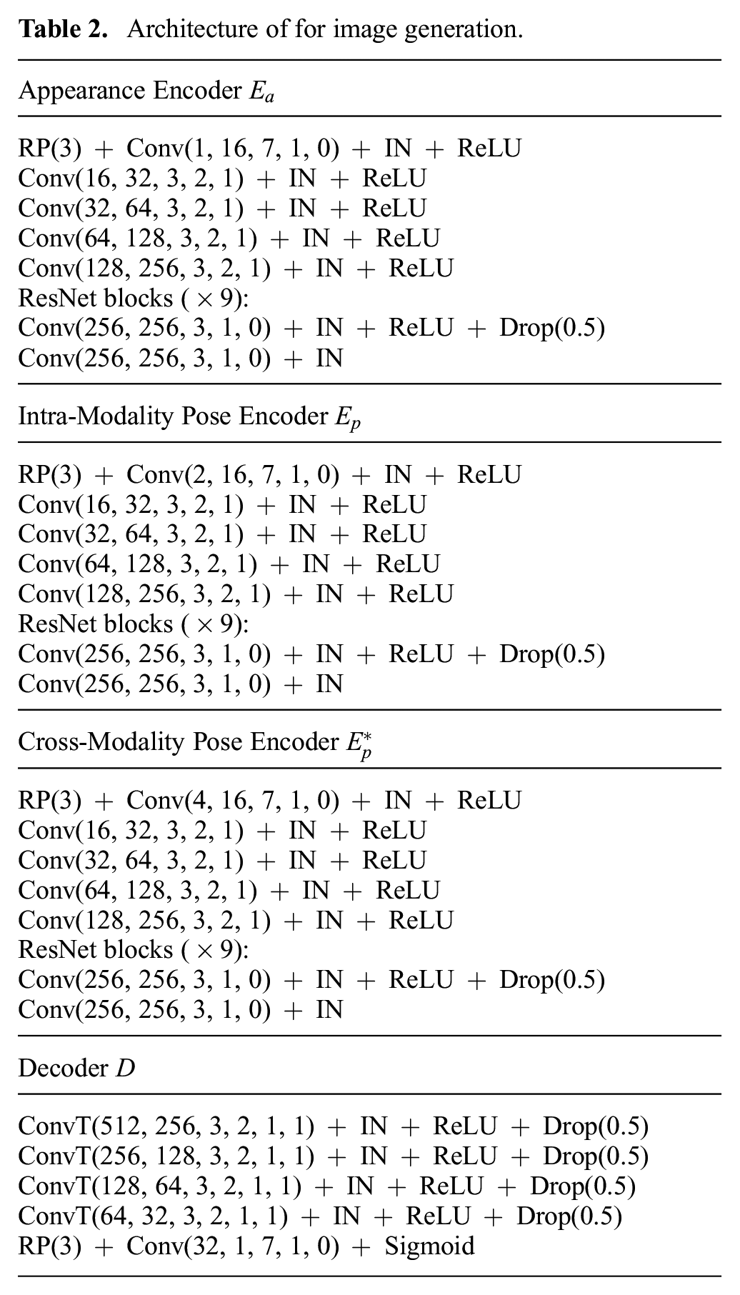
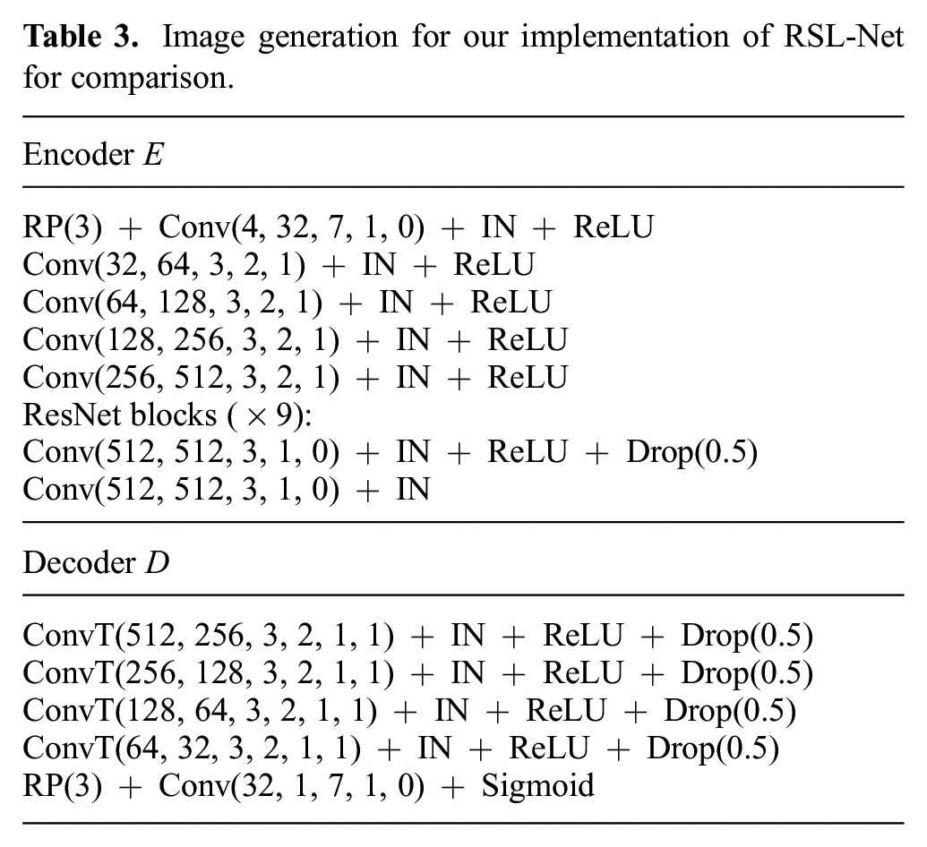
Image generation for our implementation of RSL-Net for comparison.
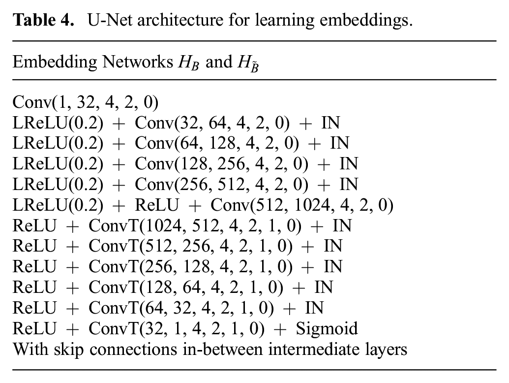
U-Net architecture for learning embeddings.
Our method is implemented in PyTorch (Paszke et al., 2019). For training rotation inference
6. Experimental validation
We evaluate on several public, real-world datasets collected with vehicles equipped with on-board range sensors. The datasets we use come with metric ground truths that are decently accurate, though we noticed the GPS/INS solutions in certain places can drift up to a few meters.
We add large artificial pose offsets to the ground truth when querying for a satellite image, thereby simulating a realistic robot navigation scenario where the initial pose estimate can solve place recognition, but is too coarse for the robot’s metric pose. Using a map (e.g., satellite) image queried at this coarse initial pose estimate, our method solves metric localization by comparing against the live sensor data. The true pose offsets are hidden during training as our method is self-supervised, and are only revealed at test time for evaluation purposes.
The artificial offset is chosen such that the initial estimate has an unknown heading error in the range
6.1. Radar localization against satellite imagery
We evaluate our method on two datasets with FMCW radar and GPS: the Oxford Radar RobotCar Dataset (Barnes et al., 2020) and the MulRan Dataset (Kim et al., 2020). The satellite images for RobotCar are queried using Google Maps Platform. 2 For MulRan they are queried using Bing Maps Platform, 3 as high-definition Google satellite imagery is unavailable at the place of interest.
The GPS/INS and range sensor data for all datasets used are timestamped. To create the ground truth, for each frame of range sensor data, we find its associated latitude, longitude, and heading from the GPS/INS data based on the time-stamp, and query a satellite image with the corresponding latitude and longitude. We also rotate the range sensor image with the ground-truth heading to generate a rotation-aligned range sensor image. To add the initial offset for simulating a coarse initial estimate, we simply shift the center of the satellite images by the translation offset and rotate the range sensor image by the heading offset when forming the range sensor–satellite pairs.
We benchmark against the prior supervised method RSL-Net (Tang et al., 2020b) in our experiments, which is evaluated only on the RobotCar Dataset. Both datasets contain repeated traversals of the same routes. We separately train, validate, and test for every dataset, splitting the data as in Figure 12. For the RobotCar Dataset, we split the trajectories the same way as in Tang et al. (2020b) for a fair comparison. For the RobotCar Dataset, the training set consists of training data from sequences no. 2, no. 5, and no. 6, whereas we test on the test data from sequence no. 2. For the MulRan Dataset, we used sequences
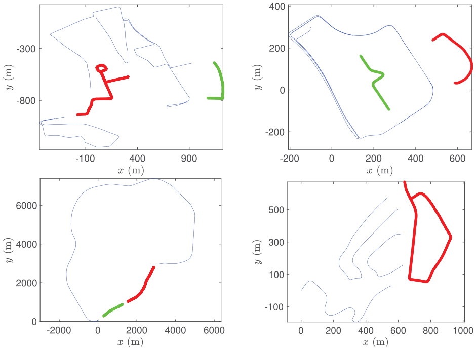
Training (blue), validation (green), and test (red) trajectories for RobotCar (top left),
We test on every fifth frame, resulting in 201 frames from the RobotCar Dataset and 358 from the MulRan Dataset, spanning a total distance of almost 4 km. The resolution used is
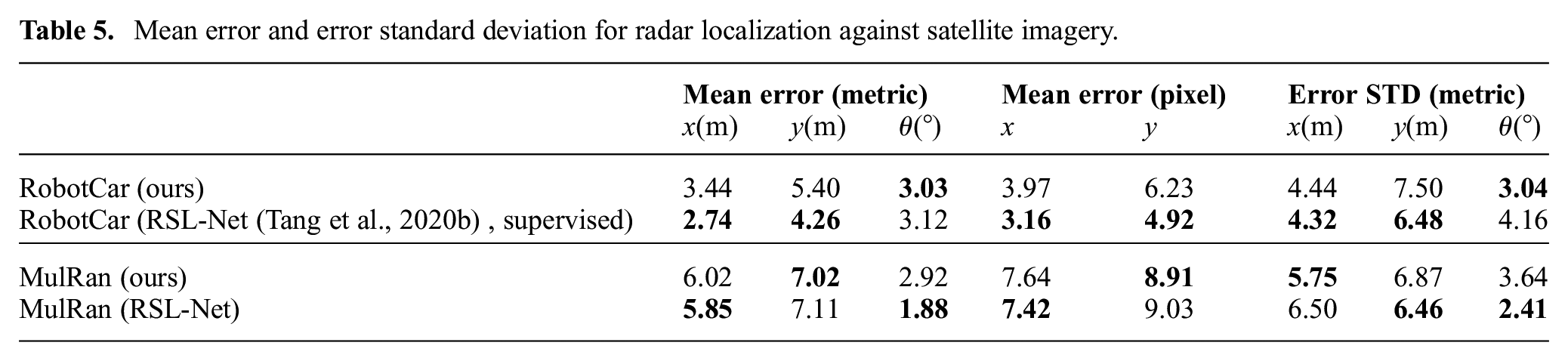
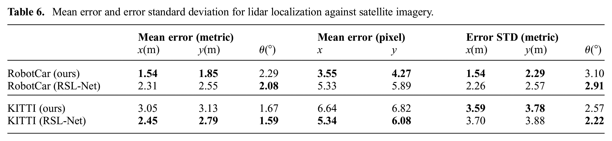
Mean error and error standard deviation for radar localization against satellite imagery.
6.2. Lidar localization against satellite imagery
For this experiment, we evaluate on the RobotCar Dataset (Barnes et al., 2020) which also has two Velodyne HDL-32E lidars mounted in a tilted configuration, and KITTI (raw dataset (Geiger et al., 2013)) which has a Velodyne HDL-64E lidar and GPS data.
For the RobotCar Dataset, the trajectories are split into training, validation, and test sets approximately the same way as in Section 6.1. For the KITTI Dataset, the training set includes sequences
As lidars have a shorter range than radars, we use satellite images of a greater zoom level, with resolution
Mean error and error standard deviation for lidar localization against satellite imagery.
6.3. Radar localization against prior lidar map
Though our method is designed for localizing against satellite imagery, we show it can also handle more standard forms of cross-modality localization. Here we build a lidar map using a prior traversal, and localize using radar from a later traversal.
We demonstrate on the RobotCar and MulRan datasets, where we use the same resolution as in Section 6.1. For RobotCar, we use ground truth to build a lidar map from sequence no. 2. Radar data in the training sections from no. 5 and no. 6 as in Figure 12 form the training set, whereas the test section from sequence no. 5 forms the test set. For MulRan, lidar maps are built from
Mean error and error standard deviation for radar localization against prior lidar map.
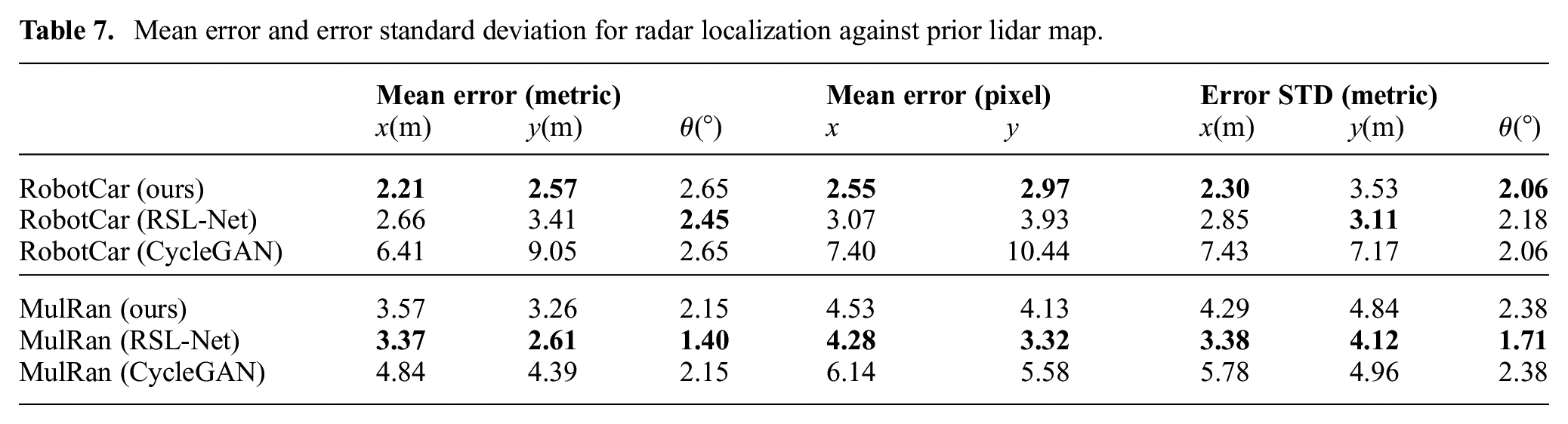
This experiment is more suitable for naive image generation methods such as CycleGAN (Zhu et al., 2017) than previous experiments, because the field of view is considerably more compatible as both modalities are from range sensors. In Table 7, we list results where we replaced the image generation stage of our method by CycleGAN while keeping other modules unchanged. The localization results are, however, much worse when modality
6.4. Online pose-tracking system
In prior experiments we assumed place recognition is always available, providing a coarse initial estimate for every frame. Here we present a stand-alone pose-tracking system by continuously localizing against satellite imagery. Given a coarse initial estimate (e.g., from GPS) for the first frame, the vehicle localizes and computes its pose within the satellite map. The initial estimate for every frame onward is then set to be the computed pose of the previous frame. We only need place recognition once at the very beginning; the vehicle then tracks its pose onward without relying on any other measurements.
6.4.1. Introspection
As localizing using satellite imagery is challenging, the result will not always be accurate. Our method, however, naturally allows for introspection. A synthetic image
Let
6.4.2. Results
We conduct two experiments on the test set of RobotCar, one where we track a radar using satellite imagery, and one where we track a lidar. For both experiments we run localization at 4 Hz. The results are shown in Figure 13. If the solution error is too large, then the initial estimate will be too off for a sufficient overlap between the next queried satellite image and live data, resulting in losing track of the vehicle. Although the solution error is large for certain frames, our system continuously localizes the vehicle for over a kilometer without completely losing track. For the lidar experiment, the solutions are sufficiently accurate to not require any odometry. Each solution only uses a single frame of data (plus the solution from the previous frame for the initial estimate), and we make no attempt at windowed/batch optimization or loop closures.
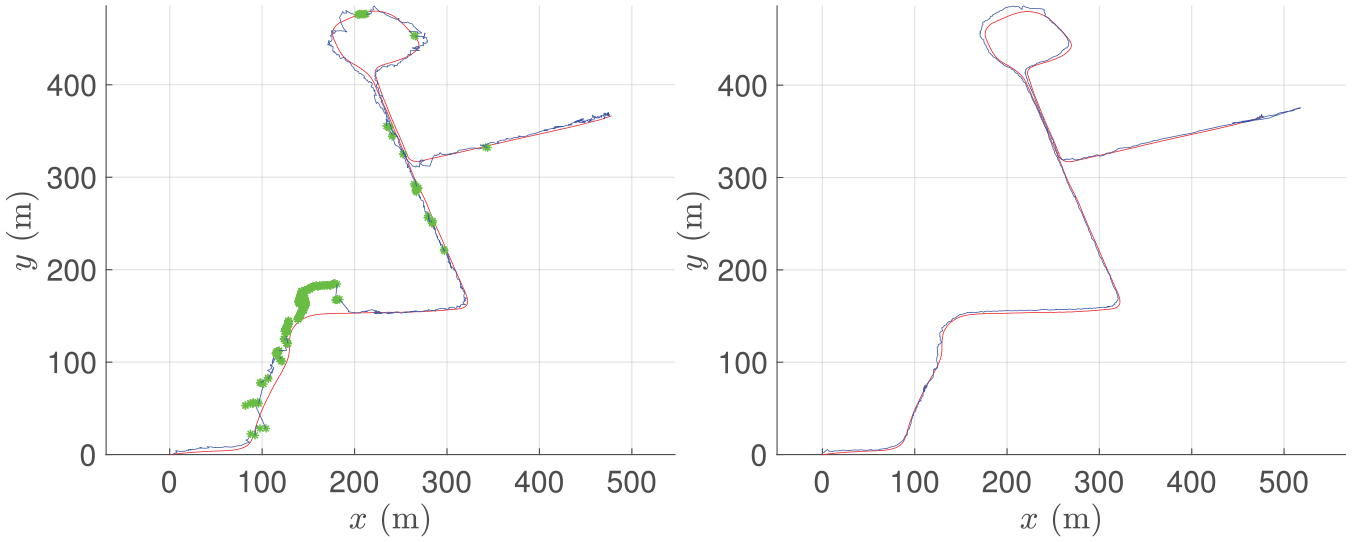
Estimated pose (blue) versus ground-truth pose (red) for localizing a radar (left) and a lidar (right) against satellite imagery. Our system tracks the vehicle’s pose over 1 km, where we occasionally fall back to odometry for the radar experiment (green). Our system is stand-alone and requires GPS only for the first frame.
6.5. Ablation study
We perform an ablation study to investigate the effect of reduced training data. For radar localization against satellite imagery on the RobotCar Dataset, we trained a model using approximately the first 20% of training data, and another using every
Ablation study for using reduced training data, evaluated on radar localization against satellite imagery on the RobotCar Dataset.
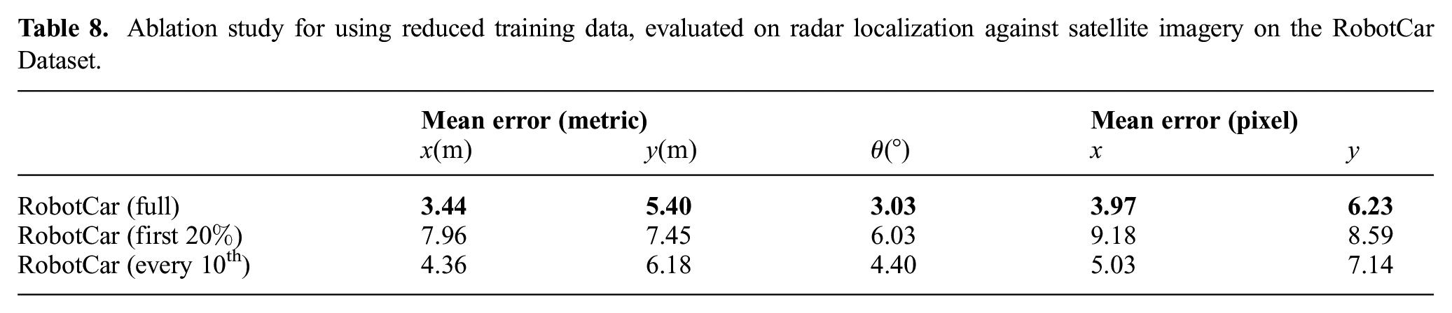
Noticeably, the choice of selecting uniformly distributed data in contrast to utilizing only the first 20% leads to a more varied dataset, and as such achieves better performances despite the lower number of samples.
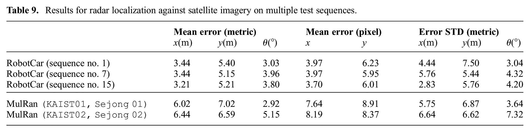
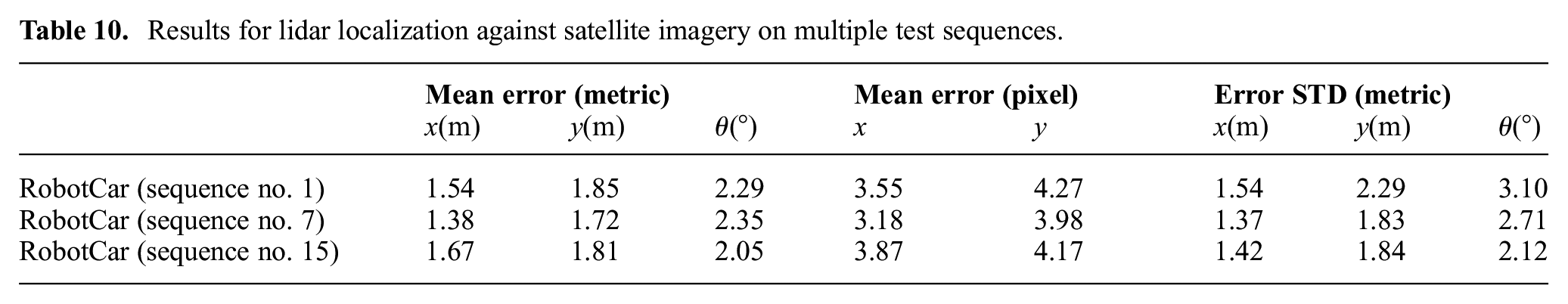
6.6. Testing on different sequences
For the results in Tables 5, 6, and 7, the training and test data, though with zero spatial overlap, are from the same sequences. The RobotCar and MulRan datasets contain repeated sequences of the same trajectory. Here we show results where the test set trajectories are from different sequences, to demonstrate the capability of generalizing not only to unseen places, but also to range sensor data recorded on different days as the training data.
We arbitrarily selected sequences no. 7 and no. 15 as the new test sequences for RobotCar, and sequences
The localization results are listed in Table 9 and Table 10. The mean errors are fairly consistent across different sequences.
Results for radar localization against satellite imagery on multiple test sequences.
Results for lidar localization against satellite imagery on multiple test sequences.
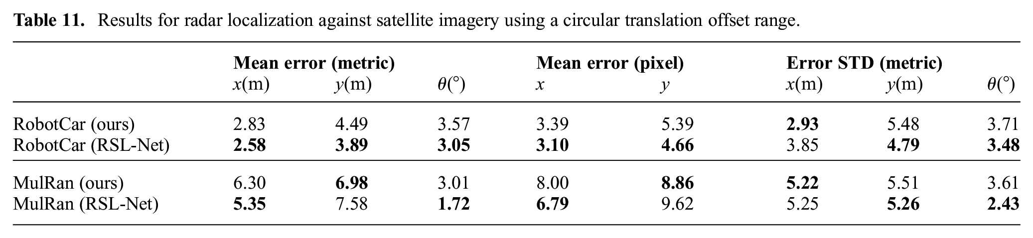
6.7. Circular initial offset
For a fair comparison against the supervised approach in Tang et al. (2020b), we assume the initial offset for both
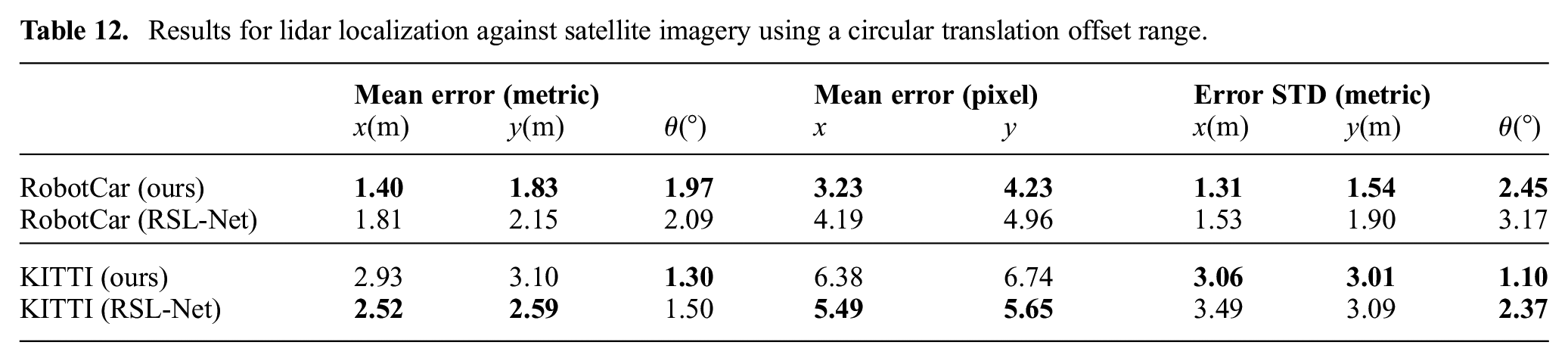
Without re-training, we evaluate the model performance where the initial translation offset is sampled uniformly from a circular area with a radius of 25 pixels, and centered at the ground truth position. The sampling for the initial heading offset remains unchanged. The localization results are summarized in Tables 11 and 12.
Results for radar localization against satellite imagery using a circular translation offset range.
Results for lidar localization against satellite imagery using a circular translation offset range.
6.8. Trade-offs on network width and depth
Here we show the effects of network width (number of channels in each layer) and depth (number of layers) on solution quality and the associated trade-offs, and justify choosing the architecture shown in Tables 1 to 4. In this experiment, we vary the width or depth of networks for rotation inference and image generation, namely
Mean error for using various choices of network width and depth, evaluated on lidar localization against satellite imagery on the RobotCar Dataset.
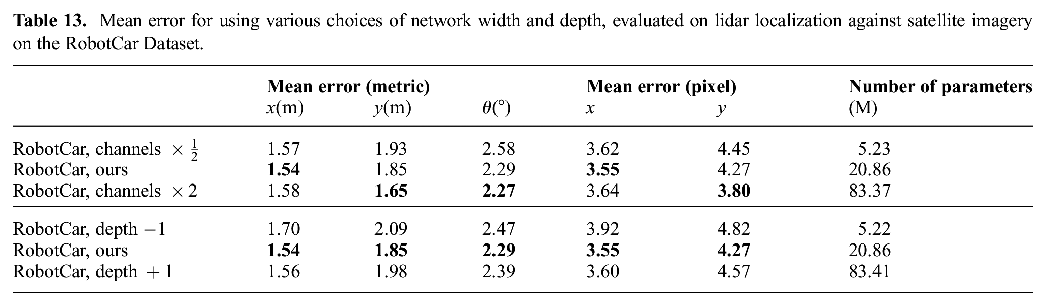
First, we fix the network depth while halving or doubling the number of channels in each layer. When the width is reduced, the network representation power is noticeably affected, indicated by an increase in solution error in all of
Next, we keep the number of channels the same in the first layer, and study the effect of making the networks shallower or deeper (by one layer). For image generation we use an encoder–decoder architecture with stride 2 in the convolution layers (after the first layer) as shown in Table 2, thus the height and width of the representation decrease by a factor of 2 after each layer, becoming
6.9. Choice of image resolution
In the results presented in Sections 6.1 and 6.2, we used a resolution of
To study the effect of image resolution on solution quality, we created another dataset for radar localization against satellite imagery from the RobotCar Dataset, where the resolution is set to be
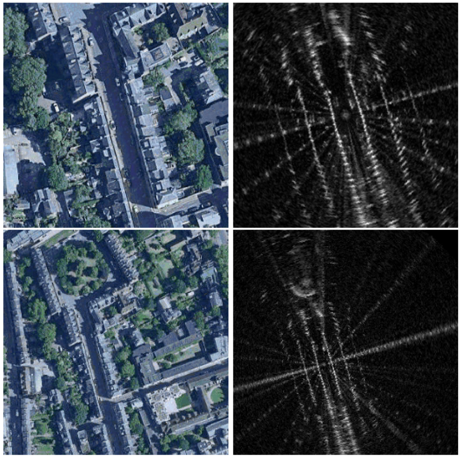
A pair of satellite and radar images queried using zoom levels of 18 (top) versus 17 (bottom) at roughly the same center position. Although “zooming in” can lead to a more refined resolution, certain regions far away are not seen in the resulting radar images, despite being observed by the sensor.
Mean error and error standard deviation for using refined resolution, evaluated for radar localization against satellite imagery. We also include results for a hybrid approach utilizing both resolutions..
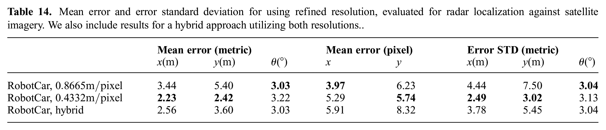
Overall, choosing a resolution of
Owing to the pixel-based nature of CNNs, the upper limit our method can handle in terms of initial translation offset is also inherently in pixels. Without changing the initial pose offset expressed in pixels, models trained with higher-resolution images offer a reduction in metric error, at the cost, however, of needing a smaller metric initial offset. In real-world applications, the coarse initial offset may be large, for example in places where direct GPS signals are occluded, and as such models trained with lower-resolution images are needed to handle such large initial offset. For a smaller metric initial offset, a model trained with higher-resolution images can be used to provide a more refined pose estimate.
With this in mind, we present a “hybrid” approach that utilizes both lower and higher resolution images. Specifically, given an initial offset in the range
6.10. Choice of rotation increment
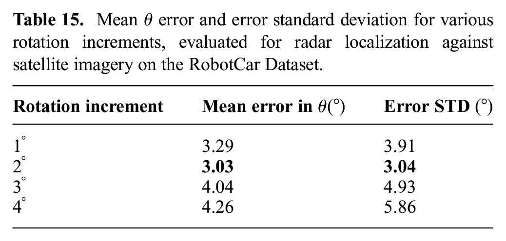
We have chosen a rotation increment of
By intuition, the solution error on
As listed in Table 15, the mean error in
Mean
6.11. Handling larger initial offset
So far, all experiments presented start from an initial translation offset of
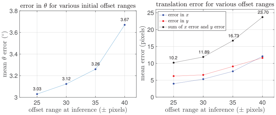
Mean error in rotation (left) and translation (right) with larger initial translation offset range, evaluated for radar localization against satellite imagery on the RobotCar Dataset.
Our method, however, naturally allows for a strategy to deal with larger initial offsets at inference time than in the training data, without the need to re-train. At inference, rather than using just
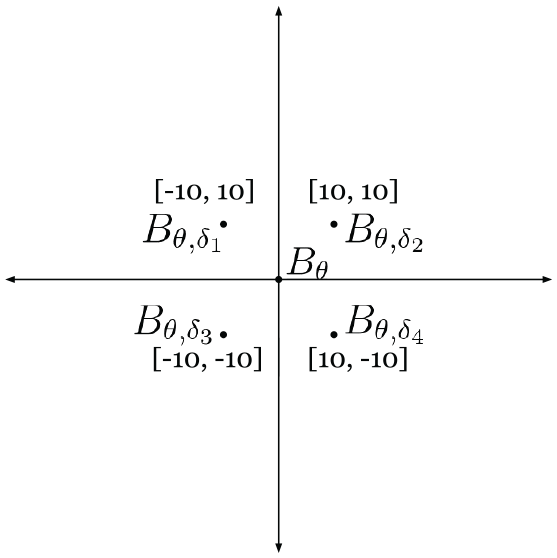
The center of image
Figure 17 depicts a case where the translation offset
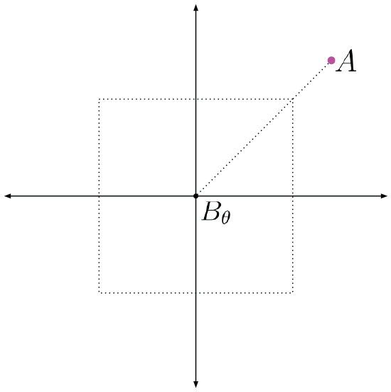
The unknown translation offset
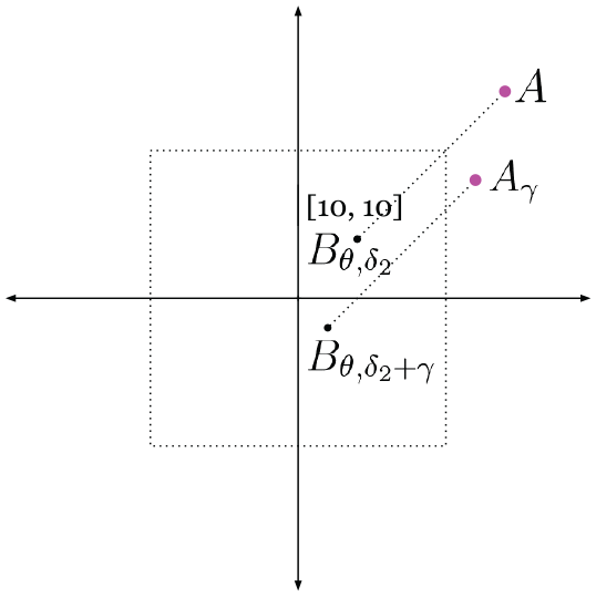
If we shift
Forming
It should be noted that such a combination does not suffer from the issue with large offsets, as discussed.
The remaining question is then which shifted image from
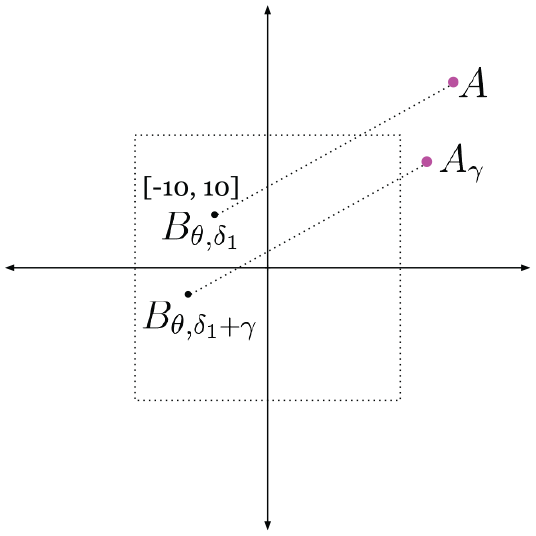
The resulting synthetic image will still be erroneous, if an incorrect quadrant is selected. Here the offset between
We can generate five versions of
For each shift
For each shift
along with an error term
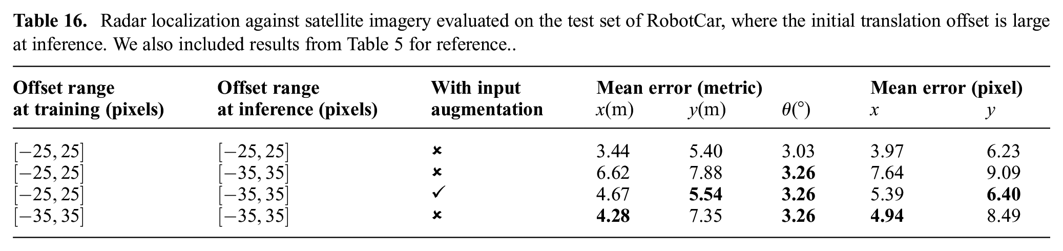
Table 16 shows results on the RobotCar Dataset for radar localization against satellite imagery, where the initial offset is now in the range of
Radar localization against satellite imagery evaluated on the test set of RobotCar, where the initial translation offset is large at inference. We also included results from Table 5 for reference..
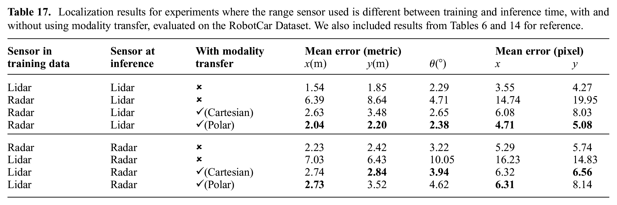
6.12. Modality transfer
An interesting application would be to train models using data for localization between one type of range sensor (e.g., radar) and satellite imagery, and evaluate for localization between another type of range sensor (e.g., lidar) and satellite imagery. This is particularly useful if we wish to evaluate using a specific type of range sensor at inference, but do not have the associated training data with approximately known trajectories to query for satellite images.
Here we demonstrate how this can be achieved using unsupervised domain adaptation by image-to-image transfer. Specifically, we consider CycleGAN (Zhu et al., 2017) for transferring between radar scan images and lidar scan images. For transferring between images of single scans of radar and lidar data, we also implement the approach in Weston et al. (2020), where range sensor data are converted into polar coordinate representation prior to the domain adaptation. Figure 20 shows examples of radar and lidar images and their synthetic counterparts generated using our implementation of CycleGAN, for both polar and Cartesian coordinate representations.
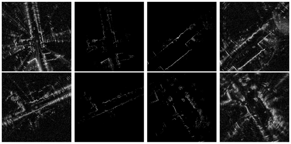
Qualitative results of CycleGAN for domain adaptation between a single scan of radar and lidar data. From left to right: a real radar image and its synthetic lidar image, a real lidar image and its synthetic radar image. Top: CycleGAN applied in Cartesian coordinate representation. Bottom: CycleGAN applied in polar coordinate representation.
At inference, given networks
We can then use
The same can be performed for the other way around, where given networks trained for lidar localization against satellite imagery, we wish to perform radar localization against satellite imagery at inference time.
Table 17 summarizes the results for modality transfer. Networks trained with one type of range sensor suffer from large localization errors when directly evaluated with another type of sensor. The errors are greatly reduced after applying domain adaptation and using transferred images as input. As shown in Figure 20, applying domain adaptation in polar coordinate representation led to more visually realistic synthetic images when transferring from lidar to radar data, and the smallest localization errors for networks trained on radar data and tested with lidar data. Applying domain adaptation in Cartesian coordinate representation, on the other hand, resulted in smaller errors for the reverse experiment. We use radar and lidar images of the same resolution in this experiment, and do not consider modality transfers that also involve a change in resolution.
6.13. Further qualitative results
Additional qualitative results are presented in Figure 21 showing various stages of our methods for different modalities and datasets.
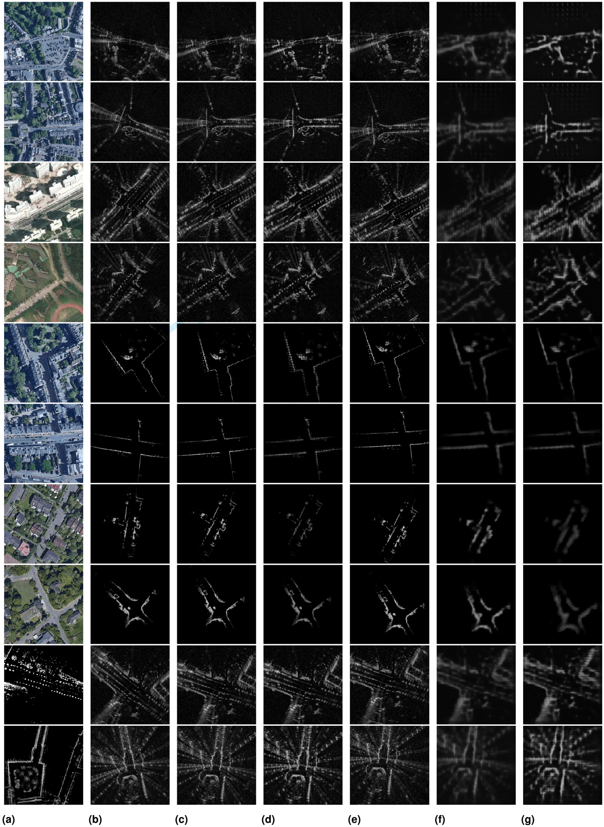
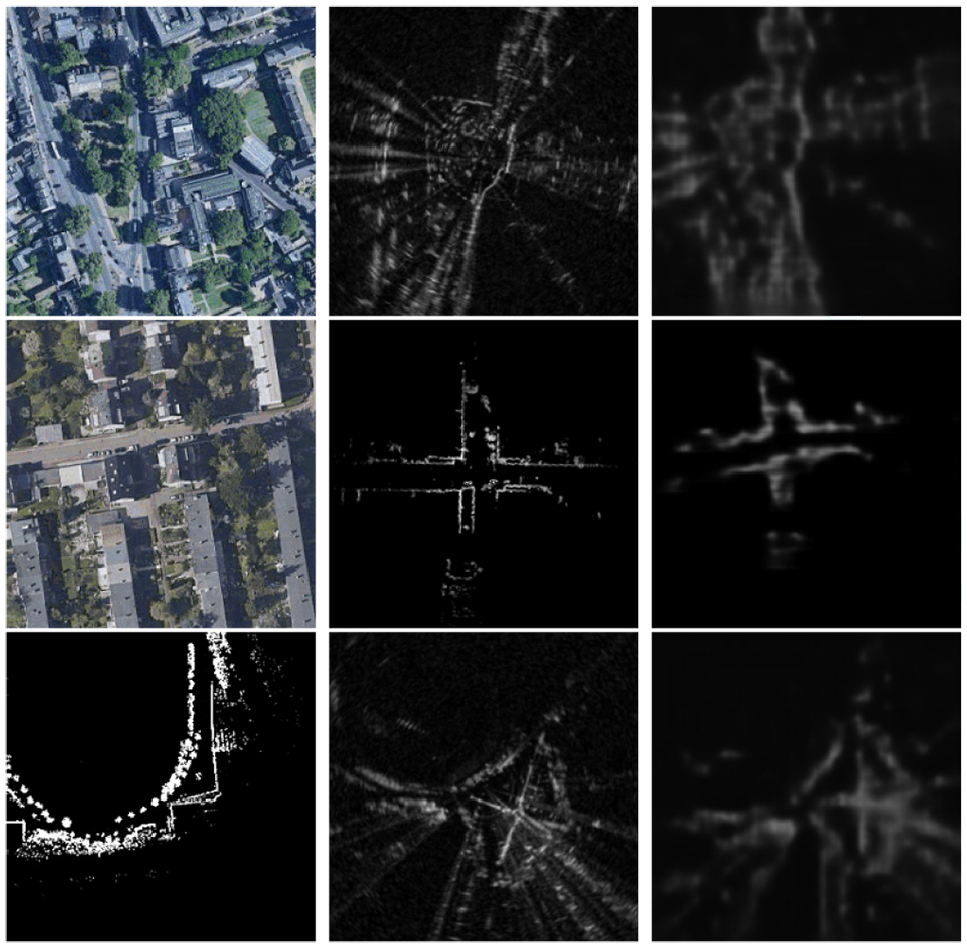
Images at various stages of our method: map image
7. Conclusion and future work
We present self-supervised learning to address cross-modality, metric localization between satellite imagery and on-board range sensors, without metrically accurate ground truth for training. Our approach utilizes a multi-stage network that solves for the rotation and translation offsets separately through the generation of synthetic range sensor images as an intermediate step. Our method is validated across a large number of experiments for multiple modes of localization, with results on par with a prior supervised approach. A coarse initial pose estimate is needed for our method to compute metric localization. Therefore, a natural extension would then be to solve place recognition for a range sensor within a large satellite map as a prior step to metric localization.
Footnotes
Acknowledgements
We thank Giseop Kim from IRAP Lab, KAIST for providing GPS data for the MulRan Dataset.
Funding
The work of Tim Y. Tang was jointly supported by a Postgraduate Scholarship - Doctoral Program (PGS-D) from the Natural Sciences and Engineering Research Council of Canada, and an Oxford Robotics Institute Studentship. The work of Daniele De Martini and Paul Newman were supported by the EPSRC (Programme Grant EP/M019918/1: “Mobile Robotics: Enabling a Pervasive Technology of the Future”). The work of Shangzhe Wu was supported by Facebook Research.