
Abstract
We use reinforcement learning (RL) to learn dexterous in-hand manipulation policies that can perform vision-based object reorientation on a physical Shadow Dexterous Hand. The training is performed in a simulated environment in which we randomize many of the physical properties of the system such as friction coefficients and an object’s appearance. Our policies transfer to the physical robot despite being trained entirely in simulation. Our method does not rely on any human demonstrations, but many behaviors found in human manipulation emerge naturally, including finger gaiting, multi-finger coordination, and the controlled use of gravity. Our results were obtained using the same distributed RL system that was used to train OpenAI Five. We also include a video of our results: https://youtu.be/jwSbzNHGflM.
Keywords
1. Introduction
While dexterous manipulation of objects is a fundamental everyday task for humans, it is still challenging for autonomous robots. Modern-day robots are typically designed for specific tasks in constrained settings and are largely unable to utilize complex end-effectors. In contrast, people are able to perform a wide range of dexterous manipulation tasks in a diverse set of environments, making the human hand a grounded source of inspiration for research into robotic manipulation.
The Shadow Dexterous Hand (ShadowRobot, 2005) is an example of a robotic hand designed for human-level dexterity; it has five fingers with a total of 24 degrees of freedom (DoFs). The hand has been commercially available since 2005; however, it still has not seen widespread adoption, which can be attributed to the daunting difficulty of controlling systems of such complexity. The state-of-the-art in controlling five-fingered hands is severely limited. Some prior methods have shown promising in-hand manipulation results in simulation but do not attempt to transfer to a real-world robot (Bai and Liu, 2014; Mordatch et al., 2012). Conversely, owing to the difficulty in modeling such complex systems, there has also been work in approaches that only train on a physical robot (Falco et al., 2018; Kumar et al., 2016a,b; van Hoof et al., 2015). However, because physical trials are so slow and costly to run, the learned behaviors are very limited.
In this work, we demonstrate methods to train control policies that perform in-hand manipulation and deploy them on a physical robot. The resulting policy exhibits unprecedented levels of dexterity and naturally discovers grasp types found in humans, such as the tripod, prismatic, and tip pinch grasps, and displays contact-rich, dynamic behaviors such as finger gaiting, multi-finger coordination, the controlled use of gravity, and coordinated application of translational and torsional forces to the object. Figure 1 depicts an exemplary manipulation sequence. Our policy can also use vision to sense an object’s pose: an important aspect for robots that should ultimately work outside of a controlled lab setting.
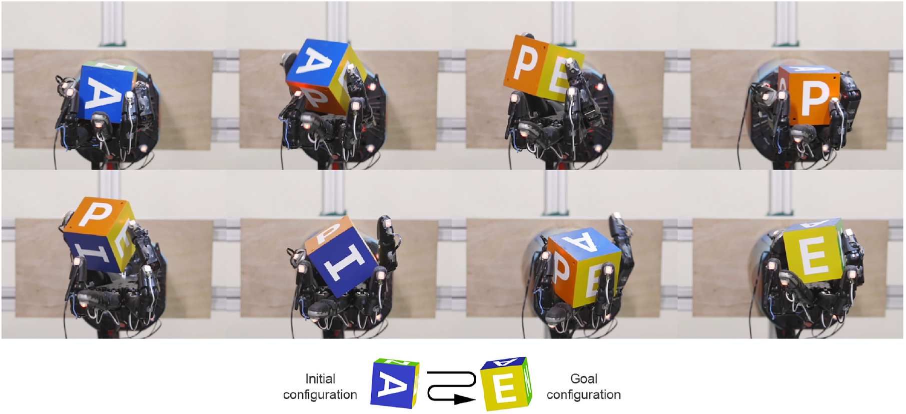
A five-fingered humanoid hand trained with reinforcement learning manipulating a block from an initial configuration to a goal configuration using vision for sensing.
Despite training entirely in a simulator that substantially differs from the real world, we obtain control policies that perform well on the physical robot. We attribute our transfer results to (1) extensive randomizations and added effects in the simulated environment alongside calibration, (2) memory augmented control polices that admit the possibility to learn adaptive behavior and implicit system identification on the fly, and (3) training at large scale with distributed reinforcement learning (RL). An overview of our approach is depicted in Figure 2.
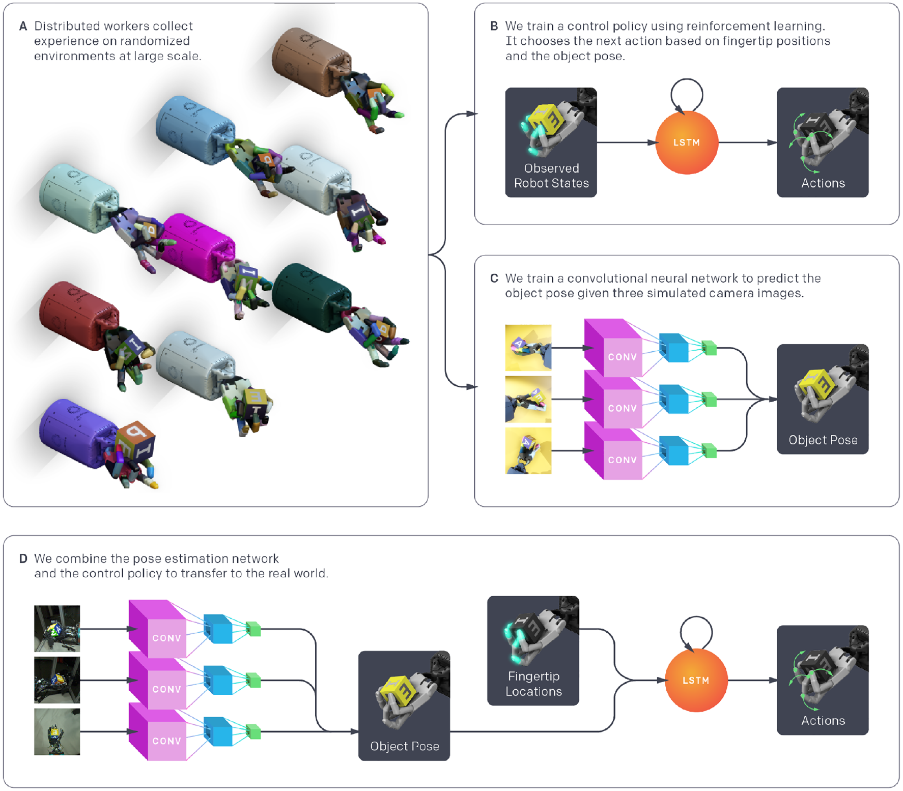
System overview. (a) We use a large distribution of simulations with randomized parameters and appearances to collect data for both the control policy and vision-based pose estimator. (b) The control policy receives observed robot states and rewards from the distributed simulations and learns to map observations to actions using a recurrent neural network and RL. (c) The vision-based pose estimator renders scenes collected from the distributed simulations and learns to predict the pose of the object from images using a convolutional neural network (CNN), trained separately from the control policy. (d) To transfer to the real world, we predict the object pose from three real camera feeds with the CNN, measure the robot fingertip locations using a 3D motion capture system, and give both of these to the control policy to produce an action that gets executed on the physical robot.
The paper is structured as follows. In Section 2 we briefly introduce the most important RL concepts and algorithms used in this work. Section 3 gives a system overview, describes the proposed task in more detail, and shows the hardware setup. Section 4 describes observations for the control policy, environment randomizations, and additional effects added to the simulator that make transfer possible. Section 5 outlines the control policy training procedure and our distributed RL system. Section 6 describes the vision model architecture and training procedure. Section 7 describes both qualitative and quantitative results from deploying the control policy and vision model on a physical robot. Section 8 discusses related work and we conclude with Section 9.
2. Background
In this section, we introduce the most fundamental RL concepts and discuss the algorithms that we use in this work. For an in-depth introduction to RL, please refer to Sutton and Barto (1998) and Bertsekas (2005).
2.1. RL
We consider the standard RL formalism consisting of an agent interacting with an environment. To simplify the exposition, we assume in this section that the environment is fully observable.
1
An environment is described by a set of states
A policy
The Q-function or action-value function is defined as
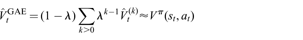
2.2. Generalized advantage estimator
Let V be an approximator to the value function of some policy, i.e.,
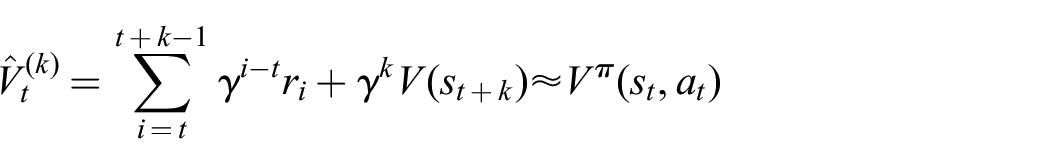
is called the k-step return estimator. The parameter k controls the bias–variance tradeoff of the estimator with bigger values resulting in an estimator closer to empirical returns and having less bias and more variance. The generalized advantage estimator (GAE) (Schulman et al., 2015) is a method of combining multi-step returns in the following way:
where

It is possible to compute the values of this estimator for all states encountered in an episode in linear time (Schulman et al., 2015).
2.3. Proximal policy optimization
Proximal policy optimization (PPO) (Schulman et al., 2017) is one of the most popular on-policy RL algorithms. It simultaneously optimizes a stochastic policy as well as an approximator to the value function. PPO interleaves the collection of new episodes with policy optimization. After a batch of new transitions is collected, optimization is performed with minibatch stochastic gradient descent to maximize the objective:
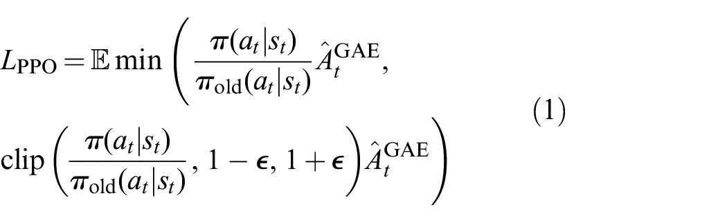
where
The value function approximator is trained with supervised learning with the target for
3. Task and system overview
In this work, we consider the problem of in-hand object reorientation. We place the object under consideration onto the palm of a humanoid robot hand. The goal is to reorient the object to a desired target configuration in-hand. As soon as the current goal is (approximately) achieved, a new goal is provided until the object is eventually dropped. We use two different objects, a block and an octagonal prism.
This section first describes our hardware setup in detail and then describes how we model the task in simulation.
3.1. Hardware
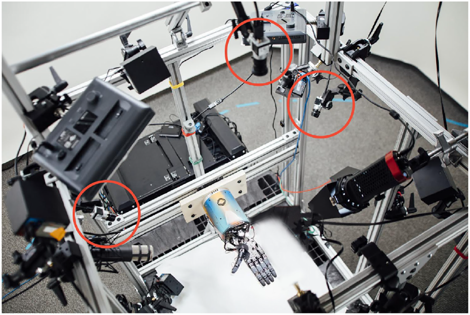
Our hardware setup consists of a Shadow Dexterous Hand, a PhaseSpace tracking system, as well as a RGB camera system for vision. The entire setup is depicted in Figure 3.

The “cage” that houses the robot hand, 16 PhaseSpace tracking cameras, and 3 Basler RGB cameras.
3.1.1. Shadow Dexterous Hand
We use the Shadow Dexterous Hand, which is a humanoid robotic hand with
3.1.2. PhaseSpace tracking
We use a 3D tracking system to localize the tips of the fingers, to perform calibration procedures, and as ground truth for the RGB image-based object tracking. The PhaseSpace Impulse X2E tracking system uses active LED markers that blink to transmit a unique ID code and linear detector arrays in the cameras to detect the positions and IDs. The system features capture speeds of up to 960 Hz and positional accuracies of below 20
3.1.3. RGB cameras
For estimating the pose of the object that the hand is manipulating, we have two setups: one that uses PhaseSpace markers to track the object (described above) and one that uses three Basler RGB cameras for vision-based pose estimation. This is because our goal is to eventually have a system that works outside of a lab environment, and vision-based systems are better equipped to handle the real world.
Each Basler acA640-750uc RGB camera has a resolution of
Our three-camera setup for vision-based state estimation.
3.1.4. Control
The high-level controller is implemented as a Python program running a neural network policy using Tensorflow (Abadi et al., 2016) on a GPU. Every
The low-level controller is implemented in C++ as a separate process on a different machine that is connected to the Shadow hand via an Ethernet cable. The controller is written as a real-time system: it is pinned to a CPU core, has preallocated memory, and does not depend on any garbage collector to avoid non-deterministic delays. The controller receives the relative action, converts it into an absolute joint angle and clips to the valid range, then sets each component of the action as the target for a PD controller. Every
3.1.5. Joint sensor calibration
The hand contains 26 Hall effect sensors that sense magnetic field rotations along the joint axis. To transform the raw magnetic measurements from the Hall sensors into joint angles, we use a piecewise linear function interpolated from 3–5 truth points per joint. To calibrate this function, we initialize to the factory default created using physical calibration jigs. For further accuracy, we attach PhaseSpace markers to the fingertips, and minimize the error between the position reported by the PhaseSpace markers and the position estimated from the joint angles. We estimate these linear functions by minimizing the reprojection error with
3.2. Simulation
We simulate the physical system with the MuJoCo physics engine (Todorov et al., 2012) and we use Unity (Unity Technologies, 2005) to render the images for training the vision-based pose estimator. Our model of the Shadow Dexterous Hand is based on that used in the OpenAI Gym robotics environments (Brockman et al., 2016; Plappert et al., 2018), but has been improved to match the physical system more closely through calibration. A rendering of our simulation is depicted in Figure 5. In the remainder of this section, we describe all aspects of our simulation in detail.
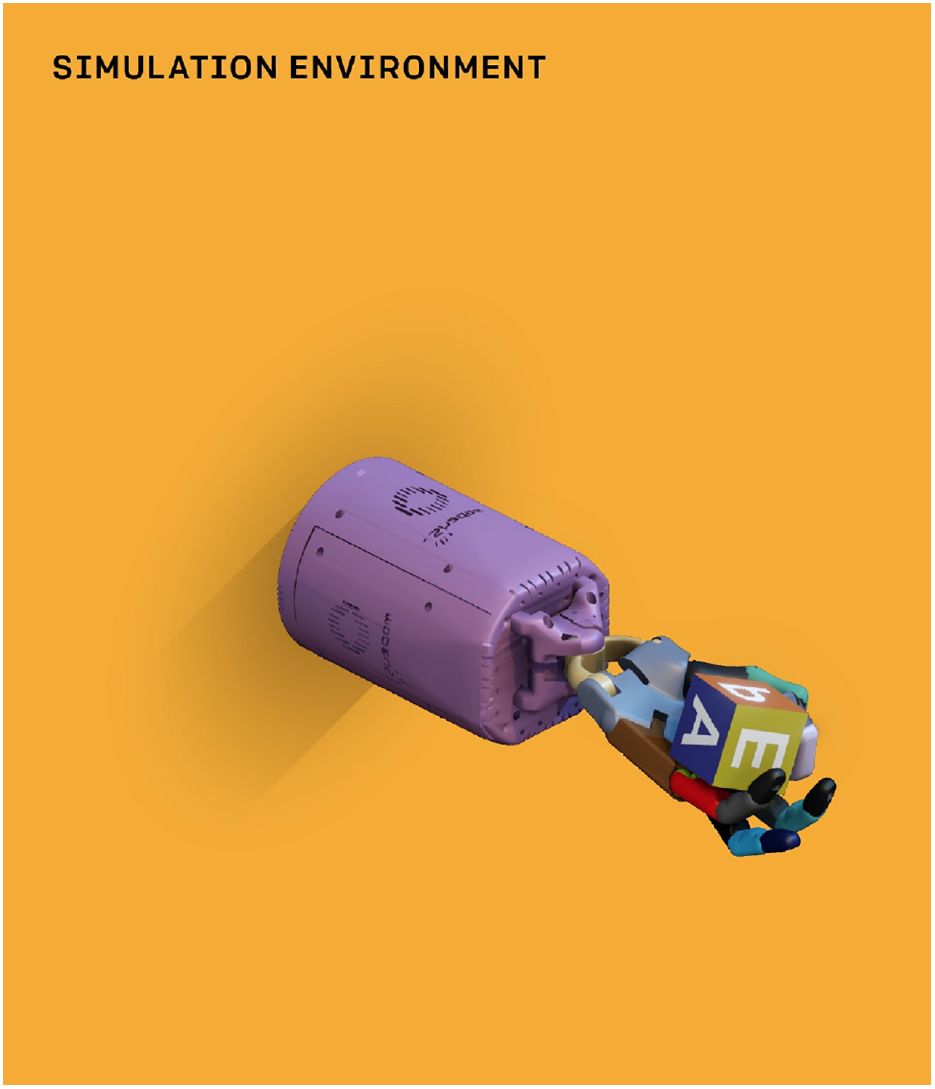
A rendering of our simulated environment.
3.2.1. States
The state of the system is 60-dimensional and consists of angles and velocities of all robot joints as well as the position, rotation, and velocities (linear and angular) of the object. Initial states are sampled by placing the object on the robot’s palm in a random orientation and applying random actions for
3.2.2. Goals
The goal is the desired orientation of the object represented as a quaternion. A new goal is generated after the current one has been achieved within a tolerance of 0.4 rad. We consider a goal achieved if there exists a rotation of the object around an arbitrary axis with an angle smaller than 0.4 rad which transforms the current orientation into the desired one.
3.2.3. Actions
Actions are 20-dimensional and correspond to the desired angles of the hand joints. We discretize each action coordinate into
All actions are rescaled to the range
3.2.4. Rewards
The reward given at timestep t is
3.2.5. Timing
Each environment step corresponds to 80 ms of real time and consists of
3.2.6. Model calibration
We calibrate the parameters of our MuJoCo XML model to better match our physical setup. To do so, we record a trajectory on the physical robot and then optimize over parameters to minimize the error between the simulated and real trajectory.
To create the trajectory, we run two hand-designed policies in sequence against each finger. The first policy measures the behavior of the joints near their limits by extending the joints of each finger completely inward and then completely outward until they stop moving. The second policy measures the dynamic response of the finger by moving the joints of each finger inward and then outward in a series of oscillations. The recorded trajectory across all fingers lasts a few minutes.
To optimize the model parameters, these trajectories are then replayed as open-loop action sequences in the simulator. The optimization objective is to match simulated and real joint angles after
4. Transferable simulations
Despite our calibration and modeling efforts, the simulation is still only a rough approximation of the physical setup. For example, our model directly applies torque to joints instead of tendon-based actuation and uses rigid-body contact models instead of deformable-body contact models even though the physical robot has deformable fingertips made out of rubber. These differences cause a “reality gap” and make it unlikely for a policy trained in a simulation with these inaccuracies to transfer well.
We therefore face a dilemma: we cannot train on the physical robot because deep RL algorithms require millions of samples; conversely, training only in simulation results in policies that do no transfer well due to the gap between the simulated and real environments. To overcome the reality gap, we modify the basic version of our simulation to a distribution over many simulations that foster transfer (Peng et al., 2017; Sadeghi and Levine, 2017; Tobin et al., 2017a). By carefully selecting the sensing modalities and by randomizing most aspects of our simulated environment we are able to train policies that are less likely to overfit to a specific simulated environment and more likely to transfer successfully to the physical robot.
4.1. Observations
We give the control policy observations of the fingertips using PhaseSpace markers and the object pose either from PhaseSpace markers or the vision-based pose estimator. Although the Shadow Dexterous Hand contains a broad array of built-in sensors, we specifically avoided providing these as observations to the policy because they are subject to state-dependent noise that would have been difficult to model in the simulator. For example, the fingertip tactile sensor measures the pressure of a fluid stored in a balloon inside the fingertip, which correlates with the force applied to the fingertip but also with a number of confounding variables, including atmospheric pressure, temperature, and the shape of the contact and intersection geometry. Although it is straightforward to determine the existence of contacts in the simulator, it would be difficult to model the distribution of sensor values. Similar considerations apply to the joint angles measured by Hall effect sensors, which are used by the low-level controllers but not provided to the policy due to their tendency to be noisy and hard to calibrate.
4.2. Randomizations
Following previous work on domain randomization (Peng et al., 2017; Sadeghi and Levine, 2017; Tobin et al., 2017a), we randomize most of the aspects of the simulated environment in order to learn both a policy and a vision model that generalizes to reality. We overall found that it is important to center randomized parameters on reasonable physical values of the actual setup, which we obtain via the previously described calibration step. Randomizations also allow us to model uncertainty: we typically randomize parameters with high uncertainty (e.g., actuation parameters) more than parameters for which we have values with low uncertainty (e.g., object dimensions).
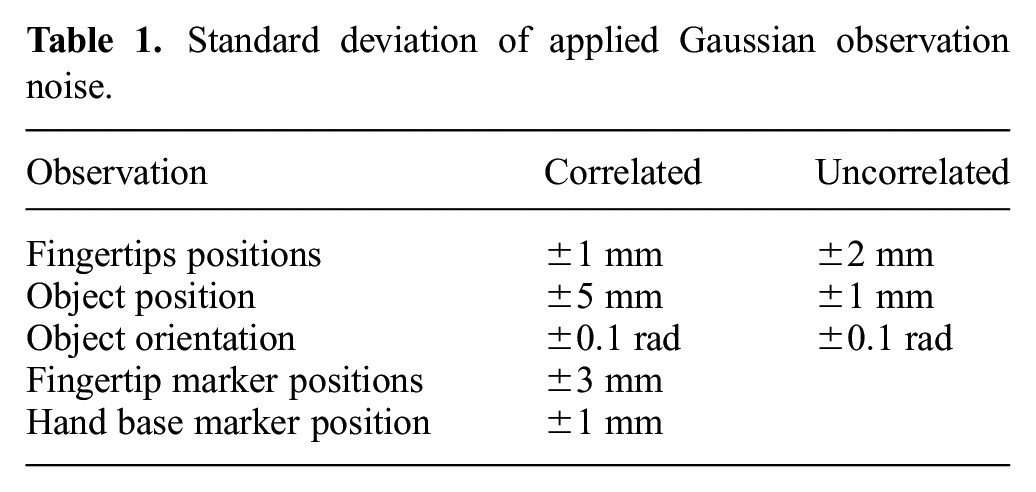
4.2.1. Observation noise
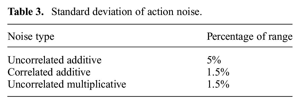
To better mimic the kind of noise we expect to experience in reality, we add Gaussian noise to policy observations. In particular, we apply a correlated noise that is sampled once per episode as well as an uncorrelated noise sampled at every timestep. Apart from Gaussian correlated noise, we also add more structured noise coming from inaccurate placement of the motion capture markers by computing the observations using slightly misplaced markers in the simulator. The configuration of noise levels is described in Table 1.
Standard deviation of applied Gaussian observation noise.
4.2.2. Physics randomizations
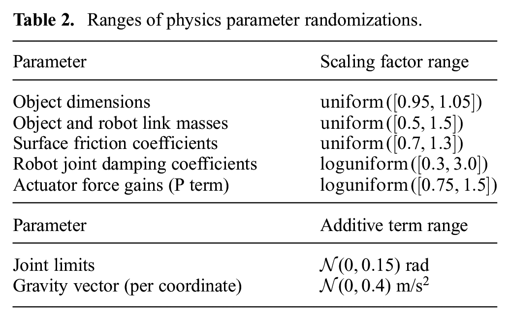
The physical parameters are sampled at the beginning of every episode and held fixed for the whole episode. We typically randomize around values that we obtained through calibration. The full set of randomized values are available in Table 2.
Ranges of physics parameter randomizations.
We also randomize the timing of environment steps. Every environment step is simulated as
4.2.3. Unmodeled effects
The physical robot experiences many effects that are not modeled by our simulation, e.g., motor backlash or motion capture occlusions. Here, we briefly describe each randomization.
Standard deviation of action noise.
4.2.4. Visual appearance randomizations
We randomize the following aspects of the rendered scene: camera positions and intrinsics, lighting conditions, the pose of the hand and object, and the materials and textures for all objects in the scene. Figure 6 depicts some examples of these randomized environments.
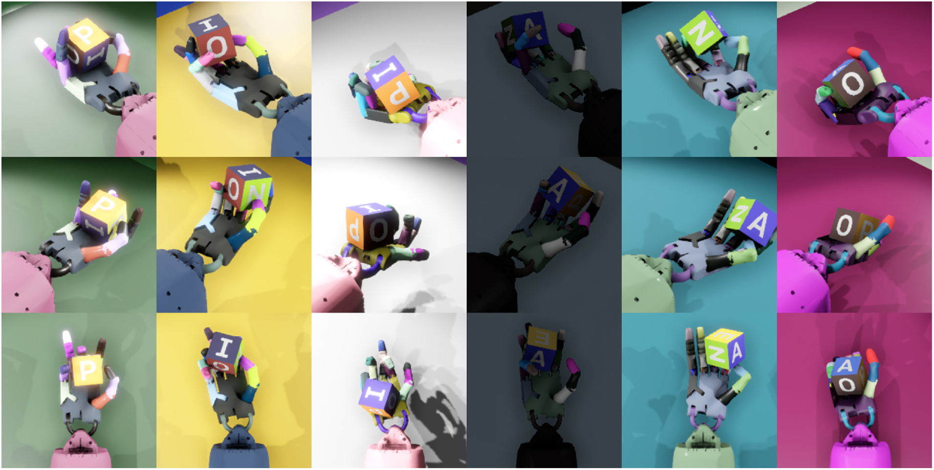
Simulations with different randomized visual appearances. Rows correspond to the renderings from the same camera, and columns correspond to renderings from three separate cameras that are simultaneously fed into the neural network.
The materials and textures are randomized for every visible object in the scene. We randomize the hue, saturation, and value for the object faces around calibrated values from real-world measurements. The color of the robot is uniformly randomized. Material properties such as glossiness and shininess are randomized as well. Camera position and orientation are slightly randomized around values calibrated to real-world locations. Lights are randomized individually, and intensities are scaled based on a randomly drawn total intensity. After rendering the scene to images from the three separate cameras, additional augmentation is applied. The images are linearly normalized to have zero mean and unit variance. Then the image contrast is randomized, and finally per-pixel Gaussian noise is added. Details are given in Table 4.
Ranges of vision randomizations.
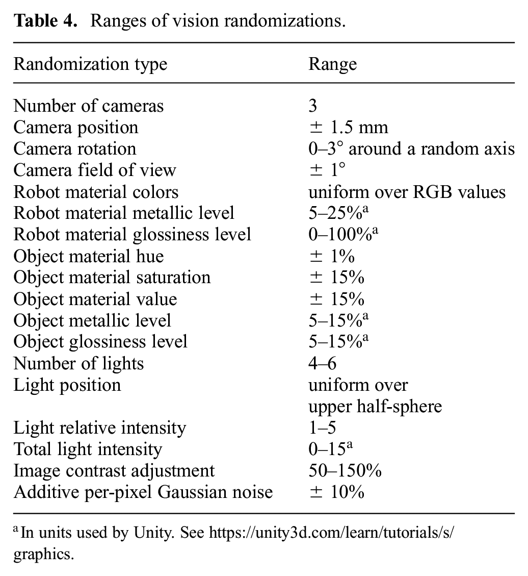
In units used by Unity. See https://unity3d.com/learn/tutorials/s/graphics.
5. Learning control policies from state
We use the previously described distribution over randomized simulations to train a single control policy using RL. Since we optimize for performance over all randomizations, the policy cannot overfit to a single variant of our simulation, thus making it transferable to the physical robot. However, since the policy has to handle a large number of different variants of the same problem, we propose to use a recurrent policy with access to memory. We further use a distributed RL system in order to make solving this challenging problem tractable. Both the policy architecture and our training procedure using our distributed system are described in this section.
5.1. Policy architecture
Many of the randomizations we employ persist across an episode, and thus it should be possible for a memory augmented policy to identify properties of the current environment and adapt its own behavior accordingly. For instance, initial steps of interaction with the environment can reveal the weight of the object or how fast the index finger can move. We therefore represent the policy as a recurrent neural network with memory, namely an LSTM (Hochreiter and Schmidhuber, 1997) with an additional hidden layer with ReLU (Nair and Hinton, 2010) activations inserted between inputs and the LSTM.
The policy is trained with PPO (Schulman et al., 2017). PPO requires the training of two networks: a policy network, which maps observations to actions; and a value network, which predicts the discounted sum of future rewards starting from a given state. Both networks have the same architecture but have independent parameters. The network architecture is depicted in Figure 7.
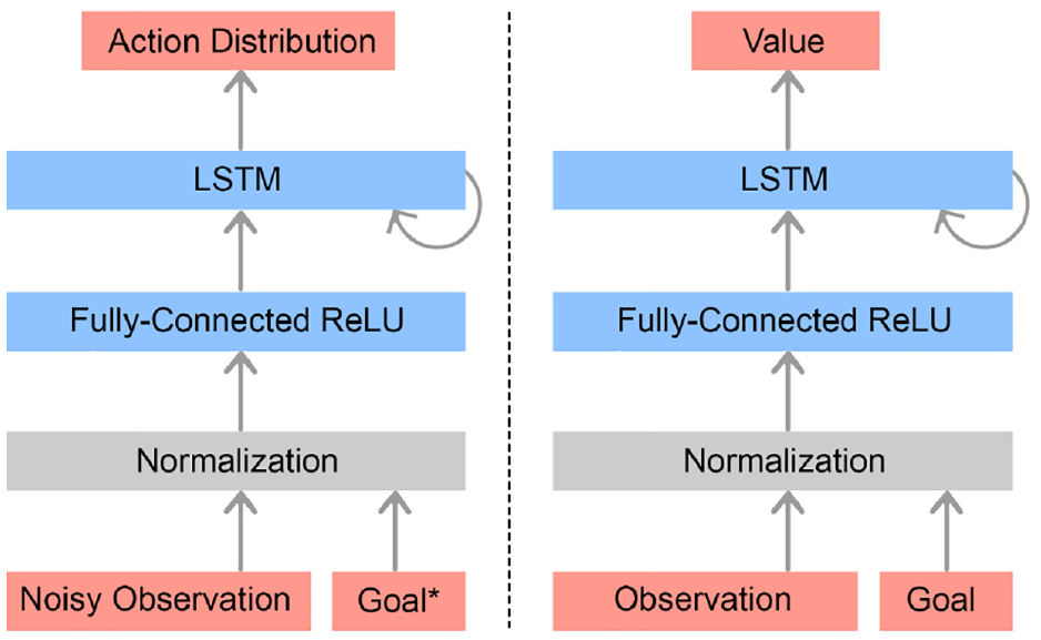
Policy network (left) and value network (right). Each network consists of an input normalization, a single fully connected hidden layer with 1,024 units and ReLU activations (Nair and Hinton, 2010), and a recurrent LSTM block (Hochreiter and Schmidhuber, 1997) with
Since the value network is only used during training, we use an Asymmetric Actor–Critic (Pinto et al., 2017a) approach. Asymmetric Actor–Critic exploits the fact that the value network can have access to information that is not available on the real robot system. This includes noiseless observation and additional observations such as joint angles and angular velocities, which we cannot sense reliably but which are readily available in simulation during training. The additional input potentially simplifies the problem of learning good value estimates since less information needs to be inferred.
We also normalize all observations given to the policy and value networks with running means and standard deviations. We then clip observations such that they are within five standard deviations of the mean. We normalize the advantage estimates within each minibatch. We also normalize targets for the value function with running statistics. The list of inputs fed to both networks can be found in Table 5.
Observations of the policy and value networks, respectively. “Noisy” means that observation noise has been applied as described in Section 4.
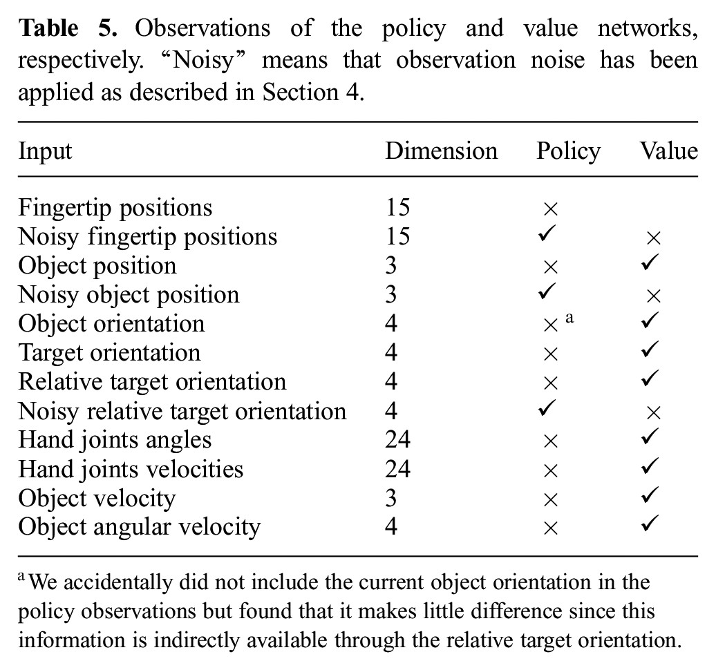
We accidentally did not include the current object orientation in the policy observations but found that it makes little difference since this information is indirectly available through the relative target orientation.
5.2. Distributed training with Rapid
We use the same distributed implementation of PPO that was used to train OpenAI Five (OpenAI, 2018) without any modifications. Overall, we found that PPO scales up easily and requires little hyperparameter tuning. The architecture of our distributed training system is depicted in Figure 8.
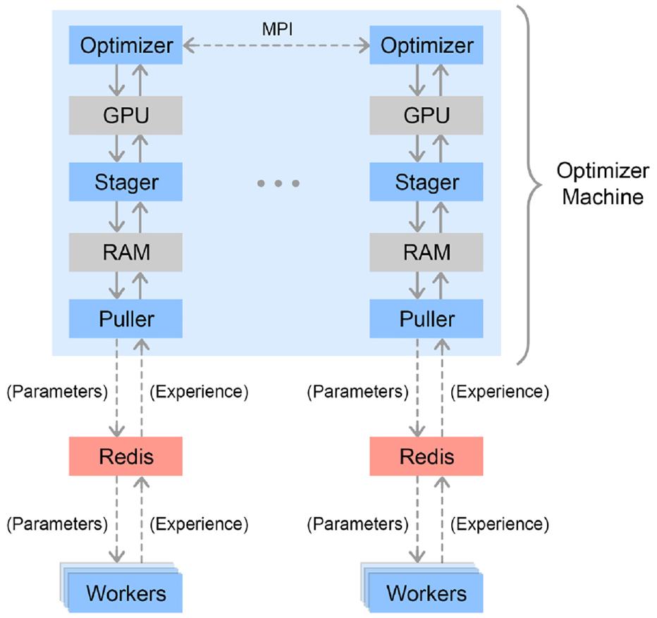
Our distributed training infrastructure in Rapid. Individual threads are depicted as blue squares. Worker machines randomly connect to a Redis server from which they pull new policy parameters and to which they send new experience. The optimizer machine has one MPI process for each GPU, each of which gets a dedicated Redis server. Each process has a Puller thread which pulls down new experience from Redis into a buffer. Each process also has a Stager thread which samples minibatches from the buffer and stages them on the GPU. Finally, each Optimizer thread uses a GPU to optimize over a minibatch after which gradients are accumulated across threads and new parameters are sent to the Redis servers.
In our implementation, a pool of
The optimization is performed on a single machine with eight GPUs. The optimizer threads pull down generated experience from Redis and then stage it to their respective GPU’s memory for processing. After computing gradients locally, they are averaged across all threads using MPI, which we then use to update the network parameters.
The hyperparameters that we used can be found in Table 6.
Hyperparameters used for PPO.
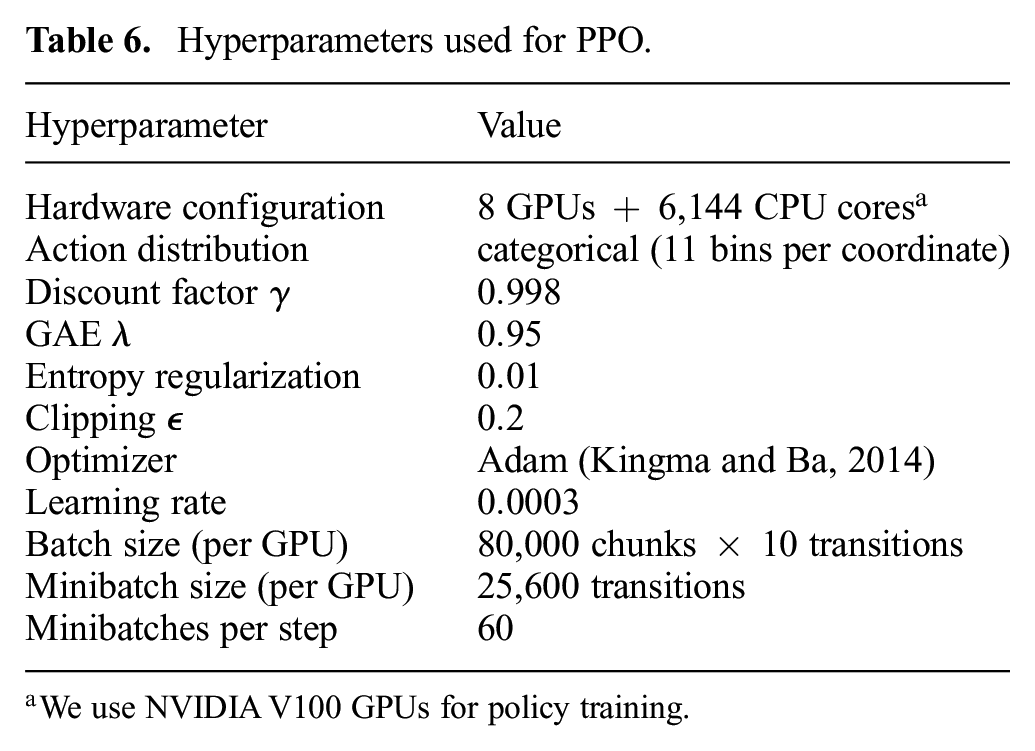
We use NVIDIA V100 GPUs for policy training.
6. State estimation from vision
The policy that we described in the previous section takes the object’s position as input and requires a motion capture system for tracking the object on the physical robot. This is undesirable because tracking objects with such a system is only feasible in a lab setting where markers can be placed on each object. Since our ultimate goal is to build robots for the real world that can interact with arbitrary objects, sensing them using vision is an important building block. In this work, we therefore wish to infer the object’s pose from vision alone. Similar to the policy, we train this estimator only on synthetic data coming from the simulator.
6.1. Model architecture
To resolve ambiguities and to increase robustness, we use three RGB cameras mounted with differing viewpoints of the scene. The recorded images are passed through a convolutional neural network (CNN), which is depicted in Figure 9. The network predicts both the position and the orientation of the object. During execution of the control policy on the physical robot, we feed the pose estimator’s prediction into the policy, which in turn produces the next action. The hyperparameters for the vision model architecture are listed in Table 7.
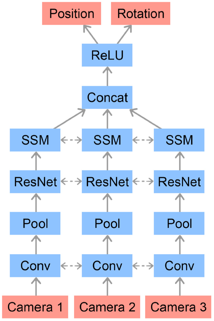
Vision network architecture. Camera images are passed through a convolutional feature stack that consists of two convolutional layers, max-pooling, 4 ResNet blocks (He et al., 2016), and spatial softmax (SSM) (Finn et al., 2015) layers with shared weights between the feature stacks for each camera. The resulting representations are flattened, concatenated, and fed to a fully connected network. All layers use ReLU (Nair and Hinton, 2010) activation function. Linear outputs from the last layer form the estimates of the position and orientation of the object.
Hyperparameters for the vision model architecture.
6.2. Training
We run the trained policy in the simulator until we gather one million states. We then train the vision network by minimizing the mean squared error between the normalized prediction and the ground-truth with minibatch gradient descent. For each minibatch, we render the images with randomized appearance before feeding them to the network. Moreover, we augment the data by modifying the object pose. More specifically, we leave the object pose as is with 20% probability, rotate the object by
Hyperparameters used for the vision model training.
We use NVIDIA P40 GPUs for vision training. Two GPUs are used for rendering and one for the optimization.
7. Results
In this section, we evaluate the proposed system. We start by deploying the system on the physical robot, and evaluating its performance on in-hand manipulation of a block and an octagonal prism. We then focus on individual aspects of our system: we conducted an ablation study of the importance of randomizations and policies with memory capabilities in order to successfully transfer. Next, we consider the sample complexity of our proposed method. Finally, we investigate the performance of the proposed vision pose estimator and show that using only synthetic images is sufficient to achieve good performance.
7.1. Qualitative results
During deployment on the robot as well as in simulation, we note that our policies naturally exhibit many of the grasps found in humans (see Figure 10). Furthermore, the policy also naturally discovers many strategies for dexterous in-hand manipulation described by the robotics community (Ma and Dollar, 2011) such as finger pivoting, finger gaiting, multi-finger coordination, the controlled use of gravity, and coordinated application of translational and torsional forces to the object. It is important to note that we did not incentivize this directly: we do not use any human demonstrations and do not encode any prior into the reward function.
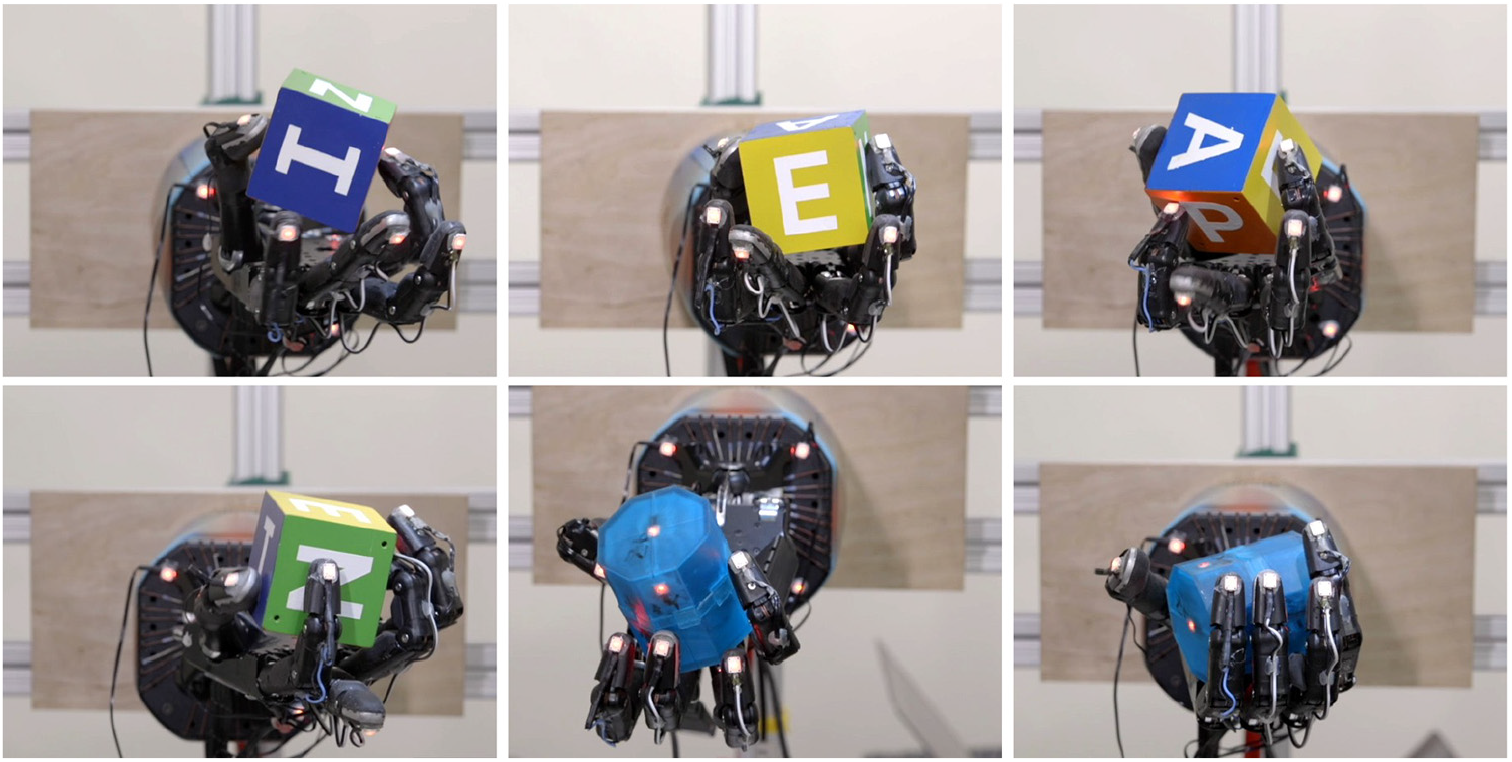
Different grasp types learned by our policy. From top left to bottom right: Tip Pinch grasp, Palmar Pinch grasp, Tripod grasp, Quadpod grasp, 5-Finger Precision grasp, and a Power grasp. Classified according to Feix et al. (2016).
For precision grasps, our policy tends to use the little finger instead of the index or middle finger. This may be because the little finger of the Shadow Dexterous Hand has an extra DoF compared with the index, middle, and ring fingers, making it more dexterous. In humans, the index and middle finger are typically more dexterous. This means that our system can rediscover grasps found in humans, but adapt them to better fit the limitations and abilities of its own body.
We observe another interesting parallel between humans and our policy in finger pivoting, which is a strategy in which an object is held between two fingers and rotate around this axis. It was found that young children have not yet fully developed their motor skills and therefore tend to rotate objects using the proximal or middle phalanges of a finger (Pehoski et al., 1997). Only later in their lives do they switch to primarily using the distal phalanx, which is the dominant strategy found in adults. It is interesting that our policy also typically relies on the distal phalanx for finger pivoting.
During experiments on the physical robot we noticed that the most common failure mode was dropping the object while rotating the wrist pitch joint down. Moreover, the vertical joint was the most common source of robot breakages, probably because it handles the biggest load. Given these difficulties, we also trained a policy with the wrist pitch joint locked. 3 We noticed that not only does this policy transfer better to the physical robot but it also seems to handle the object much more deliberately with many of the above grasps emerging frequently in this setting.
Other failure modes that we observed were dropping the object shortly after the start of a trial (which may be explained by incorrectly identifying some aspect of the environment) and getting stuck because the edge of an object got caught in a screw hole (which we do not model).
We encourage the reader to watch the accompanying video to get a better sense of the learned behaviors (please refer to the supplement material).
7.2. Quantitative results
In this section, we evaluate our results quantitatively. To do so, we measure the number of consecutive successful rotations until the object is either dropped, a goal has not been achieved within 80 seconds, or until
The number of successful consecutive rotations in simulation and on the physical robot. All policies were trained on environments with all randomizations enabled. We performed 100 trials in simulation and 10 trails per policy on the physical robot. Each trial terminates when the object is dropped, 50 rotations are achieved or a timeout is reached. For physical trials, results were taken at different times on the physical robot.
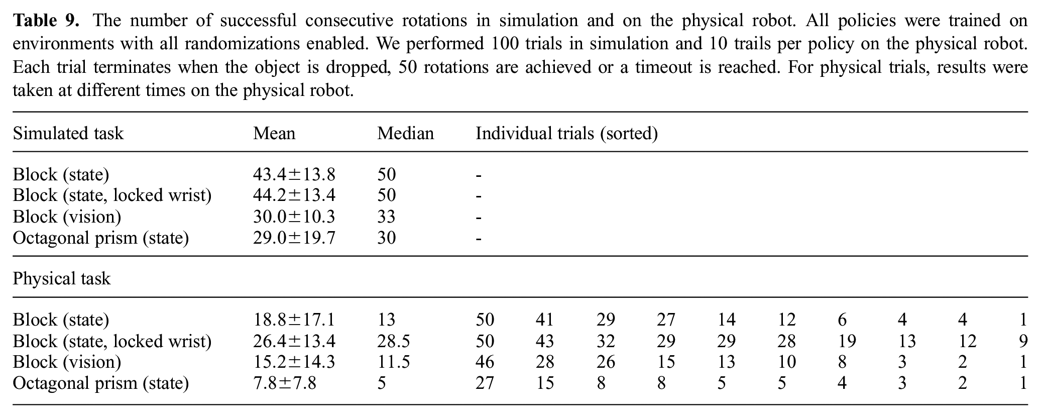
Our results allow us to directly compare the performance of each task in simulation and on the real robot. For instance, manipulating a block in simulation achieves a median of
When using vision for pose estimation, we achieve slightly worse results both in simulation and on the real robot. This is because even in simulation, our model has to perform transfer because it was only trained on images rendered with Unity but we use MuJoCo rendering for evaluation in simulation (thus making this a sim-to-sim transfer problem). On the real robot, our vision model does slightly worse compared with pose estimation with PhaseSpace. However, the difference is surprisingly small, suggesting that training the vision model only in simulation is enough to achieve good performance on the real robot. For vision pose estimation, we found that it helps to use a white background and to wipe the object with a tack cloth between trials to remove detritus from the robot hand.
We also evaluate the performance on a second type of object, an octagonal prism. To do so, we finetuned a trained block rotation control policy to the same randomized distribution of environments but with the octagonal prism as the target object instead of the block. Even though our randomizations were all originally designed for the block, we were able to learn successful policies that transfer. Compared with the block, however, there is still a performance gap both in simulation and on the real robot. This suggests that further tuning is necessary and that the introduction of additional randomization could improve transfer to the physical system.
We also briefly experimented with a sphere but failed to achieve more than a few rotations in a row, perhaps because we did not randomize any MuJoCo parameters related to rolling behavior or because rolling objects are much more sensitive to unmodeled imperfections in the hand such as screw holes. It would also be interesting to train a unified policy that can handle multiple objects, but we leave this for future work.
Obtaining the results in Table 9 proved to be challenging due to robot breakages during experiments. Repairing the robot takes time and often changes some aspects of the system, which is why the results were obtained at different times. In general, we found that problems with hardware breakage were one of the key challenges we had to overcome in this work.
7.3. Ablation of randomizations
In Section 4.2 we detail a list of parameters we randomize and effects we add that are not already modeled in the simulator. In this section, we show that these additions to the simulator are vital for transfer. We train five separate RL policies in environments with various randomizations held out: all randomizations (baseline), no observation noise, no unmodeled effects, no physics randomizations, and no randomizations (basic simulator, i.e., no domain randomization).
Adding randomizations or effects to the simulation does not come without cost; in Figure 11 we show the training performance in simulation for each environment plotted over wall-clock time. Policies trained in environments with a more difficult set of randomizations, e.g., all randomizations and no observation noise, converge much slower and therefore require more compute and simulated experience to train in. However, when deploying these policies on the real robot we find that training with randomizations is critical for transfer. Table 10 summarizes our results. Specifically, we find that training with all randomizations leads to a median of
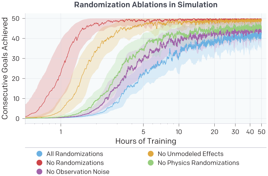
Performance when training in environments with groups of randomizations held out. All runs show exponential moving averaged performance and 90% confidence interval over a moving window of the RL agent in the environment it was trained. We see that training is faster in environments that are easier, e.g., no randomizations and no unmodeled effects. We only show one seed per experiment; however, in general we have noticed almost no instability in training.
The number of successful consecutive rotations on the physical robot of five policies trained separately in environments with different randomizations held out. The first five rows use PhaseSpace for object pose estimation and were run on the same robot at the same time. Trials for each row were interleaved in case the state of the robot changed during the trials. The last two rows were measured at a different time from the first five and used the vision model to estimate the object pose.
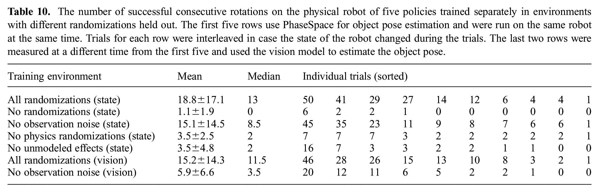
When holding out observation noise randomizations, the performance gap is less clear than for the other randomization groups. We believe that is because our motion capture system has very little noise. However, we still include this randomization because it is important when the vision and control policies are composed. In this case, the pose estimate of the object is much more noisy, and, therefore, training with observation noise should be more important. The results in Table 10 suggest that this is indeed the case, with a drop from median performance of
The vast majority of training time is spent making the policy robust to different physical dynamics. Learning to rotate an object in simulation without randomizations requires about 3 years of simulated experience, while achieving the same performance in a fully randomized simulation requires about 100 years of experience. This corresponds to a wall-clock time of around 1.5 hours and 50 hours in our simulation setup, respectively.
7.4. Effect of memory in policies
We find that using memory is helpful to achieve good performance in the randomized simulation. In Figure 12 we show the simulation performance of three different RL architectures: the baseline which has a LSTM policy and value function, a feed-forward (FF) policy and a LSTM value function, and both a FF policy and FF value function. We include results for a FF policy with LSTM value function because it was plausible that having a more expressive value function would accelerate training, allowing the policy to act robustly without memory once it converged. However, we see that the baseline outperforms both variants, indicating that it is beneficial to have some amount of memory in the actual policy.
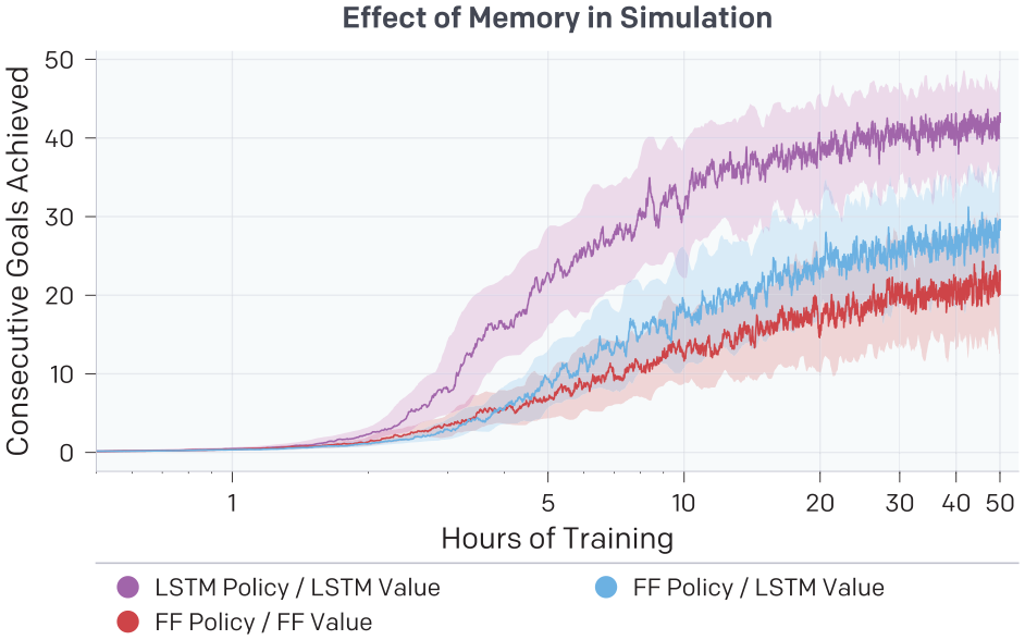
Performance when comparing LSTM and FF policy and value function networks. We train on an environment with all randomizations enabled. All runs show exponential moving averaged performance and 90% confidence interval over a moving window for a single seed. We find that using recurrence in both the policy and value function helps to achieve good performance in simulation.
Moreover, we found out that LSTM state is predictive of the environment randomizations. In particular, we discovered that the LSTM hidden state after 5 seconds of simulated interaction with the block allows to predict whether the block is bigger or smaller than average in 80% of cases.
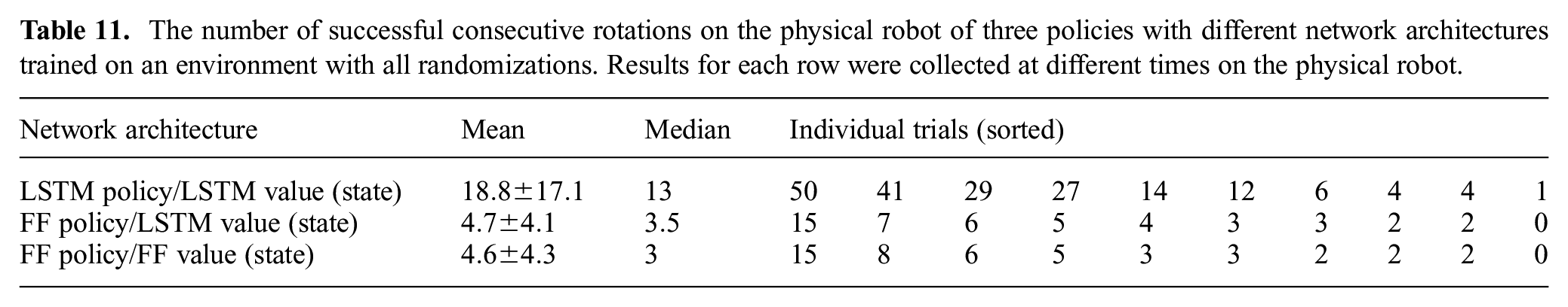
To investigate the importance of memory-augmented policies for transfer, we evaluate the same three network architectures as described above on the physical robot. Table 11 summarizes the results. Our results show that having a policy with access to memory yields a higher median of successful rotations, suggesting that the policy may use memory to adapt to the current environment. 4 Qualitatively we also find that FF policies often get stuck and then run out of time.
The number of successful consecutive rotations on the physical robot of three policies with different network architectures trained on an environment with all randomizations. Results for each row were collected at different times on the physical robot.
In Figure 13 we show results when varying the number of CPU cores and GPUs used in training, where we keep the batch size per GPU fixed such that overall batch size is directly proportional to number of GPUs. Because we could linearly slow down training by simply using less CPU machines and having the GPUs wait longer for data, it is more informative to vary the batch size. We see that our default setup with an 8 GPU optimizer and 6,144 rollout CPU cores reaches 20 consecutive achieved goals approximately 5.5 times faster than a setup with a 1 GPU optimizer and 768 rollout cores. Furthermore, when using 16 GPUs we reach 40 consecutive achieved goals roughly 1.8 times faster than when using the default 8 GPU setup. Scaling up further results in diminishing returns, but it seems that scaling up to 16 GPUs and 12,288 CPU cores gives close to linear speedup.
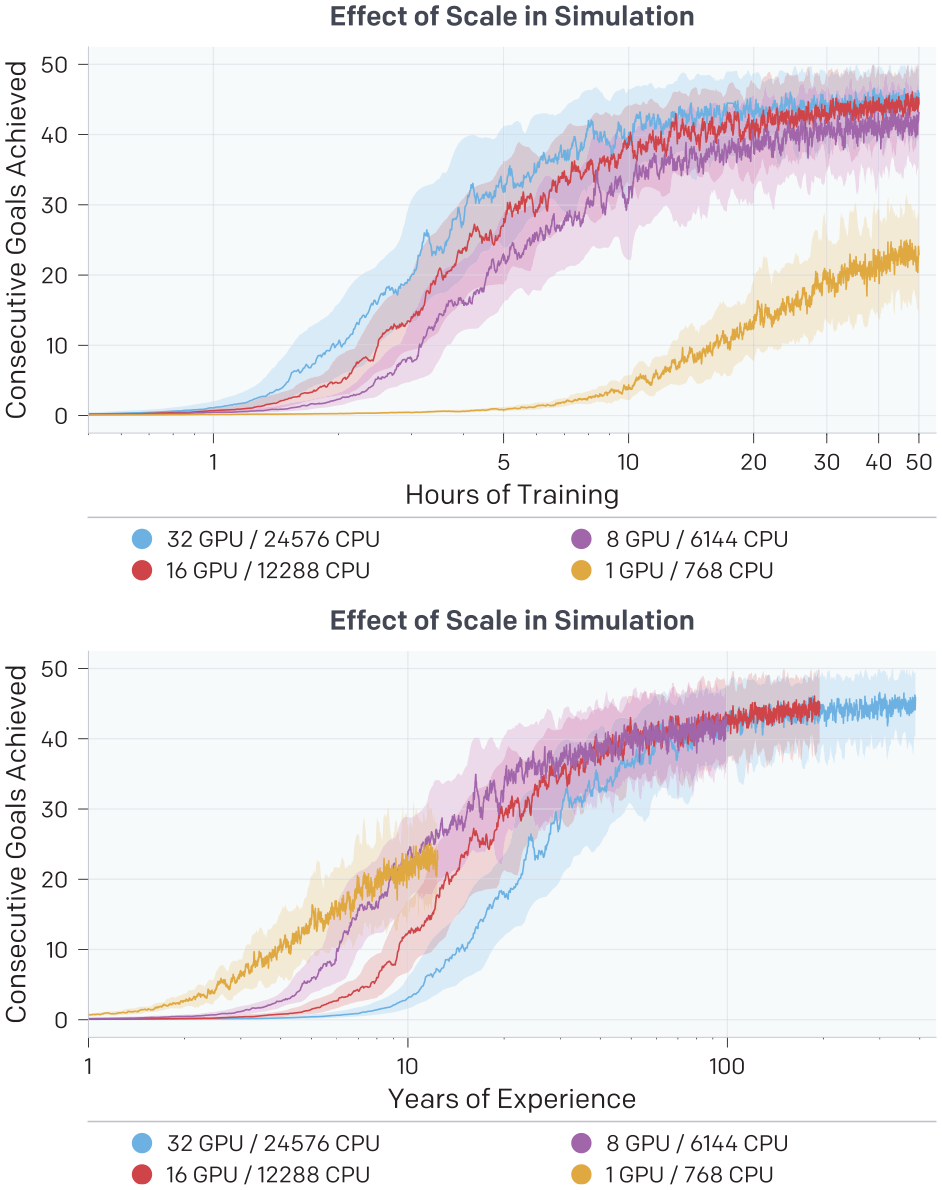
We show performance in simulation when varying the amount of compute used during training versus wall-clock training time (top) and years of experience consumed (bottom). Batch size used is proportional to the number of GPUs used, such that time per optimization step should remain constant apart from slow downs due to gradient syncing across optimizer machines.
7.5. Vision performance
In Table 9 we show that we can combine a vision-based pose estimator and the control policy to successfully transfer to the real robot without embedding sensors in the target object. To better understand why this is possible, we evaluate the precision of the pose estimator on both synthetic and real data. Evaluating the system in simulation is easy because we can generate the necessary data and have access to the precise object’s pose to compare against. In contrast, real images had to be collected by running a state-based policy on our robot platform. We use PhaseSpace to estimate the object’s pose, which is therefore subject to errors. The resulting collected test set consists of
Performance of a vision based pose estimator on synthetic and real data.
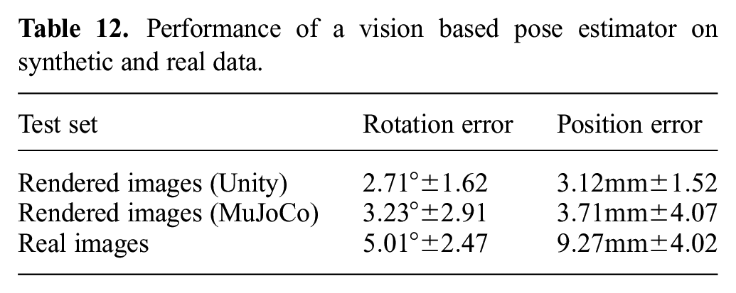
Our results show that the model achieves low error for both rotation and position prediction when tested on synthetic data. 6 On the images rendered with MuJoCo, there is only a slight increase in error, suggesting successful sim-to-sim transfer. The error further increases on the real data, which is due to the gap between simulation and reality but also because the ground truth is more challenging to obtain due to noise, occlusions, imperfect marker placement, and delayed sensor readings. Despite that the prediction error is bigger than the observation noise used during policy training (Table 1), the vision-based policy performs well on the physical robot (Table 9).
8. Related work
In order to make it easier to understand the state of the art in dexterous in-hand manipulation we gathered a representative set of videos from related work, and created a playlist out of them (see the supplemental material).
8.1. Dexterous manipulation
Dexterous manipulation has been an active area of research for decades (Bicchi, 2000; Fearing, 1986; Ma and Dollar, 2011; Okamura et al., 2000; Rus, 1999). Many different approaches and strategies have been proposed over the years. This includes rolling (Bicchi and Sorrentino, 1995; Cherif and Gupta, 1999; Doulgeri and Droukas, 2013; Han et al., 1997; Han and Trinkle, 1998), sliding (Cherif and Gupta, 1999; Shi et al., 2017), finger gaiting (Han and Trinkle, 1998), finger tracking (Rus, 1992), pushing (Dafle and Rodriguez, 2017), and re-grasping (Dafle et al., 2014; Tournassoud et al., 1987). For some hand types, strategies such as pivoting (Aiyama et al., 1993), tilting (Erdmann and Mason, 1988), tumbling (Sawasaki and Inoue, 1991), tapping (Huang and Mason, 2000), two-point manipulation (Abell and Erdmann, 1995), and two-palm manipulation (Erdmann, 1998) are also options. These approaches use planning and therefore require exact models of both the hand and object. After computing a trajectory, the plan is typically executed open-loop, thus making these methods prone to failure if the model is not accurate. 7
Other approaches take a closed-loop approach to dexterous manipulation and incorporate sensor feedback during execution, e.g., tactile sensing (Li et al., 2014a,b, 2013; Tahara et al., 2010). While those approaches allow mistakes to be corrected at runtime, they still require reasonable models of the robot kinematics and dynamics, which can be challenging to obtain for under-actuated hands with many DoFs.
Deep RL has also been used successfully to learn complex manipulation skills on physical robots. Guided policy search (Levine and Koltun, 2013; Levine et al., 2015) learns simple local policies directly on the robot and distills them into a global policy represented by a neural network. An alternative is to use many physical robots simultaneously in order to be able to collect sufficient experience (Gu et al., 2017; Kalashnikov et al., 2018; Levine et al., 2018).
8.2. Dexterous in-hand manipulation
Since a very large body of past work on dexterous manipulation exists, we limit the more detailed discussion to setups that are most closely related to our work on dexterous in-hand manipulation.
Mordatch et al. (2012) and Bai and Liu (2014) proposed methods to generate trajectories for complex and dynamic in-hand manipulation, but results were limited to simulation. There has also been significant progress in learning complex in-hand dexterous manipulation (Barth-Maron et al., 2018; Plappert et al., 2018) and even tool use (Rajeswaran et al., 2017) using deep RL, but those approaches were also only evaluated in simulation.
In contrast, multiple authors learn policies for dexterous in-hand manipulation directly on the robot. van Hoof et al. (2015) learned in-hand manipulation for a simple three-fingered gripper whereas Kumar et al. (2016a,b) and Falco et al. (2018) learned such policies for more complex humanoid hands. While learning directly on the robot means that modeling the system is not an issue, it also means that learning has to be performed with only a handful of trials. This is only possible when learning very simple (e.g., linear or local) policies that, in turn, do not exhibit sophisticated behaviors.
8.3. Sim-to-real transfer
Domain adaption methods (Gupta et al., 2017; Tzeng et al., 2015), progressive nets (Rusu et al., 2017), and learning inverse dynamics models (Christiano et al., 2016) were all proposed to help with sim-to-real transfer. All of these methods assume access to real data. An alternative approach is to make the policy itself more adaptive during training in simulation using domain randomization. Domain randomization was used to transfer object pose estimators (Tobin et al., 2017a) and vision policies for fly drones (Sadeghi and Levine, 2017). This idea has also been extended to dynamics randomization (Antonova et al., 2017; Tan et al., 2018; Yu et al., 2017) to learn a robust policy that transfers to similar environments but with different dynamics. Domain randomization was also used to plan robust grasps (Mahler et al., 2017a,b; Tobin et al., 2017b) and to transfer learned locomotion (Tan et al., 2018) and grasping (Zhu et al., 2018) policies for relatively simple robots. Pinto et al. (2017b,c) proposed the use of adversarial training to obtain more robust policies and showed that it also helps with transfer to physical robots.
9. Conclusion
In this work, we have demonstrated that in-hand manipulation skills learned with RL in a simulator can achieve an unprecedented level of dexterity on a physical five-fingered hand. This is possible due to extensive randomizations of the simulator, large-scale distributed training infrastructure, policies with memory, and a choice of sensing modalities that can be modeled in the simulator. Our results have demonstrated that, contrary to a common belief, contemporary deep RL algorithms can be applied to solving complex real-world robotics problems that are beyond the reach of existing non-learning-based approaches.
Footnotes
Acknowledgements
We would like to thank Rachel Fong, Ankur Handa, and a former OpenAI employee for exploratory work and helpful discussions, a former OpenAI employee for advice and some repairs on hardware and contributions to the low-level PID controller, Pieter Abbeel for helpful discussions, Gavin Cassidy and Luke Moss for their support in maintaining the Shadow Hand, and everybody at OpenAI for their help and support. We would also like to thank the following people for providing feedback on earlier versions of this manuscript: Pieter Abbeel, Joshua Achiam, Tamim Asfour, Aleksandar Botev, Greg Brockman, Rewon Child, Jack Clark, Marek Cygan, Harri Edwards, Ron Fearing, Ken Goldberg, Anna Goldie, Edward Mehr, Azalia Mirhoseini, Lerrel Pinto, Aditya Ramesh, Ian Rust, John Schulman, Shubho Sengupta, and Ilya Sutskever.
Funding
This research received no specific grant from any funding agency in the public, commercial, or not-for-profit sectors.