
Abstract
Concentric tube robots offer the capability of follow-the-leader motion, which is desirable when navigating in cluttered environments, such as in minimally invasive surgery or in-situ inspections. The follow-the-leader capabilities identified in the existing literature, however, are limited to trajectories with piecewise constant-curvature segments or piecewise helical segments. A complete study of follow-the-leader kinematics is, therefore, relevant to determine the full potential of these robots, and clarify an open question. In this paper, a general analysis of follow-the-leader motion is presented, and a closed-form solution to the complete set of trajectories where follow-the-leader is possible under the assumption of no axial torsion of the tubes composing the robot is derived. For designs with constant-stiffness tubes, the precurvatures required are found to be either circumference arcs, helices, or deformed helices with exponentially varying curvature magnitude. The analysis developed also elucidates additional motions of interest, such as the combination of follow-the-leader motion in a robot segment with general maneuvers in another part. To determine the applicability of the assumption regarding the tubes’ torsion, the general equilibrium of the robot designs of interest is considered, and a closed-form solution to torsion in two-tube robots with helical precurvatures is derived. Criteria to select a desired torsional behavior are then extracted. This enables one to identify stable trajectories where follow-the-leader is possible, for potential application to minimally invasive surgery. An illustrative case study involving simulation and experiment is conceived using one of these trajectories, and the results are reported, showcasing the research.
1. Introduction
Concentric tube robots were originally proposed a decade ago by Sears and Dupont (2006) and Webster et al. (2006), and since then their popularity has been increasing, predominantly in the field of minimally invasive surgery. The rapid uptake of these robots can be credited to the advantages they offer when operating in confined environments. These advantages include a small diameter similar to that of a surgical needle, a simple mechanical design requiring a small number of parts, and singular kinematics that provide the ability to advance in follow-the-leader motion, i.e. the robot structure follows the path selected by its distal end, in specific trajectories.
A concentric tube robot consists of a set of precurved, super-elastic tubes arranged concentrically. The geometry of the robot is therefore determined by the elastic equilibrium of the tubes that compose it. The control of the relative insertion and rotation of the tubes enables control of the robot’s motion. It should be noted, however, that the motion achievable by a specific robot depends on its design in terms of the precurvature and stiffness of the tubes that comprise it.
Research on the different aspects of concentric tube robots is reported in the literature. The mechanical analysis of these robots is well established, with traditional approaches assuming no external loads and no friction, such as in Dupont et al. (2009) and Webster et al. (2009), and subsequent studies considering external forces, as in Mahvash and Dupont (2011) and Rucker et al. (2010), and also including friction between tubes (Lock and Dupont, 2011). As a result, accurate control of the robots is possible (Dupont et al., 2010a,b), and stable paths can be planned (Bergeles and Dupont, 2013; Lyons et al., 2009, 2010). In addition,feedback systems based on fiber Bragg gratings have been proposed and incorporated into the robots (Ryu and Dupont, 2014), enabling closed-loop control with proprioceptive sensing.
All this established research has allowed applications in a range of medical procedures, including Burgner et al. (2011); Butler et al. (2012); Dupont et al. (2012); Gosline et al. (2012); Vasilyev et al. (2013), which showcase the capabilities of concentric tube robots. Current work, however, is focused on the exploitation of robot designs composed of piecewise constant-curvature tubes. A first study of other trajectories traceable in a follow-the-leader configuration was recently published by Gilbert et al. (2015). However, this work only offers solutions for some specific robot configurations, but it does not allow a general study, leaving general follow-the-leader possibilities as an open question. A general study is therefore required to determine the complete follow-the-leader possibilities that concentric tube robots can offer, based on existing models, thereby establishing the full potential of these devices.
In this paper, the full follow-the-leader capabilities achievable with concentric tube robots are analyzed, and a closed-form solution to the complete set of trajectories that can be followed in a follow-the-leader configuration under the assumption of no axial torsion of the tubes is presented. The validity of such an assumption is subsequently considered in the set of trajectories discovered, which allows for the selection of a case study to showcase the work. The objective of this work is similar to that in Gilbert et al. (2015), and therefore some parallels are present, as noted throughout this paper. However, the research presented here was conducted independently of Gilbert et al. (2015), which favored the formulation of a different approach that enables a general study and solution. This clarifies a currently open question, and broadens the potential of concentric tube_ robots with a new set of trajectories that can be exploited in, for instance, minimally invasive surgery or in-situ inspections. A crucial part of the approach adopted here is a specific robot description, which allows a geometrical interpretation of the conditions for follow-the-leader motion. This enables the formulation of a treatable problem and the derivation of a general, closed-form solution under the assumption of no axial torsion of the tubes.
The formulation of the analysis presented in this work considers robots comprising any number of tubes with any desired precurvature and stiffness, and any possible control strategy in terms of rotation and insertion of the tubes. Discontinuities in robot curvature, which are inherent in telescopic robot deployment as well as in unconventional robot designs, are also considered in the study. Thus, the analysis of follow-the-leader motion reported here, together with the corresponding solutions, is completely general. In addition, the geometrical interpretation of follow-the-leader motion proposed in this paper provides conceptual insight into these kinematics, which is useful for the future development of path planning and closed-loop control algorithms, and for the application of these robots to practical scenarios, where disturbances are present.
The strategy employed in this work to study the follow-the-leader possibilities, which involves first studying the problem assuming no torsion and then determining the validity of the assumption, is advantageous from both a theoretical and practical perspective. It establishes the full capabilities first under the assumption of no torsion, and then it enables selection of the admissible deviation in terms of torsion of the tubes. In this manner, useful trajectories with a small deviation away from an ideal follow-the-leader configuration are not discarded, which can be advantageous. Furthermore, since the admissible deviation in terms of torsion can be selected, it can be specified to be as close to zero as desired. Still, the design of concentric tube robots accepting a relatively small deviation from follow-the-leader due to torsion is advisable, considering that it noticeably increases the number of feasible trajectories, and that, in practice, a certain degree of uncertainty generally exists in the predicted robot behavior. It should be noted that the focus here is on the deviation in terms of local curvature from that corresponding to follow-the-leader motion, but this does not directly imply a specific deviation in task space. The relation between deviation in task space and local deviation due to torsion is illustrated with some simulations of relevant configurations, but the determination of the specific relation is a question beyond the scope of this present work. Interestingly, the analysis assuming no torsion is also applicable to robot designs with non-annular cross-sections, originally proposed in Greenblatt et al. (2011), by simply considering controls without relative rotation of the tubes.
To study the torsion of tubes and then conceive a case study to showcase this research, the general equilibrium of the robot is considered in the set of trajectories discovered. A closed-form solution describing the torsion of the tubes along the arc length is obtained for two-tube robots with helical precurvatures, which represent the most relevant designs in the trajectories discovered. This solution then allows for identification of the designs that guarantee that the torsion of the tubes is below a specified value. Interestingly, the torsional behavior is found to depend on two non-dimensional groups, which indicate that torsional deviation can be reduced by using helical tubes the precurvatures of which have significantly different geometric torsion. These results are used to develop a case study involving simulation and experiment, where the tubes present a small torsional deformation and the robot maintains a near perfect follow-the-leader configuration, illustrating the capabilities described in this work.
The set of trajectories found in this work is non-trivial, and expands the currently known capabilities of concentric tube robots. For robots composed of constant-stiffness tubes, the corresponding robot designs required are found to be composed of tubes with precurvatures that are either helices or deformed helices with exponentially varying curvature magnitude. For robots with variable stiffness tubes, robot designs composed of tubes with more general geometries associated with the deformation of helices are found to be possible. It should be noted that the idea of considering helical precurvatures for follow-the-leader motion has been previously proposed by Gilbert et al. (2015), but in this work it is extended and formalized. Kinematic equivalences that can be exploited within the follow-the-leader set of trajectories are also extracted from the analysis. These include concatenation of segments of different trajectories, or the addition of idle tubes that become active once inserted. Furthermore, various maneuvers that combine follow-the-leader motion along a segment of the concentric tube robot with general displacements at its distal end, which do not correspond to follow-the-leader, are also distilled from the analysis. These maneuvers are aimed at applications where the robot end-effector is able work in a spacious cavity, which can only be accessed through a narrow path that requires follow-the-leader motion. Such a situation is common in minimally invasive surgery, as well as in other fields, such as in-situ inspections, where the kinematics identified here can offer a significant advantage. It should be noted that the majority of these kinematic possibilities have already been proposed in the literature for robot designs composed of piecewise constant-curvature tubes (e.g. Dupont et al., 2010b, 2012; Gosline et al., 2012). In this work, these are generalized and integrated into the analysis developed here.
The paper is structured as follows. The governing equations of a general concentric tube robot under the assumption of no axial torsion are derived in Section 2. The study of follow-the-leader motion is presented Section 3, where the closed-form solution corresponding to the trajectories traceable in a follow-the-leader configuration is derived. In Section 4, additional maneuvers of interest that can be deduced from the analysis of follow-the-leader motion are described. The structural analysis considering torsion of the tubes composing a robot is outlined in Section 5, including the closed-form solution to the tubes’ torsion in a two-tube configuration. Finally, the case study involving simulation and experiment is presented in Section 6, together with the corresponding results, which leads to the conclusion of the paper in Section 7.
2. Governing equations
The relations that govern the behavior of the robotic system are derived in this section. The analysis follows a similar approach to that in the established literature, and Dupont et al. (2010b) is used as the main reference throughout the paper to facilitate the reading. However, some variations on the analysis are introduced in order to adapt it to the aims of this work, with associated changes in nomenclature.
2.1. Problem characterization
The problem description adopted in this work is crucial to enable derivation of the solutions presented in the following sections. In this regard, a detailed characterization of the problem is presented in this subsection. The geometry of a tube, or a set of concentric tubes, is described by the curve corresponding to its centerline. Diameter variations are not expected, nor relevant to this study, and only the cross-sectional moment of inertia is necessary, as elucidated in the following subsection. Vectors, and in particular curvature, are expressed using Bishop reference frames (Bishop, 1975). In particular, a frame W is defined as a Bishop frame corresponding to the final robot geometry, as initially proposed by Sears and Dupont (2006), and a frame
The following magnitudes are then used to characterize a concentric tube robot. The length of the relevant part of the robot, which generally corresponds to the inserted robot length, is denoted L. The position along the arc length is represented by s, relative to the distal end and defined positive
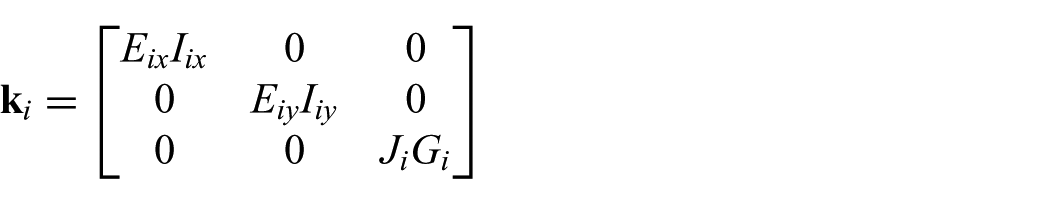
where E is the Young modulus and
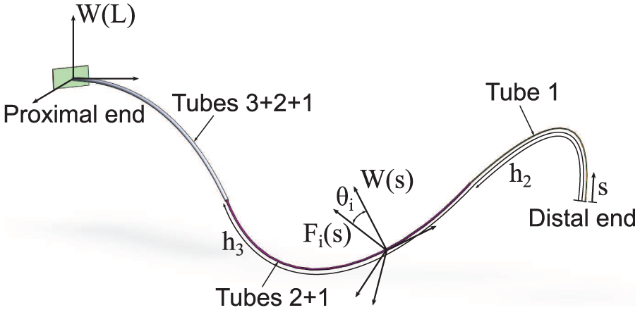
General concentric tube robot composed of three tubes with relevant nomenclature definitions.
From this problem description, the advantages of using Bishop frames (Bishop, 1975) are clear. First, Bishop frames are intrinsic reference frames with one component always parallel to the curve tangent vector, which is convenient, considering that the vector curvature is orthogonal to the tube’s centerline curve. In addition, they are defined in any curve that is sufficiently differentiable, even at points with zero curvature. Finally, for a tube with no axial torsion, the curvature along the tube can be transformed to another Bishop frame with a simple rotation that is constant along the entire tube.
2.2. Governing laws
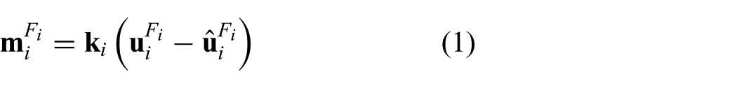
The behavior of the robotic system is governed by three laws. First, an elastic constitutive law, which can be obtained following Dupont et al. (2010b) as
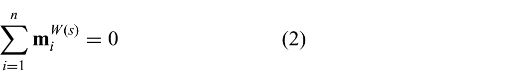
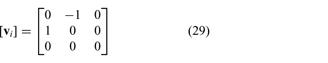
Second, a static equilibrium law (assuming a quasistatic operation of the robot), which can be written as
Finally, a law preventing the superposition of matter (using a continuum mechanics description of matter), which translates into a condition that imposes a common final curvature to the tubes that compose a robot when arranged concentrically
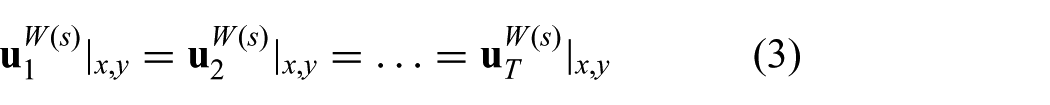
which only applies to the x,y components of
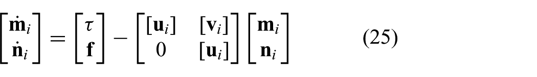
Assuming no external loads, and no axial torsion of the tubes, combination of all three laws (equations (1), (2), and (3)) determines the robot quasistatic model
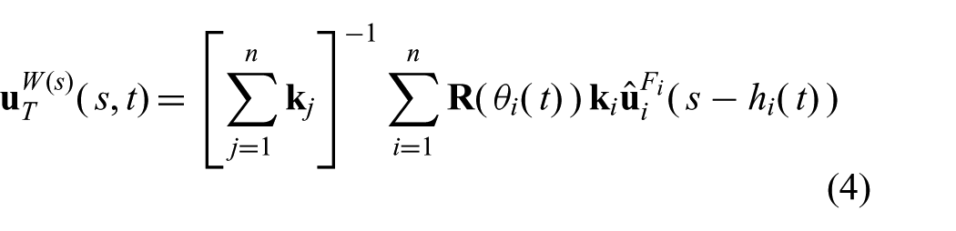
where
expressed in a Bishop frame corresponding to the final robot curvature with no axial torsion. The orientation of this final Bishop frame around the z axis is defined by a desired arbitrary frame in a given cross-section, e.g. the proximal end of the robot, and the corresponding extension to the entire curve of the robot centerline. As a consequence, rigid body rotations of the robot are represented by a simple rotation of all tubes with a common angular velocity. It should be noted that the composition
Equation (4) elucidates the fact that both the tubes and the robot’s final curvature can be expressed using a vector with only two components. However, in order to be consistent with literature, and to clarify the use of the assumption of no axial torsion, a three-dimensional vector is employed.
3. Follow-the-leader
Equation (4) describes all possible geometries that a concentric tube robot with design parameters
In this section, the robot kinematics corresponding to id="math7-the-leader motion are studied. The condition for follow-the-leader motion is first elucidated in Subsection 3.1. This condition is then imposed on the quasistatic model of a general concentric tube robot in Subsection 3.2, yielding the vectorial equation that must be satisfied for a trajectory to be traceable in follow-the-leader motion. The complete solutions to this equation are then studied in Subsection 3.3, leading to the complete set of trajectories where follow-the-leader is possible in Subsection 3.4. It should be noted that the strategy of defining a kinematic condition for follow-the-leader motion and then imposing it on the robot model is similar to that proposed in Gilbert et al. (2015). However, the specific analysis is markedly different, which is a consequence of the fact that this research was conducted independently. In this regard, the study in this paper is complementary to that of Gilbert et al. (2015), and in this case leads to the solutions derived in the following subsections.
3.1. General condition
Follow-the-leader motion requires the curve corresponding to the robot centerline to remain in a constant spatial curve, except for the differential segment that advances with a differential of t . Thus, the curvature of the robot centerline must be constant for all spatial locations. Defining a magnitude x, which corresponds to spatial location in the workspace, the condition imposing curvature at each spatial location to remain constant can be expressed as

where C is the locus of the curve corresponding to the robot centerline. Considering that the robot curvature can be expressed as a function of s and t, as described in the previous section, the expression of curvature at a spatial location can be differentiated. Since the curvature must be constant at each spatial location, as expressed in equation (5), differentiation yields the condition for follow-the-leader in the robot segments with differentiable curvature as
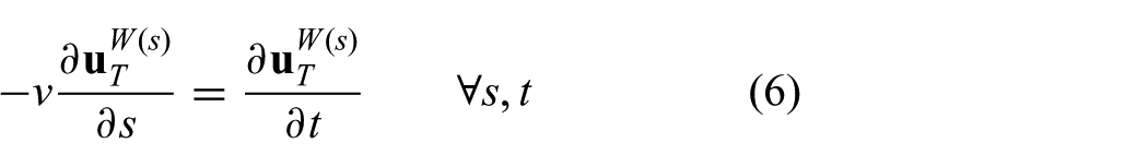
It should be noted that the time-dependent variables in
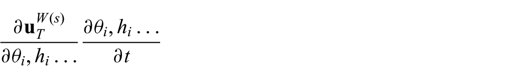
for all i . Equation (6) indicates that, in order to advance in a follow-the-leader configuration, the curvature of each cross-section must pass to the immediate adjacent cross-section toward the proximal end. In a reference frame positioned at the distal end of the robot, this motion resembles that of a wave without attenuation traveling toward the base of the concentric tube robot, as conceptually illustrated in Figure 2.
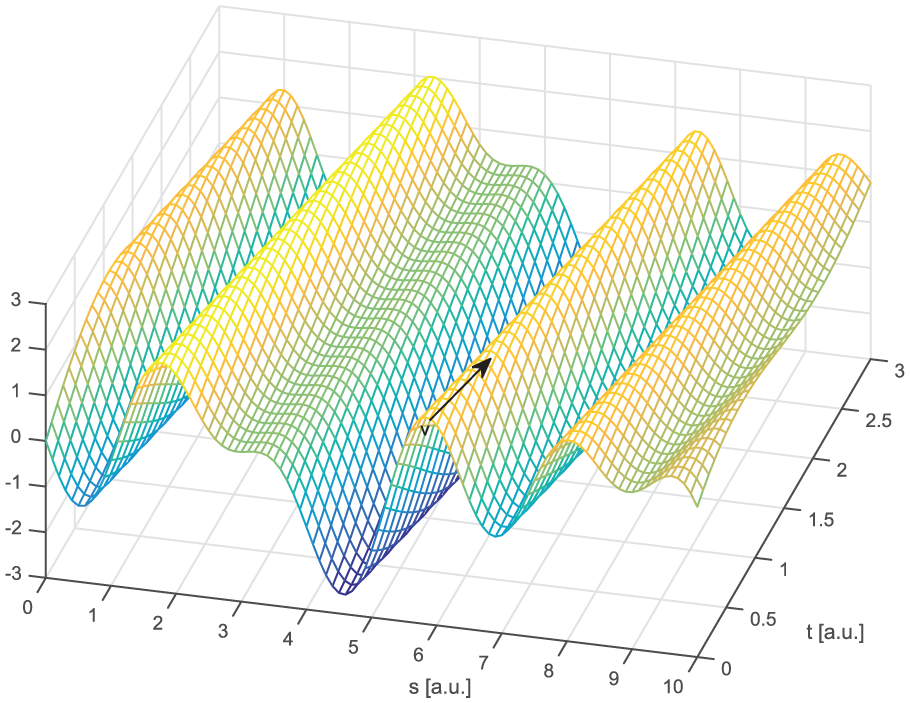
Conceptual illustration of a Curvature field corresponding to follow-the-leader configuration. A vector of motion that satisfies follow-the-leader is indicated with a black arrow.
For robots with continuous
3.2. Application to concentric tube robots
The imposition of equation (6) on the quasistatic model of the robot (equation (4)) restricts the possible robot kinematics to those that correspond to perfect follow-the-leader motion (if any). This yields the condition that suffices for a trajectory to be traceable by a concentric tube robot in a follow-the-leader configuration
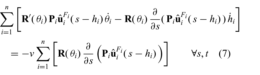
where
and
and both
The curve describing trajectories where follow-the-leader is possible can be specified both by the corresponding
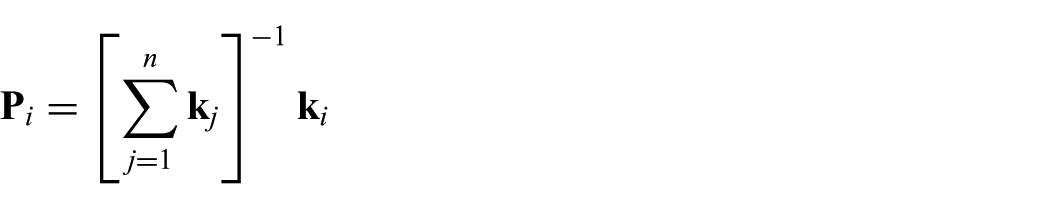
In concentric tube robots,
The complete solution to equation (7) therefore corresponds to the complete set of trajectories where follow-the-leader is possible under the assumption of no axial torsion. It should be noted that equation (7) is applicable to any robot design in terms of precurvatures, stiffness, and number of tubes, for any possible control strategy. Thus, it represents a general condition for follow-the-leader motion.
The problem description employed in this work allows the derivation of a closed-form solution to equation (7). The key to such a solution is to treat equation (7) from a vectorial perspective, rather than decoupling it into a system of individual differential equations. Considering that all terms in equation (7) either contain
3.3. Solution cases
The approach adopted here to study the solution to equation (7) involves dividing the problem into cases of increasing complexity for clarity of exposition, as presented in this subsection. Cases with restrictions on the motions allowed with the tubes are considered first, serving as a foundation for the subsequent study of more general cases.
3.3.1. Rotation only and different for each tube
Considering first a case where the rotation of the tubes is the only input allowed (equal insertion rate of all tubes), and considering that no groups of tubes are moving together, i.e. functions
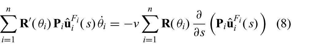
The possible solutions to equation (8) can be divided into two cases: the terms in equation (8) corresponding to each tube compensate so that their sum is null, which will be referred to as “compensating individually”, or the terms in equation (8) from different tubes combine so that their sum is zero, which will be referred to as “compensating in conjunction.”
In the case of compensating individually, equation (8) is particularized as
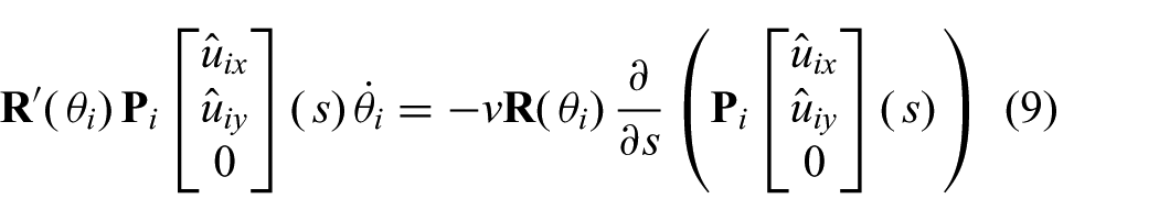
which must be satisfied for all time. The only time-dependent terms are matrices
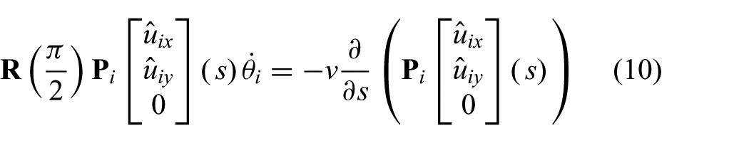
The solution to equation (10) can be easily obtained by realizing that it imposes
Follow-the-leader motion using only relative rotation of the tubes and compensating individually is therefore possible, and the resulting trajectories expressed as the resulting geometry of the robot at the time corresponding to the end of an insertion are
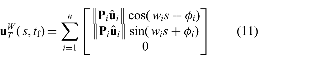
where
In the case of compensating in conjunction, solutions to equation (8) can also be derived in specific configurations. Rewriting equation (8), relying on the fact that
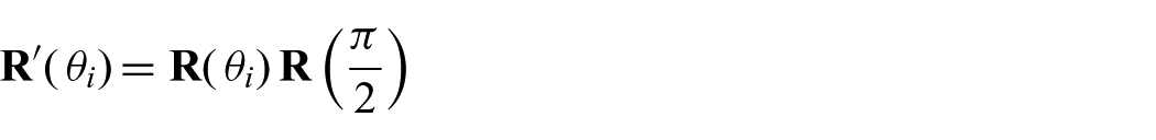
yields
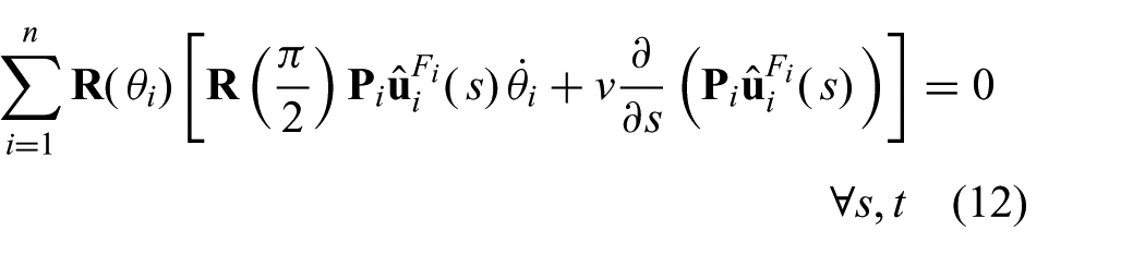
The terms in equation (12) are a sum of planar vectors in each cross-section, and thus vectors
The magnitude of the vectors in equation (12) is either fixed, for
Considering first a case with l=2, two variables
Two possible design solutions then arise: (i)
Considering a general case with l > 2, an equivalent analysis applies, although some specific differences are present. The number of variables
The trajectories that can be traced in a follow-the-leader configuration with robots comprising only a set of tubes i ∈ l that compensate in conjunction must then correspond to a
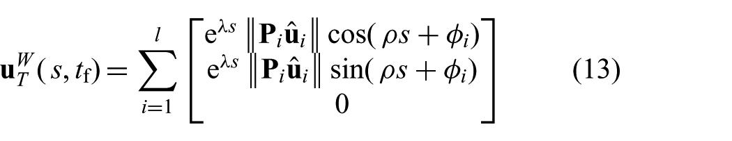
where λ is a parameter corresponding to the increase in curvature magnitude along the arc length, which can be selected with the tubes’ design and is common for tubes i ∈ l, ρ is a parameter corresponding to the geometric torsion of the tubes, also common for tubes i ∈ l, and
where
Compensating in conjunction requires at least two tubes in order to have two inputs
Follow-the-leader motion using only relative rotation of the tubes is thus possible both compensating individually and in conjunction. Equation (8) is a summation of terms corresponding to different tubes. Hence, any combination of solutions corresponding to a set of tubes compensating individually (equation (11)) and a set of tubes compensating in conjunction (equation (14)) must also satisfy equation (8). The resulting set of trajectories is then
where g is the number of sets of tubes that involve compensating in conjunction, and
As a particular solution to equation (15), the trajectory corresponding to a single tube being inserted is a helix relative to the workspace. In this case, the required tube precurvature is equal to the resulting trajectory, a configuration that corresponds to a common device, namely the corkscrew. It should be noted that the helix can be degenerated to a circumference arc, elucidating the fact that this result is completely general.
3.3.2. Different rotation and insertion for each tube
Considering now the case where any independent combination of insertion and rotation of the tubes as a function of time is allowed, but no groups of tubes move together, i.e. functions
In the case of compensating individually, equation (7) particularizes to
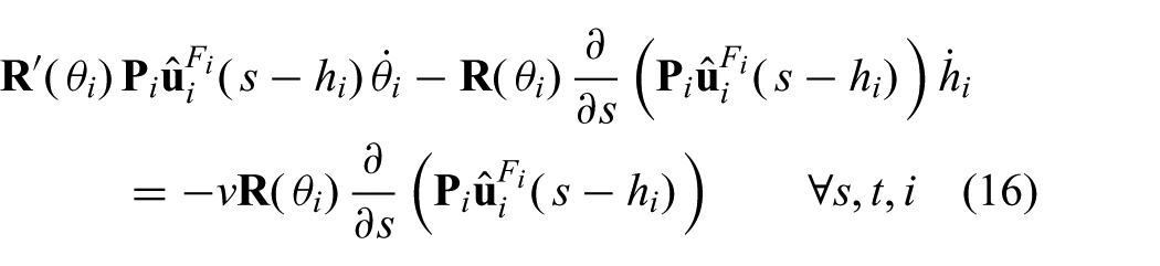
Regrouping, equation (16) can be rewritten as
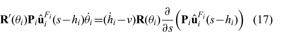
which must also be satisfied for all s,t,i. Equation (17) simplifies the geometrical interpretation of the differential equation, elucidating the relation that must be satisfied between vector
Two different design possibilities in terms of precurvatures and stiffness of the tubes comprising the robot arise from equation (17), which depend on whether the modulus of
If
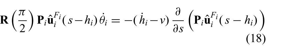
The solution to equation (18) is, as in the previous case, a vector
If
In the case of compensating in conjunction, specific control inputs
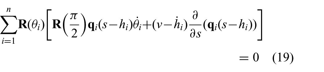
which must hold for all s, t.
Equation (19) is a sum of planar vectors with a relative orientation that varies with t owing to the different
The selection of
Compensating in conjunction involves two or more tubes. Configurations with two tubes lead to a robot with two degrees of freedom, as four inputs (
It should be noted that the trivial solution
The previous discussion for both configurations compensating individually or in conjunction shows that the use of the relative tube’s insertion as control input
In the case of compensating individually, the control input for each tube is also restricted by equation (17). To satisfy equation (17) at a given time instant, a specific tube geometry must be selected, as previously discussed. Once the geometry is specified, equation (17) imposes a constant relation between

where
Equation (20) corresponds to the control input required in each individual tube to satisfy the follow-the-leader condition (equation (17)). Equation (20) elucidates the aforementioned freedom in the follow-the-leader control of each individual tube, where different combinations of
In the case of compensating in conjunction, the required control inputs
The degrees of freedom of the control inputs can be seen in equation (4), where both
The condition for follow-the-leader (equation (7)) is a sum of terms corresponding to different tubes. Therefore, as in Subsection 3.3.1, combinations of configurations that involve compensating individually and compensating in conjunction also satisfy equation (7). The complete set of trajectories that can be traced in a follow-the-leader configuration under the assumptions of this second case is then equal to that in the previous subsection (equation (15)). The only extension in terms of follow-the-leader motion is the possibility of leaving tubes static relative to the workspace while the rest of the robot advances.
3.3.3. General configuration including groups of tubes
Considering now the most general case, where any control inputs are allowed, the solutions to equation (7) are generally equivalent to those in the previous case, with the exception of configurations where groups of tubes move with a common
In the case of each group compensating individually, the terms of each group must then satisfy
where
(i) If
Alternatively, by selecting a specific
(ii) If
which is equivalent to case (ii) of Subsection 3.3.2, so no new trajectories are added.
(iii) If
Alternatively, by selecting specific
In the case of various groups of tubes compensating in conjunction, the groups must satisfy
where
(iv) If
(v) If the
From the discussion in this subsection, it can be concluded that the combination of a group of tubes with a common
3.3.4. Curvature discontinuities
Up to this point, the study of trajectories where follow-the-leader is possible considered only continuous curves satisfying equation (6). However, trajectories with curvature discontinuities can also be traced in a follow-the-leader configuration, provided that the conditions described in Subsection 3.1 are satisfied. An example is the well-established trajectory composed of circumference arcs (Sears and Dupont, 2006).
In general, the points of curvature discontinuity must remain in a constant position in the workspace, which implies that they must translate at velocity v away from the robot’s distal end as it advances. This requires the tubes causing the discontinuity to have
3.4. Set of trajectories summary
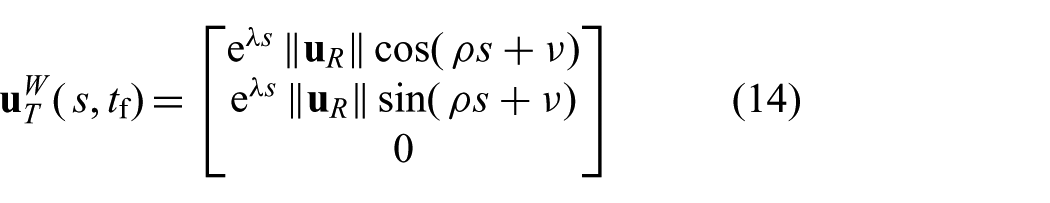
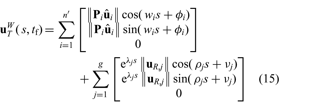
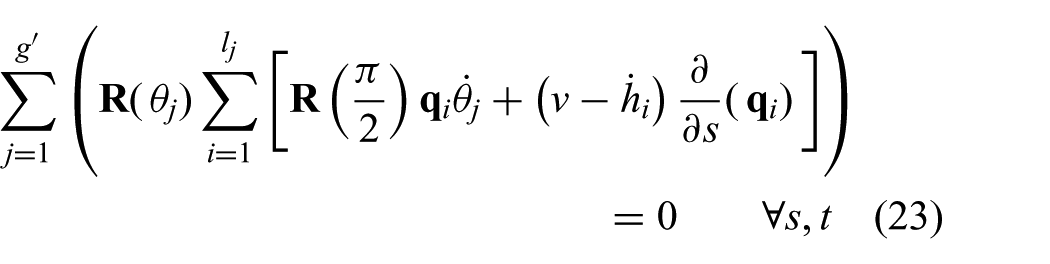
The trajectories found in Subsections 3.3.1 to 3.3.3, together with their combinations in Subsection 3.3.4, constitute the set of trajectories that can be traced in a follow-the-leader configuration, since all possible cases solving equation (7) have been considered, in addition to curvature discontinuities. The trajectories, excluding combinations of them, can be synthesized in a single expression
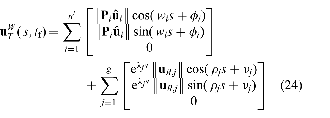
where
The initial designs of the individual tubes or groups of tubes comprising a concentric tube robot capable of follow-the-leader motion must satisfy
The robot designs corresponding to equation (24), however, are not limited to tubes with helical precurvatures. If tubes with variable stiffness are used, the precurvatures can present more general geometries that correspond to the deformation of helices, provided that the aforementioned relations on
It should be noted that
Equation (24), together with combinations of the trajectories linked as introduced in Subsection 3.3.4, represent the complete set of trajectories that can be traced in follow-the-leader motion under the assumption of no axial torsion of the tubes. A broad variety of trajectories can therefore be followed. However, it should be noted that a generic robot design cannot be used to follow any desired trajectory in the set (equation (24)), and instead a robot must be designed to follow a desired, small subset of the trajectories determined by variations in the
The control input required in each tube or group of tubes to maintain follow-the-leader motion over an entire concentric tube robot is given by equation (20) with
The set of trajectories summarized in equation (24) is broad, and torsion can be expected to occur in some of the trajectories. This can render some of the trajectories partially inaccurate or completely unfeasible, as studied in Section 5. Before the analysis of torsion, additional kinematics of interest are considered in the following section, completing the general study of motion related to follow-the-leader.
4. Additional maneuvers
The kinematic analysis presented up to this point focused on follow-the-leader motion. However, some potentially exploitable kinematic possibilities were also found in the discussion. The applicability of these kinematics, together with additional motions related to follow-the-leader motion, are described in this section. The majority of these kinematics have been previously proposed in the literature for robots comprising a set of piecewise constant-curvature tubes. This work simply extends some of these kinematic possibilities to the new trajectories found here, and integrates them into the derivation in this paper to complete the analysis.
4.1. Trajectory linking
The possibility of inserting one or more tubes that compose a robot with
This concept of telescopic deployment to enable follow-the-leader motion is well established in the literature (Dupont et al., 2012; Gosline et al., 2012) and was originally introduced a decade ago by Sears and Dupont (2006) for tubes with piecewise constant curvature. In this work, the concept is extended to general trajectories composed of segments of trajectories from the equation (24). More specifically, this deployment strategy can be exploited to follow trajectories in which the geometry of the first segment is determined by equation (24) for any desired number of tubes with selected precurvatures, and the geometry of the subsequent segments corresponds to equation (24) for equal precurvatures but a reduced number of tubes. In this manner, different trajectories from the set summarized in equation (24) can be linked and followed with a single robot, expanding the follow-the-leader kinematics. The telescopic insertion of tubes with piecewise constant curvature and no torsion is included as a particular case of linked trajectories. However, this deployment strategy is applicable to the broader set of trajectories discovered in this work (equation (24)).
The linkage of trajectories also enables the reachability of concentric tube robots to be extended. Tubes with significant precurvatures, which are generally prone to torsional instability, can be inserted a short length at the beginning of the trajectory, while tubes with shallower precurvatures can proceed forward. This is particularly relevant in keyhole surgery, where reaching a desired location can require follow-the-leader motion in regions with clearly differentiated kinematic requirements. Typical examples can be scenarios where entry into the body at a specific angle is a challenge, and the subsequent trajectory requires shallower curvatures, as can be the case of interventional magnetic resonance procedures where access to the patient within the bore of the scanner is restricted. Specific examples of this can be focal ablation, brachytherapy, tissue sampling, or drug delivery, performed under live magnetic resonance imaging.
4.2. Combined follow-the-leader and general motion
One of the results drawn from the analysis in Subsection 3.3 is that both
These kinematic equivalences enable general motion of the robot’s distal part while maintaining a follow-the-leader configuration of the body of the robot once it has been inserted. In particular, there exist two main alternatives. The first involves varying the insertion of a tube or a subset of tubes using follow-the-leader control in a configuration where the tubes being actuated present some offset
It should be noted that the strategy of maintaining the proximal part of the robot in a steady configuration while the distal part is used as a manipulator was already proposed by Dupont et al. (2010b). In this regard, the contribution of this work is to expand the strategies to achieve this type of motion as well as the possible trajectories and kinematics under a common framework.
A relevant advantage of the kinematics proposed in this subsection, in particular, the use of groups of tubes, is that, during the insertion, the group behaves as a single tube with
4.3. Idle tubes
The quasistatic model (equation (4)) shows that the combination of two tubes with opposite precurvatures results in a tube with zero curvature since the tubes’ curvatures compensate at each cross-section. Thus, a tube with a general desired curvature near the distal end and a straight geometry toward the proximal end can be integrated in a robot as a straight tube by combining it with its opposite, in an idle configuration shown in Figure 3(a). The incorporation of the resulting straight tube does not affect the possibility of follow-the-leader motion; it simply increases the robot’s stiffness.
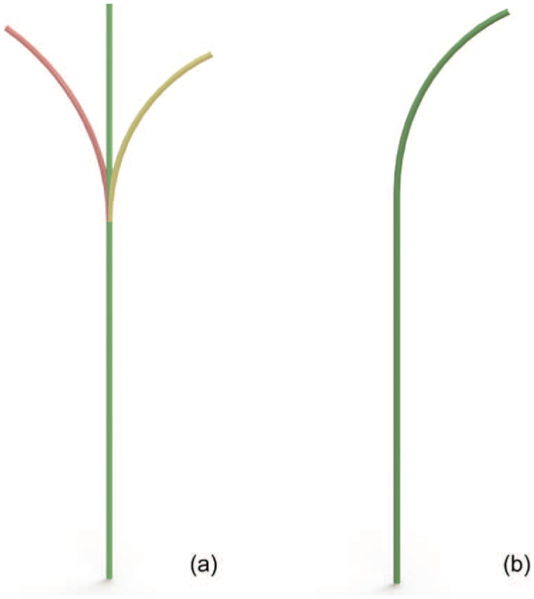
Idle tubes concept corresponding to: (a) two tubes (red and yellow) with opposite curvatures, resulting in a straight geometry (green) useful for insertion; (b) the same tubes with aligned curvatures, which corresponds to an active configuration with bending in the segment near the distal end.
Once the robot is inserted, the idle tubes can be activated by modifying their relative rotation or insertion, as shown in Figure 3(b). The active tubes only present curvature in the segment near the distal end, which is determined by their design. The result is the possibility of general motion at the robot’s distal end once inserted, while maintaining a follow-the-leader configuration throughout the rest of the robot. The general motion achievable at the distal end is determined by the geometry of the idle tubes, which is selected by design. As in the previous subsections, the idea of using idle tubes has been proposed previously in the literature. Here, the idea is generalized to the precurvatures and trajectories discovered in this paper, and the concept is extracted from the analysis in the previous sections, leading to a more complete study.
The advantage of using idle tubes relative to the maneuvers described in the previous subsection is that idle tubes do not impose any restrictions on their control, since their proximal part is straight. Conversely, idle tubes cannot contribute to the follow-the-leader kinematics, unlike the groups of tubes described in the previous subsection. In this regard, idle tubes lead to a noticeable increase in robot stiffness, requiring higher precurvatures in the robot design to follow a specified trajectory. This results in devices prone to torsional instability, which is discussed in Section 5. Thus, the practical applicability of the idle tubes concept is relatively limited.
5. Torsion
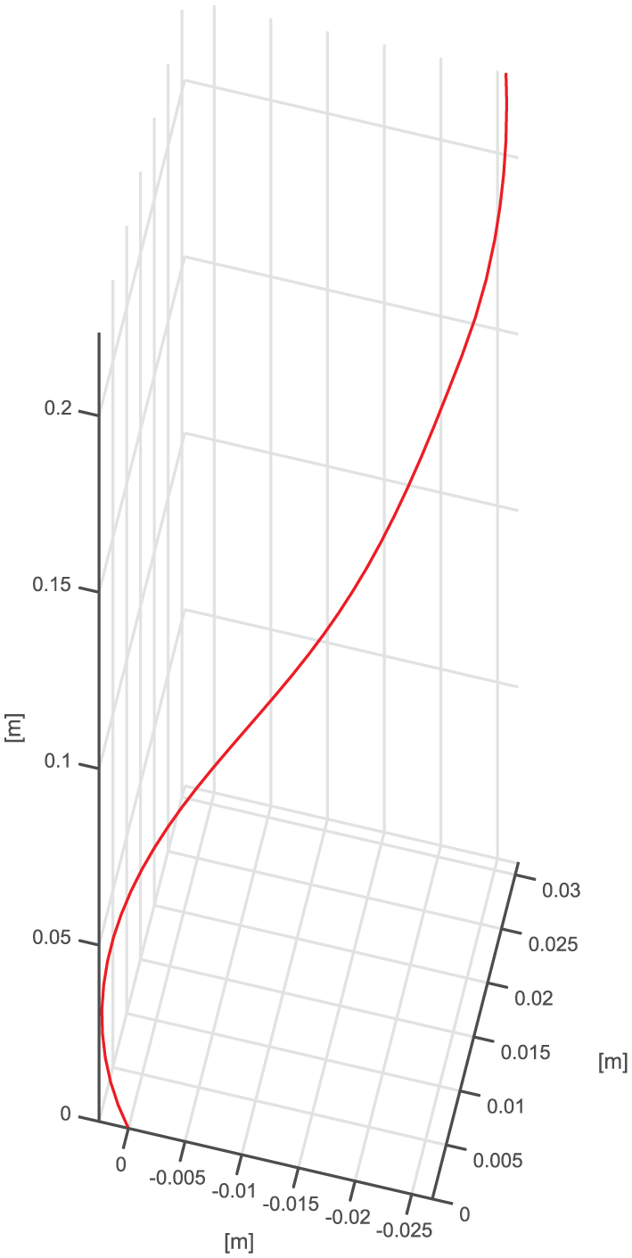
The analysis presented in the previous sections is predicated on the assumption of no axial torsion of the tubes composing the robot. Such an assumption can be used in the kinematic study of concentric tube robots, and it leads to the solutions described in previous sections. However, a certain degree of torsion is generally present in concentric tube robots, and therefore a certain deviation from follow-the-leader can occur in the trajectories previously identified. When torsion is significant, concentric tube robots can even become unstable in some of the previously identified trajectories, owing to the so-called snap-through instability described in Dupont et al. (2010b). Thus, even though some of the trajectories found under the assumption of no torsion can be tempting, as that shown in Figure 4, they may not be viable.
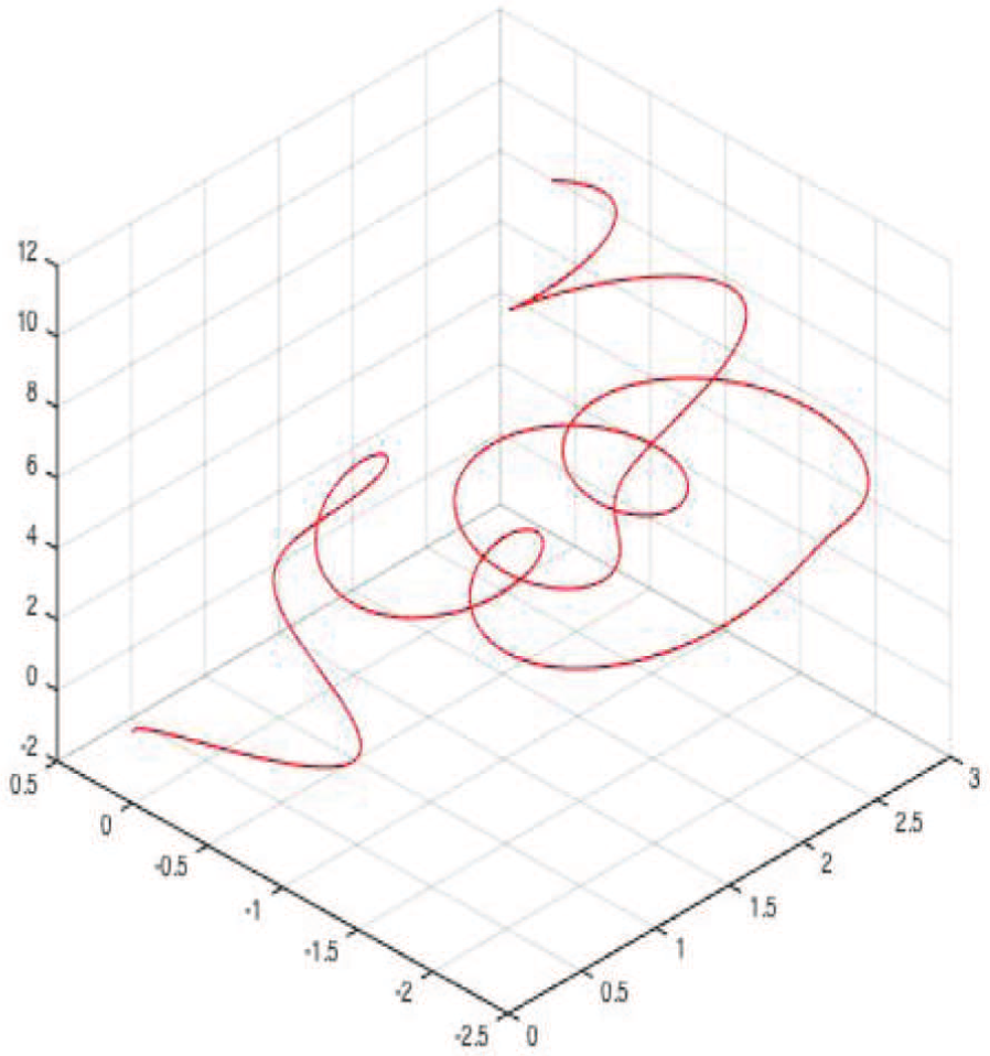
Example of trajectory from the set (equation (24)), illustrating the fact that the assumption of no axial torsion can lead to intriguing predictions, but a study of torsion is required to determine feasibility.
The torsion of concentric tube robots is studied in this section to determine the validity of the assumption of no axial torsion, and therefore allow for the selection of robot configurations where such an assumption is an acceptable approximation. The study of torsion requires a general equilibrium analysis, which is derived in this section using special Cosserat rod equilibrium theory, following the approach in Dupont et al. (2010b). The study is then made specific to trajectories of interest in Subsection 5.2, and a closed-form solution for a two-tube robot is presented. The implications of such a solution are subsequently discussed in Subsection 5.3, and criteria to ensure that the torsion of the tubes is less than a specified value are extracted. The relation between torsional deformation and deviation in task space is illustrated with some cases of interest in Subsection 5.4, serving for the selection of a robot design for the case study described in Section 6.
5.1. General formulation of torsional study
The derivation of the general differential equation governing torsion presented in this subsection is analogous to that in Dupont et al. (2010b). However, the main steps of the derivation are included for completeness, serving as a foundation for the subsequent analysis in this paper. To facilitate the integration of this work with existing literature, a new variable is defined, ζ = L – s, which corresponds to the arc length relative to the robot’s proximal end. The study of torsion in the following is derived using ζ as the independent variable.
The equilibrium of a tube i subjected to distributed external forces
where
In this work, the focus is on the robot equilibrium resulting from the interaction between tubes. Thus,

Considering the derivative of the constitutive relation (equation (1)) with respect to arc length
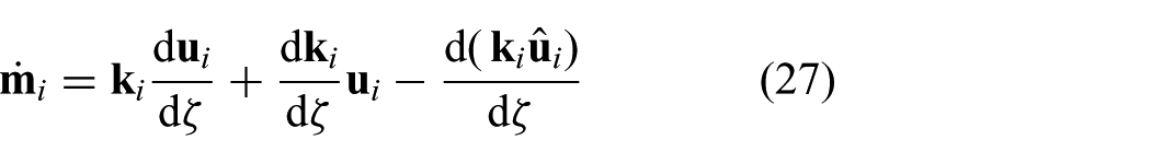
and combining equations (26) and (27) yields
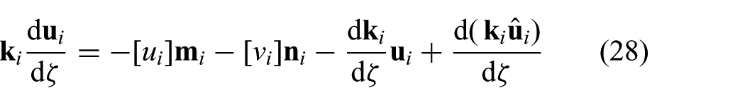
The angular strains can be assumed to be the prevailing deformation modes over linear strains, following Dupont et al. (2010b), leading to
Recalling that the initial curvature of a tube is defined in Section 2 as the curvature of the curve corresponding to its centerline, the z component of
which describes the torsional derivative of a tube with respect to ζ as a function of its initial and deformed bending curvatures. It should be noted that this expression is equivalent to that presented in Dupont et al. (2010b), as it is applicable to any concentric tube robot design under the aforementioned assumptions.
Considering a robot composed of two tubes, the relative twist angle can be defined as

where
The variables
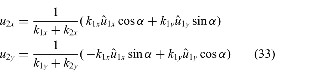
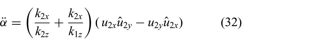
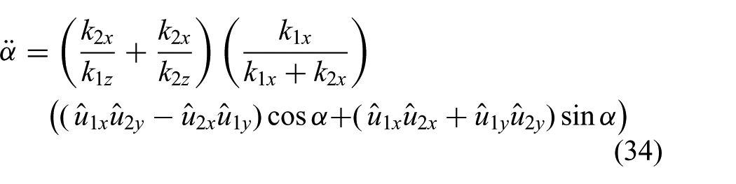
Substituting equation (33) into equation (32), and after some manipulation, including the aforementioned assumption that
A first boundary condition can correspond to the twist at the proximal end of the robot, i.e. at

The second boundary condition can be obtained by considering that the torsional moment at the distal end of each tube must be zero, which implies no torsion of the tubes at ζ = L and therefore

It should be noted that equation (34), together with the boundary conditions (equations (35) and (36)), is general, and therefore valid for any two-tube robot design satisfying the assumptions used in the derivation.
5.2. Torsion in particular configurations
Equation (34) can be made specific to trajectories in the set (equation (24)) in order to determine the validity of the assumption of no axial torsion in practice. The most relevant trajectories in practice are those corresponding to tubes compensating individually since they only require one tube per component in equation (24), which enables a wide variety of non-trivial trajectories to be followed with a small number of tubes, and they offer lengths and curvature values of typical practical interest. The following derivation is thus focused on robots composed of tubes with helical precurvatures. Substituting these helical precurvatures from equation (24) into equation (34), and after some manipulation

where
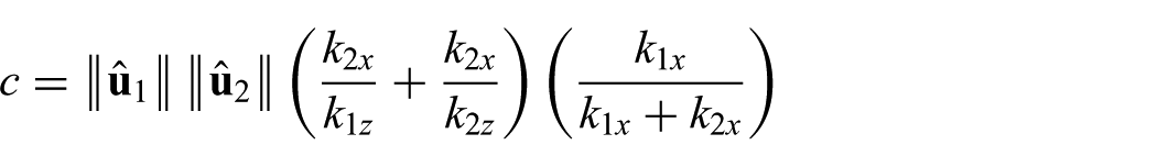
in which

equation (37) transforms into
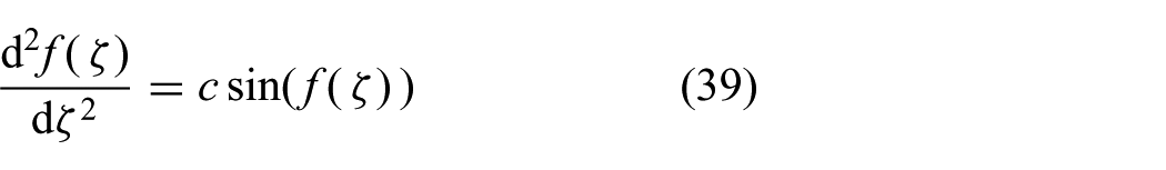
with boundary conditions
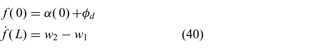
Equation (39), with boundary conditions (40), is similar to that obtained in Dupont et al. (2010b), but differs in one of the boundary conditions, requiring a different solution. The solution to equation (39), and its application to solve equation (37) by reversing the change of variable in equation (38), are derived in Appendix B.
Thus, defining
and
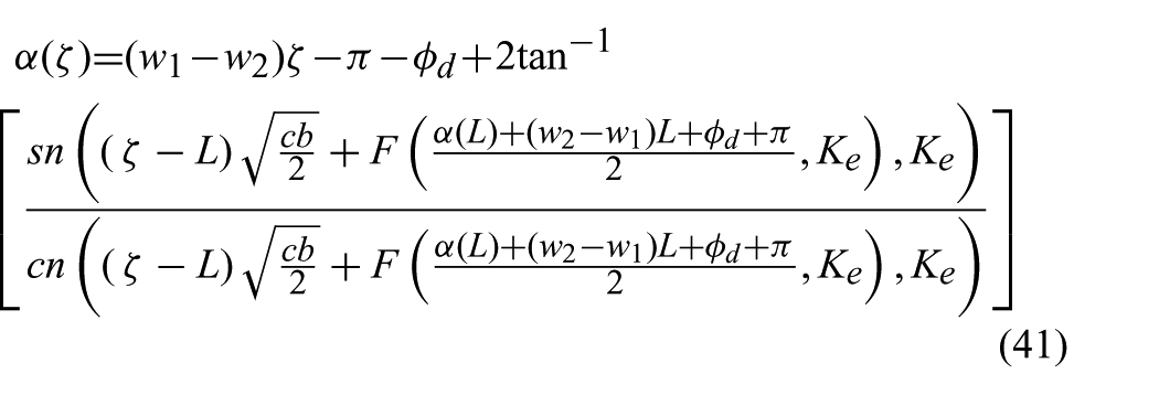
where F(x,K) denotes the incomplete elliptic integral of the first kind, and sn and cn correspond to the Jacobi elliptic functions. And for
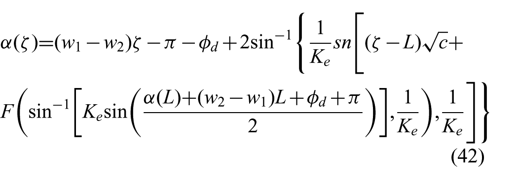
where the transition at
It should be noted that the solution is expressed as a function of the relative twist at the distal end of the robot, instead of the proximal end as in the boundary condition (equation (35)). An equivalent result can be obtained using α (0) as the independent variable instead of α (L) following an analogous derivation. However, α (L) is selected as the independent variable in this case since it facilitates the discussion on torsional stability, which is the final aim of this torsional study.
5.3. Torsion discussion
The implications of equations (41) and (42) are analyzed in this subsection. The focus is on the torsional magnitude in order to determine the validity of the assumption of no axial torsion employed in the previous sections of this paper, and thus identify stable trajectories.
Equations (41) and (42) allow the determination of the relative twist at any cross-section of a two-tube robot composed of helical tubes as a function of α (L) as well as the robot design parameters and
Three illustrative examples of different relations between α (0) and α (L) are shown in Figure 5, which correspond to three different cases in terms of values of the non-dimensional groups. Ascan be seen, for two of the cases, the evolution of α (L) as a function of α (0) is stable, whereas in the third case the robot presents a torsional instability corresponding to a snap-through instability. The two stable examples, however, present markedly different evolutions of relative twist. The relation shown in blue is strongly non-linear, which implies that the assumption of no axial torsion is not an accurate representation of the torsional behavior. Instead, the relation shown in green is closer to linear, and therefore can be approximated well by the assumption of no axial torsion of the robot.
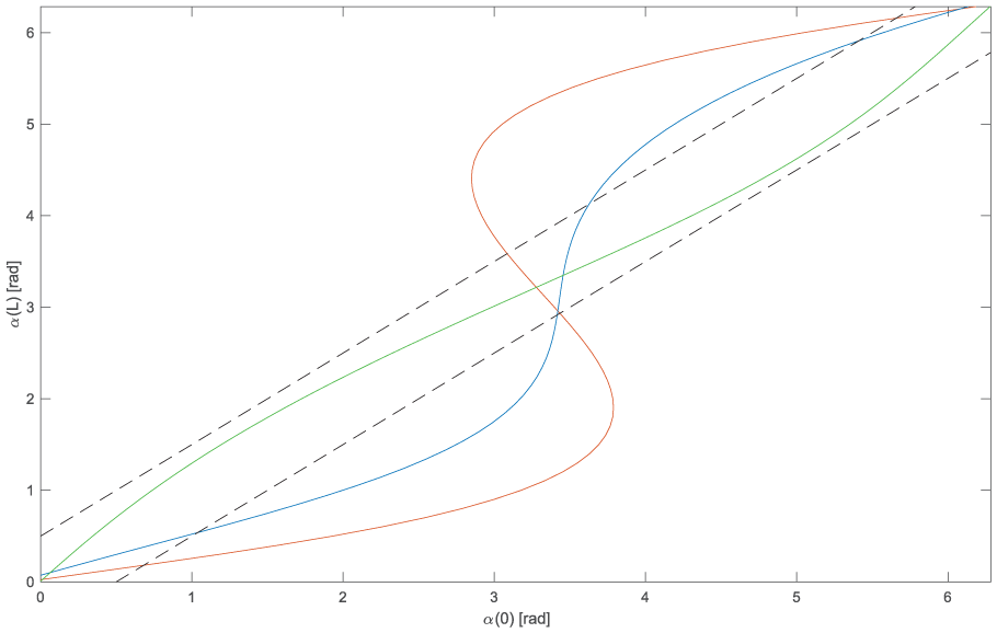
Evolution of the relative twist between the distal and proximal ends of robots composed of two tubes with three different designs, which present a stable and approximately linear relation (green), a stable but non-linear evolution (blue), and an unstable behavior in the interval α (0) ∈ [2.8, 3.8].
Studying the evolution of α (L) as a function of α (0) for a range of values of the non-dimensional groups in combination with equations (41) and (42), criteria to attain a desired torsional behavior can be extracted. The domain considered here is selected to include the configurations of practical interest, with
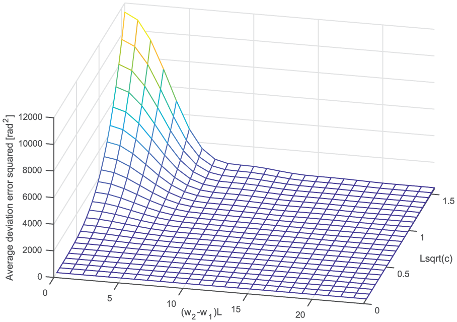
Average squared deviation from
A torsional deviation in the relation between α (0) and α (L) can therefore be selected to be less than a specified value in order to ensure that the assumption of no axial torsion is an acceptable approximation. It should be noted, however, that a boundary on torsional deformation does not directly imply a specific boundary on the deviation with respect to follow-the-leader motion in the resulting trajectory. The torsional deformation affects the local curvature values, whereas the deviation in the resulting trajectory is determined by the integration of the local curvature along the robot length. Thus, torsional deformation and resulting deviation in task space are related, but the relation depends on an integral.
Equations (49) and (50) can be substituted into the well-known robot model including torsion, e.g. that described in Dupont et al. (2010b), to determine the deviation in local curvature due to torsion in a two-tube robot. This can then be particularized to the robot designs and configurations found in this work to determine the local curvature deviation in the trajectories of interest (equation (24)). However, to determine the resulting position deviation due to torsion in task space, the local curvature needs to be integrated. A closed-form solution to such an integral is not available. Thus, the specific deviation in task space due to torsion cannot be directly determined from the current analysis. The possibility of approximating this integral or finding boundaries on the deviations in task space from boundaries on local curvature deviations will be addressed in future work.
Nonetheless, in some practical cases, the typical deviation in task space due to torsional deformation can be considered to follow certain trends that can be approximated for a specific family of designs based on experience. In such cases, boundaries on torsional deformation can be used to identify the trajectories where follow-the-leader is possible within an admissible deviation. To exploit any trajectories of interest, however, these must be subsequently verified to ensure that the deviation in task space is within the expected values. In more general cases, a hypothesis on the admissible torsional deformation in the specific scenario of interest can be formulated by exploring the effect of torsion on the resulting trajectory in some relevant configurations. The corresponding trajectories where approximate follow-the-leader is possible can then be identified, and trajectories of interest can be selected. However, any selected trajectory must be subsequently verified. This procedure can, therefore, require some iteration. In all cases, it should be noted that boundaries on torsional deformation typically involve using tubes with lower curvatures. In particular, in designs composed of tubes with planar precurvatures, this always applies, as torsionaldeformation is determined by a single parameter,
5.4. Illustration of torsion effects
A set of examples of torsional deformation and the corresponding deviations in task space are presented in this subsection. These are aimed at illustrating the relation between torsion and the resulting deviation for some designs of interest.
Three simulated insertions are first used to show the behavior of three exemplary robot designs corresponding to the torsional relations shown in Figure 5, and then to quantify the follow-the-leader deviation in task space due to torsion. The simulations are implemented using the robot quasistatic model considering torsion (equation (4)) together with the solutions of torsion along the arc length (equations (41) and (42)). The robot configuration is evaluated at 10 regular intervals during an insertion. The three designs are all composed of two helical tubes with equal stiffness, a length of 20 cm, and
The resulting simulated insertions are shown in Figure 7. As can be seen, follow-the-leader is maintained in some parts of the trajectories, but significant deviations are present in both the first and second designs. In this work, the deviation, defined ϵ, is quantified as the maximum of the minimum distances between any point on the robot centerline at any of the configurations during an insertion and the centerline at any other configuration. The maximum deviations for the insertions shown in Figure 7 are then
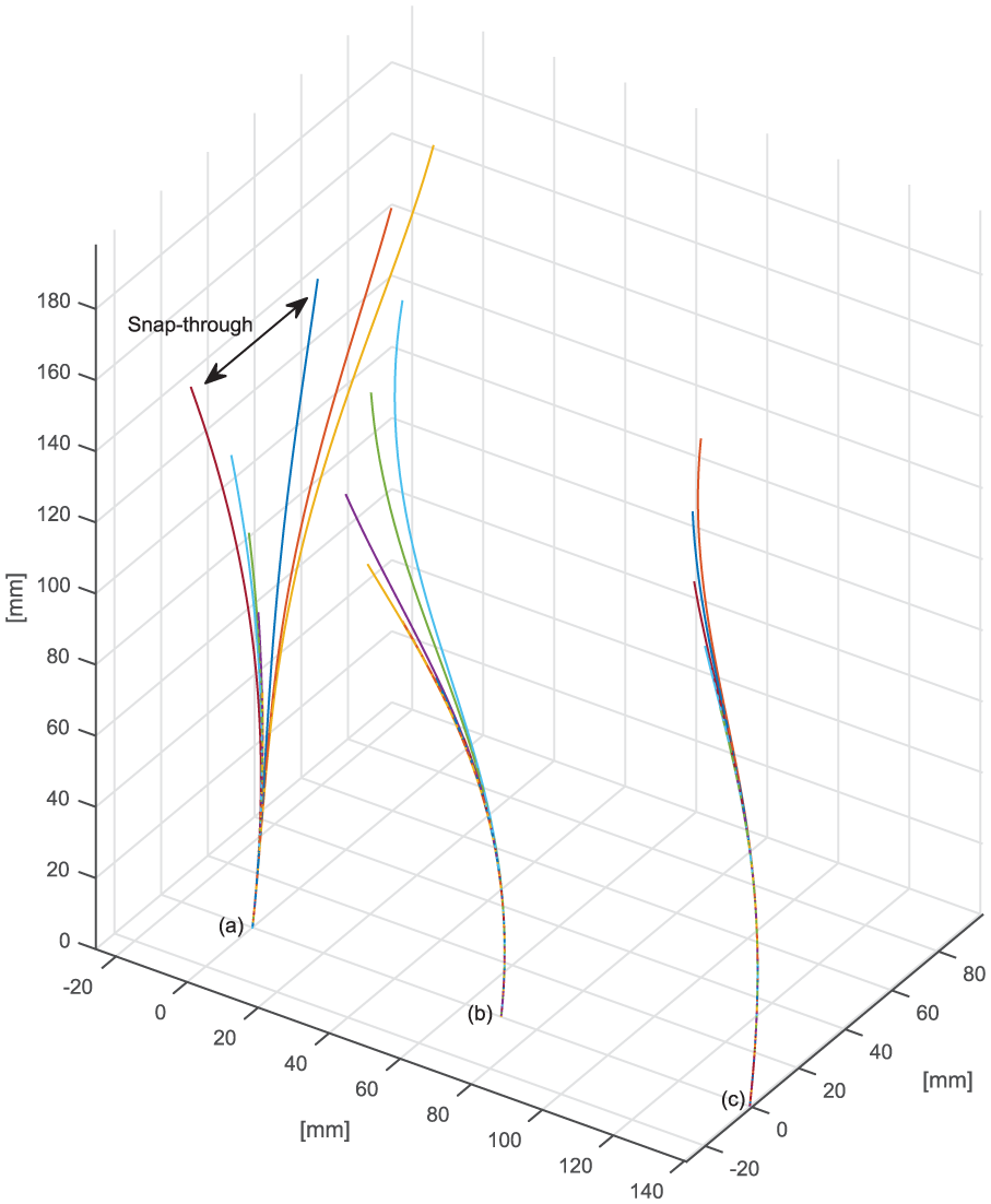
Simulated insertions corresponding to three different designs: (a) significant deviation from follow-the-leader, including a snap-through instability; (b) noticeable deviation due to torsional deformation of the tubes; (c) low deviation.
Equivalent simulations can be conducted to explore the relation between torsion boundaries and deviation in task space in any set of designs. This is presented here for a relevant subset of designs corresponding to two-tube robots with helical tubes of equal stiffness, a length of 20 cm, curvatures of each tube varied within
The maximum deviation in task space is plotted in Figure 8 as a function of the maximum torsional deviation, defined as
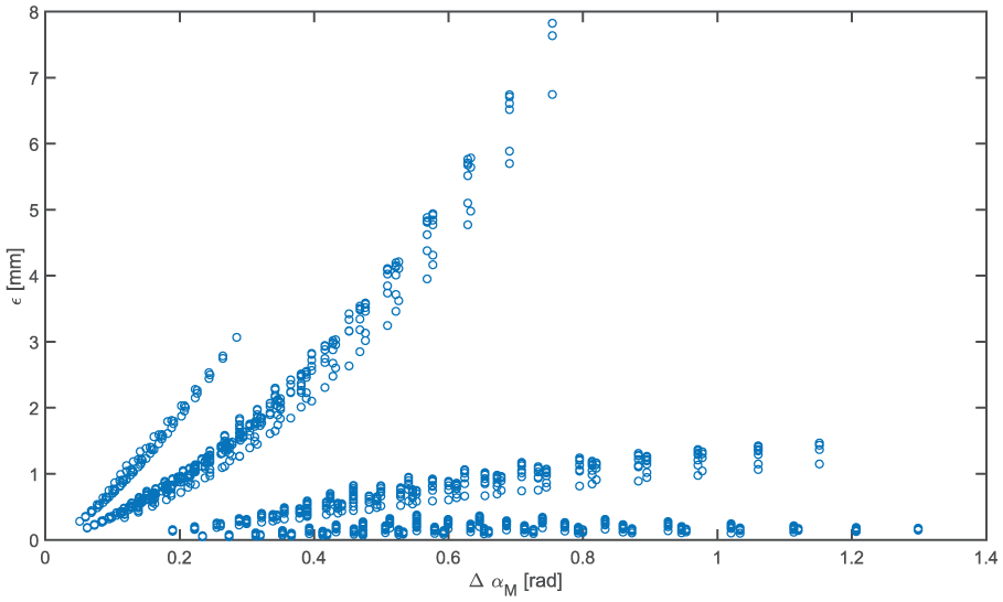
Maximum deviation from follow-the-leader in task space as a function of maximum torsional deviation for a wide variety of designs.
Torsion boundaries can then be defined in the subset of designs explored so that the assumption of no torsion is an admissible approximation, and thus the corresponding follow-the-leader trajectories can be followed within an acceptable deviation. This can be exemplified by considering admissible the relations between α (0) and α (L) that lie within two boundaries depicted as dashed lines in Figure 5, and without snap-through. These boundaries are arbitrarily set to be parallel to α (0) = α (L) with an offset of ± 1∕2 m−1, and correspond to maximum deviations in the task space of close to 4 mm. It should be noted, however, that these bounded deviations are only guaranteed in the specific configurations explored. Deviations on any other configuration, even if similar, must be verified.
The trajectories corresponding to the configurations explored within these bounds are plotted in Figure 9 for a common initial pose at the base. It should be noted that the trajectories shown in Figure 9 can also be rotated around the base z axis while maintaining the base pose, increasing the follow-the-leader possibilities for that pose, although they are not plotted, for clarity of illustration. It should also be noted that equations (41) and (42) do not depend on the length units in the robot design variables; therefore, any isotropic scaling of the trajectories shown in Figure 9 results in a trajectory that can also be traced in an approximate follow-the-leader manner with a deviation that scales with L. Figure 9 illustrates the potential of the trajectories discovered in this work for surgical applications, showcasing the capability of following trajectories with a continuous variation of curvature, in both magnitude and direction, in an approximate follow-the-leader configuration to reach targets in different locations from a specified initial pose.
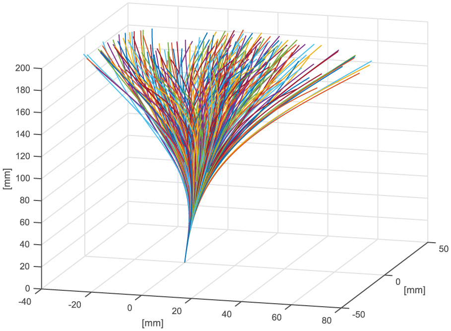
Set of stable trajectories where follow-the-leader is possible using a robot composed of two tubes, with a common base pose.
6. Case study: simulation and experiment
The results on torsional stability presented in the previous section allow for the selection of a robot design together with a trajectory to showcase the research reported in this paper. The performance of the selected robot is presented in this section in the form of a case study involving simulation and experiment. This serves to illustrate both the capability of follow-the-leader motion in a trajectory that is unique and representative of the research on follow-the-leader control, as well as the validity of the assumption of no axial torsion in such a trajectory.
6.1. Robot design and trajectory
The case study involves a two-tube robot advancing in follow-the-leader motion along a trajectory with continuous variation of curvature, in both direction and magnitude, in the proximal part of the trajectory, and a helical geometry in the distal part. The trajectory selected is a combination of two trajectories in the set (equation (24)) linked as described in Subsection 4.1, whereby one of the tubes remains static at the linkage between trajectories while the other proceeds forward. The case study therefore serves to demonstrate the research reported in Section 3, as well as some of the work on additional exploitable kinematics described in Section 4. The behavior of the robot in the first, proximal, part of the trajectory is studied with simulations, whereas that in the second, distal, part of the trajectory is shown with an experiment.
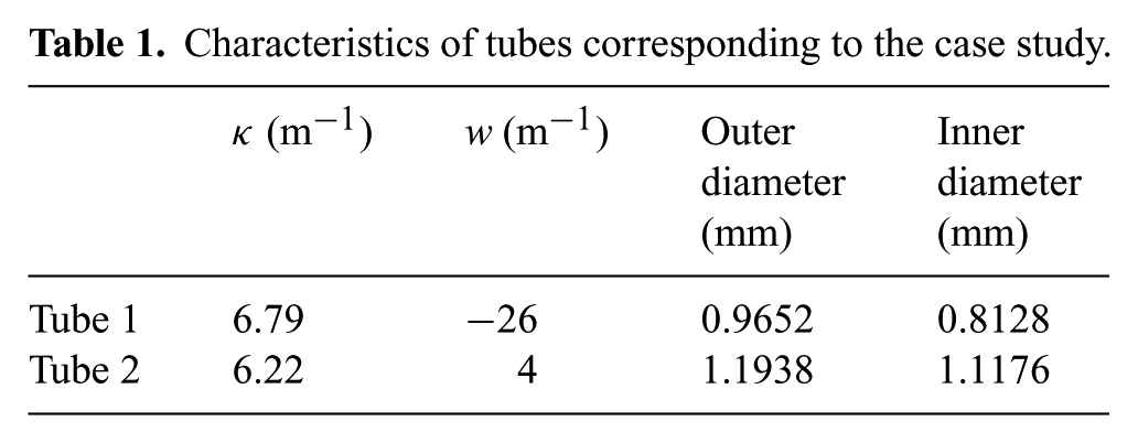
The geometry of the complete selected trajectory can be described by the curvature
Characteristics of tubes corresponding to the case study.
Complete trajectory selected for the case study. The first, proximal, part of the trajectory presents continuous variation of curvature in both direction and magnitude; the second, distal, part of the trajectory presents a helical geometry.
The tube’s characteristics are selected to minimize torsion. The evolution of α (L) as a function of α (0) can be predicted using equations (41) and (42), as shown in Figure 11. In this case, the design parameters summarized in Table 1 result in the approximately linear relation between α (L) and α (0) shown in Figure 11. Thus, torsion is expected to be low in the entire trajectory.
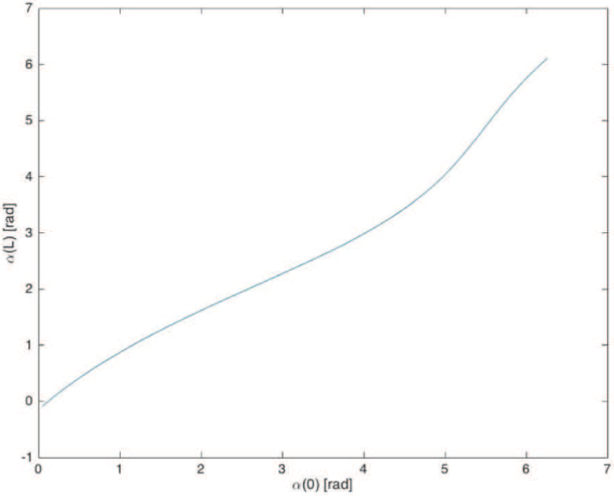
Predicted evolution of the relative twist at the distal end as a function of the proximal end of the robot design selected for the experiment.
6.2. Simulation
The first part of the trajectory corresponds to both tubes advancing with
The geometry of the robot in each of these 20 configurations is simulated as in Subsection 5.4, by combining equations (4), (41), and (42). The effects of friction between tubes and gravity are neglected, and the tubes are assumed to be made of nitinol with a Poisson ratio of ν = 0.33.
The desired control inputs at the insertion point for this part of the trajectory are determined from equation (20) with
The resulting simulated robot configurations are shown in Figure 12. As can be seen, an approximate follow-the-leader motion is maintained over this entire firstpart of the trajectory, although a certain degree of deviation is present. The deviation from follow-the-leader is relatively low near the insertion point and increases toward the distal parts of the trajectory. The maximum deviation in task space, quantified as in the previous section, is 3.5 mm, and occurs between the configurations at 85% and 100% of the insertion, at an arc length of 163.9 mm of the final configuration.
Simulated insertion of robot in the first part of the trajectory.
The deviations shown in Figure 12 are due to torsion. The simulated torsional deviation along the arc length Δα(ζ) = α(ζ) − α(0) is shown in Figure 13 for the robot configurations corresponding to the 20 insertion lengths. As can be seen, the torsional behavior varies as the insertion of the robot increases, which results in changes in the local curvature along the arc length, and ultimately leads to deviations from follow-the-leader in task space. The relation between deviations in local curvature and follow-the-leader error in task space is determined by the integration of curvature along the arc length, and therefore the effect of local curvature deviations is amplified with the arc length, which results in the larger errors in the distal parts of the trajectory shown in Figure 12.
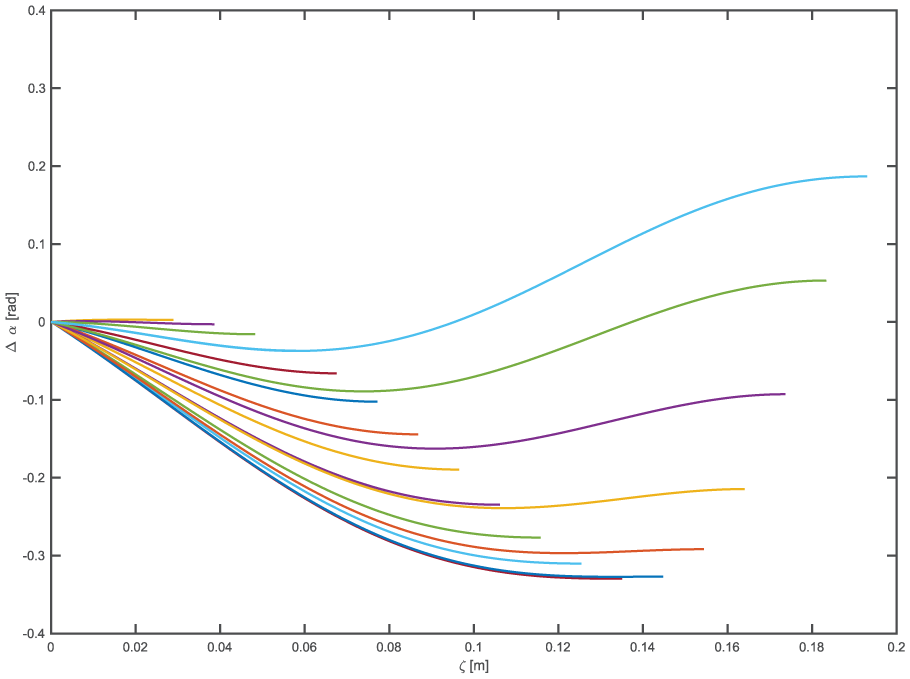
Simulated torsional deviation as a function of arc length for 20 robot configurations during an insertion.
6.3. Experiment
The second part of the trajectory is a continuation of the first one. It begins with both tubes inserted as described in the previous subsection. One of the tubes is then advanced to trace this second part of the trajectory while the other tube remains stationary relative to the task space. The robot behavior in this second part of the trajectory is demonstrated experimentally to illustrate follow-the-leader motion in practice.
The experiment starts with the distal end of both tubes coinciding, which corresponds to the end of the first part of the trajectory. Tube 1 is subsequently advanced, which involves a combination of insertion and rotation of the tube at a rate of w1 m−1, while tube 2 remains stationary. The geometry of the complete device is measured as tube 1 advances in order to evaluate the satisfaction of follow-the-leader motion over the entire device. The experiment proceeds until full insertion of tube 1, which corresponds to the end of the complete trajectory shown in Figure 10.
The design of the tubes used in the experiment matches the description in Subsection 6.1, summarized in Table 1. Both tubes are made of nitinol, supplied by Nitinol Devices and Components Inc., with part numbers TSE0380X0320GS and TSE0470X0440GS, respectively. It should be noted that the stiffness of both tubes is practically equal, which requires the result in equation (24) to be correct for follow-the-leader motion to occur throughout the entire robot.
Starting the experiment from the point of linkage between the two parts of the complete trajectory enables follow-the-leader motion to be achieved without the need for an actuation system. Tube 1 can be simply advanced with free rotation, relying on the elastic equilibrium of the system to rotate it naturally at the required rate w1.
This rotational behavior is necessary in this configuration, corresponding to follow-the-leader, where the curvature at each point in the workspace must be constant. For tubes with constant stiffness, as in this experiment, follow-the-leader requires the curvature vector of each tube to remain constant at each point in the workspace. Since the tubes are in a minimum energy equilibrium at the beginning of the experiment, tube 1 is expected to rotate to remain in the minimum energy equilibrium as it is being inserted. Considering that the tubes have a helical geometry, remaining at a minimum energy configuration implies maintaining a constant-curvature vector at each point in the workspace, and therefore rotating at the follow-the-leader rate w1. This structural behavior can therefore be exploited to design a simpler experiment that suffices to illustrate the research on follow-the-leader, which is the strategy adopted in this work for the implementation.
The experimental set-up used in the implementation is shown in Figure 14. The shape of the device is measured at regular intervals during advancement using a 3D laser scanner (PICZA LPX-250, manufactured by Roland). The desired initial geometry of the tubes was achieved by means of a shape-setting process. Since the tubes’ stiffness is constant, their precurvatures are helical, and the shape-setting process simply involved constraining each tube to a cylindrical fixture of the specified diameter, heating the assembly in air to
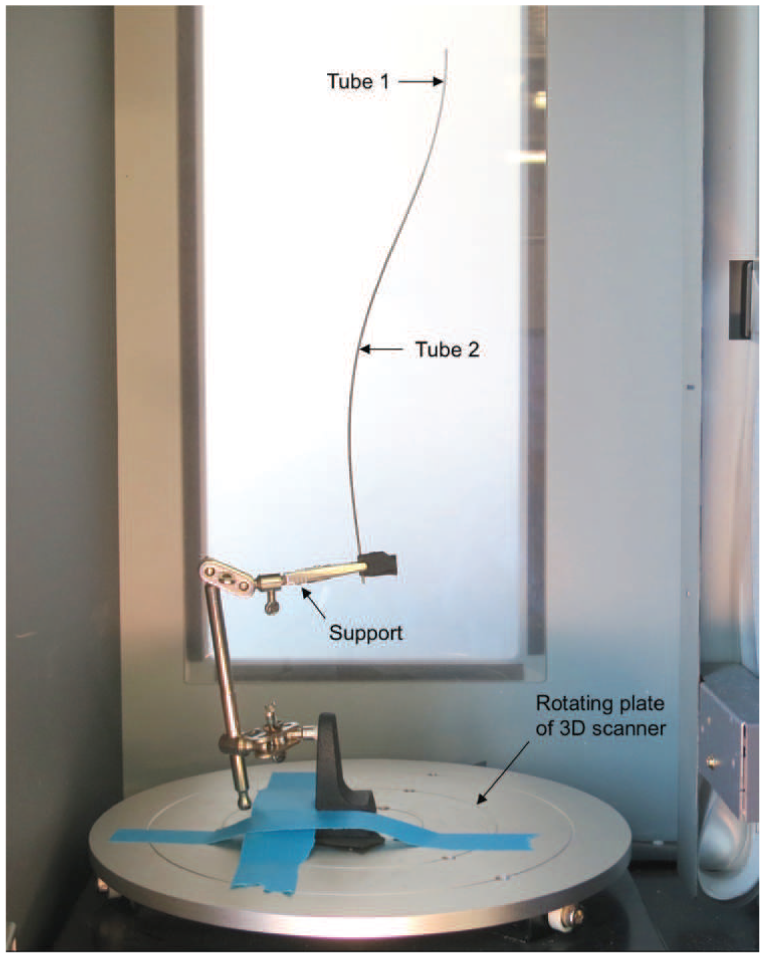
Experimental set-up with device held vertically inside 3D laser scanner.
Six robot shape measurements were recorded using the 3D laser scanner as tube 1 was advanced. Each measurement consists of a set of points describing the device shape, as shown in Figure 15 for the third measurement, with the corresponding projections on the XZ and YZ planes, shown in Figures 16 and 17, respectively. A curve is fitted to determine the geometry of the curve corresponding to the device centerline, which is also shown in Figures 15 to 17, for the same measurement. As can be seen, the measurement presents a certain degree of noise, which is mainly caused by the vibrations induced in the device by the rotation of the 3D scanner. The noise is zero mean, and the fitted curve allows for reliable extraction of the geometry of the device. The fitted curves of the different measurements are subsequently used to assess the follow-the-leader motion.
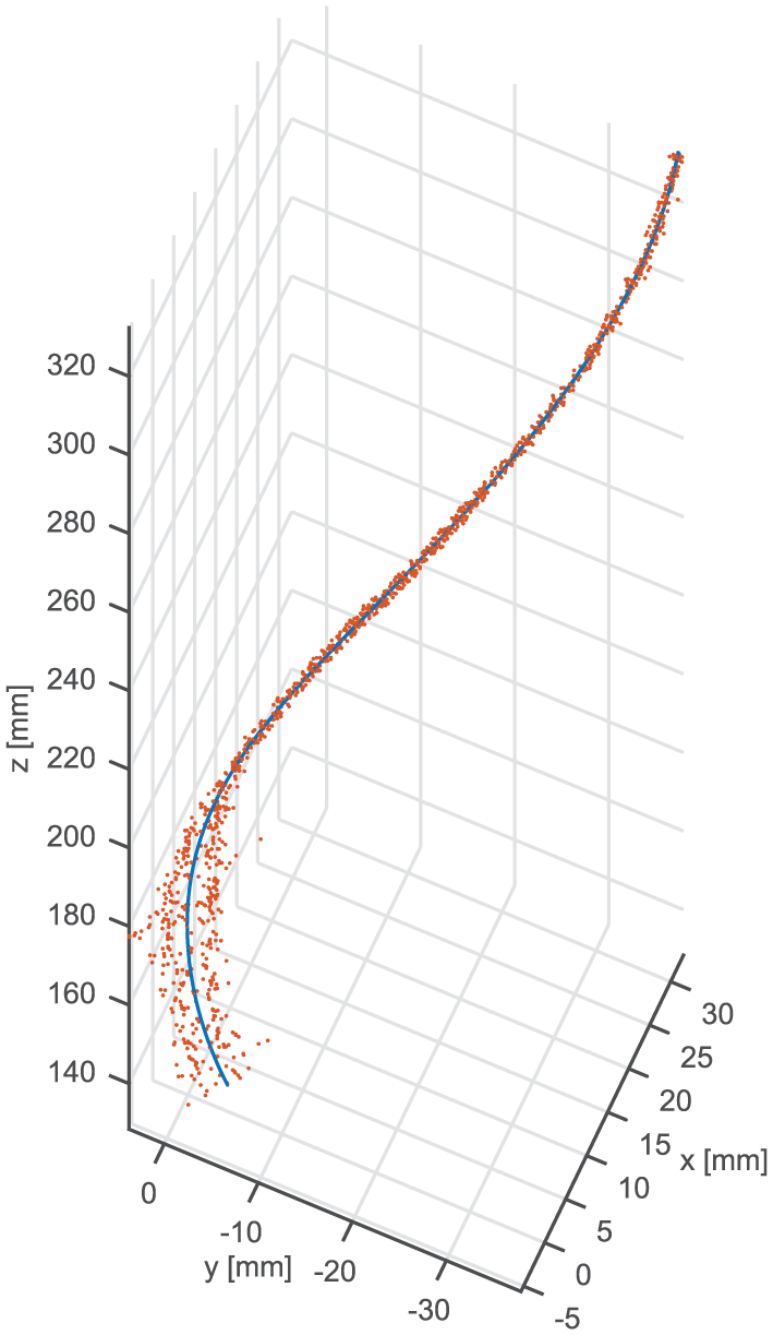
Exemplary measurement of the 3D device geometry as a cloud of orange points, with a fitted 3D curve in blue.
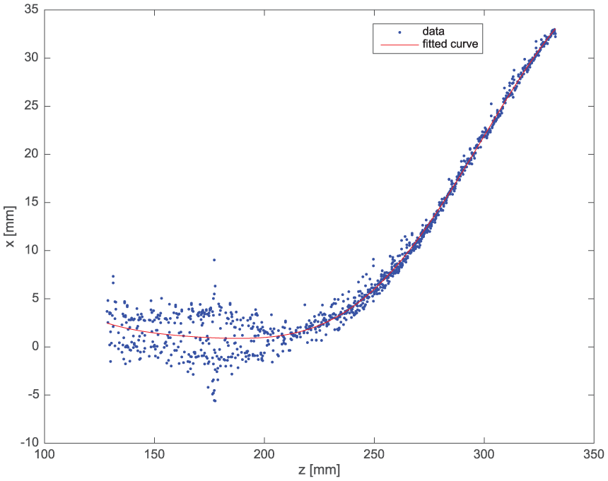
Projection on the XZ plane of the recorded points describing the geometry of the device in one exemplary measurement, with the corresponding fitted curve.
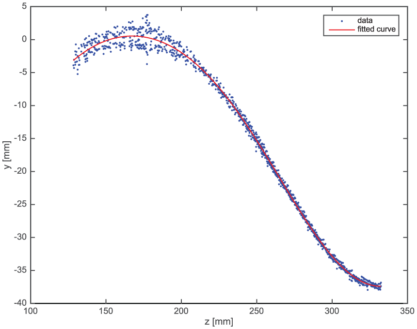
Projection on the YZ plane of the measured points corresponding to the device shape in a specific configuration during the experiment, and fitted curve.
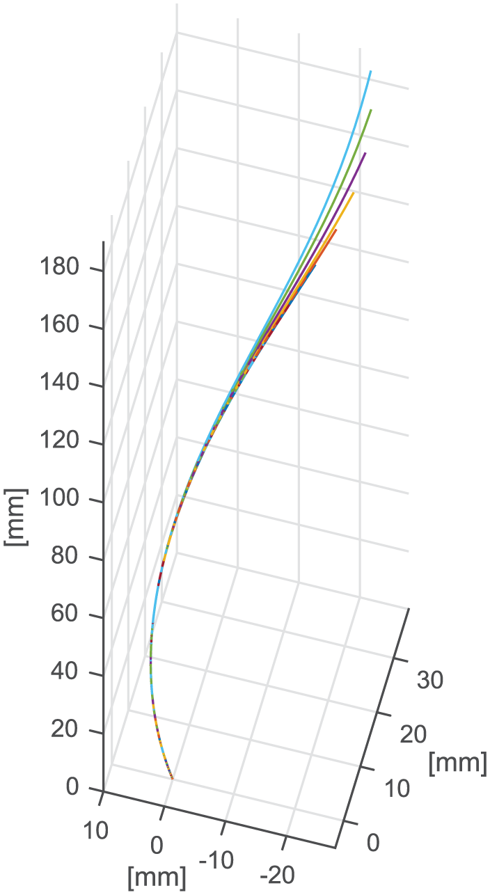
The result of the experiment is an accurate follow-the-leader configuration throughout the entire device. The 3D points from the different measurements recorded during device advancement, together with their corresponding fitted curves, are shown in Figure 18, using specific colors for each measurement. The projections of the fitted curves on the XZ and YZ planes are shown in Figures 19 and 20, respectively. As can be seen, the motion in both parts of the trajectory, corresponding to two tubes and one tube, remains within a follow-the-leader configuration. The maximum deviation estimated from the fitted curves in each measurement is 4 mm. This can be partially attributed to the limited accuracy of the experimental set-up, 3D scanner, and shape-setting process, as well as small discrepancies between the idealized robot behavior and the practical implementation, mainly in terms of external forces or friction between the tubes.
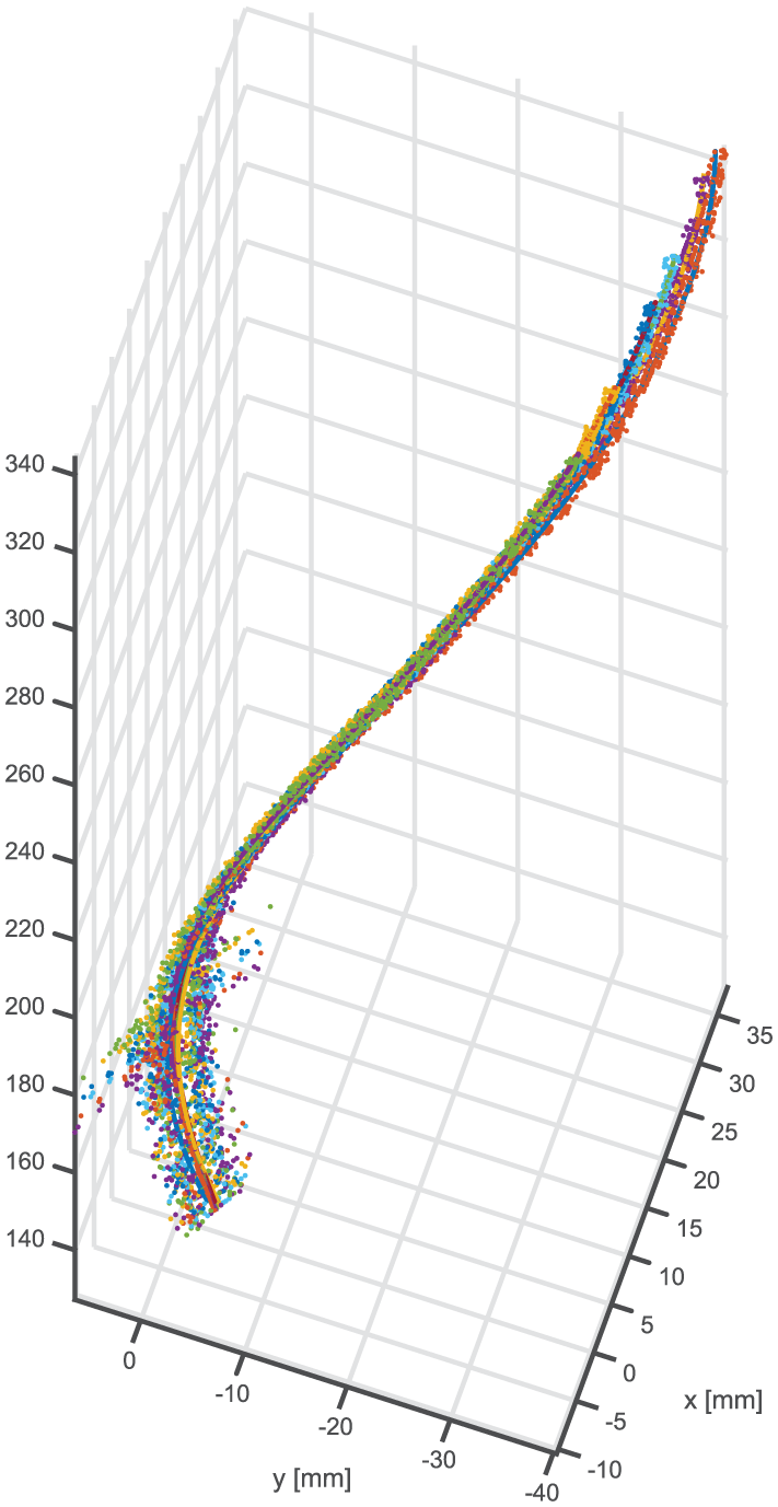
Experimental measurements of the device geometry during the advancement of one of the tubes, plotted as a point cloud with a different color for each recorded configuration. The different measurements overlap, confirming follow-the-leader motion throughout the entire device. The curves fitted to each measurement are also displayed.
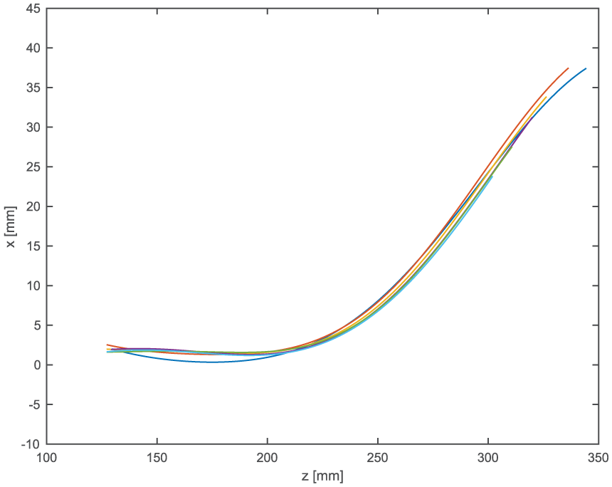
Projection on the XZ plane of the curves fitted to the experimental measurements during advancement of one of the tubes.
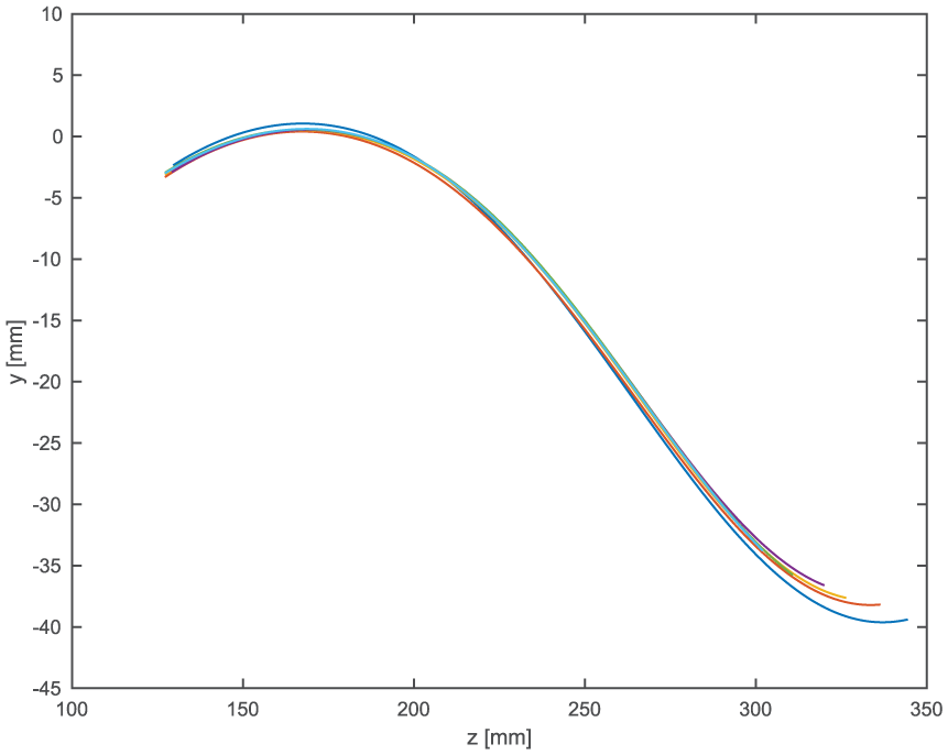
Projection on the YZ plane of the curves fitted to the experimental measurements during advancement of one of the tubes.
The trajectory displayed by the device in the experiment presents the same approximate characteristics as the planned trajectory, as shown in Figure 21, although there are some discrepancies. The discrepancies are considered to be related to imperfections in the experimental implementation, as well as small inaccuracies in the assumptions used in the derivation. Interestingly, in the experimental implementation, tube 1 presented an estimated rotation at the expected rate as it was being inserted, according to visual observation of the rotation at the base of the tube aided by markers. The apparent torsion of the tubes, also estimated from visual observations at α(0) and
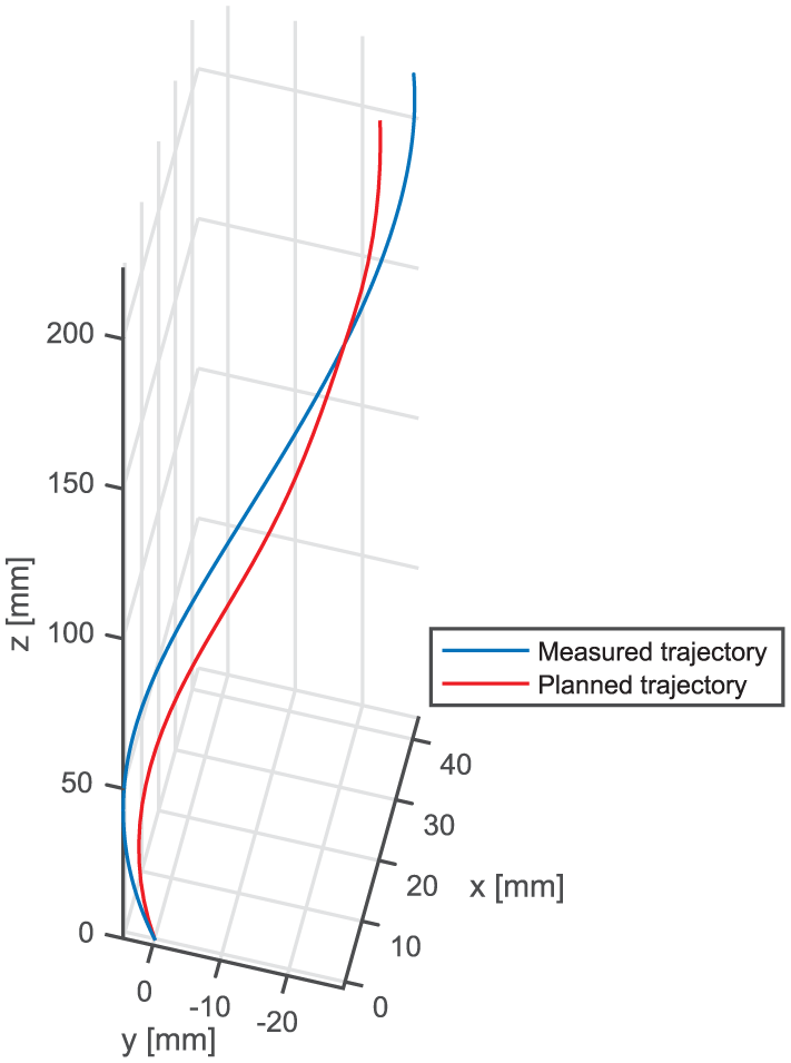
Planned and measured trajectories.
7. Conclusions
Follow-the-leader motion using concentric tube robots is possible in a broader set of trajectories than those currently being exploited. The complete set of trajectories where follow-the-leader motion is possible under the assumption of no axial torsion within the robot was derived in this work, yielding a closed-form solution. The solution obtained showed that the majority of trajectories in the set present a continuous variation of curvature along the arc length, in both direction and magnitude; still, the solution includes all currently known piecewise constant-curvature trajectories as a particular case. The analysis presented in this paper also elucidated the control required for a robot to advance in a follow-the-leader configuration, where the individual tubes must either be static or advancing as part of the robot’s distal end. Furthermore, additional maneuvers of interest were extracted from the study of follow-the-leader kinematics. These include the possibility of combining follow-the-leader motion in the proximal part of the robot with general motion at the distal end, or the linkage of trajectories that can be traced in follow-the-leader configuration. The general analysis of follow-the-leader motion was developed under the assumption of no axial torsion of the tubes. To determine the validity of such an assumption, and then select a stable robot configuration to showcase follow-the-leader motion in practice, the torsion of the tubes was considered in the trajectories of interest. A closed-form solution describing the torsion of the tubes in the most relevant trajectories where follow-the-leader is possible using two-tube robots was derived. Criteria for the structural stability of the robot were then extracted from such a solution, and a relevant subset of designs was explored. This allowed for the identification of stable trajectories that can be traced in follow-the-leader motion within an admissible deviation value, which can be specified as desired. A suitable stable trajectory was selected as a case study of a prototypical, two-tube concentric tube robot. The case study was developed with simulations and an experiment, showcasing the capability of follow-the-leader motion in a trajectory with continuous curvature variation, in both direction and magnitude. This capability in the wider set of trajectories found in this work expands the potential of concentric tube robots in minimally invasive surgery, offering the possibility for new or improved procedures.
Footnotes
Appendix A
The derivation of equation (32) is described here. Recalling the definition of
Combining the equilibrium of moments (equation (2)) in the z direction and the constitutive law (equation (1)), the following relation in the z direction can be obtained
Substituting equation (44) into equation (43), the twist rate between both tubes can be related to the torsion of one of the tubes
It should be noted that the twist rate can also be directly related to the torsion of the other tube using equation (44).
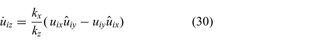
Finally, the derivative of equation (45) can be combined with equation (30), yielding
Appendix B
The derivation of the solution to equation (39) with boundary conditions (equation (40)), and its application to solve equation (37), are described in the following.
The approach adopted in this work relies on the fact that equation (39) is analogous to the equation of a non-linear pendulum. Thus, the solution to a non-linear pendulum is adapted here for the specific boundary conditions (equation (40)). Considering that
equation (39) can be integrated
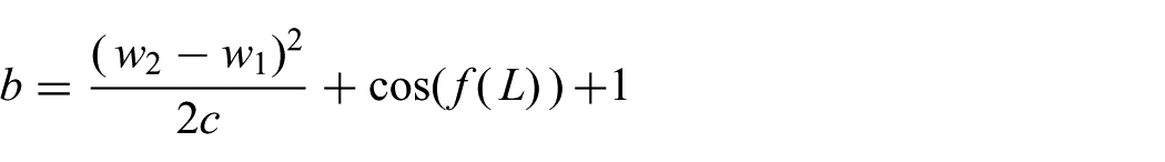
and evaluated as
This expression can be evaluated at ζ = L, considering the boundary conditions (equation (40)), and substituted in equation (48), resulting in
Using separation of variables, the integral of equation (49) can be considered in the following interval
Considering the variable definitions
This integral corresponds to the incomplete elliptic integral of the first kind F(x,K), which is defined for 0 ≤ K ≤ 1. The closed-form solution to equation (51) can be obtained in two intervals of
If
Using the Jacobi elliptic functions sn and cn, the incomplete elliptic integral of the first kind
can be inverted, which allows one to solve for h(ζ) as
If
which can be differentiated as
and guarantees that the incomplete elliptic integral is well defined. Applying such a change of variable to equation (51) yields
which can be integrated using the definition of the incomplete integral of the first kind, resulting in
Using Jacobi elliptic functions, and reversing the change of variables, equation (57) can be solved for h(ζ) as
The change of variable h(ζ) = f(ζ) + π can be reversed to obtain the solution to equation (39) from equations (53) and (58), which is immediate. Finally, reversing the change of variable (equation (38)), the solution to equation (37) can be obtained for
and for
Funding
The author(s) disclosed receipt of the following financial support for the research, authorship, and/or publication of this article: This work was supported by the Engineering and Physical Sciences Research Council [grant number EP/L015587/1], and Rolls-Royce plc.