
Abstract
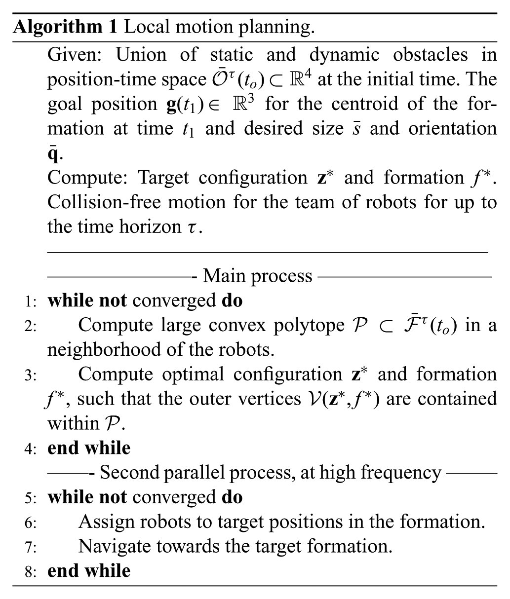
We present a constrained optimization method for multi-robot formation control in dynamic environments, where the robots adjust the parameters of the formation, such as size and three-dimensional orientation, to avoid collisions with static and moving obstacles, and to make progress towards their goal. We describe two variants of the algorithm, one for local motion planning and one for global path planning. The local planner first computes a large obstacle-free convex region in a neighborhood of the robots, embedded in position-time space. Then, the parameters of the formation are optimized therein by solving a constrained optimization, via sequential convex programming. The robots navigate towards the optimized formation with individual controllers that account for their dynamics. The idea is extended to global path planning by sampling convex regions in free position space and connecting them if a transition in formation is possible - computed via the constrained optimization. The path of lowest cost to the goal is then found via graph search. The method applies to ground and aerial vehicles navigating in two- and three-dimensional environments among static and dynamic obstacles, allows for reconfiguration, and is efficient and scalable with the number of robots. In particular, we consider two applications, a team of aerial vehicles navigating in formation, and a small team of mobile manipulators that collaboratively carry an object. The approach is verified in experiments with a team of three mobile manipulators and in simulations with a team of up to sixteen Micro Air Vehicles (quadrotors).
Keywords
1. Introduction
Multi-robot teams can be employed for various tasks, such as surveillance, inspection, and automated factories. In these scenarios, robots may be required to navigate in formation, for example, to maintain a communication network, to collaboratively manipulate an object, or to survey an area. In this work we consider two motivating applications: formation flight for teams of unmanned aerial vehicles (UAVs) in tight spaces with static and moving obstacles, and collaborative transport of large objects by multiple mobile manipulators in automated factories and working side by side with humans and other robots.
Within the field of multi-robot navigation, formation control and reconfiguration in three-dimensional dynamic environments with moving obstacles remains challenging. In this work, we leverage efficient optimization techniques, namely quadratic programming, semi-definite programming, and (nonlinear) sequential quadratic programming to address this issue. Each one is employed at different stages of the proposed method for formation control among static and dynamic obstacles. These techniques provide good computational efficiency, local guarantees, and generality. Leveraging these tools, we introduce two centralized algorithms - a local motion planner and a global path planner - that enable a team of robots to navigate in formation in two-dimensional and three-dimensional environments with static and dynamic obstacles.
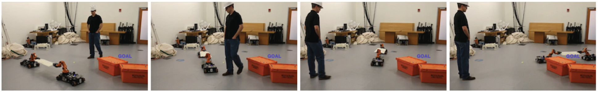
Given a set of target formation shapes, which serve as abstractions, our method optimizes the parameters (such as position, orientation, and size) of the multi-robot formation to avoid moving obstacles and make progress towards the goal. For local motion planning, an obstacle-free region, embedded in position-time space, is first grown in a neighborhood of the robots, and then the parameters of the formation are optimized, via a constrained optimization, to remain within this region. The formation optimization method guarantees that the team of robots remains collision-free and makes progress towards the goal. To make global progress towards a goal configuration, we also present a global path planner which builds a graph of feasible formations in the environment. The graph is created by a random sampling of convex regions in free space, which are kept if a valid formation exists within. A human may also provide the global path for the robots, or a desired velocity for the formation, and the robots will adapt their configuration automatically. An example of the method for mobile manipulators is shown in Figure 1. A video illustrating the results of this paper is available at https://youtu.be/sDNqdEPA7pE.
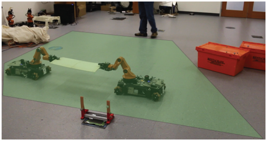
Two mobile manipulators collaboratively carry a rigid object. A projection of the obstacle-free convex region is superimposed in green.
1.1. Contribution
The main contribution of this paper is a scalable and efficient method for navigation of a team of robots while reconfiguring their formation to avoid collisions with static and dynamic obstacles. The method applies to robots navigating in 2D and 3D workspaces and contributes the following.
Locally optimal formation control. The parameters of the group formation are optimized online within the neighborhood of the robots via a centralized sequential convex optimization with avoidance constraints in dynamic environments.
A global path planner for navigating in formation. A sampling based graph-search algorithm where convex regions in free space are sampled and connected if the intersections are traversable in formation. Sampling and nonlinear optimization are combined to find a safe global path.
This work provides a working solution to a difficult problem that has not been treated at this scale before. The main strength is its ability to handle dynamic obstacles in three-dimensional environments via constrained optimization, which automatically computes the parameters of the formation to avoid collisions. Furthermore, the formation control method scales well with the number of robots, since its complexity is independent from the number of robots in the team (see Figure 2 for an example of the abstraction of the formation by its outer vertices). Finally, we validate the approach in simulations with teams of aerial vehicles and in extensive experimental demonstrations with three mobile manipulators carrying a rigid object.
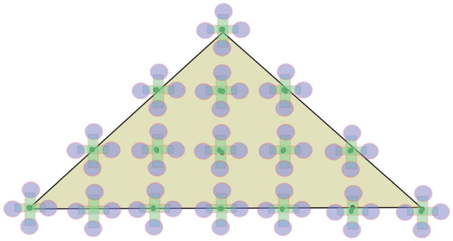
A triangular formation with sixteen aerial robots can be abstracted by a triangle defined by three vertices. The formation can also be defined in three-dimensional space.
In an earlier conference version of this work (Alonso–Mora et al., 2015a), the local motion planner was introduced. In this paper, we describe the approach in detail, we extend it for global path planning, and we present additional experiments with a team of three mobile manipulators collaboratively carrying an object.
The geometrical and optimization ideas of the centralized method of this paper can be combined with consensus for distributed formation control. Recently, we presented an extension (Alonso–Mora et al., 2016) to the case where the robots have a reduced communication and visibility range and share information with their neighbors.
1.2. Related works
In the following we provide an overview of the related literature. In particular, we distinguish between methods for global path planning, which are typically off-line, and online methods for local motion planning and control.
1.2.1. Global path planning
Deadlock-free navigation in complex, yet static, environments can be achieved by computing a global path from the initial configuration to the goal configuration and a set of intermediate collision-free configurations for the team of robots. For example, Kushleyev et al. (2012) coined the problem as a mixedinteger quadratic optimization and Saha et al. (2014) relied on discretized linear temporal logic. Both methods provide global guarantees, but scale poorly with the number of robots and do not consider arbitrary formation definitions, instead they rely on squared formations.
An alternative is to randomly sample configurations in state-space to compute a set of safe configurations defining the path for the team of robots. Barfoot and Clark (2004) computed a global path for the formation via Probabilistic Roadmaps (PRM) by considering a circle enclosing the formation and a leader. Krontiris et al. (2012) later computed a PRM directly for the formation, considering its real shape and a set of templates. Our global path planner is also sampling-based, yet it differs from PRM, or pure sampling-based strategies, in that we compute both feasible formations and traversable areas in free space, which we then use to focus the sampling in unexplored regions of the workspace.
The idea of computing convex regions in free space presents similarities with early work on cell decomposition (Latombe, 1991; LaValle, 2006). One way to decompose the workspace into cells is to triangulate the free space. Conner et al. (2003) and Kallem et al. (2011) used such a triangulation to synthesize controllers for single robot navigation in planar environments, Ayanian et al. (2011) combined a triangulation of the environment with navigation functions to achieve multi-robot control, and Derenick and Spletzer (2007) combined a triangulation of the planar environment with second order cone programming to compute a feasible path for a circular formation. Yet, these methods are limited to planar environments.
We do not compute a typical cell decomposition of the environment, but instead rely on intersections of large convex regions to guarantee collision-free navigation in formation and reconfiguration for the team of robots. Our method builds on the work by Deits and Tedrake (2015), where convex polytopes were used to compute trajectories for single quadrotors. Our approach for global path planning combines sampling-based and constrained optimization techniques to explore the large configuration space. In particular, we sample overlapping convex regions in free position space and rely on a nonlinear constrained optimization to compute the configuration of the robots that can occupy those spaces.
To handle moving obstacles online, we require a local motion planner which utilizes the global path for guidance and incorporates local modifications. In our local motion planner, like the global planner, we employ large convex regions, embedded in position-time space and computed in the neighborhood of the robots. The local planner computes safe motions for the team of robots in three-dimensional dynamic environments within this convex region, and is the main contribution of this work.
1.2.2. Local motion planning
A large part of formation control literature is devoted to the problem of maintaining a formation while respecting the kinematic and dynamic constraints of the robots. Examples of typical approaches for formation control include Lyapunov functions (Ogren et al., 2001), model predictive control (Dunbar and Murray, 2002), flocking (Dimarogonas and Kyriakopoulos, 2005) and leader-follower control (Ren and Sorensen, 2008), each one with its own advantages and disadvantages. For a short review on this topic we refer the reader to Chen and Wang (2005). In our work we do not intend to maintain a specific formation, but instead to adjust its parameters to achieve collision-free navigation in dynamic environments.
Many methods have been proposed for formation control in obstacle-free environments. Balch and Arkin (1998) employed a set of reactive behaviors. Other reactive approaches include potential fields (Olfati-Saber and Murray, 2002; Sabattini et al., 2011), and flocking (Dimarogonas and Johansson, 2008; Tanner et al., 2007). Two alternatives to reactive approaches are to use navigation functions (Michael et al., 2008) and to synthesize controllers (Hsieh et al., 2008). Other approaches exist, Desai et al. (2001) combined decentralized feedback laws with graph theory, Zhou and Schwager (2015) considered rigid formations, and Cheah et al. (2009) defined a formation via coverage. Shape stabilization in obstaclefree environments has also been analyzed by Fredslund and Mataric (2002), Fax and Murray (2004), and Cortés (2009).
Several of these approaches were also extended to planar environments with static obstacles. For example, social potentials were used by Balch and Hybinette (2000), control of rigid body formations by Egerstedt and Hu (2001), abstractions to enclosing shape by Belta and Kumar (2004) and by Michael and Kumar (2008), local planning in formation space by Kloder and Hutchinson (2006), and controller synthesis by Ayanian et al. (2009). Our method is conceptually similar to Belta and Kumar (2004) in that we also employ an abstraction of the formation, whose dimension is independent of the number of robots. Yet, we do not synthesize controllers, but instead formulate a constrained optimization to compute the parameters of a general formation of arbitrary shape. In contrast to these frameworks, which were limited to planar workspaces, our method achieves collision-free motion and reconfiguration in planar and three-dimensional dynamic environments with moving obstacles, and therefore it applies to teams of aerial vehicles.
We formulate the problem as a constrained optimization, which can be solved online via tools for Sequential Convex Programming (SCP). Constrained optimization, and in particular semidefinite programming, was employed by Derenick et al. (2010) for navigating a team of robots in environments with circular obstacles, yet limited to robots moving on the plane. Sequential Convex Programming has been recently employed by Augugliaro et al. (2012) and Chen et al. (2015) to compute collision-free trajectories for multiple UAVs, although they did not consider formation control. Morgan et al. (2016) combined goal assignment with sequential convex programming to optimize the trajectory for a team of robots to reach a target formation, but was limited to obstacle-free environments.
For efficiency, we abstract the robot dynamics when computing the parameters of the formation, but include them in the individual robot controllers. This abstraction is like that of our work on pattern formation for animation display in obstacle-free environments (Alonso-Mora et al., 2012), where experiments were performed with 50 robots. Since the individual controllers do account for the robot kinematic and dynamic models, our method does apply to non-holonomic robots, as we show in simulations with teams of aerial vehicles.
1.2.3. Cooperative manipulation
Our approach for formation control applies to teams of ground and aerial robots, and it also extends to teams of cooperative manipulators collaboratively carrying an object.
One of the first approaches for collaborative object transport in obstacle-free environments was the use of virtual linkages by Khatib et al. (1996). The idea was later extended to decentralized control laws by Sugar and Kumar (2002) and by Tang et al. (2004), which enable a team of robots to accurately maintain a stable grasp in an obstacle-free environment. Static obstacles can be avoided by introducing potential functions that repel the robots from them, as shown by Tanner et al. (2003), but little control is then retained over the resulting configuration. Static and moving obstacles can also be avoided via constrained optimization, as shown by Alonso-Mora et al. (2015b) for the case of deformable objects. In these approaches, it is common to rely on force sensing to coordinate the robots.
In this work, we build on these ideas and present a general, although centralized, non-convex method to compute the parameters of the formation automatically and online via sequential convex programming, which includes both global path planning and local motion planning to avoid static and dynamics obstacles. The method applies to general scenarios, specific formation types, and an arbitrary number of robots. Yet, it enforces that the convex hull of the formation remains collision-free and is therefore best suited for robots carrying convex, or near-convex, objects.
1.3. Method overview
Motion planning for a formation of robots is an instance of planning for a high-dimensional system, which can be solved with sampling-based methods. We expand on this method with a two-step approach.
Computes convex obstacle-free regions in position space (global planner) or in position-time space (local planner), embedded in
Executes an optimizer to compute the degrees of freedom of the formation, such as its position, size, and orientation, so that the robots remain within the convex regions in free space.
This method combines some of the benefits of sampling-based methods - namely exploring a non-convex workspace and improving the quality of the solution over time - with those of local optimization methods - namely efficiently finding a local optimum in continuous space. We describe two algorithms and one extension following this idea.
In the local motion planner, we rely on the notion of position-time space, where the time dimension is added to the workspace to account for moving obstacles. This is similar to the concept of configuration-time space introduced by Erdmann and Lozano-Perez (1987), but differs in that it is embedded in
1.3.1. Local motion planning
Given a set of target formation shapes, our method, see Section 3, optimizes the parameters (such as position, orientation, and size) of the multi-robot formation. First, a convex obstacle-free region in position-time space is grown in a neighborhood of the robots. Second, the parameters of the formation are optimized within the convex region by solving a constrained optimization. The method guarantees that the team of robots remains collision-free and makes progress towards the goal. To make global progress towards a goal configuration, only waypoints for the formation center are required. A human may also provide the global path for the robots, or a desired velocity for the formation, and the robots will adapt their configuration automatically.
When individual robots navigate in formation, each robot independently progresses towards its assigned position in the optimal formation via a low-level planner.We employ the distributed convex optimization in velocity space by Alonso-Mora et al. (2015c), which avoids collisions and respects the dynamic constraints of the robot.
In Figure 3(a) we provide an overview of the method. In Figure 1 and in Figure 3(b) we show two examples of the method for mobile manipulators collaboratively carrying an object.
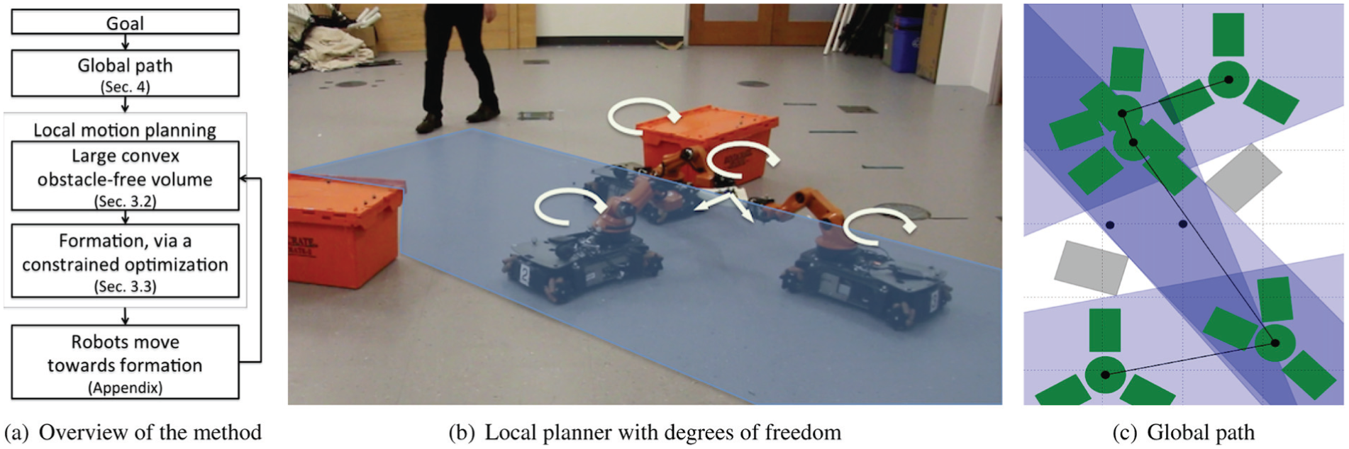
(a) Schematic overview of the method. Given a goal location for the team of robots, we first compute a global path from the start to the goal location, see Section 4. Then, the robots navigate along this path with continuous replanning via a local motion planner, which is described in Section 3. (b) Example with three mobile manipulators collaboratively carrying an object, see Section 5 for the extension of the method to cooperative object transport. In this case, the robots can rotate around their grasping point and a projection of the obstacle-free convex region is shown in blue. (c) Global path to navigate from the formation on the bottom left to the formation on the top right, see Section 4. Obstacles are shown in gray and the robots’ formation in green. Obstacle-free convex regions (blue) connect the start with the goal configuration. Two regions are grown from the start and goal positions and the two intermediate regions are grown from random samples in the workspace (black dots). An optimized formation, in green, was computed for each of the two intersections between adjacent regions. The resulting path (solid black line) connects the start and the goal configurations and traverses through the convex regions.
1.3.2. Global path planning
We also describe a method for global path planning from an initial configuration to a final configuration. The method, see Section 4, computes for the team of robots a path, and a set of safe intermediate formations. The robots avoid static obstacles and reconfigure their formation as required.
Our method presents similarities with sampling-based methods such as the Rapidly-Exploring Random Trees RRT approach by LaValle and Kuffner (2001). There, sampling was performed in configuration space and samples (i.e. configurations) and transitions were collision-checked with respect to obstacles. Here we describe an alternative, where sampling is performed in the low dimensional workspace, transitions between formations are guaranteed via convex polytopes, and safe configurations of the formation are obtained via a constrained optimization. The method introduced in this work explores the non-convex workspace and improves the quality of the solution over time thanks to sampling, while remaining efficient due to the constrained optimization and the use of convex regions, which provide a dimensionality reduction.
We create a graph of feasible formations, which connects the initial with the goal configuration. Each node in the graph is a valid configuration, which corresponds to a feasible formation embedded in free-space. Each edge between two configurations is associated with an obstacle-free convex region embedded in the workspace
In Figure 3(c) we show an example of the method where three mobile manipulators carry an object from a start configuration (bottom left) to a goal configuration (top right). We display the first feasible path found by the algorithm, together with the sampled convex regions and the intermediate formations within the intersections.
1.3.3. Generality
We will first describe, in Sections 3 and 4, the method for a team of mobile robots navigating in a formation that can change shape via isomorphic transformations. We will then, in Section 5, describe an alternative formation definition for mobile manipulators collaboratively carrying objects. The method is general and can be adapted to other high-dimensional problems or formation definitions. The core idea is to generate convex, obstacle-free regions and then optimize the parameters of the formation (i.e. the degrees of freedom of the high-dimensional configuration) such that the robots are fully contained in the convex region. The only requirements to adapt the method are (a) a function
In this paper, we describe two applications.
Formation control: The configuration of the robot team is given by the 3D position, size, and 3D orientation of the formation, i.e.
Collaborative transportation with mobile manipulators: The configuration of the robot team is given by the 2D position and orientation of the object that the robots carry, the orientation of the n robots around their grasping points and the length of their arms, i.e.
An advantage of the method is that planning is decoupled into: (a) finding convex regions in the lower-dimensional free position-time space (
1.3.4. Organization
In Section 2 we introduce the notation and we describe the formation definition and the method to compute convex regions. The algorithm for local motion planning is detailed in Section 3, followed by the global path planner in Section 4. In Section 5 we introduce an extension of the method for transportation of an object by multiple manipulators. Section 6 presents experimental results with mobile manipulators and simulations with aerial vehicles. Finally, Section 7 provides a discussion of the method and Section 8 concludes this paper.
2. Preliminaries
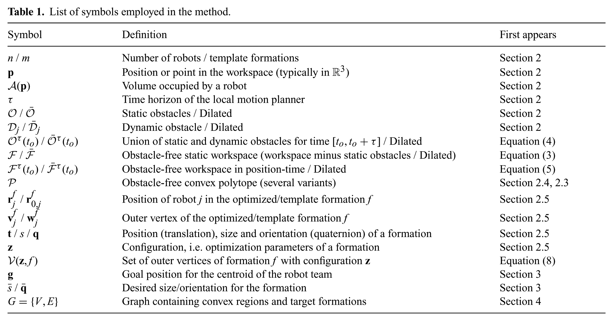
In Table 1 we provide a list of the main symbols and variables employed in this paper.
List of symbols employed in the method.
2.1. Robots
Consider a team of robots navigating in formation. For each robot
For an alternative description of the robots, where cylindrical shape is not required, refer to the extension for rectangular mobile manipulators in Section 5.
2.2. Obstacles
Consider a set of static obstacles

Moving obstacles within the field of view of the robots can be accounted for. Denote by

its dilation by half of robot’s volume. For predicted future positions we employ the constant velocity assumption.
2.3. Obstacle-free workspace
The obstacle-free workspace, accounting only for static obstacles, is denoted by

For current time
where
The position-time obstacle-free workspace is then

2.4. Directed obstacle-free convex region
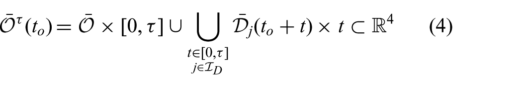
The first building block of the proposed algorithm is to, given an obstacle map and a starting point, compute an obstacle-free convex polytope. We employ a fast iterative method, by Deits and Tedrake (2014), to compute large convex polytopes in free position space, i.e.
Considering a set of points
Growing the region
Example of a convex directed polytope
If the polytope is embedded in position space, we denote by
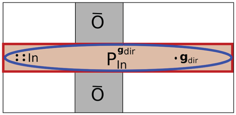
2.5. Definition of the formation
For an alternative description of the formation, refer to the extension for mobile manipulators in Section 5.
We consider a predefined set of
(a) Example of a template square formation with sixteen MAVs. The four outer vertexes define the convex hull. (b) The formation can be transformed with a translation
Further denote by
A formation is then defined by an isomorphic transformation, which includes the size
Given the configuration
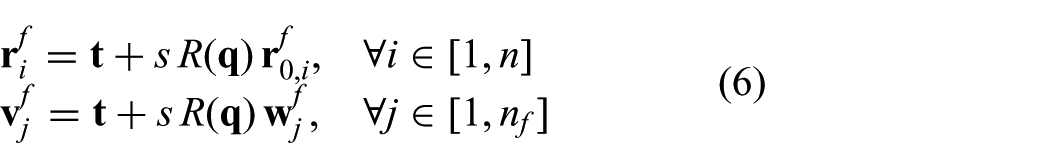
where the rotation in
For template formation f and configuration
In the exposition of the method we rely on this definition for the formation, but the method is general and can be applied to alternative definitions, as shown in Section 5 for the case of several manipulators transporting a rigid object.
3. Local motion planning
The local motion planner computes the optimal parameters, i.e. the configuration, of the formation, in a neighborhood of the robots, via a constrained nonlinear optimization. For a given template formation
Denote by
For an alternative formulation of the optimization, see the extension for mobile manipulators in Section 5.
3.1. Algorithm overview
To make progress towards the goal position while avoiding obstacles, the local planner computes a target formation and the required motion of the robots for a given time horizon
Our method consists of the following steps.
Compute a large convex polytope
Compute the optimal formation
In a faster loop, described in Section 3.5, the robots are optimally assigned to target positions in the formation and move towards them employing a low level local planner that generates collision-free inputs that respect the robot’s dynamics. In particular, we build on a distributed convex optimization described by Alonso–Mora et al. (2015c), extended to account for static obstacles in a seamless way.
If no feasible formation exists in a neighborhood of the robots, we search for the parameters of a target formation near the goal position. In this case, the robot team splits and each robot navigates independently towards its assigned position in the target formation.
3.2. Obstacle-free convex region
First, the obstacle-free space in position-time
For the given time horizon
Following Section 2.4, we compute two convex polytopes.
This polytope may not contain all the robots at their current positions.
A representative example of these regions (projected in

which:
guarantees that the transition to the new formation will be collision-free, since
is likely to make progress in future iterations, since
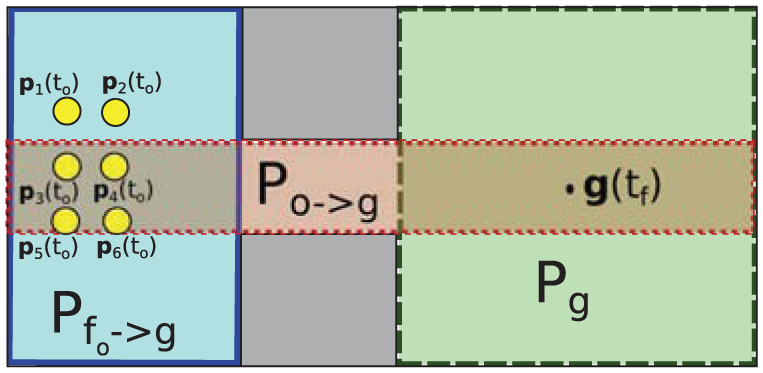
Example of convex regions computed with the method described in Section 2.4 for a scenario with six yellow disk robots and two (gray) squared obstacles. The convex regions are:
Once the robots are within this intersection they can make progress towards the goal within
We rely on a representation of the collision-free convex polytope

where
3.3. Nonlinear optimization
We formulate a constrained nonlinear optimization to compute a locally optimal formation
3.3.1. Optimization cost
We minimize a weighted sum of the deviation with respect to the formation’s goal

where
3.3.2. Constraints
Constraints are introduced to guarantee that all the robots in the formation are within the convex polytope (C1) and to satisfy a minimum inter-robot distance (C2) to avoid collisions between the robots in the team. Recalling Section 2.5 the constraints are then given by
where C1 contains a constraint for each vertex
For planar formations, the additional constraints
3.3.3. Nonlinear program
For a template formation
We employ the nonlinear solver SNOPT by Gill et al. (2002), which internally executes a sparse Sequential Quadratic Program and converges to a feasible local minimum of the cost function.
The derivatives of the cost function (equation (13)) and constraints (equation (14)) are given by

where
We set the initial point for the optimizer to

where the initial quaternion is chosen to be equal to the quaternion addition of the desired orientation and a small random quaternion, i.e.
If the constrained optimization of equation (15) is solved for each template formation, the index
This formation definition and its associated nonlinear optimization are given as an example, but the framework is general and can be applied to other problem instances. In Section 5 we describe how to apply this method for the manipulation of rigid objects.
3.4. Iterations if problem is infeasible
The method, as described in the previous subsections, results in a formation and its configuration for the robots’ team. It may occur though, that the robots make no progress towards the goal (deadlock) or that the optimization is infeasible, for example if the region
First, we would repeat the optimization using the convex region
If this additional step is also unfeasible, then no formation may exist such that the robots can continue navigating in formation towards the goal. In that case the optimization can be repeated using the polytope
3.5. Individual planning towards target formation
The result of the computation of Section 3.3 is a target formation
In this section, we describe the local planner that links the centralized formation optimization with the physical robots. At each step of the execution, at higher frequency than that of computing a new formation, the following steps are executed.
3.5.1. Goal assignment
Robots are optimally assigned to the target positions
Following Alonso–Mora et al. (2012), this assignment can be centrally computed with the optimal Hungarian algorithm by Kuhn (1955), used in this work, or a suboptimal auction algorithm by Bertsekas (1988), which scales well with the number of robots.
3.5.2. Collision avoidance
To control the individual robots in the team and to avoid collisions between them, we employ the collision avoidance algorithm introduced by Alonso–Mora et al. (2015c). We employ the same constraints to avoid moving obstacles and to respect the kinematic model of the robots. To better handle environments with static obstacles, we include additional linear constraints defined by a convex polytope in free space, computed in a neighborhood of the robot. For details refer to the Appendix. This method, a convex optimization in velocity space, is well suited for our application. The formation control algorithms described in this paper are agnostic to the low-level controller and a different one could be employed.
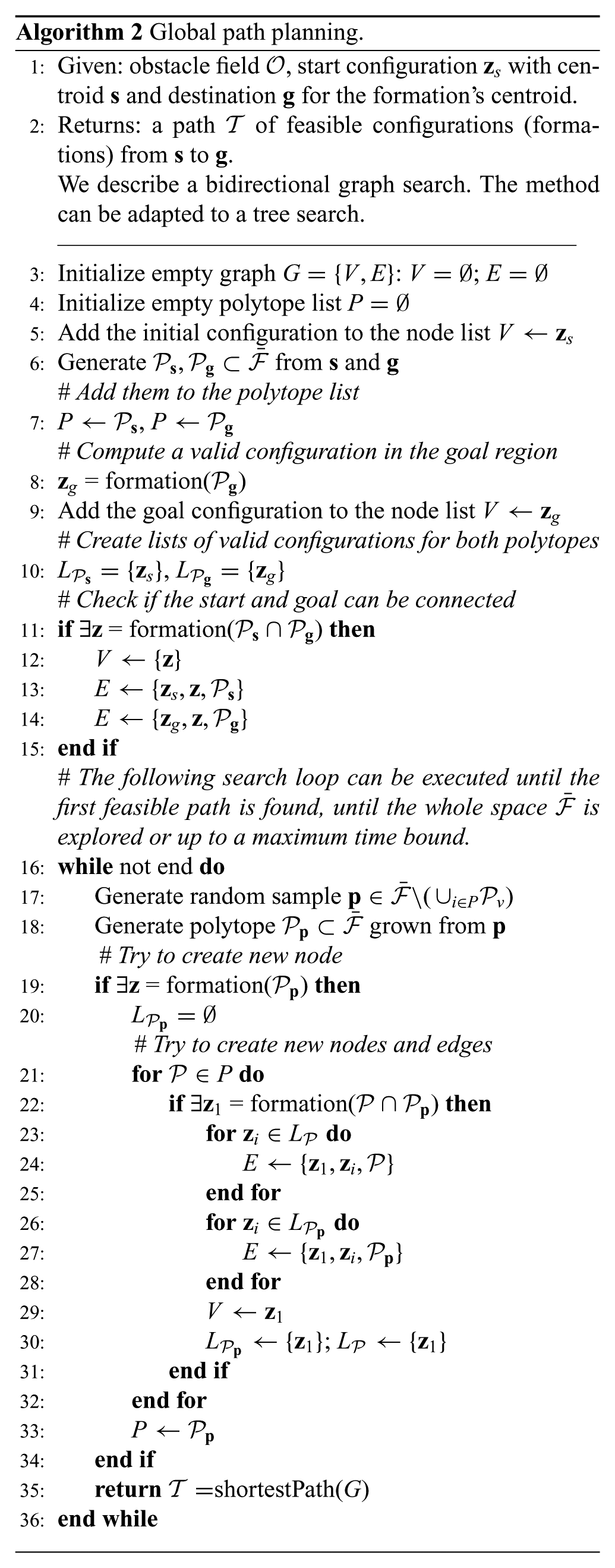
4. Global path planning
Given an initial and a target configuration for the robot team, the global path planner computes a feasible path and intermediate formations to connect them. This is achieved by combining a sampling-based approach with constrained nonlinear optimization, the idea being to sample in a low dimensional space (workspace) and letting the optimizer compute the remaining degrees of freedom.
In particular, we create a graph where each node is a feasible formation and which contains the initial and the goal configuration. An edge between two nodes, or formations, is a convex region in free space, which contains both formations. An edge provides the means to transition between two nodes in the graph. An example was shown in Figure 3(c).
The approach can be applied to a single user-defined formation (i.e. square) or when multiple formations are given. In the latter, reconfiguration between formation shape would be allowed. In an abuse of notation, throughout this section we drop the subindex
4.1. Algorithm
Consider the obstacle-free workspace
A graph
We keep a list of existing polytopes P. And, for each polytope
The method proceeds by drawing random samples in the workspace (
A large convex polytope
For each polytope
If a valid configuration
A feasible solution is found as soon as a path (or sequence of connected vertexes in the graph G) is found which connects the initial position with the goal position of the formation’s centroid. If we let the algorithm run longer, for example until most of the free space is covered by convex regions, the best path so far is found via graph search. This is, by computing the path of lowest cost in the graph G. For each edge E between two configurations
4.2. Execution in composition with the local motion planner
To navigate the team of robots from the initial to the goal configuration a global path consisting of a sequence
To reach the final goal, the team of robots sequentially follows the intermediate setpoints in the path and the local planner minimizes the deviation towards the associated configuration
We do not directly use the convex regions stored in the global path, since the robots need to account for dynamic obstacles in real-time.
First, a convex region
Otherwise, we compute its intersection with a polytope generated with only the centroid of
5. Extension for mobile manipulators
In this section, we describe an extension where a team of mobile manipulators collaboratively carry an object in a dynamic environment. To achieve this, the robot shape, formation definition, and optimization equations are modified, and the derivations follow the same line of thought of the previous sections.
5.1. Robot and formation definition
The formation is defined by n mobile manipulators, each equipped with a robotic arm and grasping a rigid object at given points, see Figure 5(b) for an example with two mobile manipulators.
The position
The vertices of the object relative to its center and expressed in the object coordinate frame are denoted by
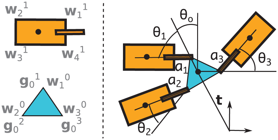
Right: optimization variables for three mobile manipulators grasping a triangular object. Left: vertices of a mobile manipulator and the grasped object. For this triangular object, the vertices are equal to the grasping points.
Given the configuration
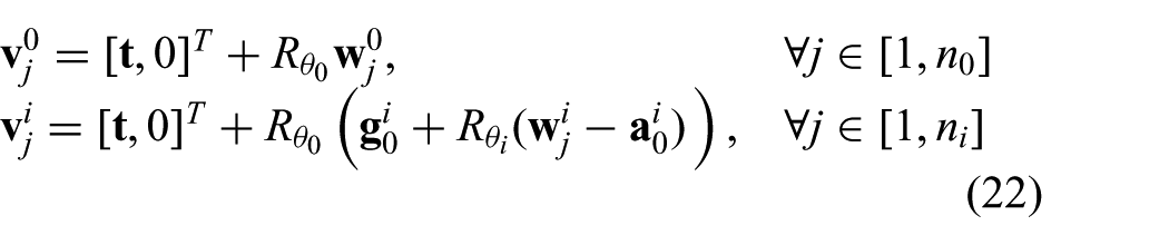
where

the set of
5.2. Obstacle-free convex region
Recalling Section 2.3, the position-time obstacle-free workspace is given by
where, now, the static and dynamic obstacles are not dilated.
The collision-free convex polytope containing the robots at their current state and directed towards the goal is
additional polytopes in free space are computed analogously.
5.3. Nonlinear optimization
Consider
Since the robots are rigidly attached to the object, we must explicitly impose that the transition between the current and the target configuration remains within the convex polytope. Consider
Recalling equation (22) and the representation of the collision-free polytope
The derivatives of the constraints with respect to the optimization variable
6. Results
In this section, we present experiments with a team of three Kuka Youbot mobile manipulators collaboratively carrying an object and simulations with teams of quadrotor UAVs navigating in 3D environments. A video illustrating the results accompanies this paper and is also available at https://youtu.be/sDNqdEPA7pE.
The mobile manipulators are holonomic platforms. For the UAVs, we employ the nonlinear dynamical model and LQR controller used by Alonso–Mora et al. (2015c) with real quadrotors.
We use SNOPT by Gill et al. (2002) to solve the nonlinear program via Sequential Quadratic Programming, a goal-directed version of IRIS by Deits and Tedrake (2014) to compute the large convex regions and the Drake toolbox 3 from MIT to handle quaternions.
6.1. Multiple aerial vehicles in formation
To evaluate our approach in 3D environments with aerial vehicles we present experiments in three simulated scenarios. The first scenario consists of four controlled quadrotors and four dynamic obstacles. The second scenario consists of four controlled quadrotors flying in formation and avoiding several static obstacles and one dynamic obstacle. The last scenario involves sixteen quadrotors flying in formation through a narrow corridor. In our visualizations, we employ a cylinder since that is the shape we use for collision avoidance. Internally the quadrotors have an attitude controller and position controller and change their 3D pose within the enclosing cylinder, which is always kept vertical.
In all cases a new formation is computed every 2 s. The individual collision avoidance planners run at 5 Hz. The quadrotors move at speeds between 0.5 m/s and 1.5 m/s. In our simulations with four quadrotors a time horizon
Consider the first scenario. Figure 8 shows the trajectories of four quadrotors (in green and blue) passing through two lanes of dynamic obstacles (in yellow). The dynamic obstacles in the left lane move downwards at 0.4 m/s and the ones in the right move upwards with the same speed. Two default formations are considered, square (which is preferred) and diamond. The goal for the formation follows a constant velocity trajectory along the middle horizontal line and the team successfully adapts the parameters of the formation to remain collision-free and pass in-between the obstacles. In this case, we imposed that the formation remains on the horizontal plane for illustrative purposes.
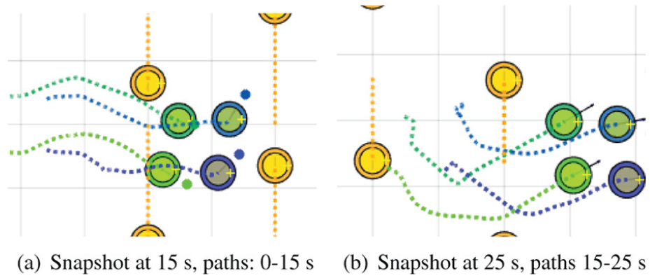
Top view. Four robots (green-blue) navigate a 8 x 15 m2 environment with two lanes of dynamic obstacles (orange). The four robots locally reconfigure the formation and make progress towards the right side.
In order to evaluate the robustness of the method, we performed additional experiments for this first scenario for varying speeds of the dynamic obstacles and the quadrotors flying in formation. The results are presented in Figure 9. We observe that most of the time the target formation for the robots is within
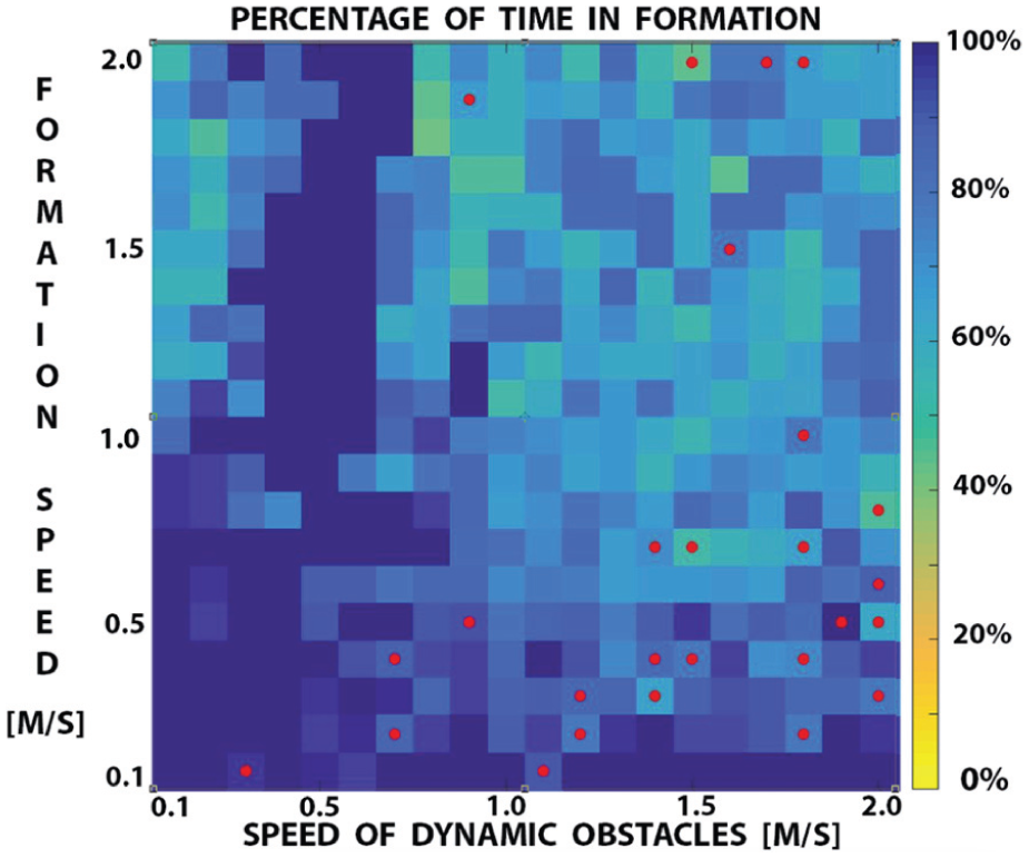
Results for 3D navigation in the scenario of Figure 8 with four quadrotors and varying speeds of the dynamic obstacles and the formation. Fixed time horizon of
In this scenario, very few collisions arise when the target speed of the formation is higher or similar to that of the dynamic obstacles and our framework successfully drives the robots towards the goal while avoiding collisions. Some collisions arise when the speed of the dynamic obstacles is much higher than that of the formation. This is due to the local planning horizon and the robots being unable to escape on time due to their lower speed. Again, these results may be improved with an adaptive time horizon of the framework.
Next, we present experiments for the second scenario. Figure 10 shows snapshots and trajectories of four quadrotors tracking a circular trajectory while locally avoiding three static obstacles and a dynamic obstacle. Three default formations are considered here: square (1st preference), diamond (2nd preference), and line. The optimal parameters are computed with the nonlinear optimization allowing rotation in 3D (flat horizontal orientation preferred) and reconfiguration.
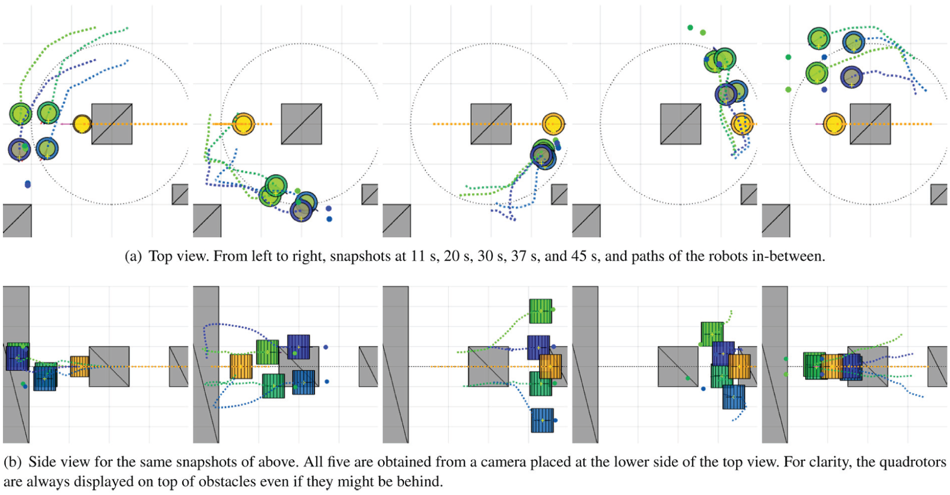
Four quadrotors (green-blue cylinders) navigate in a 12 x 12 x 6 m3 scenario with three static obstacles (grey) and a dynamic obstacle (yellow). The four quadrotors track a circular motion (black dots in top view) and locally reconfigure the formation to avoid collisions and make progress.
The four quadrotors start from the horizontal square and slightly tilt it (11 s) to avoid the incoming dynamic obstacle. To fully clear it while avoiding the obstacle in the lower corner, they shortly switch to a vertical line, and then back to the preferred square formation (20 s). To pass through the next narrow opening they switch back to the line formation (30 s) and then to the preferred square, tilted to avoid the dynamic obstacle (37 s). Once the obstacles are cleared they return to the preferred horizontal square formation (45 s).
Results of the third scenario, where sixteen quadrotors move along a corridor of three different widths are shown in Figure 11. Three default formations are considered: 4x4x1 defined by four vertices (preferred), 4x2x2 defined by eight vertices and 8x2x1 defined by four vertices. At each time step the method computes the optimal parameters for each of the three and selects the one of lowest cost. Between times 75 s and 110 s the method successfully rotates the formation by
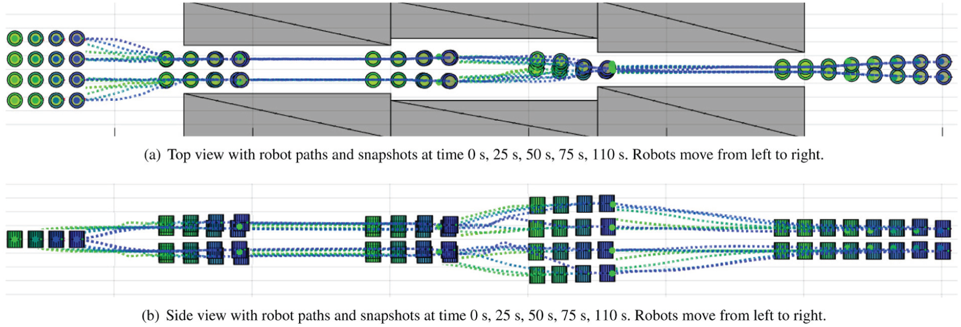
16 quadrotors navigate along a 70 x 10 x 10 m corridor, with obstacles shown in gray. The quadrotors locally adapt the formation to remain collision free. The following formations are observed: 4x4x1 - 4x2x2 - 4x4x1 (vertical) - 8x2x1 (vertical), finally transitioning towards horizontal 8x2x1.
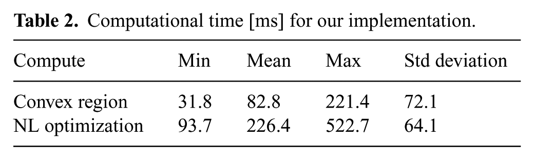
Thanks to the abstraction of a formation by the vertices of its convex hull, see Section 2.5, the computation time of the nonlinear optimization is independent of the number of robots - as long as the same convex shape is maintained - and can be executed in real-time. It is worth noting that in this algorithm the dimension of the space where the robots move has little influence in the computational cost, which depends mostly on the number of variables defining the formation. In Table 2 we provide computational times for our implementation using a 2.6 GHz i7 laptop. The approach shows close to real time performance, typically below 300 milliseconds
Computational time [ms] for our implementation.
6.2. Collaborative transport with two mobilemanipulators
We performed initial experiments with two mobile manipulators carrying a rigid object, as described in Section 5. In this first experiment the two robots are not allowed to change their orientation and distance with respect to the object (
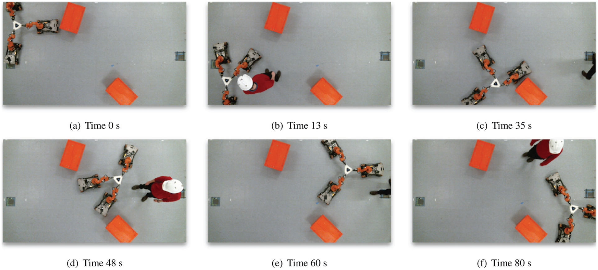
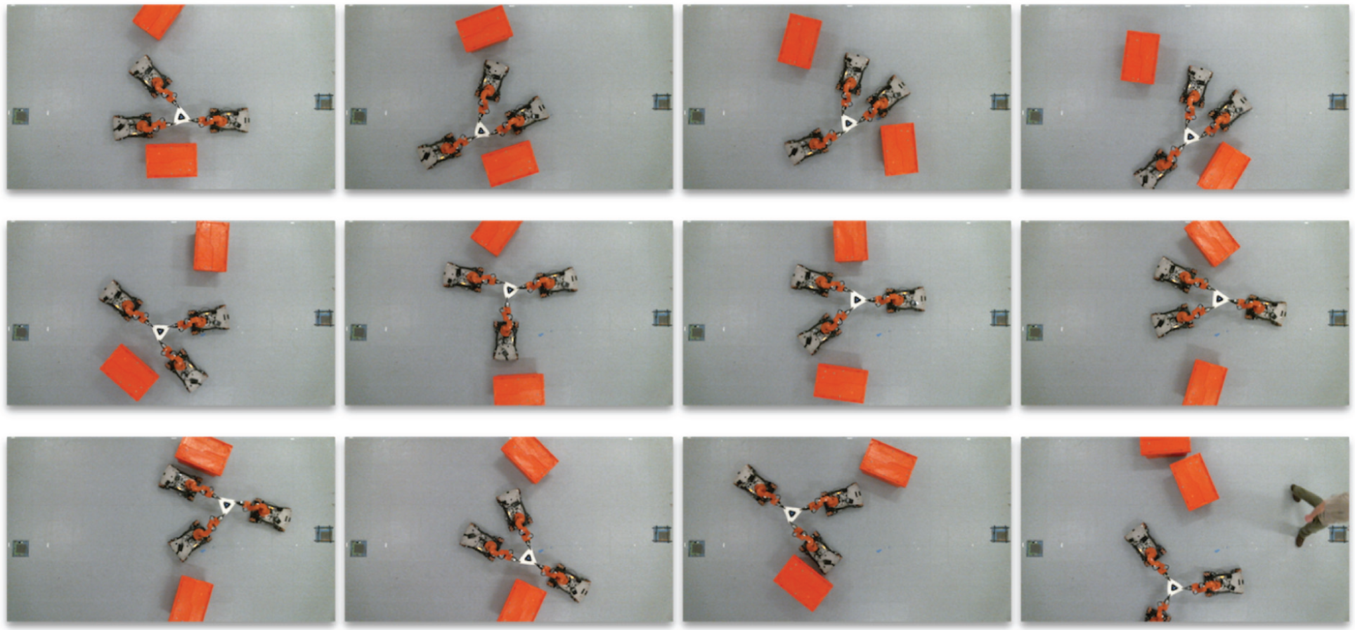
Four snapshots are shown in Figure 12 of an experiment where the two mobile manipulators successfully carry the rigid object to the goal position behind the orange boxes while locally avoiding collisions with the human. In all our experiments, executed with external tracking, the robots successfully adapted their formation to avoid collisions. This assumes that the human cooperates, otherwise, collisions may still occur if the human moves faster than the robots or traps them against an obstacle.
Four consecutive snapshots of an avoidance maneuver where two mobile manipulators collaboratively carry a rigid object and navigate it to the goal while adjusting their formation to avoid collisions with the orange boxes and the human. Robots and human are tracked by overhead cameras. This maneuver is performed in 1 minute.
A visualization with convex regions of another experiment is shown In Figure 13. For each snapshot the current (blue) and target (green) formation given by the optimization are displayed. The two robots successfully adapt their formation, rotating as required, to avoid both the dynamic obstacle (red) and static (grey) obstacles in this 8 m x 6 m scenario. Slices at
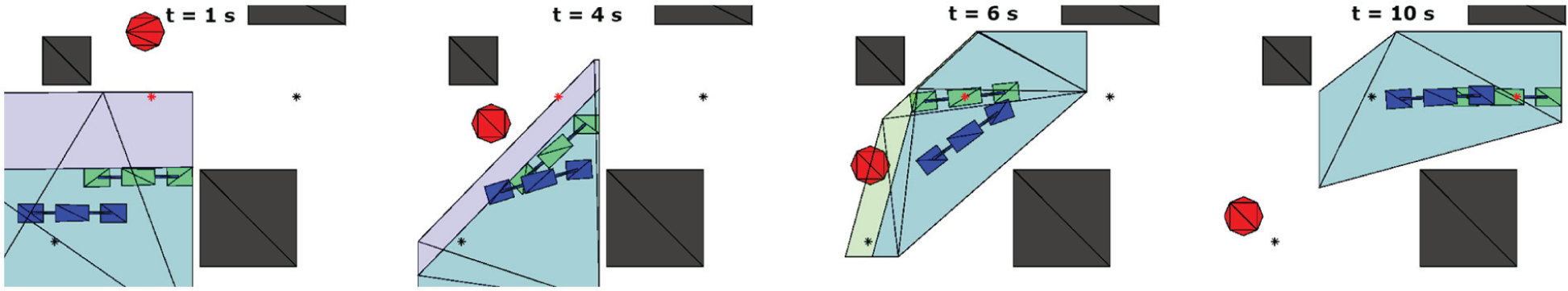
Four consecutive snapshots of a 10 s avoidance maneuver where two mobile manipulators collaboratively carry a rigid object and navigate to two goals (crosses) while avoiding collisions with static (gray) and dynamic (red hexagon) obstacles. The current state of the two manipulators and the rigid object is displayed in blue and the target one (given by the optimization) in green. Two slices of the convex polytope are shown, purple for the current time
6.3. Collaborative transport, three mobilemanipulators
We performed additional experiments with three mobile manipulators carrying an object, as described in Section 5. All three robots can change their orientation respect to the object, but their distance remains constant. We optimize for the position and orientation of the object and the orientation of all three manipulators. Given a goal for the formation, we first compute a global path with the algorithm of Section 4 considering only the two static obstacles. The local motion planner then runs at a frequency of approximately 5 Hz, accounts for the dynamic obstacle (person), and updates the parameters of the formation. A low-level controller is employed which, via high-frequency interpolation, drives the robots towards the desired formation.
We tested different configurations of the two boxes in our experimental space, covering all possible scenarios we thought of (some examples are shown in Figure 14). In all our experiments the robots could avoid collisions and reach the goal - as long as the human moved at a reasonable speed below that of the robots and did not aggressively push them against a wall.
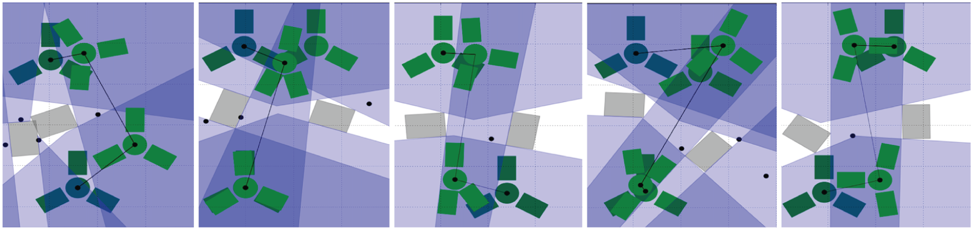
Five examples of the global path planner for different scenarios with two static obstacles. The three mobile manipulators carry an object and can rotate and translate while grasping. The initial and final formations are displayed in dark green. Light green formations are additional nodes of the graph. The first feasible path is displayed with a solid black line. All samples (black dots), polytopes (blue) and optimized formations (green) within the intersections of polytopes are shown. Typically, a feasible path is found with very few samples.
Several configurations of the two boxes, with the computed global path, are shown in Figure 14. All of them were computed in the order of below ten seconds. The initial configuration is in the lower part of the images and the goal configuration in the upper part. In each figure, we display the samples (black dots), the convex regions (blue), the optimal formations within each intersection (green) and the path. We stop the construction of the graph as soon as the first solution is found. We observe that in general, very few iterations were required to find a feasible solution, which is also of good quality thanks to the optimizer. Navigation in all these scenarios was successfully achieved by the three mobile manipulators.
A representative experiment where the three robots navigate through the boxes and avoid a human is shown in Figure 15. For reference, in Figure 16 we show twelve different scenarios and the configuration of the three robots when navigating through the environment.
Three mobile manipulators collaboratively carry an object and navigate to a goal position in the other side of the room. The global path planner guides them through the two static obstacles and they locally avoid the walking human. The robots successfully adapt their formation to pass through the narrow opening and avoid the human.
Twelve different experiments where the three mobile manipulators collaboratively carry an object and navigate to a goal position in the other side of the room. For each one of them, a snapshot while they traverse through the two obstacles is shown. This experiment shows robustness to the location of the obstacles and that the robot formations vary across different execution runs. If the obstacles leave enough free space, as is the case in the lower right corner experiment, the team of robots maintain the preferred formation and do not need to rotate around their grasping points. Otherwise, they successfully adapt the configuration.
In these experiments, we employed a triangular object with foam exterior. The foam provides a small degree of deformability to compensate for the lack of compliance in the robot arms and low level controller of the mobile manipulators. Note that successful manipulation of a perfectly rigid body was shown in the previous experiments with two mobile manipulators, albeit at lower speeds.
6.4. Global planning in large scenarios
We also tested the approach in several larger scenarios. In Figure 17 we show two examples of the global planner in simulated 2D environments. In these two cases the global planner can run for several iterations, up to a fixed amount of time. We display all the computed convex regions and formations. After finding the first feasible path connecting the start with the goal position, we store (and display) the subsequent shorter paths found by the algorithm. An advantage of the method is that large areas in free space are explored by each convex polytope, which reduces the need for additional samples within.
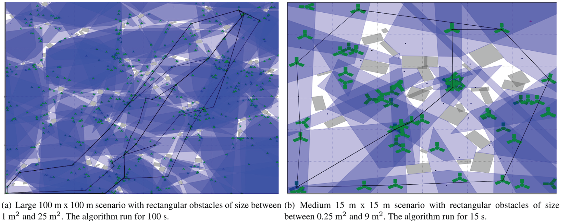
Two examples of the global path planner connecting a start (lower left corner) with a goal (upper right corner) for two large scenarios with many static obstacles. The three mobile manipulators carry an object and can rotate and translate while grasping. The algorithm runs for a fixed amount of time. The first feasible path, and the feasible paths found in subsequent iterations that decrease the cost, are displayed with a solid black line. All samples (black dots), polytopes (blue), and optimized formations (green) within the intersections of polytopes are shown.
7. Discussion
The method described in this paper showed good real-time performance and could successfully compute the optimal parameters for the multi-robot formation, while allowing for reconfiguration. The method provided collision-free navigation among static and dynamic obstacles in simulations with aerial vehicles and in experiments with mobile manipulators.
At least in part, the computational efficiency and the good scalability with respect to the number of robots in the formation is achieved by (a) not including the agent dynamics in the formation optimization but handling them in the individual local planners (this works well for robots with fast dynamics); and (b) considering the convex hull of the formation. In fact, the number of variables and constraints of the formation. In fact, the number of variables and constraints of the formation control method is independent from the number of robots. The optimization problem in Equation (15) has eight variables for 3D motion and
In our experiments, the computation of a large obstacle-free convex polytope following Section 2.4 showed very good results, but no guarantees exist that the best volume will be obtained. In fact, the method will converge to a local optimum of the cost function, which is guaranteed to be fully contained in free space. Searching over several regions might prove advantageous. One may also consider employing a faster, albeit suboptimal algorithm to quickly compute a convex region.
To compute the parameters of the multi-robot formation our method solves a nonlinear optimization via Sequential Convex Programming. This method converges to a local optimum of the non-convex problem. Global optimality can only be guaranteed if the original optimization problem is convex, which is typically not the case. For the non-convex case, the number of iterations required to find a locally optimal, or even feasible, solution is not defined. In practice, the method performed very well, quickly returning good parameters for the formation in all cases where a valid formation could be fitted within the convex polytope.
These observations also apply to the case of the global planner and no strong guarantees can be given for the general non-convex optimization case. Thanks to the sampling of convex regions, the method will successfully explore the whole workspace. For speed-up, as described in Algorithm 2, we limit the sampling of regions to points outside of the union of current convex regions in the graph. In most scenarios this heuristic works well, but it can potentially miss narrow openings, since, although the whole space is covered by convex regions, the intersection might not be traversable. Two advantages of this method are (a) that sampling is performed in a low dimension space - the workspace - instead of in the high-dimensional configuration space and (b) that large areas of the free space are explored/covered at once when contained within a convex polytope. This has the potential to speed-up global path planning for formations of robots.
If the optimizations are feasible and a solution is found, the motion is guaranteed to be collision-free up to the time horizon of the local planner, under the assumption that the moving obstacles maintain a constant speed. This is true because: (a) the convex region is fully contained in free position-time space; (b) the robots at their initial position and at the positions in the target formation are fully contained in the convex region and (c) the motion in between the two formations as well, if the robots move in a straight line (the linear combination of two points lies within the convex polytope). For mobile manipulators collaboratively carrying an object, this is satisfied up to the interpolation.
Nonetheless, collisions with moving obstacles can still arise if the assumptions are not met. For instance, if the moving obstacles change the direction of motion quicker than the robots can react, if the moving obstacles move too fast, if the planning horizon is not long enough, or if the team of robots are trapped in a corner from where they cannot feasibly escape.
An advantage of the method is that planning is decoupled into: (a) finding convex regions in the lower dimensional free position-time space (
Lastly, the method is general and can be adapted to other high-dimensional problems or formation definitions. The core idea of the algorithms is to generate convex obstacle-free regions and then optimize the parameters of the formation (i.e. the degrees of freedom of the high-dimensional configuration) such that the robots are fully contained in the convex region. The only requirements to adapt the method are (a) a function that converts configurations
8. Conclusion
In this paper, we showed that navigation of teams of robots in formation among arbitrary static and dynamic obstacles can be achieved via a constrained nonlinear optimization. By first computing a large obstacle-free convex polytope and then optimizing the formation parameters, low computational cost is achieved together with good navigation results. In several simulations with aerial vehicles navigating in 3D environments we showed successful navigation in formation where robots may reconfigure the formation as required to avoid collisions and make progress.
Our method can be applied both for real-time local navigation in a dynamic environment and to compute global paths in static environments. The global planner successfully combines a sampling-based method in the workspace with nonlinear optimization for the remaining degrees of freedom of the formation, thus reducing the dimensionality of the sampling problem.
For formation control, the approach scales to teams of robots of arbitrary size, since only the convex hull of the formation is employed in the constrained optimization. Simulations with sixteen quadrotors -although more could be used - demonstrate this. The approach is general and can also be adapted to other formation definitions and applications, as showed in our experiments with three mobile manipulators collaboratively carrying an object,
In this work, we did allow for splitting and merging of robots, from/to a joint formation to/from individual navigation. An interesting avenue for future work is that of splitting and merging of the group formation into smaller sub-formations, or to maintain the formation while letting dynamic obstacles through, which is currently not possible. Additional avenues of future research include incorporating the dynamic constraints of the robots in the nonlinear optimization problem and accounting for uncertainties in the prediction of the movement of the dynamic obstacles. In this work, the nonlinear dynamics of the robots were decoupled from the formation control and accounted for by the individual controllers locally.
Footnotes
Appendix: Collision avoidance
In this appendix, we provide a description of the method for collision avoidance employed with the aerial vehicles. We implement the convex optimization introduced by Alonso–Mora et al. (2015c) with identical motion constraints and constraints for avoidance of other agents. This approach adapts to changes in the environment, avoids moving obstacles, and respects the dynamics of the robot via a set of motion primitives. Each motion primitive was defined to track a constant reference velocity with a robot-specific controller.
We extend the method towards environments with complex static obstacles. In particular, using the convex polytope computation described in Section 2.4, we add a new constraint to guarantee that the motion of the robot is within the obstacle-free workspace
Denote by
In Alonso–Mora et al. (2015c) the collision avoidance algorithm was formulated as a constrained optimization in
velocity space. Therefore, the convex region needs to be converted to an equivalent region in velocity space. Given the time horizon
where each linear constraint defining
If the target position
Acknowledgements
The authors are grateful to Robin Deits and Hongkai Dai from MIT for their help with IRIS, Drake and SNOPT.
Funding
This work was supported in part by the MIT Lincoln Laboratory, SMARTS N00014-09-1051, pDOT ONR N00014-12-1-1000 and the Boeing Company.