Sage Journals: Discover world-class research

Abstract

Background

In microsimulation models of diseases with an early, acute phase requiring short cycle lengths followed by a chronic phase, fixed short cycles may lead to computational inefficiency. Examples include epidemic or resource constraint models with early short cycles where long-term economic consequences are of interest for individuals surviving the epidemic or ultimately obtaining the resource. In this article, we demonstrate methods to improve efficiency in such scenarios. Furthermore, we show that care must be taken when applying these methods to epidemic or resource constraint models to avoid bias.

Methods

To demonstrate efficiency, we compared the model runtime among 3 versions of a microsimulation model: with short fixed cycles for all states (FCL), with dynamic cycle length (DCL) defined locally for each state, and with DCL features plus a discrete-event-like hybrid component. To demonstrate bias mitigation, we compared discounted lifetime costs for 3 versions of a resource constraint model: with a fixed horizon where simulation stops, with a fixed entry horizon beyond which new individuals could not enter the model, and with a fixed entry horizon plus a mechanism to maintain a constant level of competition for the resource after the horizon.

Results

The 3 versions of the microsimulation model had average runtimes of 515 (95% credible interval [CI]: 477 to 545; FCL), 2.70 (95% CI: 1.48 to 2.92; DCL), and 1.45 (95% CI: 1.26 to 2.61; DCL-pseudo discrete event simulation) seconds, respectively. The first 2 resource constraint versions underestimated costs relative to the constant competition version: $20,055 (95% CI: $19,000 to $21,120), $27,030 (95% CI: $24,680 to $29,412), and $33,424 (95% CI: $27,510 to $44,484), respectively.

Limitations

The magnitude of improvements in efficiency and reduction in bias may be model specific.

Conclusion

Changing time representation in microsimulation may offer computational advantages.

Highlights

Short cycle lengths may be required to model the acute phase of an illness but lead to computational inefficiency in a subsequent chronic phase in microsimulation models.

A solution is to create state-specific cycle lengths so that cycle lengths change dynamically as the simulation progresses.

Computational efficiency can be enhanced further by using a hybrid model containing discrete-event-simulation-like features.

Hybrid models can efficiently handle events subsequent to exit from an epidemic or resource constraint model provided steps are taken to mitigate potential bias.

Keywords

microsimulation discrete event simulation hybrid models open parallel models computational efficiency

Individual-level simulation overcomes the constraints of Markov cohort models by allowing individual heterogeneity and memory of prior events (see the supplemental appendix for details on these and other simulation methods discussed below).¹ Two common simulation structures include microsimulation and discrete event simulation (DES).^2,3 The latter is computationally more efficient than microsimulation.³ Further, since DES measures elapsed time continuously, it avoids the positive or negative model output biases that occur due to accounting of health state membership at either the beginning or end, respectively, of discrete time steps (cycles).^4,5 Nonetheless, an analyst may wish to retain the microsimulation structure, particularly in infectious disease and resource constraint models where simulated individuals interact with each other. In such parallel microsimulation models, it may be convenient to keep individuals synchronized with respect to time by having the simulation proceed forward in discrete cycles of uniform duration.

We define a fixed cycle length (FCL) microsimulation model as one in which cycle lengths are unchanging, are of uniform duration, and apply globally to all states in the model. An issue arises when an FCL microsimulation models an illness with an early, acute phase, followed by a longer, chronic phase. In the acute phase, events may occur rapidly, necessitating a short cycle length to ensure sufficient granularity, but that then require a large number of cycles within the chronic phase to reach a simulation terminus (an absorbing state, such as death, or a model horizon). Often, the chronic state is quasi-absorbing where the only modeled events are either remaining in the state or being absorbed. The average number of cycles accumulated between the start of a simulation and termination is one factor that determines microsimulation runtime. FCL microsimulation models with short cycle lengths may require a large number of cycles to be spent in a quasi-absorbing state, which may therefore require long runtimes and reduce computational efficiency. Yet efficiency is important for tasks that require the model to be run many times, such as in the context of a 2-dimensional simulation, model calibration, or value-of-information analyses (supplemental appendix).

In this article, we focus on the concept of changing the way time is represented during the course of a microsimulation run. At its simplest, in a model structure we define as dynamic cycle length (DCL), this can be achieved by defining cycle length locally for each health state rather than globally for the entire model. DCL models offer the ability to encompass the granularity required for an acute, early phase of an illness by employing short cycle lengths in those states while avoiding the computational inefficiency of chronic and/or quasi-absorbing states by specifying longer cycle lengths for them. A further boost in computational efficiency may be realized by designing hybrid models that consist of regular microsimulation structure but also have elements that behave like DES model elements. We refer to the latter as pseudo-DES (pDES) components. Rather than having individuals remain in a DCL quasi-absorbing state, albeit with fewer cycles than an FCL model, the analyst samples time to absorption from a distribution. The latter allows the estimation of time from entry into the quasi-absorbing state until absorption to require only a single computational step. Hereafter, we refer to these as DCL-pDES models. In essence, DCL versus FCL is a quantitative change in the way time is represented in a microsimulation model, while DCL-pDES versus DCL is a qualitative change.

Often, microsimulation models simulate a set number of individuals who each enter the model at the simulation origin and are run through the model structure one at a time (i.e., a closed, serial, microsimulation model). Changing time representation using pDES components may be of particular salience in another type of microsimulation structure: open, parallel microsimulation models. These allow new individuals to enter the model after the simulation origin and have individuals running through the model together, in parallel. Examples include epidemic models and resource constraint models in which individuals interact with one another by infecting or being infected by others or competing for scarce resources with others. It may be convenient to represent time in such models with cycles of uniform and often short duration to keep individuals in the model synchronized in time with respect to their interactions.

Typically, open parallel models run over a fixed time horizon, and the model outputs of interest are the rapidity of growth and peak size of the epidemic in infectious disease models or the mean wait time and wait-list size in resource constraint models, rather than health economic outputs such as quality-adjusted life expectancy (QALE) or costs. However, analysts may wish to explore the long-term health economic consequences of having lived through an epidemic or having to wait for a needed resource. Lifetime horizons are often favored for health economic evaluations, but open, parallel models often require cycles of short duration. This tension is similar to the conundrum described above. Having individuals who survive the epidemic or obtain the constrained resource enter a pDES component with a single transition to the absorbing state may serve as a solution.

A Hybrid Structure for Open, Parallel Models

Incorporating a pDES component addresses the efficiency of open models but creates an issue with horizons. An open model requires a fixed time horizon, since new individuals may enter the model on every cycle and, without the horizon, the model would continue to run indefinitely. A stopping rule based on a maximum number of simulated individuals is often infeasible because the number of new individuals entering the model on each cycle may be stochastic, and the ultimate number of simulated individuals is unknown a priori. With incorporation of a pDES component, a conflict arises between the horizon of the open model and that of the individuals traversing it. With a fixed exit horizon, after which the simulation stops running, individuals entering the model later in the course of the simulation may be trapped in the open, parallel portion and be precluded from accruing long-term quality-adjusted life-years (QALYs) and costs. The latter quantities would therefore be underestimated and biased. A fixed entry horizon, after which new individuals would be prevented from entering the simulated cohort, would allow all individuals who entered the model prior to the entry horizon the potential to accrue long-term costs and benefits. However, individuals entering the model late in the entry window would face an unrealistically low degree of interaction (infection risk or resource competition) after the entry horizon due to the declining size of the active simulated cohort, again leading to bias.

We propose using a fixed entry horizon but include a modification: prior to the entry horizon, new “evaluated” individuals enter the model with each cycle, but after the horizon, only phantoms enter the model. We define a phantom as an individual who may transmit an infection to or compete for a resource with an evaluated individual but does not contribute to the cumulative costs or QALYs generated by the evaluated individuals (those who entered the model prior to the entry horizon). The model runs until the last of the evaluated individuals have been absorbed. This modification specifies a termination criterion for the open, parallel model; allows all evaluated individuals who enter the model late in the simulation the potential opportunity to experience long-term outcomes and ensures that evaluated individuals encounter the same infectious risk or resource constraint after the entry horizon as that which existed prior to the horizon. This setup assumes that the economic interest is of individuals who survived the open, parallel portion of the model from the start of the simulation until the entry horizon; therefore, the contribution of the phantoms to costs and QALE are not considered.

In the remainder of this article, we demonstrate the execution and consequences of altering time representation in microsimulation via a set of example models (FCL, DCL, and DCL-pDES) of hospital discharge run in series. Our first objective was to compare model output and computational efficiency of these 3 structures. Likewise, we addressed the time horizon problem in an economic evaluation of an open, parallel, microsimulation model of surgical wait time. Our second objective was to estimate the reduction of bias between fixed exit, fixed entry, and fixed entry with phantom-based models.

Methods

An FCL Model

We constructed a 2-strategy, 4-state, hospital discharge FCL microsimulation model with a cycle length of 1 d (Figure 1A⁶). The model versions presented here were run in series. Individuals began the simulation admitted to a hospital ward. During a cycle they may have transferred to a rehabilitation facility and then, in a subsequent cycle, they may have been discharged home. From the “Ward,”“Rehab,” and “Home” states, individuals may have transitioned into the “Dead” absorbing state. For simplicity, the model did not include back-transitions, and it considered only health benefits and not costs. Health benefit was expressed for individuals as quality-adjusted lifespan denominated in QALYs, which, when averaged over individuals, yielded QALE.

Figure 1

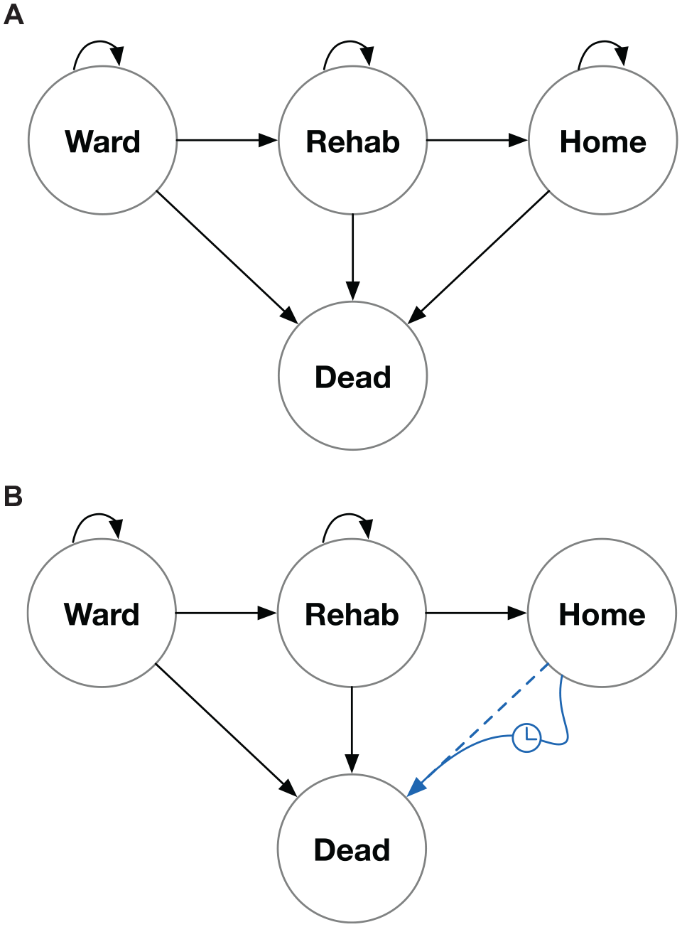
The example model used to demonstrate gains in efficiency for dynamic cycle length (DCL) and hybrid model structures (DCL plus pseudo-discrete event simulation elements [DCL-pDES]) relative to a fixed cycle length (FCL) structure. (A) Structure for FCL and DCL models, in which for the former, cycle lengths are the same for all nonabsorbing states while in the latter, cycle lengths have values that are local to each nonabsorbing state. (B) Structure for the DCL-pDES model. Absorption from the “Home” state is modeled as a single step whose duration is sampled from a Gompertz distribution.

For this illustration, we assumed that input data would come from sources that use different time scales as often happens in modeling practice. For example, probabilities of short-term outcomes (e.g., discharge from hospital) could be based on a short time period (e.g., per day), while long-term outcomes (e.g., death while living in the community) could be based on longer time periods (e.g., per year). Further, we assumed that data existed for the direct observation of pairwise health state transitions within the acute phase of the model (in the “Ward” and “Rehab” states) to which parametric Weibull, time-to-event distributions denominated in days had been fit. We discuss alternative input data structures, particularly systems of differential equations, in the supplemental appendix.

The probability of transition from state i to state j during the course of a cycle was calculated as

P {(t_{D})}_{i j} = 1 - e x p [λ (t_{D}^{γ} - {(t_{D} + δ_{D})}^{γ})]

(1)

where λ and γ were the Weibull scale and shape parameters, respectively, for the transition from state i to j, t_D was the elapsed model time in days, and δ_D was the common cycle length also denominated in days. We provide derivations of this expression and the others below in the supplemental appendix.

For convenience, we used a Gompertz distribution⁷ derived from 50-y-old individuals in the population of Ontario, Canada,⁸ denominated in years, to model absorption from the long-term “Home” state. The per-cycle probability of absorption was calculated as

P (t_{Y}) = 1 - \exp {\frac{λ}{γ} [\exp (γ t_{Y}) - \exp (γ (t_{Y} + δ_{Y}))]}

(2)

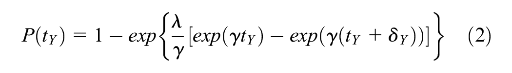
where λ and γ are the Gompertz scale and shape parameters, respectively, derived from Resende et al.,⁸t_Y is the elapsed time in years, and δ_Y is the common cycle length also denominated in years. For the sake of exposition, we made the simplifying assumption that once individuals entered the “Home” state, they faced the same mortality risk as the general population. For the hospital discharge example model, δ_D equaled 1 d and δ_Y equaled 1/365.25 y. We chose Weibull and Gompertz distributions for convenience and note that similar equations for the per-cycle probability of events can be written for other time-to-event distributions.

We employed δ_Y to compute the number of QALYs accrued by an individual inhabiting a state for 1 cycle. QALYs gained for a cycle spent in state i by an individual at t years elapsed was calculated according to the within-cycle correction principle^4,5 as

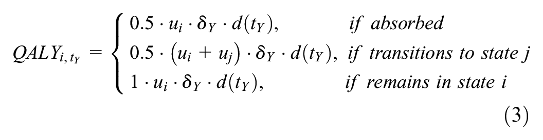
QAL Y_{i, t_{Y}} = {\begin{matrix} 0.5 \cdot u_{i} \cdot δ_{Y} \cdot d (t_{Y}), if absorbed \\ 0.5 \cdot (u_{i} + u_{j}) \cdot δ_{Y} \cdot d (t_{Y}), if transitions to state j \\ 1 \cdot u_{i} \cdot δ_{Y} \cdot d (t_{Y}), if remains in state i \end{matrix}

(3)

where QALY_i,tY was the number of QALYs accrued by an individual starting a cycle in state i at elapsed years, t_Y, and either being absorbed, transitioning to state j, or remaining in state i by the end of the cycle; u_i and u_j were the utility weights for time spent in states i and j, respectively; and d(t_Y) was the discrete discounting function. The latter was defined as

d (t_{Y}) = {(1 + r)}^{- t_{Y}}

(4)

where r was the annual discrete discounting rate (0.015 in Canada according to Canada’s Drug Agency guidelines⁹). For cost-utility analyses, similar expressions could have been used to calculate incremental costs.

We modeled 2 hypothetical strategies, 1 and 2, where the lambda parameter of the Gompertz distribution was reduced by 25% for strategy 2. This is unlikely to represent a realistic intervention, but we used it purely for illustrative purposes to produce a spread in the model output for the 2 strategies.

DCL and DCL-pDES Models

For the DCL version of our hospital discharge example model, we made 2 fundamental changes to the FCL structure. First, rather than specifying a common cycle length, whether denominated in days or years, we defined a local cycle length for each state in the model: for the “Ward” state, δ_D,W = 1 d and δ_Y,W = 1/365.25 y, for the “Rehab” state, δ_D,R = 14 d and δ_Y,R = 14/365.25 y, and for the “Home” state, δ_D,H = 365.25 d and δ_Y,H = 1 y. For the DCL version, these local cycle length values denominated in years replaced δ_Y in the incremental utility expression as defined in (3) above. Second, elapsed time in the model for an individual denominated in years, t_E,Y, was no longer a simple multiple of the number of elapsed cycles. Rather, for a sojourn of 1 cycle in state i during the kth cycle of the simulation, the years elapsed for an individual was calculated as

t_{E, Y, k} = t_{E, Y, k - 1} + δ_{Y, i}

(5)

with a similar expression for elapsed time denominated in days. Elapsed time in years t_E,Y,k replaced t_Y in the discounting function as defined in (4) above.

To improve efficiency further, we developed a hybrid, DCL-pDES version (Figure 1B). Rather than repeatedly cycling through the quasi-absorbing “Home” state, we sampled a time to absorption, t_abs, denominated in years from a Gompertz distribution with the same λ and γ parameters as in the original DCL version. We calculated QALYs gained in the quasi-absorbing state, iu_H, as

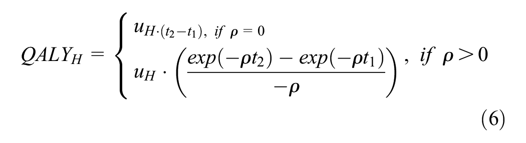
QAL Y_{H} = {\begin{matrix} u_{H \cdot (t_{2} - t_{1}), if ρ = 0} \\ u_{H} \cdot (\frac{\exp (- ρ t_{2}) - \exp (- ρ t_{1})}{- ρ}) \end{matrix}, if ρ > 0

(6)

where u_H is the utility weight of time spent in the “Home” state; ρ is the continuous, annual discount rate = ln(1 + r); t₁ is the years elapsed on entry into the “Home” state; and t₂ = t₁ + t_abs.

To compare the average computation times, the average numbers of cycles to compete absorption, and average, discounted, incremental QALE output of the 3 hospital discharge model structures (FCL, DCL, and DCL-pDES), we ran 5,000 replicates of each model version with 1,000 individuals per replicate. We estimated the model run time from the difference between the computer clock time at the beginning and end of a replicate. We calculated summary statistics and kernel density plots of the runtimes, numbers of cycles to completion, and incremental QALE across the 5,000 replicates.

An Open, Parallel, Surgical Wait-Time Model

We built a single-strategy, open, parallel microsimulation cost-utility model with a pDES component to emulate a surgical wait-list (Supplemental Figure 2).⁶ We modeled 10 operating room (OR) slots being available per weekly cycle. Individuals referred for surgery were placed on a wait-list where they were prioritized according to 4 levels of severity. We built 3 versions of the model: for the fixed exit horizon, the simulation ceased at 52 wk; for the fixed entry horizon, individuals who entered the model prior to 52 wk were observed until absorption, but no new individuals could enter the model after 52 wk; and for the fixed entry horizon plus phantoms version, new evaluated individuals could enter the model until 52 wk and then be observed until absorption. After 52 wk, phantoms entered the model at the same rate as evaluated individuals entered prior to the horizon. On each cycle, the number of new evaluated individuals or phantoms entering the wait-list was drawn from a Poisson distribution with a mean of 12. After entry, individuals were assigned surgical priorities and competed for operating room resources with other individuals, either phantoms or evaluated.

While on the wait-list, individuals could proceed to surgery, develop more severe disease and shift to a higher priority, or remain stable at the same priority level. At the end of each cycle, the wait-list was sorted by priority and then by wait time. Available OR slots for the following week were then assigned to the evaluated or phantom individuals at the top of the wait-list. Evaluated individuals who obtained surgery and survived were removed from the wait-list and entered the “postsurgery” pDES component, where they made a single transition to absorption in a similar fashion to absorption from the “Home” state in the hospital discharge model. Phantoms who received surgery were simply removed from the wait-list. Evaluated individuals accrued QALYs and costs as they transitioned from the wait-list until death while phantoms did not. We plotted the number of individuals on the wait-list per week of simulation for a single replicate of each version of the model and then ran 5,000 replicates each with 1,000 individuals of each model type in order to provide summary statistics and kernel density plots of the distributions of costs and QALE.

The FCL, DCL, and DCL-pDES models and the 3 versions of the surgical wait-list model were built in TreeAge 2022 R2.¹⁰ Supplemental Tables 1 and 2 provide model input variables and root expressions. For the surgical wait-list models, we made use of the Python coding utility in TreeAge to execute these operations with code provided in the supplemental appendix. Models were run on a virtual computer with 70 cores and 120,000 Mb of random access memory and are available at https://github.com/dnaimark/DCLpaper. Kernel density plots were generated in R v4.4.1.

Results

Comparisons of FCL, DCL, and DCL-pDES Hospital Discharge Models

The FCL structure took the longest to run, averaging 515 s per replicate (95% credible interval [CI]: 477 to 545) and required an average of 8,630 cycles to completion (95% CI: 8,340 to 8,920; Figure 2). The DCL method was faster, averaging 2.70 s (95% CI: 1.48 to 2.92) and required an average of 36.7 cycles to completion (95% CI: 35.7 to 37.6). The hybrid DCL-pDES structure was fastest, averaging 1.45 s (95% CI: 1.26 to 2.61) and required an average of 14.5 cycles to completion (95% CI: 14.1 to 14.9). Kernel density plots of incremental, discounted QALE denominated in QALYs (i.e., QALE_strat2– QALE_strat1) are shown in Figure 3. The means and distributions of incremental QALE across the 5,000 model replicates were similar among the 3 model structures. Kernel density plots for the outputs for each strategy for each model structure are shown in Supplemental Figure 1.

Figure 2

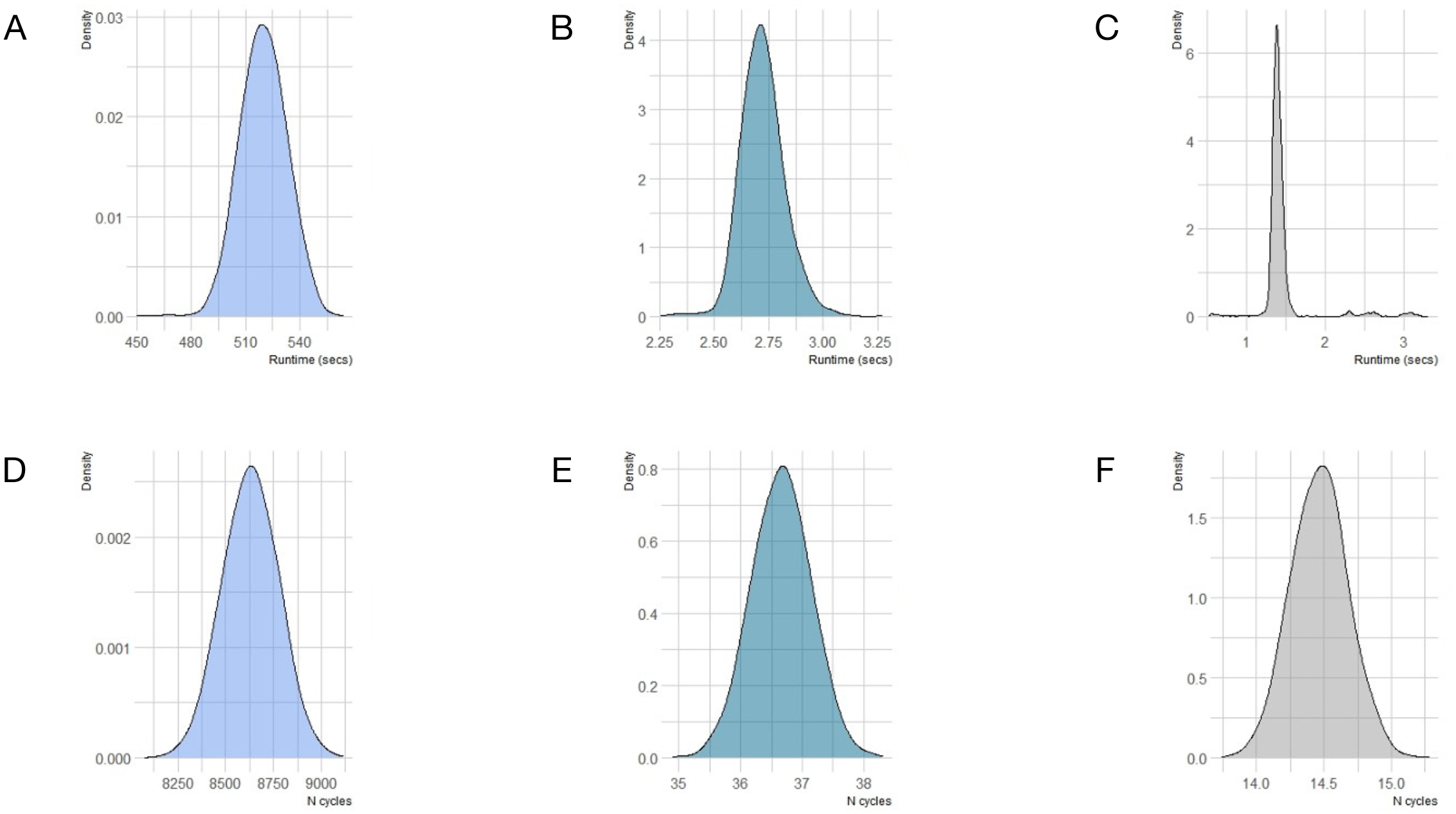
Kernel density plots of runtimes in seconds (A, B, and C) and numbers of cycles until complete absorption (D, E, and F) across 5,000 replicates for the 3 model structures, fixed cycle length (FCL), dynamic cycle length (DCL), and the hybrid model structure (DCL plus pseudo-discrete event simulation elements; DCL-pDES), respectively.

Figure 3

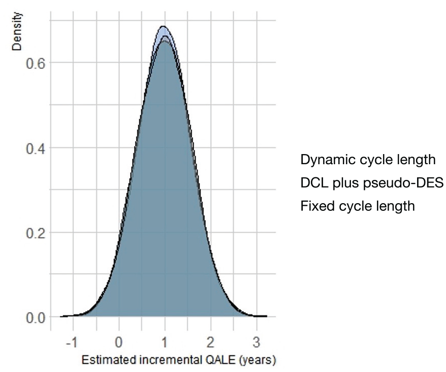
Kernel density plot of quality-adjusted life expectancy (QALE) outputs across 5,000 replicates of the 3 model strictures, fixed cycle length (fcl), dynamic cycle length (dclfullyr) and the hybrid model structure (DCL plus pseudo-discrete event simulation elements; dclpdes).

Comparisons of the Fixed Exit, Fixed Entry, and Fixed Entry with Phantoms Open, Parallel, Surgical Wait-List Models

For a single replicate of n = 1,000 individuals, the fixed exit version truncated trajectories of individuals, and the fixed entry version resulted in a more rapid decline in wait-list occupancy relative to the version with a fixed entry horizon and phantoms (Figure 4). Average lifetime, discounted costs, and QALE for the fixed exit version were $20,055 (95% CI: $19,000 to $21,120) and 14.2 QALYs (95% CI: 13.2 to 15.2), respectively; for the fixed entry version, the outputs were $27,030 (95% CI: $24,680 to $29,412) and 20.5 QALYs (95% CI: 20.0 to 20.9), respectively. These versions underestimated costs and QALE relative to the fixed entry with phantoms version, whose average outputs were $33,424 (95% CI: $27,510 to $44,484) and 20.5 QALYs (95% CI: 20.1 to 21.0), respectively. Kernel density plots of discounted, discounted costs, and QALE for the 3 versions are shown in Figure 5.

Figure 4

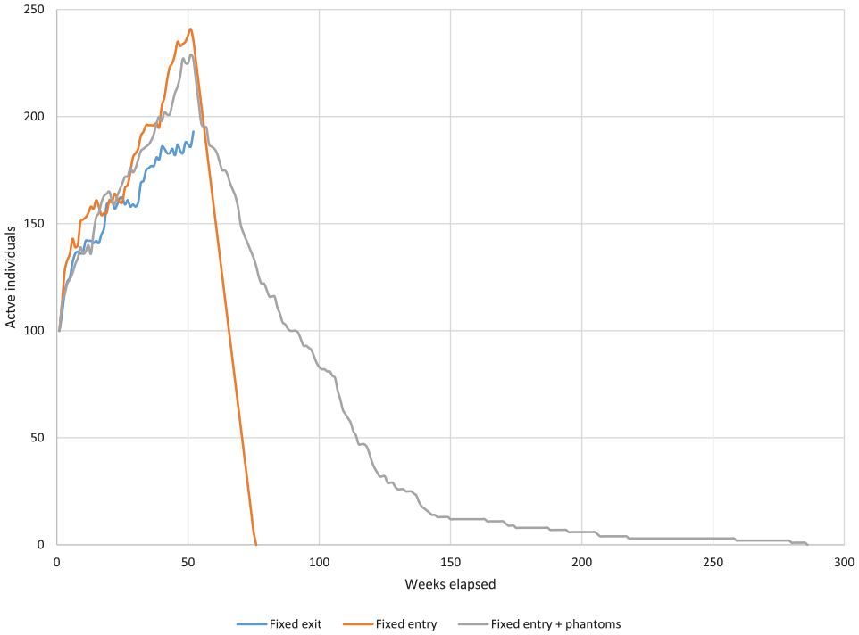
A graph for a single replicate of the surgical wait-list example model with numbers of active (“evaluated”) individuals as a function of model runtime in weeks for the fixed exit (blue), fixed entry (orange), and fixed entry plus phantoms structures (gray).

Figure 5

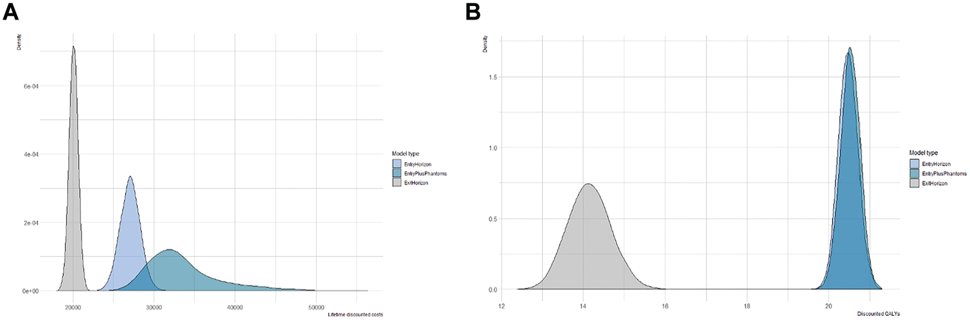
Kernel density plots of lifetime discounted costs (A) and discounted, quality-adjusted life expectancy (QALE; B) across 5,000 replicates of the 3 surgical wait-list model structures: fixed exit (gray), fixed entry (light blue), and fixed entry plus phantoms (teal).

Discussion

In this article, we describe how DCLs in microsimulation models reduce computational burden compared with FCLs and yield comparable incremental QALE output values for a 2-strategy, 4-state, hospital-discharge model. A further improvement in computation time was achieved by creating a hybrid model that incorporated a pseudo-DES feature into the DCL structure. We acknowledge that employing vector and matrix manipulations in simulation models (vectorization) may be more efficient than the methods we propose. The latter may be of use where vectorization is either not possible or overly cumbersome. We note that the relative performance of these modeling approaches will be context dependent: efficiency gains of DCL and DCL-pDES compared with FCL models will depend on the cycle length of the short-term states relative to the length of time to the model horizon.

The incremental QALE distributions were almost identical for the 3 hospital discharge model versions, and yet the QALE values for each strategy differed slightly among structure types, as shown in the supplement. This was a consequence of the fact that changes in time management affected QALE estimates to the same degree for the 2 strategies such that incremental QALE was the same across model versions. In practice, we expect that there may be differences among incremental costs and QALYs generated by each type of model structure.

The DCL structure has a limitation. Because of the loss of the direct connection between elapsed time and multiples of the cycle counter, DCL methods cannot easily be used in Markov cohort models unless the model structure does not allow backflows. In the latter case, the quasi-absorbing state could be modeled as the mean of a time-to-event distribution. In the case of the Gompertz distribution, there are methods to numerically estimate the mean.¹¹ In individual-level models, however, because cycle length is defined locally for each state, back transitions from chronic back to acute disease phases would not be problematic.

The FCL, DCL, and DCL-pDES model structures potentially require scaling the length of time over which per-cycle probabilities operate. For this article, we assumed direct observation of pairwise state transitions to which parametric Weibull survival models were fit in the short-term portion of the model. In more realistic situations, analysts may have access only to panel data consisting of a matrix of counts or transition probabilities observed after a duration of time longer than a state’s cycle length. In these cases, conversion of the latter probabilities to rates, scaling down to a shorter time frame, and then converting back to probabilities may lead to biased transition probability estimates over a cycle. Two potential solutions to this issue include eigenvector decomposition¹² and the use of the matrix exponential.¹³ However, if data on the rate of change of state membership exist in terms of a system of linear, first-degree, ordinary differential equations, eigenvector decomposition and the matrix exponential can be combined to yield the scalable transition probability estimates required by the DCL microsimulation structure as we show in the supplement. Such systems may be derived from multistate survival models estimated from real-world, observed individual-level data or constructed from literature estimates of pairwise, instantaneous rates of transition.

For convenience, we sampled the time from entry into the “Home” state to absorption in the hybrid DCL-pDES model from the Ontario general population using a parametric Gompertz distribution that was fit to life tables.⁸ The best-fitting distribution parameters by age were found by Resende et al.⁸ using a process of simulated annealing. R code is presented in the appendix of that article, which can be used to determine optimum Gompertz parameters by age for other jurisdictions given population life-table data. For low- and middle-income countries, with exaggerated infant and older adult death rates, general population mortality may not be well-represented by parametric Gompertz models. In these cases, nonparametric cumulative density functions based on local mortality tables could be sampled for times to death. For some diseases, the risk of death may be dominated by disease-specific causes rather than general population mortality rates, yet long-term survival data may not be available. This may require parametric extrapolation of survival curves and then sampling from the resulting time-to-death distribution.

The use of a hybrid model, apart from being more computationally efficient, is also an efficient way to model long-term events for individuals who survive an initial, open, parallel model structure for the purposes of economic evaluation. However, the hybrid structure creates a conflict between the model’s time horizon and the horizons of the individuals who traverse it. We describe how the use of phantoms can overcome this horizon problem. For illustration, we set time spent on the wait-list to be quite costly relative to time spent after the operation in the surgical wait-list example model. In practice, we expect that the difference in lifetime costs and QALE between the fixed entry and fixed entry with phantom structures will depend on the magnitude of these quantities generated while on the wait-list.

Conclusion

Changing from fixed to DCLs may reduce computation time for microsimulation models. Incorporation of discrete-event-simulation-like components may provide further efficiency. The latter may also be used to efficiently model long-term costs and QALE in an open, parallel model context provided the inherent horizon problem is addressed through the use of phantoms.

Supplemental Material

sj-docx-1-mdm-10.1177_0272989X251319808 – Supplemental material for Changing Time Representation in Microsimulation Models

Supplemental material, sj-docx-1-mdm-10.1177_0272989X251319808 for Changing Time Representation in Microsimulation Models by Eric Kai-Chung Wong, Wanrudee Isaranuwatchai, Joanna E. M. Sale, Andrea C. Tricco, Sharon E. Straus and David M. J. Naimark in Medical Decision Making

Footnotes

The authors declared no potential conflicts of interest with respect to the research, authorship, and/or publication of this article. The authors disclosed receipt of the following financial support for the research, authorship, and/or publication of this article: This study was not funded. Eric Kai-Chung Wong is supported by a Vanier Scholarship (Canadian Institutes of Health Research) and the Clinician Scientist Training Program at the University of Toronto. Sharon E. Straus is supported by a Tier 1 Canada Research Chair. Andrea C. Tricco is supported by a Tier 1 Canada Research Chair in Knowledge Synthesis.

ORCID iDs

Eric Kai-Chung Wong

Joanna E. M. Sale

Andrea C. Tricco

David M. J. Naimark

Research Data

No data were required for this article. Models used in the article are available at .

References

Caro

Briggs

Siebert

, et al. Modeling good research practices–overview: a report of the ISPOR-SMDM Modeling Good Research Practices Task Force—1. Value Health. 2012;15:796–803.

Siebert

Alagoz

Bayoumi

, et al. State-transition modeling: a report of the ISPOR-SMDM Modeling Good Research Practices Task Force-3. Med Decis Making. 2012;32:690–700.

Karnon

Stahl

Brennan

, et al. Modeling using discrete event simulation: a report of the ISPOR-SMDM Modeling Good Research Practices Task Force-4. Med Decis Making. 2012;32:701–11.

Naimark

DMJ

Kabboul

Krahn

. The half-cycle correction revisited: redemption of a kludge. Med Decis Making. 2013;33:961–70.

Elbasha

Chhatwal

. Theoretical foundations and practical applications of within-cycle correction methods. Med Decis Making. 2016;36:115–31.

Naimark

. dnaimark/DCLpaper. 2023. Available from: https://github.com/dnaimark/DCLpaper. [Accessed 2 November, 2023].

El-Gohary

Alshamrani

Al-Otaibi

. The generalized Gompertz distribution. Appl Math Modell. 2013;37:13–24.

Resende

MHF

Yarnell

D’Souza

, et al. Clinical decision analysis of elective delivery vs expectant management for pregnant individuals with COVID-19–related acute respiratory distress syndrome. Am J Obstet Gynecology MFM. 2022;4(6):100697 DOI: 10.1016/j.ajogmf.2022.100697.

Lee

McCarron

. Guidelines for the Economic Evaluation of Health Technologies: Canada—4th Edition. Ottawa (Canada): CADTH; 2017. Available from: https://www.cadth.ca/sites/default/files/pdf/guidelines_for_the_economic_evaluation_of_health_technologies_canada_4th_ed.pdf. [Accessed 2 November, 2023].

10.

TreeAge. Treeage Pro 2022 R.2. 2022. Available from: http://www.treeage.com.

11.

Giao

. Revisit of well function approximation and an easy graphical curve matching technique for theis’ solution. Groundwater. 2003;41:387–90.

12.

Chhatwal

Jayasuriya

Elbasha

. Changing cycle lengths in state-transition models: challenges and solutions. Med Decis Making. 2016;36:952–64.

13.

Moler

Van Loan

. Nineteen dubious ways to compute the exponential of a matrix, twenty-five years later. SIAM Review. 2003;45:3–49.

Supplementary Material

Please find the following supplemental material available below.

For Open Access articles published under a Creative Commons License, all supplemental material carries the same license as the article it is associated with.

For non-Open Access articles published, all supplemental material carries a non-exclusive license, and permission requests for re-use of supplemental material or any part of supplemental material shall be sent directly to the copyright owner as specified in the copyright notice associated with the article.

0.00 MB

0.26 MB