Sage Journals: Discover world-class research

Abstract

This tutorial aims to help make the best available methods for generating and presenting cost-effectiveness results with uncertainty common practice. We believe there is a need for such type of tutorial because some erroneous practices persist (e.g., identifying the cost-effective intervention as the one with the highest probability to be cost-effective), while some of the more advanced methods are hardly used (e.g., the net loss statistic ‘NL’, expected net loss curves and frontier). The tutorial explains with simple examples the pros and cons of using ICER, incremental net benefit and NL to identify the cost-effective intervention, both with and without uncertainty accounted for probabilistically. A flowchart provides practical guidance on when and how to use ICER, incremental net benefit or NL. Different ways to express and present uncertainty in the results are described, including confidence and credible intervals, the probability that a strategy is cost-effective (as usually shown with cost-effectiveness acceptability curves (CEACs)) and the expected value of perfect information (EVPI). The tutorial clarifies and illustrates why EVPI is the only measure accounting fully for decision uncertainty, and why NL curves and the NL frontier may be preferred over CEACs and other plots for presenting cost-effectiveness results in the context of uncertainty. The easy calculations and a worked-out real-life example will help users to thoroughly understand and correctly interpret key cost-effectiveness results. Examples with mathematical calculations, interpretation, plots and R code are provided.

Keywords

cost-effective plane cost-effective frontier net loss probabilistic sensitivity analysis cost-effective threshold willingness-to-pay threshold

Introduction

The cost-effectiveness of a health care intervention is an important criterion for policy. Different approaches exist to identify “the cost-effective” (“optimal”, “preferred”, “most attractive”, or “most cost-effective”) intervention among a set of alternatives. These approaches may use the concepts of (extended or “weak”) dominance and incremental cost-effectiveness ratios (ICERs) or net benefits. However, these are sometimes used inappropriately. For instance, in the context of uncertainty, the cost-effective intervention should be identified based on expected cost-effectiveness,¹ as this statistic accounts for both the probability that the intervention is not cost-effective (i.e., the probability to make a wrong decision) and the consequences of making a wrong decision.² Nevertheless, the cost-effective intervention is sometimes defined as the intervention with the highest probability to be cost-effective (e.g., as erroneously described in the guidelines of the Joint Committee on Vaccination and Immunisation).³ Furthermore, country-specific guidelines often lack detail. For instance, the Belgian guidelines on economic evaluation recommend to present uncertainty around the ICER with a confidence or credible interval.⁴ However, it does not specify that this is only appropriate when all sampled values from the probabilistic sensitivity analysis result in positive incremental costs and health effects.⁵ Also, confidence and credible intervals do not necessarily inform about the extent of decision uncertainty.⁶

The expected net loss (NL) curves and frontier have been proposed in 2008^7,8 as a way to present in a single plot 1) the cost-effective intervention, 2) the expected value of information (i.e., the cost of uncertainty), and 3) how much better the cost-effective intervention is compared to its alternatives. However, despite its unique summarizing ability, this type of plot seems absent in many (country-specific) guidelines^9,10 and seems only exceptionally used by analysts.¹¹

With this tutorial, we aim to explain the best available methods for generating and presenting cost-effectiveness results under uncertainty, conceptually as well as through examples. Readers are expected to be familiar with some aspects of cost-effectiveness analysis (e.g., ICER), but this tutorial seeks to deepen and broaden their knowledge. For example, we explain the advantages and disadvantages of using ICER, incremental net benefit (INB), or NL as a measure for relative efficiency and why the information cost-effectiveness acceptability curves do not fully represent uncertainty around choosing the cost-effective strategy.

The tutorial starts from the cost and effect values obtained for each intervention option as part of an economic evaluation and accords to 4 principles.

First, the tutorial is constructed around key questions, rather than available methods: 1) How do you identify the cost-effective intervention from a set of alternatives? And 2) how do you measure and interpret (decision) uncertainty? Readers are directed toward the various methods to answer these questions (summarized in a flowchart), as well as appropriate ways to present their results. Pros and cons of each method are described and illustrated with simple examples. Practical guidance is provided on when (not) to use which method.

Second, the tutorial shows how to identify the cost-effective strategy with ICER, INB, and NL both without and with uncertainty accounted for in a probabilistic way. Although the NL statistic has been introduced for its attractive properties when dealing with uncertainty,⁸ we believe it is easier to grasp the link between ICER, INB, and NL without the additional complexity of uncertainty.

Third, the tutorial distinguishes 1) the information that needs to be obtained to answer each key question (usually in the form of estimated values) and 2) the different ways this information can be presented (e.g., using a table or a plot). This explicit distinction between plots and their underlying information should help readers to thoroughly understand which key cost-effectiveness results are appropriate to answer their questions and choose correct display methods for these results.

Fourth, the examples and associated calculations (e.g., to calculate ICER, INB, NL, and expected value of perfect information [EVPI]) are kept simple to allow deeper understanding of the basic concepts and assume no knowledge of particular software. However, a more complex worked-out real-life example is included that further illustrates how the use of inappropriate methods or the incorrect use of appropriate methods can result in wrong conclusions.

Basic Concepts

A health economic evaluation compares different interventions in terms of both their costs and benefits.¹² Usually, determining the cost-effective intervention will involve calculating a measure for cost-effectiveness and comparing this to a cost-effectiveness (“willingness-to-pay”) threshold k. In this tutorial, we are assuming that basic conceptual choices, such as the consideration of all viable intervention options and the determination of a (range of) k values, are made appropriately.^12,13

Measures for Cost-Effectiveness

Depending on the study question and comparison undertaken, different outcome measures may be of interest, such as the average cost-effectiveness ratio and the marginal cost-effectiveness ratio, but we focus on the most commonly used: the incremental cost-effectiveness ratio and the incremental net benefit.¹²

An incremental cost-effectiveness ratio (ICER) compares the difference between the costs (“C”) and health outcomes (effects “E”) of 2 mutually exclusive interventions that compete for the same resources and is generally described as the additional cost per additional health outcome:

ICER = \frac{C_{intervention A} - C_{intervention B}}{E_{intervention A} - E_{intervention B}}

The ICER numerator includes the difference in program costs and can include in addition the averted disease costs and averted productivity losses depending on the choice of perspective.

The INB puts the differences in costs and health outcomes on the same scale by using a threshold k, that is, the value one is willing to pay for a 1-unit health effect (e.g., a quality-adjusted life year). The incremental net monetary benefit (INMB) rescales differences in effects (“incremental effects”) in monetary terms by multiplying it with the cost-effectiveness threshold and then subtracting the cost difference (“incremental costs”):

INMB = [(E_{intervention A} - E_{intervention B}) * k] - (C_{intervention A} - C_{intervention B})

The incremental net health benefit (INHB) rescales incremental costs in health effect terms by dividing it by k and subtracting it from the incremental effects:

INHB = (E_{intervention A} - E_{intervention B}) - [\frac{(C_{intervention A} - C_{intervention B})}{k}]

Note that when using INMB or INHB, a k value needs to be assumed explicitly. However, also when using the ICER for policy making, in most cases, a threshold needs to be considered in order to decide if an intervention is cost-effective or not (see next section).

The cost-effectiveness threshold and decision making

Health care interventions can be considered relatively cost-effective if their ICER lies below k or—equivalently—if the intervention results in a net benefit (and not a loss, i.e., a positive INB) (Table 1).¹⁴ When an intervention results in money savings but is less effective (health loss), it is cost-effective when its ICER is higher than k (Table 1).¹⁴ Consistent use of k can improve decision making, as it sets a standard that allows optimizing the total sum of achievable health gains under a budget restriction.

Table 1

Decision Rules for Cost-Effectiveness of Intervention B Compared to Intervention A^a

Characteristic	B Cost-Effective Compared to A	B Not Cost-Effective Compared to A
ICER, when B costlier but more effective than A	<k	≥k
ICER, when B less costly but less effective than A	>k	≤k
INMB or INHB for k	>0	<0

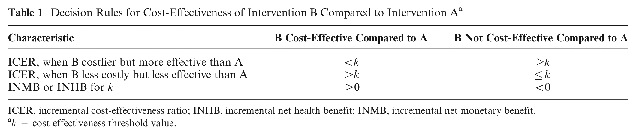
ICER, incremental cost-effectiveness ratio; INHB, incremental net health benefit; INMB, incremental net monetary benefit.

k = cost-effectiveness threshold value.

Methods on how to determine a value for k are still being debated.¹⁵ There is no “one-size-fits-all”k for all countries. Each country is encouraged to establish their own k, reflecting local preferences.¹⁶ The choice of k is related to budget restrictions and local value judgments on efficiency-equity tradeoffs and may be guided by the ICERs of previous interventions to stimulate consistent policymaking.

Answering Key Cost-Effective Questions

We consider 2 distinct questions: (1) How do we identify the cost-effective intervention from a set of alternatives? (2) How do we measure and interpret decision uncertainty?

The first section answers the first question, depending on whether 2 or more interventions are compared and whether uncertainty was accounted for in a probabilistic way. Uncertainty is accounted for in a probabilistic way if the uncertainty around model choices and input parameters is defined as probability distributions, from which then typically n random samples are drawn to calculate the corresponding n cost and n health effect values for each intervention considered (a process referred to as probabilistic sensitivity analysis [PSA]). In particular, we show the equivalence of using ICER, INMB, or INHB to identify the cost-effective intervention, in both the absence and the presence of uncertainty, and we introduce the NL statistic.

The second section describes how the key measure that quantifies decision uncertainty (i.e., the expected value of information) can be obtained, the need to use the INB or NL approach to calculate it, and why it is superior to other popular measures of uncertainty (e.g., confidence and credible intervals).

The third section indicates how to best present cost-effectiveness results and decision uncertainty depending on the measure for cost-effectiveness used and the number of interventions compared.

The first 3 sections are illustrated in the fourth section with a worked-out real-life example and summarized in the fifth section.

Note that when some uncertainties are reflected as choices (scenarios) rather than probability distributions, the cost-effective intervention and associated decision uncertainty need to be obtained for each scenario separately.

Additional examples including mathematical calculations, plots, interpretation, and R code are provided in the Appendix.

How to Identify the Cost-Effective Intervention?

This is summarized in Figure 1, starting from the costs and effects obtained for each intervention under evaluation as part of an economic evaluation. When uncertainty is accounted for in a probabilistic way, this results in n cost and n effect values for each intervention, with n referring to the number of random samples drawn with PSA.

Figure 1

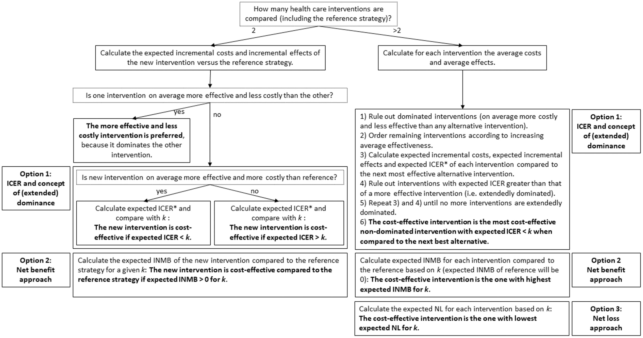
Flowchart to identify the cost-effective health care intervention, under conditions with and without uncertainty. The flowchart applies to the n cost and n effect values obtained in the economic evaluation for each intervention considered (including intervention costs and averted disease costs, depending on the perspective), with n reflecting the number of random samples drawn with probabilistic sensitivity analysis. Reference strategy refers to the intervention used as comparator, often “usual practice.”*Expected ICER of 1 strategy compared to its next best alternative needs to be calculated as the average incremental cost divided by the average incremental effect. All other expected values are calculated as averages across all n values for each strategy. When probabilistic uncertainty is not considered, the flowchart applies to the single cost and effect value obtained for each intervention considered (no averages need to be calculated). ICER, incremental cost-effectiveness ratio; INMB, incremental net monetary benefit; k, cost-effectiveness threshold; NL, net loss.

What is the cost-effective option from 2 interventions when no uncertainty is accounted for?

When the choice is between a new intervention and the reference strategy, there are 4 possible outcomes¹²:

- The new intervention dominates, that is, is both more effective and less costly than the reference strategy (Table 2, example 1).

- The new intervention is dominated, that is, is both less effective and more costly than the reference strategy (Table 2, example 2).

Table 2

Four Different Examples of Incremental Costs and Effects Outcomes of a New Intervention Compared to the Reference Strategy (“Usual Practice,” Not Explicitly Shown) and the Corresponding ICER, INMB, and INHB, Assuming an Arbitrary Willingness-to-Pay Value of €30,000 per Unit Health Gain

Example	Incremental Costs	Incremental Effects	ICER	INMB	INHB
1	−€200,000	10
2	€200,000	−10
3	€200,000	10	€20,000	€100,000	3
4	−€200,000	−10	€20,000	−€100,000	−3

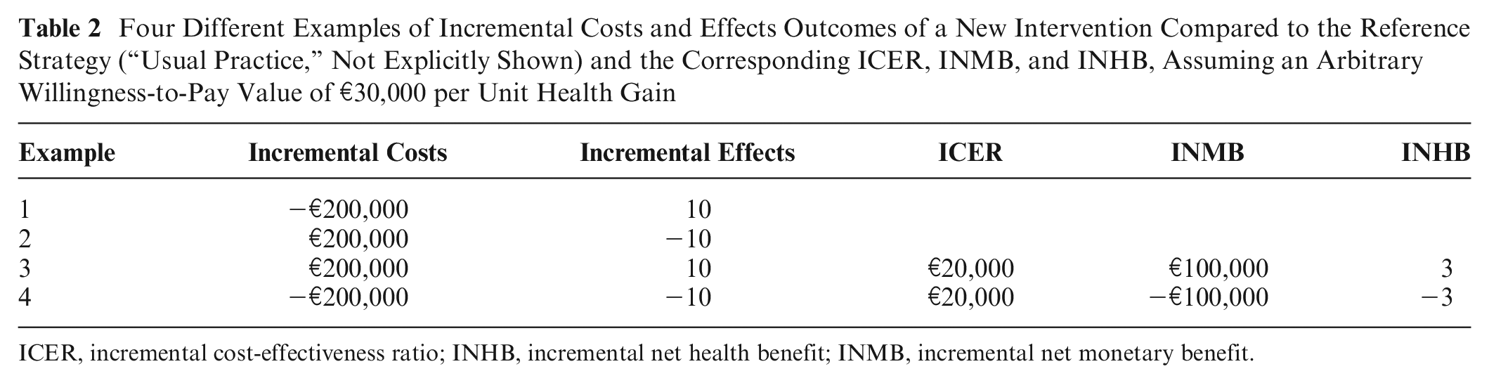
ICER, incremental cost-effectiveness ratio; INHB, incremental net health benefit; INMB, incremental net monetary benefit.

Note that if either (but not both) incremental costs or effects are negative, the ICER value is negative, and its magnitude therefore provides little information about the relative attractiveness of an intervention. Larger savings and more health gains are preferred but would have an opposite effect on the negative ICER, with larger savings driving the ICER toward negative infinity and larger health gains driving it toward zero.¹⁷

- The new intervention is both more effective and costlier than the reference strategy (Table 2, example 3). A cost-effectiveness measure needs to be calculated using the decision rules from Table 1. In Table 2 (example 3), the new intervention is cost-effective compared with the reference strategy at k of €30,000 per unit health gain, because the ICER of €20,000 per unit health gain is lower than k or, equivalently, because the INMB and INHB of the new intervention compared to the reference are positive.

- The new intervention is both less effective and less costly than the reference strategy. For example 4 in Table 2, the new intervention is cost-ineffective at a k of €30,000 per unit health gain, because the ICER of €20,000 per unit health gain is lower than k or, equivalently, because INMB and INHB are negative.

Although examples 3 and 4 (Table 2) result in the same ICER value, the interpretation is different despite the use of the same k: the new intervention is cost-effective in example 3 but cost-ineffective in example 4. Hence, the signs of the incremental costs and effects should always be reported separately with the ICER. With the INB approach, such problems of interpretation do not occur.⁵

What is the cost-effective option from more than 2 interventions when no uncertainty is accounted for?

In studies that compare more than 2 mutually exclusive interventions, historically, the concepts of strong dominance and extended dominance (sometimes called “weak dominance”) were applied, using the ICER as a measure for cost-effectiveness.^12,18,19 See Figure 1 for the general approach and Appendix 3.1.2 for examples including calculations, interpretation, and R code.

Alternatively, INB can be used. In the absence of an agreed-upon fixed k, INB values will have to be calculated for a range of k values. Importantly, the distance between k values considered needs to be small enough to detect interventions that are cost-effective for only a small range of plausible k values. The ICER does not suffer from this problem as it is calculated independently of k. However, using INB, no pairwise comparisons are necessary, as the INB between any 2 interventions is simply the difference between the INB of the 2 interventions compared to the same common reference strategy.⁵ Hence, when using INB as measure for cost-effectiveness, it is sufficient to calculate for each intervention 1 INB value, whereas when using the ICER, additional ICER values may need to be calculated (e.g., Appendix example 3.1.2.1).

Although the ordering across interventions based on INB does not depend on the chosen reference strategy (comparator), the absolute value of INB does depend on the chosen reference strategy when comparing more than 2 interventions. For instance, if we would have chosen intervention A as reference for the example in Appendix example 2.1.2.1, INMB of intervention C v. A would be €20,000 as opposed to €45,000 with reference “do nothing” (Table 3). Therefore, the INB of the cost-effective intervention does not directly reflect how much better this intervention is compared to the alternatives.

Table 3

Example of Incremental Net Monetary Benefit (INMB) and Net Loss (NL) When Comparing More Than 2 Interventions, without Considering Probabilistic Uncertainty^a

Intervention	INMB v. Do Nothing	INMB v. A	NL v. Cost-Effective Intervention C
Do nothing	€0	−€25,000	€45,000 = €45,000 – €0 = €20,000 – (–€25,000)
A	€25,000	€0	€20,000 = €45,000 – €25,000 = €20,000 – €0
B	€40,000	€15,000	€5000 = €45,000 – €40,000 = €20,000 – €15,000
C	€45,000	€20,000	€0 = €45,000 – €45,000 = €20,000 – €20,000

INMB is calculated based on Appendix example 3.1.2.1 using either “do nothing” or intervention A as reference strategy and assuming an arbitrary cost-effectiveness threshold of €20,000 per quality-adjusted life year gained.

The NL statistic (“opportunity cost”) overcomes this problem, because it does not depend on the choice of the reference intervention.⁸ The NL of an intervention is calculated as the difference in INMB of that intervention with the INMB of the cost-effective intervention (= intervention with highest INMB), for a given k:

$N L_{h} = INM B_{\max} - INM B_{h}$ , for intervention h from a set of interventions (h = 1, . . ., H)

Indeed, the NL for each intervention in our example is the same when using “do nothing” or intervention A as the reference strategy (Table 3). When not considering uncertainty with PSA, the NL of the intervention resulting in highest INMB for a given k is €0. The NL statistic has been introduced as an alternative to INB for evaluations accounting for uncertainty in a probabilistic way (see next section).^8,20

What is the cost-effective intervention when uncertainty is accounted for in a probabilistic way?

When uncertainty is accounted for in a probabilistic way, this results in n cost and n effect values for each intervention, with n referring to the number of random samples drawn with PSA. The same methods as when no uncertainty is accounted for can be used to identify the cost-effective intervention in the context of uncertainty but need to be applied to the expected measure of cost-effectiveness (Figure 1).¹ For worked-out examples including R code, see Appendixes 3.2 and 3.3.

The (extended) dominance principle can be applied on the average and incremental cost and effect values, followed by calculating pairwise expected ICER values. Note that the expected ICER of an intervention compared to an alternative intervention needs to be calculated as the average incremental costs divided by the average incremental effects.¹⁷

Alternatively, the expected INMB or INHB for each intervention can be calculated when compared to the reference strategy, as the average across all n INMB or INHB values.

The expected NL for each intervention can be calculated as the average across all n NL values. The NL for 1 sample of an intervention is the NL of that intervention when compared to the cost-effective intervention (i.e., intervention with highest INMB) for that sample. The cost-effective intervention is the intervention with the lowest expected NL. As such, unlike INMB or INHB, the NL and expected NL statistics by design always compare to the appropriate lowest NL comparator. Note that the expected NL value calculated here also represents the extent of decision uncertainty (see next section).^8,20

In the absence of an agreed-upon k, the n INMB, INHB, or NL values and the expected INMB, INHB, or NL values for each intervention considered need to be calculated over a range of k values.

Although all 4 cost-effectiveness summary measures (ICER, INMB, or INHB and NL) are equivalent for identifying the cost-effective intervention, they cannot all be used to estimate the extent of decision uncertainty (see next section). Only the NL statistic can be used to identify directly the cost-effective intervention, the extent of decision uncertainty, and how much better the cost-effective intervention is compared to alternatives.

How to Measure and Interpret the Extent of Decision Uncertainty Surrounding the Cost-Effective Results?

Decisions need to be made in the context of uncertainty. The cost-effective intervention is the intervention that is on average cost-effective, irrespective of the degree of uncertainty. This means that the use of confidence and credible intervals as a measure for decision uncertainty should be avoided because they should not have an impact on our intervention of choice given current evidence.^5,6 Still, it is important to account for uncertainty in a correct (i.e., probabilistic) way for 2 reasons: 1) to estimate expected ICER, INMB, and/or NL values correctly in case of nonlinear relationships between input parameters and model outcomes and 2) to provide decision makers with additional information: the expected opportunity loss (“NL”) of deciding under uncertainty today. Indeed, uncertainty gives rise to a probability of making a wrong decision and the consequences of making that wrong decision (i.e., the NL).

The probability of making a wrong decision equals 1 minus the probability that the intervention identified as cost-effective (i.e., based on expected ICER, INMB, and/or NL) is cost-effective. It is calculated as the proportion of the n samples that an intervention is cost-effective compared to the alternatives, either based on the ICER or the INMB.²¹ In Table 4, B is the cost-effective intervention (highest expected INMB) but only has a 25% probability to be cost-effective (highest INMB in only 1 of 4 samples). In other words, the probability of making a wrong decision (i.e., that choosing intervention B would be wrong) in this example is 75%. Often these probabilities are plotted as cost-effectiveness acceptability curves (CEACs; Appendix 1.4).^5,22

Table 4

Incremental Net Monetary Benefit (INMB) and Net Loss (NL) of 3 Strategies (Existing Strategy E, New Strategy A, and New Strategy B)^a

Sample	INMB: E v. E	INMB: A v. E	INMB: B v. E	NL E	NL A	NL B
1	€0	−€38,400	−€38,500	€0	€38,400	€38,500
2	€0	€1,950	€1,900	€1,950	€0	€50
3	€0	€2,300	€36,200	€36,200	€33,900	€0
4	€0	€28,200	€1,700	€28,200	€0	€26,500
Average	€0	−€1,488	€325	€16,588	€18,075	€16,263

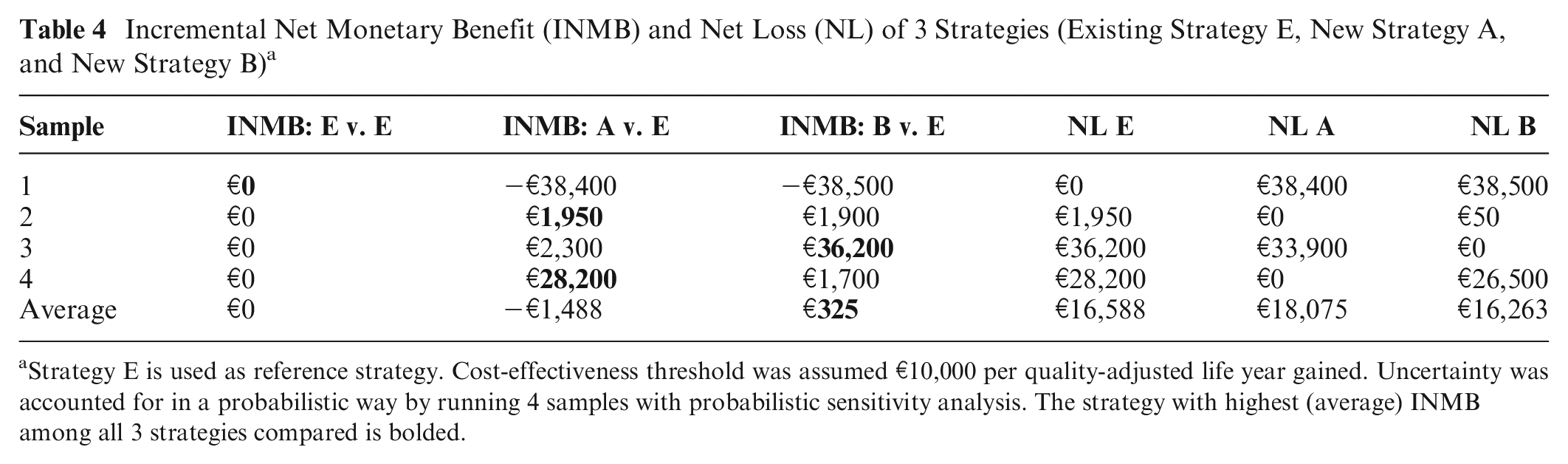
Strategy E is used as reference strategy. Cost-effectiveness threshold was assumed €10,000 per quality-adjusted life year gained. Uncertainty was accounted for in a probabilistic way by running 4 samples with probabilistic sensitivity analysis. The strategy with highest (average) INMB among all 3 strategies compared is bolded.

These probabilities inform us about 1) whether or not decision uncertainty exists (if the probability that an intervention is identified as cost-effective is 100%, no decision uncertainty exists), 2) the magnitude of decision uncertainty (a high probability to be identified as cost-effective indicates less decision uncertainty than a low probability), and 3) which other interventions have some probability of being cost-effective.¹² Importantly, these probabilities do not indicate whether this decision uncertainty “matters.”

The consequences of making a wrong decision refer to the NL when choosing a suboptimal intervention. For the example shown in Table 4, intervention B results in highest INMB only in sample 3. Net loss of choosing B over A and E is €38,500, €50, and €26,500 for samples 1, 2, and 4, respectively. Expected NL for B can be calculated as the average of the NL for B over all samples (Table 4). Equivalently, expected NL for B can be calculated as the product of the probability that B is suboptimal (in Table 5: 75%) times the average NL only for the samples where B is suboptimal: (€38,500 + €50 + €26,500)/3 = €21,683. Indeed, 0.75 * €21,683 = €16,263. Intervention A has 50% probability to be cost-effective. However, NL when not cost-effective is large: €38,400 for sample 1 and €33,900 for sample 3, resulting in an average NL for the samples where A is suboptimal of (€38,400 + €33,900)/2 = €36,150. Although A has a higher probability to be cost-effective than B (50% compared to 25%), NL of A when suboptimal is also higher than B (€36,150 compared to €21,683). This is why A would result in a higher expected NL than intervention B (€18,075 > €16,263; Table 4). A full picture of decision uncertainty requires both the probability of making a wrong decision and its consequences. Therefore, the expected NL of the cost-effective intervention given current information (“the cost of uncertainty”) (€16,263 for example in Table 4) is considered the current best measure for decision uncertainty and is also referred to as the EVPI.^6,23 It represents the price that one is willing to pay to have perfect information regarding all uncertain aspects of the disease and interventions under study that influence which intervention is preferred based on cost-effectiveness analysis. If EVPI given current information is larger than the cost of designing and conducting studies to obtain perfect information on all uncertain aspects of the disease and health care strategies under study, then further research may be justified (a necessary but not sufficient condition). In the example shown in Table 4, the cost-effective strategy B has an EVPI of €16,263. This amount indicates that studies that allow estimating model data and parameters more precisely and therefore choosing the cost-effective strategy with more certainty may only be justifiable if those studies jointly cost less than €16,263. Importantly, EVPI depends on k and is usually obtained and presented for a range of k values (see further real-life example). EVPI can be expressed per patient or for a specific population. To obtain the population EVPI, estimates of the population of patients that is expected to benefit from the additional information and the time horizon over which the evidence is expected to be useful are needed.

Table 5

Expected Incremental Costs, DALYs Averted, and ICER for 4 Typhoid Conjugate Vaccination Options in Nepal: No Vaccination (NOVAC), Routine Childhood Vaccination (R), R plus Onetime Catch-up Campaign up to Age 5 Years (RC5), and R plus Onetime Catch-up Campaign up to Age 15 Years (RC15)^a

Comparison	Expected Incremental Costs, USD	Expected DALYs Averted	Expected ICER Calculated as Expected Incremental Costs Divided by Expected DALYs Averted, USD
NOVAC v. NOVAC	0	0	NA
R v. NOVAC	16,974,084	62,264	272/DALY averted
RC5 v. NOVAC	20,442,645	91,736	223/DALY averted
RC15 v. NOVAC	29,346,750	123,859	237/DALY averted
RC15 v. RC5	8,904,105	32,124	277/DALY averted

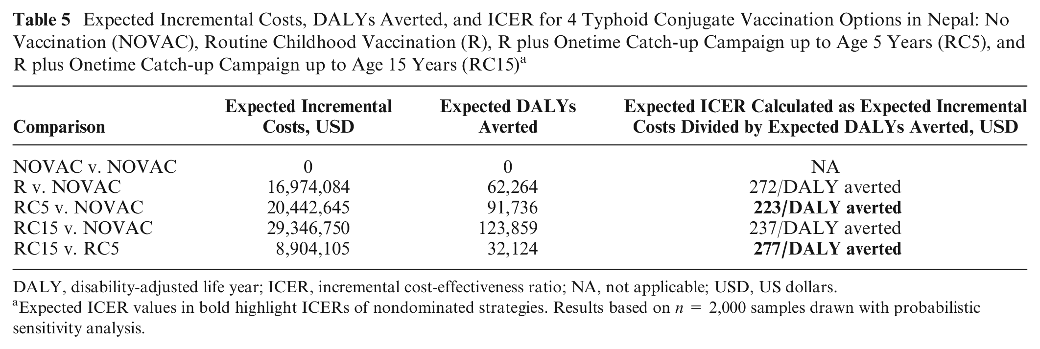
DALY, disability-adjusted life year; ICER, incremental cost-effectiveness ratio; NA, not applicable; USD, US dollars.

Expected ICER values in bold highlight ICERs of nondominated strategies. Results based on n = 2,000 samples drawn with probabilistic sensitivity analysis.

A difficulty with the EVPI is that it is not straightforward to interpret. In practice, it will rarely be possible to obtain perfect information about all uncertain aspects in a new study (i.e., to eliminate uncertainty completely). Therefore, it is useful to obtain an EVPI value for each uncertain parameter separately and/or for groups of uncertain parameters (referred to as EVPPI values).²⁴ EVPPI values can be used to rank the importance of the uncertain input parameters. The uncertain parameter with the highest EVPPI value has the most influence on which intervention is cost-effective and therefore has the highest value of obtaining more evidence. The uncertainty of parameters with EVPPI values equal to €0 has no impact on which intervention is cost-effective. The real-life example (see further) includes an example of EVPPIs and their interpretation.

However, the EVPI and EVPPI values do not answer the question, “Can further research be worthwhile?”²⁵ It may therefore be relevant to calculate the expected value of sample information (EVSI) and the expected net benefit of sampling (ENBS). EVSI can be calculated for each uncertain parameter separately and/or for groups of uncertain parameters. ENBS is the difference between EVSI and the cost of sampling. A disadvantage is, however, that the calculation of EVSI and ENBS requires additional information on the cost and expected benefits of conducting particular research, which may introduce additional uncertainties.¹² Therefore, we recommend always calculating EVPI and EVPPIs as they can be easily obtained based on the probabilistic sensitivity analysis sample of the economic evaluation. Importantly, EVPI and EVPPI indicate whether further research may be justifiable, but they cannot be used to decide whether additional research is required.

How to Report or Present Main Cost-Effectiveness Results?

When using ICER as measure for cost-effectiveness, a table can be informative to illustrate the different steps involved in applying the concepts of (extended) dominance (Appendix 1.1). It should include costs and effects per intervention and pairwise ICER values. When uncertainty is accounted for with PSA, the same table can be used but showing average costs, effects, and pairwise expected ICER values. When only 2 interventions are compared, it can be sufficient to just mention in text (average) incremental costs, (average) incremental effects, and (expected) ICER of the new intervention compared to the reference strategy. It is often insightful to also present these results on the incremental cost-effectiveness plane (Appendix 1.2).²⁶ Note that in the context of uncertainty, the average incremental cost and effect of each intervention compared to the reference strategy need to be shown on the plot, in addition to the n incremental cost and effect values, to assess which intervention is cost-effective given k. When comparing more than 2 interventions in the context of uncertainty, the cost-disutility plane may offer better insight in incremental costs and effects, because they are compared to the appropriate lowest cost and highest effect comparator for each sample (Appendix 1.6).

With the INB approach, simply describing the extent of the INB can be sufficient when the use of a single k applies, but if policy requires considering more than one k, it is preferable to show (expected) INB values for each intervention considered conditional on k in a table (Appendix 1.1) or on the INB plot (Appendix 1.3).²⁷

When using expected NL as a measure for cost-effectiveness, the cost-effective intervention for k can be easily identified from the expected NL plot (Appendix 1.7).^7,8,20 Alternatively, a table can report expected NL values for each intervention for a range of k values.

Importantly, the exact k value at which the cost-effective intervention changes (i.e., the crossing points on the plots) cannot easily derived from the expected INB and NL plots but can, for instance, be calculated as the expected ICER of the 2 interventions that are crossing (illustrated with the real-life example (see further) and in Appendix 1.3 [INMB plot] and 1.7 [NL plot]).

Note that the cost-effective intervention cannot necessarily be identified from CEACs (Appendix 1.4), except when the cost-effectiveness outcome follows a symmetrical distribution. This is because the intervention with highest probability to be cost-effective is not always the intervention that is on average most cost-effective (see example in Table 4).²⁸ For CEAC plots, preferably dotted rather than solid lines should be used. Solid lines may be interpreted as if probabilities have been obtained for “all”k values plotted. Dots transparently only show the results for the actual k values evaluated (this is illustrated with the real-life example below). This also applies to all other plots showing values for a range of k values (e.g., NL, CEAF, and EVPI plots).

The extent of decision uncertainty (e.g., EVPI values) can be easily added in a table or presented in a plot for a range of k values (Appendix 1.8). Often EVPI is also presented alongside with the cost-effectiveness acceptability frontier plot (CEAF; Appendix 1.5), and EVPI can be read from the NL frontier plot (Appendix 1.7). Hence, both plots can show the cost-effective intervention for a range of k values together with the extent of decision uncertainty. From these, the NL frontier is superior because it also shows how much better the cost-effective intervention is compared to alternatives. Importantly, incremental cost-effectiveness planes (when comparing more than 2 strategies) and expected INB plots do not inform about the extent of decision uncertainty. Also, CEACs only show the probability that each intervention is cost-effective but not the consequence of this (e.g., in terms of NL).

A detailed overview of the different display methods of cost-effectiveness results and how to interpret them, including examples, can be found in Appendix section 1. Appendix 2 includes R code for the cost-effectiveness plane, cost-disutility plane, INB plot, CEACs and CEAF, EVPI plot, and NL curves and frontier.

Real-Life Example of Generating, Presenting, and Interpreting Cost-Effectiveness Results

The cost-effectiveness of typhoid conjugate vaccine was evaluated for 54 countries eligible for funding from Gavi—The Global Alliance for Vaccines and Immunizations (https://www.coalitionagainsttyphoid.org/resource-tools/cost-effectiveness).²⁹ We use the results for Nepal as an illustrative example. Four strategies are compared: routine childhood vaccination (R), R plus a onetime catch-up campaign in children up to 5 years old (RC5), R plus a onetime catch-up campaign in children up to 15 years old (RC15), and no vaccination (NOVAC). The full cost of 1.5 US dollars (USD) per dose is assumed (i.e., Gavi’s share included). Health benefit is expressed in disability-adjusted life years (DALYs) averted. Costs and health benefits are accounted for a fixed time horizon of 30 years. Uncertainty of 24 parameters is accounted for in a probabilistic way (with n = 2,000 random samples drawn with PSA).

What is the cost-effective intervention?

Table 5 shows that R is extendedly dominated by RC5 (USD223 < USD272 per DALY averted). No vaccination is preferred for k values < USD223 per DALY averted, RC5 is cost-effective for k values between USD223 and USD277, and RC15 is cost-effective for k values of USD277 or higher per DALY averted. The same conclusion can be drawn based on INMB and NL (Figure 2), although the exact k values at which the cost-effective intervention switches from NOVAC to RC5 and from RC5 to RC15 cannot easily by read from these plots. However, these switch points are equal to the expected ICER of RC5 v. NOVAC and RC15 v. RC5, respectively.

Figure 2

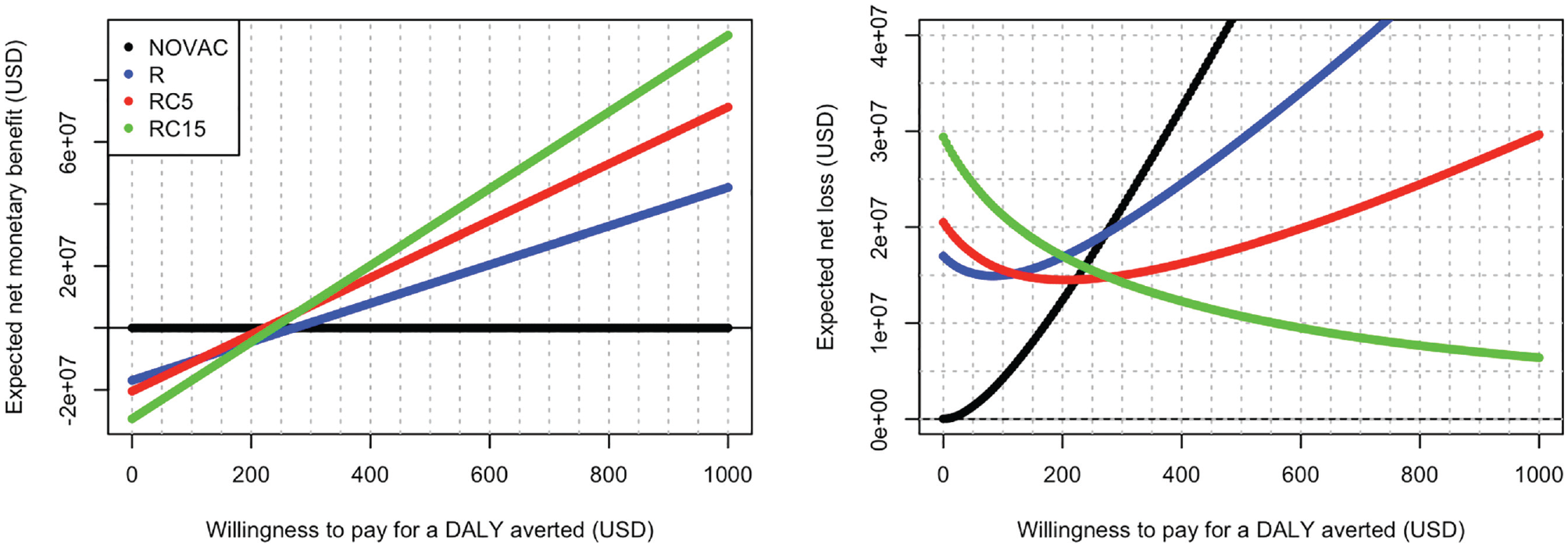
Expected incremental net monetary benefit plot (INMB plot, left) and expected net loss plot (ENL plot, right) for 4 typhoid conjugate vaccination options in Nepal: no vaccination (NOVAC), routine childhood vaccination (R), routine plus onetime catch-up campaign up to age 5 years (RC5), and routine plus one-time catch-up campaign up to age 15 years (RC15). Results based on n = 2,000 samples drawn with probabilistic sensitivity analysis. The cost-effective strategy for a given willingness-to-pay value can be read from the upper bound of the INMB curves across strategies on the INMB plot and from the ENL frontier (i.e., the lower bound of ENL curves across interventions on the ENL plot). The ENL frontier also represents the population expected value of perfect information (EVPI) with current information.

Figure 2 also shows that at k values between USD223 and USD277 per DALY averted, the distance between the expected INMB/NL lines of NOVAC and RC15 and the cost-effective intervention RC5 is rather small. Hence, if a k value between USD223 and 277 per DALY averted is considered acceptable for Nepal, no vaccination and RC15 may also be considered for implementation, with a limited lower expected INMB compared to the cost-effective intervention RC5.

What is the extent of (decision) uncertainty?

As explained above, confidence or credible intervals do not necessarily inform about the extent of decision uncertainty. Also, for this example, confidence or credible intervals cannot be constructed around the ICER because the incremental costs and effects span more than 1 quadrant. This can be seen on the cost-effectiveness plane (Figure 3): some dots show negative incremental costs, indicating cost savings. However, the cost-effectiveness plane does not show the magnitude and consequences of decision uncertainty. In this case, although ICER can be used to identify the cost-effective strategy (Table 5), INMB and NL/EVPI still need to be calculated to quantify decision uncertainty.

Figure 3

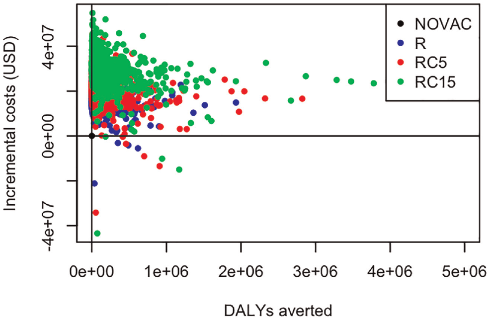
Expected incremental costs and disability-adjusted life years (DALYs) averted for 4 typhoid conjugate vaccination options in Nepal: no vaccination (NOVAC), routine childhood vaccination (R), routine plus onetime catch-up campaign up to age 5 years (RC5), and routine plus one-time catch-up campaign up to age 15 years (RC15). For each intervention, 2,000 dots are shown representing n = 2,000 samples drawn with probabilistic sensitivity analysis.

Confidence or credible intervals cannot be constructed around the INMB, because in this example, more than 2 interventions are compared. The probability that each intervention is cost-effective can be calculated and is best presented as CEACs for a range of k values (Figure 4, left plot). The cost-effectiveness acceptability frontier indicates the cost-effective intervention for each k value (Figure 4, left plot, crosses). RC5 is the cost-effective intervention for Nepal for a k between USD223 and USD277 per DALY averted.

Figure 4

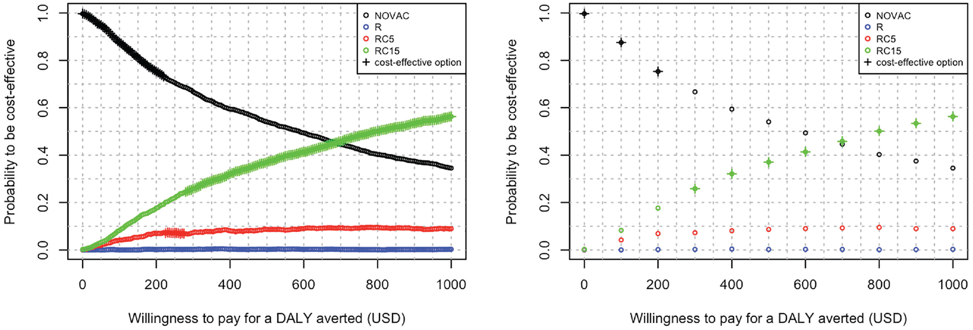
Probability to be cost-effective for 4 typhoid conjugate vaccination options in Nepal: no vaccination (NOVAC), routine childhood vaccination (R), routine plus onetime catch-up campaign up to age 5 years (RC5), and routine plus onetime catch-up campaign up to age 15 years (RC15). Probability to be cost-effective and cost-effective option (crosses) is evaluated for 201 (left plot) and 11 (right plot) equidistant willingness-to-pay (k) values. Results based on n = 2,000 samples drawn with probabilistic sensitivity analysis. DALY, disability-adjusted life year.

This example first illustrates the importance of evaluating INMB for k values close enough to each other. Figure 4 (right plot) shows the results of evaluating only 11 equidistant k values between USD0 and USD1,000 per DALY averted. This would not reveal that RC5 is the cost-effective strategy for a small range of k values, because INMB values for k between USD200 and USD300 are not evaluated (i.e., in Figure 4 [right plot], RC5 is not marked as the cost-effective strategy).

Second, Figure 4 and Table 6 show that for a k value of USD250 per DALY averted, RC5 has only a 7.25% probability to be cost-effective, much less than NOVAC (70.60%) and RC15 (21.95%). In other words, there is a 93% (1 – 0.0725 = 0.9275) probability that RC5 is not cost-effective. This is an example of how showing only CEACs (without the cost-effectiveness acceptability frontier) can be misleading, as readers could wrongly conclude RC15 is cost-effective for k values of USD700 or more, and RC5 is never cost-effective. Even when also CEAF is plotted, readers could wrongly interpret that the cost-effective option is most uncertain at a k of USD700 per DALY averted, because the probability to be cost-effective for both NOVAC and RC15 lies below 50%, whereas at a k of USD 250 per DALY averted, the probability to be cost-effective for NOVAC is 70%. This is because CEACs do not show the consequences of decision uncertainty.

Table 6

Probability to Be Cost-Effective, Expected Net Loss When Not Cost-Effective, and Expected Net Loss for 4 Typhoid Conjugate Vaccination Options in Nepal: No Vaccination (NOVAC), Routine Childhood Vaccination (R), R plus Onetime Catch-up Campaign up to Age 5 Years (RC5), and R plus Onetime Catch-up Campaign up to Age 15 Years (RC15).^a

	Probability to Be Cost-Effective (i)	Expected Net Loss of Subset of n Samples for Which Intervention Is Not Cost-Effective (ii), USD	Expected Net Loss (Averaged Over All n Samples) = (1 – (i)) * (ii), USD
NOVAC	0.7060	USD 58,242,215	USD 17,123,211
R	0.0020	USD 18,541,316	USD 18,504,233
RC5	0.0725	USD 15,775,694	USD 14,631,915
RC15	0.2195	USD 19,865,554	USD 15,505,065

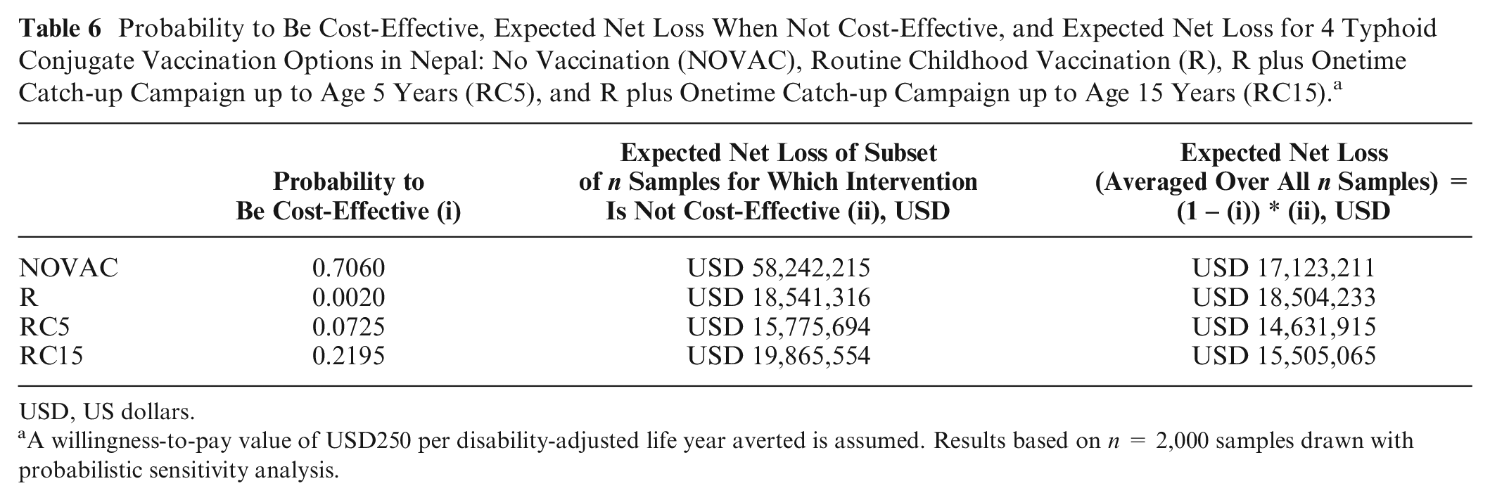
USD, US dollars.

A willingness-to-pay value of USD250 per disability-adjusted life year averted is assumed. Results based on n = 2,000 samples drawn with probabilistic sensitivity analysis.

The consequence of choosing RC5 anyway (i.e., the average of the net loss for only the samples where the intervention is not cost-effective) amounts to USD15.8 million for a k value of USD250 per DALY averted (Table 6, third column). If we would choose not to implement a vaccination program, there would be only a 30% probability to be wrong, but the cost in terms of expected net loss amounts to more than USD58 million (Table 6, third column). Expected NL for an intervention can be calculated alternatively as the probability to be cost-effective times the expected NL for the samples where the intervention is not cost-effective (Table 6, fourth column). Hence, this explains why the expected NL (net loss averaged over all n samples) for RC5 is smaller than for the other strategies and why consequently, RC5 is the cost-effective strategy for k being USD250 per DALY averted. Expected NL also explains why for this example decision uncertainty is largest at k being USD250 per DALY averted and not at k being USD700 per DALY averted.

For Nepal, decision uncertainty is highest at k values between USD200 and USD300 per DALY averted (Figure 2, expected NL of cost-effective strategy is highest for k values between USD200 and USD300). This is where the cost-effective intervention changes from NOVAC to RC5 to RC15 with increasing k value. If Nepal would be willing to pay around USD250 for a DALY averted, population EVPI given current information is USD14.6 million (population EVPI because it is calculated for the complete target group [9-month-old children + catch-up age group] over a time horizon of 30 years). If the cost to design and conduct studies to estimate all 24 uncertain input parameters of this typhoid cost-effectiveness model precisely is less than USD14.6 million, investing in these studies may be justified. However, to “know” if further research is worthwhile, additional analyses, requiring additional data and assumptions, are needed. Note that EVPI depends on k: if Nepal would be willing to pay USD750 per DALY averted, population EVPI is less than USD10 million.

With the results of the current model, also population-level current EVPPI values can be obtained for each of the 24 uncertain input parameters. Figure 5 shows that the uncertainty around the probability to be hospitalized for typhoid fever induces most decision uncertainty (black solid line). Studies that cost up to USD10 million (= population EVPPI value at USD250 per DALY averted for the hospital probability) could be justified to measure more precisely the probability to be hospitalized when having typhoid fever, in order to determine the cost-effectiveness intervention with more certainty.

Figure 5

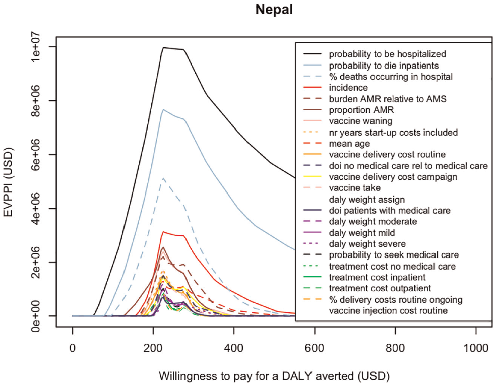
Expected value of partial perfect information (EVPPI) for the target population over a time horizon of 30 years (population EVPPI given current information) for 24 uncertain input parameters for a range of willingness-to-pay (k) values. Parameter names in legend are ordered according to decreasing EVPPI values. Results based on n = 2,000 samples drawn with probabilistic sensitivity analysis.

Second most influential are the uncertainties around the probability to die if hospitalized (solid light-blue line), the percentage of typhoid-related deaths occurring in hospitalized patients (dashed light-blue line), and the overall typhoid incidence (solid red line). These have the highest population EVPPI values for the k values considered.

Note that if Nepal would be willing to pay only USD50 per DALY averted, much less decision uncertainty exists (population EVPI or expected net loss is less than USD1.3 million; Figure 2). At a k value of USD50 per DALY averted, the population EVPPI of the probability to be hospitalized would drop to USD14,815 and the population EVPPI values of all 23 other uncertainties input parameters would be USD0. Hence, if Nepal would be willing to pay USD50 per DALY averted, no vaccination would be the cost-effective strategy, and a future study to measure hospital probability precisely would have to cost below USD14,815 to be justified.

Summary

The (most) cost-effective health care intervention from a set of interventions is the intervention that is on average cost-effective, irrespective of the degree of uncertainty. It can be identified either by 1) applying concepts of dominance and extended dominance in combination with calculating expected ICERs (as a ratio of means), 2) calculating expected INMB or INHB and choosing the intervention resulting in the highest expected INMB or INHB, or, equivalently, 3) calculating expected NL and choosing the intervention resulting in the lowest expected NL (Figure 1). The current best measure for decision uncertainty is the EVPI, which is equal to the expected NL when choosing the cost-effective intervention. The cost-effective intervention and the extent of decision uncertainty depend on the cost-effectiveness (“willingness-to-pay”) threshold k. Perhaps the most informative plot to present key cost-effectiveness results is the expected NL curves plot, as it shows the cost-effective intervention, how much better it is compared to alternatives, and the EVPI for a range of k values. Appendix 3.3 provides R code for an example of comparing more than 2 interventions with uncertainty, covering all calculations and all plots mentioned in this tutorial.

Discussion

This tutorial describes with an easy-to-use flowchart how to identify the cost-effective intervention from a range of alternatives and how to best present these results, depending on the number of alternatives compared and on whether uncertainty was quantified in a probabilistic way. It also covers how to estimate and interpret decision uncertainty. This tutorial adds on existing guidelines as it 1) compares all currently available approaches in how they can answer the same questions and 2) covers both “what to do” as well as “how to do” (i.e., with examples and R code). We hope this tutorial will improve the correct generation and interpretation of health economic evaluation results and, consequently, health care decision making.

This tutorial describes the use of the expected cost-effectiveness to determine the intervention of choice from a set of alternatives. This decision rule assumes that decision makers are risk neutral, that decisions are reversible (with no associated costs), and that no cost of evidence foregone exists.^30,31 Some have argued that these assumptions do not hold, and therefore other decision rules have been proposed.³² However, if the aim is to maximize health gain for a given budget, health care strategies should be chosen based on expected cost-effectiveness, irrespective of the degree of uncertainty.^1,12

The role of accounting for uncertainty is to estimate this expected cost-effectiveness correctly and to decide if current evidence is enough to take a decision now and if investing in research is valuable.³¹ However, in practice, it is often not straightforward to assess if further research is worthwhile, as this requires additional information (e.g., cost of research to calculate EVSI and ENBS). Obtaining EVPI and EVPPI values is much easier (i.e., by applying available approximation methods to the PSA sample of a health economic evaluation).^33,34 Although EVPI values do not answer the question if more research is valuable, they do provide useful information for guiding decision making. In particular, EVPPI values indicate which uncertainties impact most on decision uncertainty.

Although not covered in this tutorial, we believe sensitivity analysis should form part of any health economic evaluation. Techniques like 1-way and multiway sensitivity analysis and variable importance measures for individual uncertain parameters can help understand a model. Scenario analysis and multimodel comparisons can be used to investigate the impact on results of uncertainties that are not quantified in a probabilistic way (e.g., different methodological choices or model structures).^24,35–37 Note that both the cost-effective intervention as well as the extent of decision uncertainty can depend on the scenarios and/or models used.

This tutorial focused on some of the key benefits and limitations of the different cost-effectiveness measures and plots; for more in-depth discussion of broader benefits, see Eckermann²⁰ (NL) and Paulden³⁸ and O’Mahony³⁹ (ICER and INMB).

Correct application of the methods described in this tutorial does not guarantee correct cost-effectiveness results. This tutorial starts from the costs and effects for each intervention considered and hence assumes that all prior steps have been done appropriately. This includes setting the methodological framework, incorporating all plausible options for intervention, choosing the appropriate model, and estimating all model input parameters and their uncertainty correctly.^12,40

Importantly, many criteria other than cost-effectiveness are involved in health care decision making, such as equity, feasibility, and budget impact.⁴¹ Hence, decision makers may not always choose to adopt the technology that maximizes expected net benefit. Nevertheless, cost-effectiveness information provided to decision makers should be reliable, and therefore the best available methods should be used in the correct way.

We hope this tutorial facilitates the (correct) use of existing methods in applied health economic evaluations to identify the cost-effective intervention among a set of alternatives and the associated uncertainty. By updating local guidelines,¹⁰ health economists could be further encouraged to adopt these methods.

Supplemental Material

sj-docx-1-mdm-10.1177_0272989X211045070 – Supplemental material for Generating, Presenting, and Interpreting Cost-Effectiveness Results in the Context of Uncertainty: A Tutorial for Deeper Knowledge and Better Practice

Supplemental material, sj-docx-1-mdm-10.1177_0272989X211045070 for Generating, Presenting, and Interpreting Cost-Effectiveness Results in the Context of Uncertainty: A Tutorial for Deeper Knowledge and Better Practice by Joke Bilcke and Philippe Beutels in Medical Decision Making

Footnotes

Acknowledgements

This tutorial benefited from discussions with members of the CHERMID group. We thank the reviewers and editors for their valuable comments.

The author(s) declared no potential conflicts of interest with respect to the research, authorship, and/or publication of this article.

The author(s) disclosed receipt of the following financial support for the research, authorship, and/or publication of this article: Financial support for this study was provided in part by a grant from the Scientific Research Foundation–Flanders. The funding agreement ensured the authors’ independence in designing the study, interpreting the data, writing, and publishing the report. The following author is employed by the sponsor: JB (postdoctoral fellowship).

ORCID iDs

Joke Bilcke

Philippe Beutels

Supplemental Material

Supplementary material for this article is available on the Medical Decision Making website at .

References

Claxton

The irrelevance of inference: a decision-making approach to the stochastic evaluation of health care technologies. J Health Econ. 1999;18(3):341–64.

Groot Koerkamp

Hunink

Stijnen

Hammitt

Kuntz

Weinstein

. Limitations of acceptability curves for presenting uncertainty in cost-effectiveness analysis. Med Decis Making. 2007;27(2):101–11.

O’Mahony

Paulden

Appraising the cost-effectiveness of vaccines in the UK: insights from the Department of Health Consultation on the revision of methods guidelines. Vaccine. 2019;37(21):2831–7.

Cleemput

Neyt

Van de Sande

Thiry

. Belgian Guidelines for Economic Evaluations and Budget Impact Analyses. 2nd ed. Health Technology Assessment (HTA). Brussels: Belgian Health Care Knowledge Centre (KCE); 2012. KCE Report 183C. D/2012/10.273/54

Stinnett

Mullahy

Net health benefits: a new framework for the analysis of uncertainty in cost-effectiveness analysis. Med Decis Making. 1998;18(2):S68–S80.

Fenwick

Briggs

Cost-effectiveness acceptability curves in the dock: case not proven?

Med Decis Making. 2007;27(2):93–5.

Eckermann

Willan

AR.

Presenting evidence and summary measures to best inform societal decisions when comparing multiple strategies. Pharmacoeconomics. 2011;29(7):563–77.

Eckermann

Briggs

Willan

AR.

Health technology assessment in the cost-disutility plane. Med Decis Making. 2008;28(2):172–81.

Guideline for Economic Evaluations in Healthcare . Netherlands, Diemen: National Health Care Institute; 2016.

10.

Guidelines for the Economic Evaluation of Health Technologies: Canada . 4th ed. Ottawa: CADTH; 2017.

11.

Alarid-Escudero

Enns

Kuntz

Michaud

Jalal

. “Time traveling is just too dangerous” but some methods are worth revisiting: the advantages of expected loss curves over cost-effectiveness acceptability curves and frontier. Value Health. 2019;22(5): 611–18.

12.

Drummond

Sculpher

Claxton

Stoddart

Torrance

. Methods for the Economic Evaluation of Health Care Programmes. 4th ed. New York: Oxford University Press; 2015.

13.

Ryen

Svensson

The willingness to pay for a quality adjusted life year: a review of the empirical literature. Health Econ. 2015;24(10):1289–301.

14.

Karlsson

Johannesson

The decision rules of cost-effectiveness analysis. Pharmacoeconomics. 1996;9(2):113–20.

15.

Thokala

Ochalek

Leech

Tong

. Cost-effectiveness thresholds: the past, the present and the future. Pharmacoeconomics. 2018;36(5):509–22.

16.

Bertram

Lauer

De Joncheere

Edejer

Hutubessy

Kieny

, et al. Cost-effectiveness thresholds: pros and cons. Bull WHO. 2016;94(12):925–30.

17.

Stinnett

Paltiel

AD.

Estimating CE ratios under second-order uncertainty: the mean ratio versus the ratio of means. Med Decis Making. 1997;17(4):483–9.

18.

Johannesson

Weinstein

MC.

On the decision rules of cost-effectiveness analysis. J Health Econ. 1993;12(4):459–67.

19.

Cantor

SB.

Cost-effectiveness analysis, extended dominance, and ethics: a quantitative assessment. Med Decis Making. 1994;14(3):259–65.

20.

Eckermann

Health Economics from Theory to Practice. Cham, Switzerland: Springer International Publishing AG; 2017.

21.

Briggs

Goeree

Blackhouse

O’Brien

. Probabilistic analysis of cost-effectiveness models: choosing between treatment strategies for gastroesophageal reflux disease. Med Decis Making. 2002;22(4):290–308.

22.

van Hout

Gordon

Rutten

. Costs, effects and C/E-ratios alongside a clinical trial. Health Econ. 1994;3(5):309–19.

23.

Felli

Hazen

GB.

Sensitivity analysis and the expected value of perfect information. Med Decis Making. 1998;18(1):95–109.

24.

Briggs

Claxton

Sculpher

Decision Modelling for Health Economic Evaluation. New York: Oxford University Press; 2006.

25.

Eckermann

Karnon

Willan

AR.

The value of value of information: best informing research design and prioritization using current methods. Pharmacoeconomics. 2010;28(9):699–709.

26.

Black

WC.

The Ce plane—a graphic representation of cost-effectiveness. Med Decis Making. 1990;10(3):212–14.

27.

Willan

AR.

Incremental net benefit in the analysis of economic data from clinical trials, with application to the CADET-Hp Trial. Eur J Gastroenterol Hepatol. 2004;16(6):543–9.

28.

Fenwick

Claxton

Sculpher

Representing uncertainty: the role of cost-effectiveness acceptability curves. Health Econ. 2001;10(8):779–87.

29.

Bilcke

Antillón

Pieters

Kuylen

Abboud

Neuzil

, et al. Cost-effectiveness of routine and campaign use of typhoid Vi-conjugate vaccine in Gavi-eligible countries: a modelling study. Lancet Infect Dis. 2019;19(7):728–39.

30.

Griffin

Claxton

Palmer

Sculpher

. Dangerous omissions: the consequences of ignoring decision uncertainty. Health Econ. 2011;20(2):212–24.

31.

Claxton

Exploring uncertainty in cost-effectiveness analysis. Pharmacoeconomics. 2008;26(9):781–98.

32.

Basu

Meltzer

Decision criterion and value of information analysis: optimal aspirin dosage for secondary prevention of cardiovascular events. Med Decis Making. 2018;38(4):427–38.

33.

Heath

Manolopoulou

Baio

Efficient Monte Carlo estimation of the expected value of sample information using moment matching. Med Decis Making. 2018;38(2):163–73.

34.

Strong

Oakley

Brennan

Breeze

. Estimating the expected value of sample information using the probabilistic sensitivity analysis sample: a fast, nonparametric regression-based method. Med Decis Making. 2015;35(5):570–83.

35.

Walker

Fox-Rushby

Allowing for uncertainty in economic evaluations: qualitative sensitivity analysis. Health Policy Plan. 2001;16(4):435–43.

36.

Bilcke

Beutels

Brisson

Jit

. Accounting for methodological, structural, and parameter uncertainty in decision-analytic models: a practical guide. Med Decis Making. 2011;31(4):675–92.

37.

den Boon

Jit

Brisson

Medley

Beutels

White

, et al. Guidelines for multi-model comparisons of the impact of infectious disease interventions. BMC Med. 2019;17(1):163.

38.

Paulden

Why it’s time to abandon the ICER. Pharmacoeconomics. 2020;38(8):781–4.

39.

O’Mahony

JF.

Does cost-effectiveness analysis really need to abandon the incremental cost-effectiveness ratio to embrace net benefit?

Pharmacoeconomics. 2020;38(8):777–9.

40.

Husereau

Drummond

Petrou

Carswell

Moher

Greenberg

, et al. Consolidated Health Economic Evaluation Reporting Standards (CHEERS)—explanation and elaboration: a report of the ISPOR Health Economic Evaluation Publication Guidelines Good Reporting Practices Task Force. Value Health. 2013;16(2):231–50.

41.

Guindo

Wagner

Baltussen

Rindress

van Til

Kind

, et al. From efficacy to equity: literature review of decision criteria for resource allocation and healthcare decisionmaking. Cost Eff Resour Alloc. 2012;10(1):9.

Supplementary Material

Please find the following supplemental material available below.

For Open Access articles published under a Creative Commons License, all supplemental material carries the same license as the article it is associated with.

For non-Open Access articles published, all supplemental material carries a non-exclusive license, and permission requests for re-use of supplemental material or any part of supplemental material shall be sent directly to the copyright owner as specified in the copyright notice associated with the article.

0.00 MB

20.52 MB

Generating,Presenting,and Interpreting Cost-Effectiveness Results in the Context of Uncertainty: A Tutorial for Deeper Knowledge and Better Practice

Abstract

Keywords

Introduction

Basic Concepts

Measures for Cost-Effectiveness

The cost-effectiveness threshold and decision making

Answering Key Cost-Effective Questions

How to Identify the Cost-Effective Intervention?

What is the cost-effective option from 2 interventions when no uncertainty is accounted for?

What is the cost-effective option from more than 2 interventions when no uncertainty is accounted for?

What is the cost-effective intervention when uncertainty is accounted for in a probabilistic way?

How to Measure and Interpret the Extent of Decision Uncertainty Surrounding the Cost-Effective Results?

How to Report or Present Main Cost-Effectiveness Results?

Real-Life Example of Generating, Presenting, and Interpreting Cost-Effectiveness Results

What is the cost-effective intervention?

What is the extent of (decision) uncertainty?

Summary

Discussion

Supplemental Material

sj-docx-1-mdm-10.1177_0272989X211045070 – Supplemental material for Generating, Presenting, and Interpreting Cost-Effectiveness Results in the Context of Uncertainty: A Tutorial for Deeper Knowledge and Better Practice

Footnotes

Acknowledgements

ORCID iDs

Supplemental Material

References

Supplementary Material