Sage Journals: Discover world-class research

Abstract

Objectives. Uncertainty in survival prediction beyond trial follow-up is highly influential in cost-effectiveness analyses of oncology products. This research provides an empirical evaluation of the accuracy of alternative methods and recommendations for their implementation. Methods. Mature (15-year) survival data were reconstructed from a published database study for “no treatment,” radiotherapy, surgery plus radiotherapy, and surgery in early stage non–small cell lung cancer in an elderly patient population. Censored data sets were created from these data to simulate immature trial data (for 1- to 10-year follow-up). A second data set with mature (9-year) survival data for no treatment was used to extrapolate the predictions from models fitted to the first data set. Six methodological approaches were used to fit models to the simulated data and extrapolate beyond trial follow-up. Model performance was evaluated by comparing the relative difference in mean survival estimates and the absolute error in the difference in mean survival v. the control with those from the original mature survival data set. Results. Model performance depended on the treatment comparison scenario. All models performed reasonably well when there was a small short-term treatment effect, with the Bayesian model coping better with shorter follow-up times. However, in other scenarios, the most flexible Bayesian model that could be estimated in practice appeared to fit the data less well than the models that used the external data separately. Where there was a large treatment effect (hazard ratio = 0.4), models that used external data separately performed best. Conclusions. Models that directly use mature external data can improve the accuracy of survival predictions. Recommendations on modeling strategies are made for different treatment benefit scenarios.

Keywords

external data extrapolation health technology assessment survival analysis

Survival analysis has become an important part of cost-effectiveness methods for health technology appraisals. Current health technology assessments usually require mean survival times to estimate the life years gained or, for Markov models, transition probabilities per cycle. Mean survival times are typically derived from fitting parametric survival curves for the lifetime of patients and the integral of the fitted survival curve used to estimate mean survival. However, early in their training, statisticians are warned against extrapolating statistical relationships past the range of observed data.¹ Survival models can produce meaningfully different mean overall survival times even when they show little differentiation in model fit.² Davies et al.³ provide evidence of changing hazard rates over time and discuss the associated bias if only short-term data are used to predict long-term survival. The current National Institute for Health and Care and Excellence (NICE) Decision Support Unit (DSU) guidelines⁴ place an emphasis on choosing models by considering internal and external validity and conducting sensitivity analyses with alternative plausible models. NICE⁵ requires several alternative scenarios reflecting different assumptions about future treatment effects, which typically include the assumption that treatment does not provide further benefit beyond the treatment period as well as more optimistic assumptions. However, there is no guarantee that any model, even the best-fit model, will give accurate predictions of the future.^2,6

Alternative approaches to survival curve extrapolation include model-averaging techniques,^7–9 hybrid models,^10,11 Bayesian poly-Weibull models,^12,13 cure models,¹⁴ and combination of trial and external data.^15,16 The need for long-term data to perform survival curve extrapolation has been expressed.^15–17 Despite the number of methods in the literature, little work has been conducted to assess how reliable survival predictions are compared to actual or simulated long-term data.

The aim of this article was to evaluate the performance of a range of models under different scenarios and make recommendations on how to choose an appropriate analytical strategy for future projects. To achieve this aim, a long-term published data set was identified in early stage non–small cell lung cancer (NSCLC) in elderly patients. The data contain 15.5 years of follow-up and represent complete survival estimates for 4 treatments. These data contained examples of 3 scenarios that are commonly found in data from randomized controlled trials (RCTs):

Small short-term benefit of treatment effect (radiotherapy)

Small long-term benefit of treatment effect (surgery plus radiotherapy)

Large long-term benefit of treatment effect (surgery)

From these data, pseudo-short-term trial data sets were created. Six different approaches were used to fit survival models and perform the extrapolation, 4 of which made use of long-term external data. Performance of these models was assessed using relative error of mean survival estimates and absolute error for difference in mean survival v. the control by comparing predicted mean overall survival distributions to those derived from Kaplan-Meier estimates from bootstrapped samples from the complete data set. Extrapolated long-term survival curves, mean survival distributions, and sensitivity analyses are presented. Finally, the findings and limitations of these methods are discussed.

Despite this research being based on observational data, it is expected that the results and conclusions will be relevant to the problems associated with survival curve extrapolation from RCTs.

Methods

Observational Treatment Comparison Data

Ganti et al.¹⁸ present Kaplan-Meier estimates separately for stage I and II NSCLC for an elderly population (≥80 years old) derived from Surveillance, Epidemiology, and End Results (SEER) data for patients diagnosed between 1998 and 2007. Kaplan-Meier estimates were presented for no treatment (n = 343), radiotherapy (n = 346), surgery in combination with radiotherapy (n = 55), and surgery alone (n = 594). The data contained some observed differences in survival between treatment arms that cannot be ascribed directly to treatment effects, as there may be confounding by severity in assignment to different treatment arms (e.g., percentage of stage II cancer: no treatment, 15%; radiation, 20%; surgery, 13%; surgery in combination with radiotherapy, 44%). Only patients who were deemed fit to undergo surgery by clinicians underwent resection. There was also an increasing trend during the study period of patients opting for no treatment.¹⁸

The data were digitized and reconstructed following the methods described by Guyot et al.¹⁹ Kapan-Meier estimates from the reconstructed data are presented in the online appendix (Suppl. Figure S1). This chart shows a steep drop from 0 to 1 month for the no-treatment arm and high survival probability for the surgery plus radiotherapy arm. This result may be due to the data being observational and the possibility that some patients may have died before the intended treatment started or that patients may have had a short life expectancy and did not receive any treatment. Conversely, the fittest patients may have been considered suitable for radiotherapy plus surgery. A sudden drop in survival at the start of a study is rarely observed in oncology trials, as they typically have an inclusion criterion that patients have a life expectancy of 3 months. To mimic a trial in which such patients would likely not be included, 1 month was subtracted from patients’ survival times in all treatment arms and records with a negative time removed from the data. The resulting Kaplan-Meier estimates are presented in Figure 1 (color version is provided in the online appendix). The overall hazard ratios, 95% confidence intervals (CIs), and P values from this data set were radiotherapy (0.92 [0.79–1.08]; P = 0.334), surgery plus radiotherapy (0.70 [0.52–0.93]; P = 0.015), and surgery (0.37 [0.32–0.44]; P < 0.0001). Smoothed hazard rates and hazard ratios estimated from these data are presented in the online appendix (Suppl. Figure S2 and Suppl. Figure S3, respectively). The hazard rates and hazard ratios were observed to change over time. In particular, the hazard rates for radiotherapy showed a significant increase followed by a significant decrease, and the hazard rates for surgery alone showed a significant increase during the follow-up time. The hazard ratios for surgery showed a significant change v. no treatment, remaining close to 0.4 for the first 3 years and changing to be close to 0.8 from 5.5 years.

Figure 1

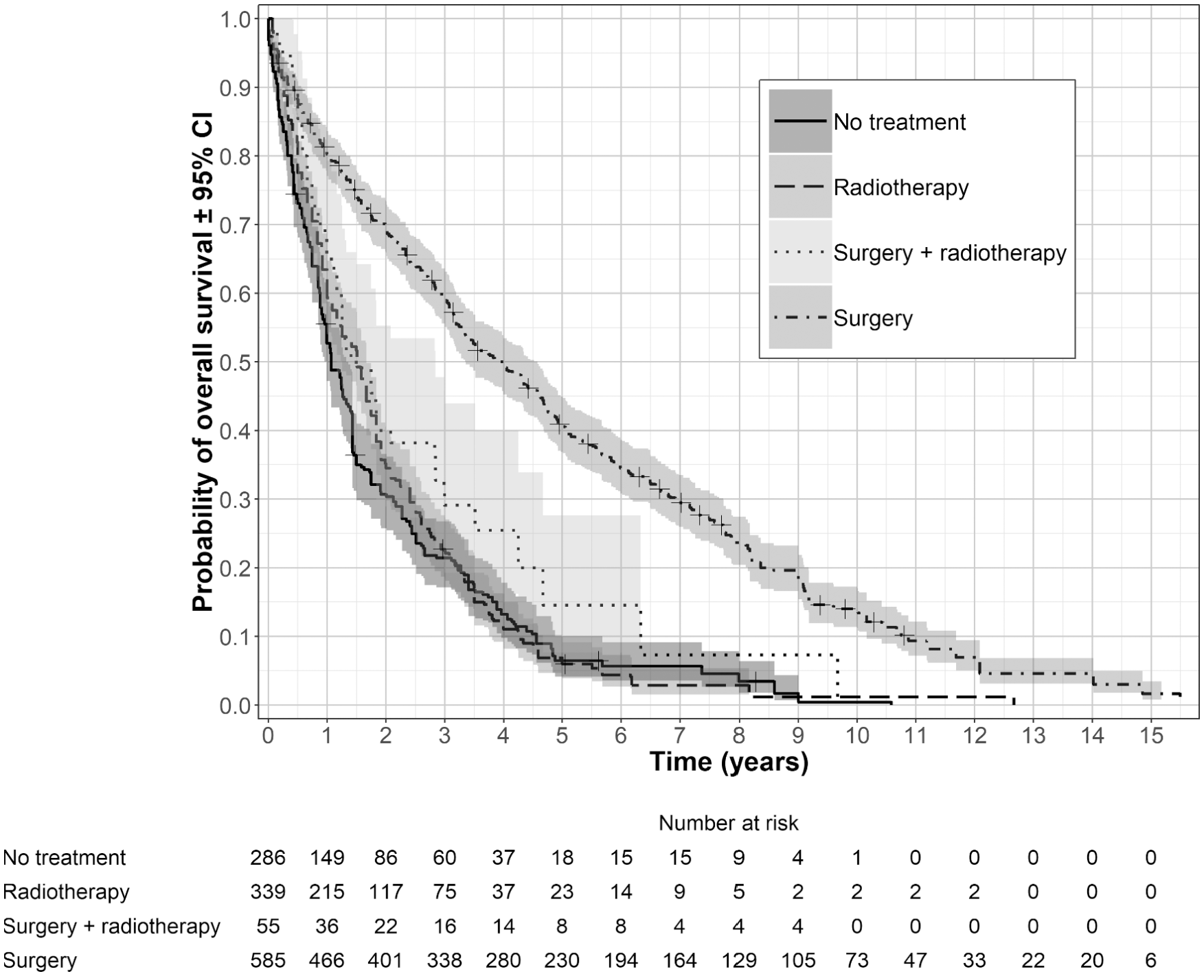
Data presented by Ganti et al.¹⁸ for early stage non–small cell lung cancer in elderly patients after removal of the first month of data from all treatment arms.

It was assumed that patients could enter the trial at any time point in the first 12 months (assuming a uniform distribution) and that patients survived according to the data presented in Figure 1. The data were cut at 1 to 10 years at annual intervals, with patients still alive censored at the end of each cut point. Kaplan-Meier estimates for each cut point are presented in the online appendix (Suppl. Figure S4).

Disease-Specific External Data

A common problem of using external data to aid extrapolation is that data from a different source will not match the trial population exactly. The treatments used are likely to represent a broader range of treatment options, and although patients may have similar disease characteristics, they are likely to be from different geographical areas and/or have a broader range of characteristics. Also, because the data are longer term, they represent patients who started treatment further back in time when the standard of care may have been different to that observed during the trial. A search of the literature was conducted to identify an additional long-term data set. The closest found was that presented by Bach et al.²⁰

Bach et al.²⁰ present Kaplan-Meier estimates for black and white patient populations with stage I and II NSCLC who were ≥65 years old and were diagnosed between 1985 and 1993 (n = 2,589). These data were reconstructed using the method described by Guyot et al.¹⁹ One month was subtracted from survival times, and records with negative values were removed, to match the data from Ganti et al.¹⁸ The Kapan-Meier estimates from the reconstructed data are presented in Figure 2A. These data were matched to the no-treatment data presented by Ganti et al.¹⁸ by fitting accelerated failure time models (Weibull, generalized gamma, log-normal, log-logistic) and applying the time acceleration factor (multiply/divide original time values by the time acceleration factor²¹) from the best-fitting model (Weibull) to the Bach et al.²⁰ data. Survival times that exceeded the maximum follow-up time from Bach et al.²⁰ were censored at that time point. Figure 2B presents this adjustment for the complete data set. This procedure was repeated for each cut point; the resulting time acceleration factors for each cut point are presented in Figure 2C. These data appeared to contain little information on general mortality, so a further extrapolation was needed using general population data. A comparison of the hazard rates and hazard ratios from the complete data presented by Ganti et al.¹⁸ and the time-accelerated adjusted data presented by Bach et al.²⁰ (with the first month of data removed) is presented in the appendix (Suppl. Figure S5 and Suppl. Figure S6, respectively). There was good agreement in these predictions for a follow-up of up to 6 years.

Figure 2

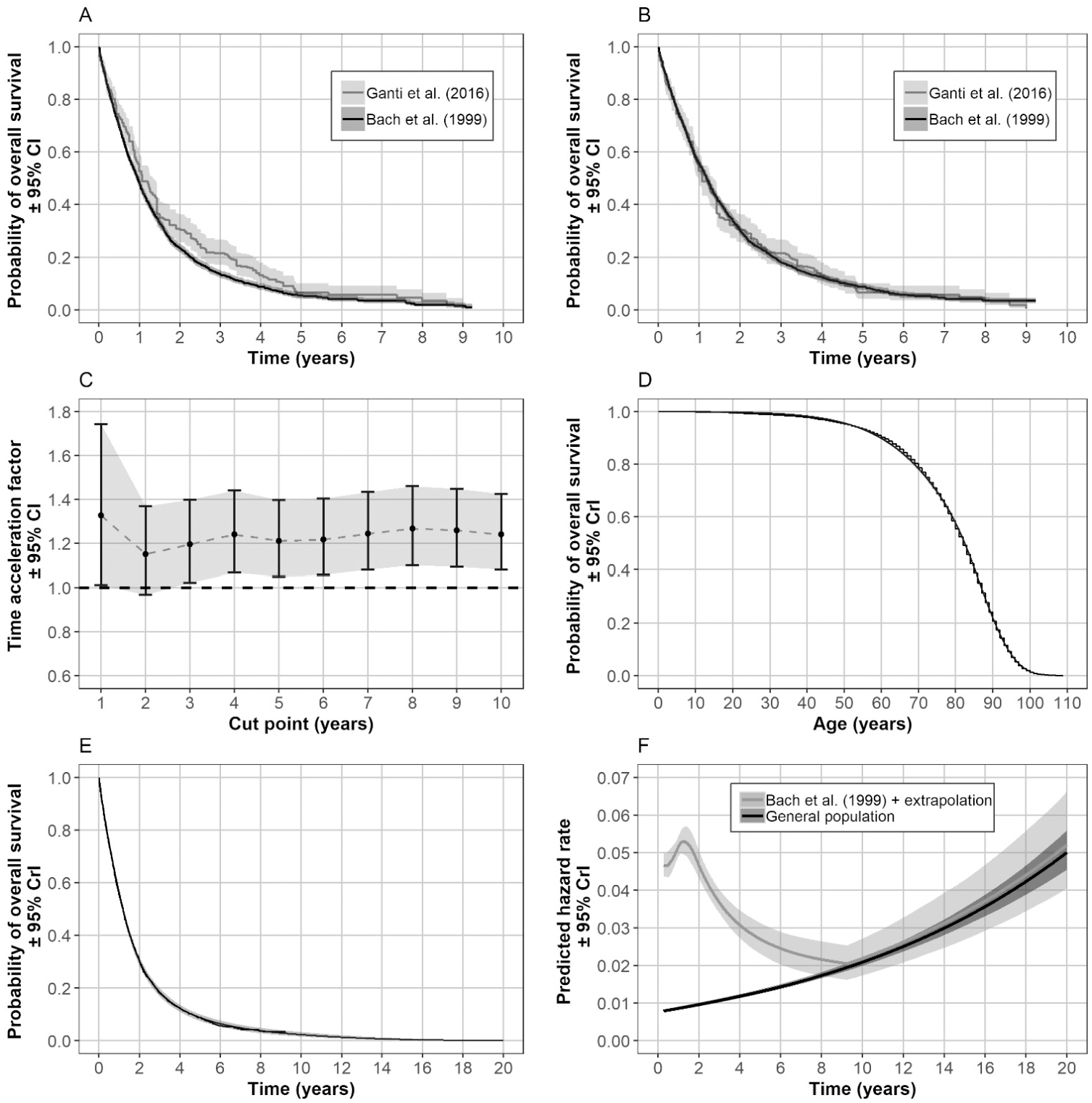
Steps involved in estimating the hazard rates from disease-specific external data and general population data for the no-treatment arm for each cut point. Original reconstructed data for no treatment (A). Bach et al.²⁰ data adjusted using a time acceleration factor to match the data presented by Ganti et al.¹⁸ (B). Check that time acceleration factor was consistent across cut points (C). Royston and Parmer²⁴ spline model fitted to the general population data after removal of infant mortality (<3 years) (D). Royston and Parmer²⁴ spline model fitted to the adjusted data presented by Bach et al.,²⁰ with extrapolation based on hazard ratio–adjusted predictions from the model fitted to general population data (E). Predicted hazard rates for the external data derived from the model presented in chart (E) and after follow-up (9 years) from the adjusted hazard rates from the general population data (F). CI, confidence interval; CrI, credible interval.

General Population Data

Bell and Miller²² present general population life table data for a cohort of 100,000 patients in the United States. These were reconstructed for 10,000 individuals using the methods described by Guyot et al.¹⁹ and were weighted according to sex for patients ≥80 years old from data presented by Howden and Meyer.²³ The Kaplan-Meier estimates and best-fitting model (Royston and Parmar²⁴ spline model with 3 knots assuming proportional hazards) predictions are presented in Figure 2D.

Model to Extrapolate the Disease-Specific External Data Using the General Population Data

Parametric models with a proportional hazard property (Weibull, Gompertz, and Royston and Parmar²⁴ spline models with 1–4 knots assuming proportional hazards) were fitted to the time-accelerated adjusted data from Bach et al.²⁰ The Royston and Parmar²⁴ spline model with 3 knots gave the best fit according to both Akaike information criterion (AIC) and Bayesian information criterion (BIC). The hazard rates were used to the end of follow-up for these data; then after this time point, predicted hazard rates were derived from the model fitted to the general population data for an age distribution (half normal) that matched patients ≥80 years of age (plus the follow-up time) according to Howden and Meyer.²³ The hazard ratio was estimated for the external data at end of follow-up v. the general population data, and this was applied to the predicted hazards from the external data to give a seamless transition between the 2 models. The resulting survival curve is presented in Figure 2E and the predicted hazard rates are presented in Figure 2F.

Reference Model for Complete Data Set

Kaplan-Meier estimates derived from bootstrapped data (random sample with replacement²⁵) and mean survival distributions are presented in the online appendix (Suppl. Figure S7). Predicted mean survival times were estimated as the area under each of 1000 bootstrap-predicted curves based on natural spline-based integration with 0.25-month intervals and a time horizon of 100 years (a trapezoid method gave virtually identical results).

Models Fitted to the Short-Term Observational Treatment Comparison Data Sets

The following models were fitted to the short-term observational data sets:

Most plausible parametric model (Latimer⁴)

Most plausible parametric model with external data extrapolation

Bootstrapped hybrid model (adapted from Gelber et al.¹⁰ and Bagust and Beale¹¹)

Bootstrapped hybrid model with external data extrapolation

Ensemble of parametric models with external data extrapolation

Bayesian simultaneous flexible spline–based model that used the short-term trial data and survival predictions based on the models fitted to the external and general population data (adapted from Guyot et al.¹⁵)

For each model, survival probabilities were estimated at 0.25-month intervals with a time horizon of 100 years for 1000 bootstrap or simulated values, depending on the method. External data extrapolation followed the hazard ratio tapering method described below.

Most plausible parametric model

The following parametric models were fitted to the short-term data sets: exponential, nonstratified generalized gamma, and stratified and nonstratified Weibull, Gompertz, log-normal, log-logistic, and Royston and Parmar²⁴ spline models with 1 to 3 knots. Stratified models allowed all parameters to vary by treatment. The validity of the models was assessed by comparing predictions for all time points in common to those from the external data of Bach et al.,²⁰ determining whether predictions were biologically plausible given the age of patients and, if needed, using model fit statistics from the short-term data (AIC and BIC).

Bootstrapped hybrid model

Bootstrap samples were created from the short-term data sets for each study arm. For each sample, the cumulative hazard rates were estimated and a Chow breakpoint test²⁶ used to determine the time point that explained the most variation in the change in slope. This was restricted to be less than or equal to half the follow-up time. For each bootstrap sample in which time points were less than the cut point, Kaplan-Meier estimates were used, after the cut point parametric models (exponential, Weibull, log-normal, and log-logistic) were fitted. The validity of the models was assessed by comparing predictions for all time points in common with those from the external data of Bach et al.,²⁰ determining biological plausibility of the predictions, and, if needed, using the proportion of times each parametric part of the model gave the best fit according to AIC and BIC.

Ensemble of parametric predictions with external data

This method was based on one of the methods reviewed by Jackson et al.¹⁶ The same range of models used to find the most plausible parametric model was fitted to the short-term data sets. Survival predictions were created from an ensemble of models based on the mean of Akaike weights and Bayesian weights derived from AIC and BIC values.^27–30 Survival predictions were sampled from each of the 1000 simulations to reflect these weights. The hazard rates from the models fitted to the disease-specific external data and general population data described in Figure 2 were used after the follow-up for the no-treatment arm data. For the other treatments, these hazard rates were also used, but hazard ratio tapering was applied.³¹

Extrapolation using external data and hazard ratio tapering

From the end of follow-up, of the short-term data, the hazard rates from the model fitted to the external data and general population data were used for the no-treatment arm. For the other treatments, hazard ratio tapering was applied to these hazard rates.

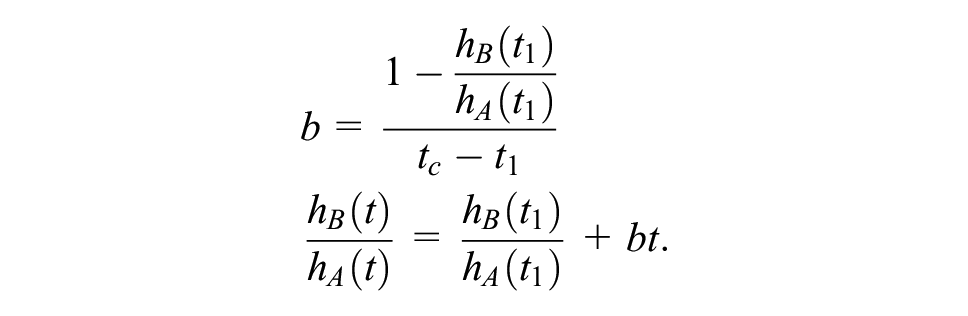
When the treatment effect was expressed as a hazard ratio of the hazard rates (h) for the control (A) and treatment under investigation (B), h_B(t)/h_A(t), the effect for time after follow-up (t > t₁) was assumed to diminish over time, and thus h_B(t)/h_A(t) increased or decreased to 1 at time t_c.

If t≤t₁, then hazard rates were estimated directly from the trial. For the control, if t > t₁, hazard rates were estimated from the external data. For the other treatments, if t > t₁ and t < t_c, a linear equation was used to estimate the hazard ratio from time t₁ to t_c (= 1) relative to the control as follows:

\begin{matrix} b = \frac{1 - \frac{h_{B} (t_{1})}{h_{A} (t_{1})}}{t_{c} - t_{1}} \\ \frac{h_{B} (t)}{h_{A} (t)} = \frac{h_{B} (t_{1})}{h_{A} (t_{1})} + bt . \end{matrix}

The time t_c was derived from simulated values from a normal distribution with a mean (µ) of 10 years and standard deviation (σ) of 2 years:

t_{c} ~ N (μ, σ^{2}) .

This formula resulted in a distribution with a range of approximately 3 to 17 years. This distribution reflected a belief that the treatment effect may continue a long time after patients received treatment but that the upper limit of the distribution could not exceed the plausible limit imposed by age. The time point of 10 years also reflected the approximate time that the hazard rates from the general population exceeded those predicted from the external data. After time t_c, hazard rates, for all treatment arms, were derived from the external data.

Bayesian simultaneous flexible spline–based model

The Bayesian simultaneous model described by Guyot et al.¹⁵ was adapted to reflect the more readily available data used in this study. For the external data, the numbers of patients alive and at risk at annual time points were derived from the predicted survival probability from the model fitted to the disease-specific external data and general population data shown in Figure 2E multiplied by the number of patients at the start of the study (2589). The Guyot model assumes that the conditional survival for the reference treatment is likely to converge to that observed in the external data after follow-up. It was assumed that the 1-year conditional survival for patients in the no-treatment arm from the short-term comparative treatment data at time t conditional on being alive at time (t – 1)—CS₀, (t |t– 1), where CS₀ is the survival probability from the short-term comparative data—is no different from the time-accelerated external population data, CS_ext(t |t– 1), from ℕ≥t₁ years onward until time ℕ_tend, where ℕ is the whole number sequence of years from the end of the short-term data to the time no one is predicted to be alive from the model fitted to the external and general population data. An example of these data for the 4-year cut-point is presented in the online appendix (Suppl. Table S2). Assuming a binomial likelihood for 1-year conditional survival probabilities from the external data, the following was implemented:

r_{ext} (t | t - 1) ~ Binomial (C S_{ext} (t | t - 1), n_{ext} X_{R} (t | t - 1)),

where CS_ext (t |t– 1) is constrained to be equal to CS₀, (t |t– 1) so that

C S_{ext} (t | t - 1) = C S_{0} (t | t - 1), N_{\geq t_{1}} \leq t \leq N_{t_{end}},

where r_ext is the number of people alive and n_ext is the number of people at risk between time t and t– 1 who are alive at time t– 1.

The hazard ratio was assumed to be piecewise constant, changing every year since the start of the study. At each year, a different normal prior distribution was used for the hazard ratio. The mean of this distribution was assumed to taper to a value of 1 at 10 years from the start of the study, starting with a hazard ratio derived from an equivalent frequentist spline-based model fitted to the short-term data (Suppl. Table S3 in the online appendix). The Bayesian spline-based model with 2 knots used by Guyot et al.¹⁵ would not converge with the data used in this study. Instead, a 1-knot model was tried, with a common intercept and all other parameters allowed to vary with treatment, with the knot placed at the end of follow-up for each short-term data set (placing the knot earlier had little impact on the predictions, with a widely applicable information criterion [WAIC]³² giving differences of less than 2). However, this model did not fit well with the no-treatment arm. The intercept parameter was therefore allowed to vary by treatment, but this model also would not converge. The final model contained an intercept that varied according to treated v. no treatment and other parameters that varied by each treatment. Different prior precisions were used for the hazard ratios tapering to 1 (Suppl. Table S4 in the online appendix).

Model evaluation

Relative error was used to compare the relative difference in predicted mean overall survival of each intervention from the models under investigation relative to the predicted mean overall survival from the no-treatment arm predicted from the reference model for the complete data set.

For difference in mean survival compared to the no-treatment arm, absolute error was used to compare the predictions with the reference model.

Relative error for mean overall survival

The relative error in mean overall survival from that estimated from the model being investigated v. the reference model was defined as

Relative error = \frac{| {\bar{X}}_{T} - {\bar{X}}_{R} |}{{\bar{X}}_{R}},

where $\bar{X}$ _T is the mean of the overall mean survival values estimated from the model being investigated and $\bar{X}$ _R is the mean overall survival estimated from the reference model.

Absolute error for the difference in mean overall survival compared with the no-treatment arm

The absolute error for the difference in mean overall survival v. the no-treatment arm v. that estimated from the reference model was defined as

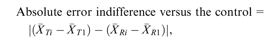
\begin{matrix} Absolute error indifference versus the control = \\ | ({\bar{X}}_{Ti} - {\bar{X}}_{T 1}) - ({\bar{X}}_{Ri} - {\bar{X}}_{R 1}) |, \end{matrix}

where i represents each treatment being investigated and 1 represents the no-treatment arm. This was estimated for each treatment separately.

Sensitivity Analyses

One of the important assumptions when using external data for only one of the treatment arms is what happens to the treatment effect after follow-up. Although a rationale was given in the methods and a distribution was used to account for a degree of uncertainty, the time it takes for a hazard ratio to taper to 1 may be difficult to estimate statistically and/or for medical experts to give an opinion on. For systemic treatments, where patients may not be expected to receive the treatment under investigation long after follow-up, such as those in the data used by Guyot et al.,¹⁵ medical experts may be able to give a reasonable estimate for how long they expect the treatment effect to last. However, because the data used in this study contained nonsystemic interventions that may have long-lasting effects or even curative effects, there is greater uncertainty over the treatment effect after follow-up.

For this study, 2 approaches using statistical methods were considered to estimate the time for the hazard ratio to equal 1. The first method involved plotting the predicted extrapolated hazard ratios from an ensemble of parametric models and from stratified flexible spline–based models with 3 knots for each follow-up time and the complete data set. The second involved the use of the Bayesian simultaneous model, with priors indicating a negligible treatment effect after follow-up, specifically, normal priors for the hazard ratios with a mean of 1 and precision of 100 within each year after follow-up. The first method proved useful for the radiotherapy arm, which crossed the hazard ratio of 1 line at 12 months, but it gave little insight for the radiotherapy arm, and even models fitted to the complete data set showed little or no evidence of hazard ratio tapering for the radiotherapy arm. However, the Bayesian approach did give reasonably consistent and plausible estimates across all follow-up times studied for the radiotherapy arm, and these results are presented. The sensitivity analyses are presented in the appendix.

Statistical Software

Kaplan-Meier charts were digitized using Plot Digitizer.³³ Frequentist survival analyses were conducted in R³⁴ using the eha package³⁵ and flexsurv package.³⁶ Smoothed hazard rates were estimated using the survPresmooth package.³⁷ Area under the survival curves was estimated using the MESS package.³⁸ Charts were produced using the ggplot2 package.³⁹ Bayesian analyses were conducted using JAGS.⁴⁰ The WAIC values were estimated using the loo package.³² Code is presented in the appendix for some of the methods, which includes the Bayesian and hybrid models.

Role of Funding

The study had no external funding source.

Results

The results of the evaluation statistics are presented for 1 to 10 years of follow-up. Example survival curves and predicted mean overall survival distributions are presented for a 4-year follow-up. This time point was chosen because it gave enough data to see whether a model could fit the short-term data but left a large proportion of the curve still unknown.

Example Results with 4 Years of Follow-up

Five of the parametric models (exponential, Weibull, stratified Weibull, generalized gamma, and Royston and Parmar²⁴ 1-knot spline model assuming proportional hazards) were able to give reasonable predictions when there was a small short-term benefit (radiotherapy) or small long-term benefit (radiotherapy plus surgery). However, none of the parametric models were able to produce plausible predictions when there was a large long-term benefit (surgery), given that the minimum age of patients in the Ganti et al.¹⁸ study was 80 years. The exponential model came closest to producing plausible estimates for all 10 follow-up times and was therefore selected from among the parametric models. The online appendix presents model predictions for the data cut at 4 years (Suppl. Figures S8–S9) as well as AIC and BIC fit statistics (Suppl. Figure S10).

The hybrid models also had difficulty producing plausible predictions, with the exponential model getting closest to giving plausible predictions for all treatments across the 10 follow-up times. The hybrid exponential model was able to give reasonable predictions when there was a small short-term benefit (radiotherapy) or small long-term benefit (radiotherapy plus surgery) but did not give plausible predictions when there was a large long-term benefit (surgery). Supplemental Figure S11 in the online appendix presents model predictions for the data cut at 4 years and Supplemental Table S1 in the appendix presents the probability of best-fitting model.

Using the predicted hazard rates from the external data and applying hazard ratio tapering forced all the models to give plausible predictions (Suppl. Figures S12–S14 in the online appendix).

Suppl. Figure S15 presents the survival predictions from the 6 methods tested for the 4-year data set. Applying the external data and hazard ratio tapering to the most plausible parametric model (exponential) and most plausible hybrid model (exponential) resulted in survival curves that appeared to fit all the treatment arms well and gave plausible predictions for each treatment arm. The ensemble of parametric models with external data extrapolation also gave a good visual fit to the data and included greater uncertainly as it was able to capture the error for the choice of model. The Bayesian simultaneous model gave a reasonable fit to the data for the scenarios where there was a small benefit but underestimated survival for the scenario with a large long-term benefit.

Supplemental Figure S16 presents the distributions for predicted mean overall survival for the 6 methods, together with the distributions estimated from the reference model fitted to the complete data set. All models were able to give reasonable predictions for the scenario with a small short-term benefit (radiotherapy). For the scenario for a small long-term benefit, the 2 models that did not use external data (simple exponential model and hybrid exponential model) underestimated survival; the other models all gave predictions that matched closely those from the complete data set. For the scenario for a large long-term benefit, the 2 models that did not use external data (simple exponential model and hybrid exponential model) overestimated survival, whereas the models that modeled the external data separately gave a close fit to the predictions from the complete data. The Bayesian simultaneous model appeared to underestimate survival for this scenario.

Results from the Model Evaluation Statistics

Figure 3 (color version is provided in the online appendix) presents the results from the evaluation statistics for each of the 6 models investigated, for each of the 10 follow-up times, and by the 3 treatment scenarios. No single model performed well across all 3 scenarios.

Figure 3

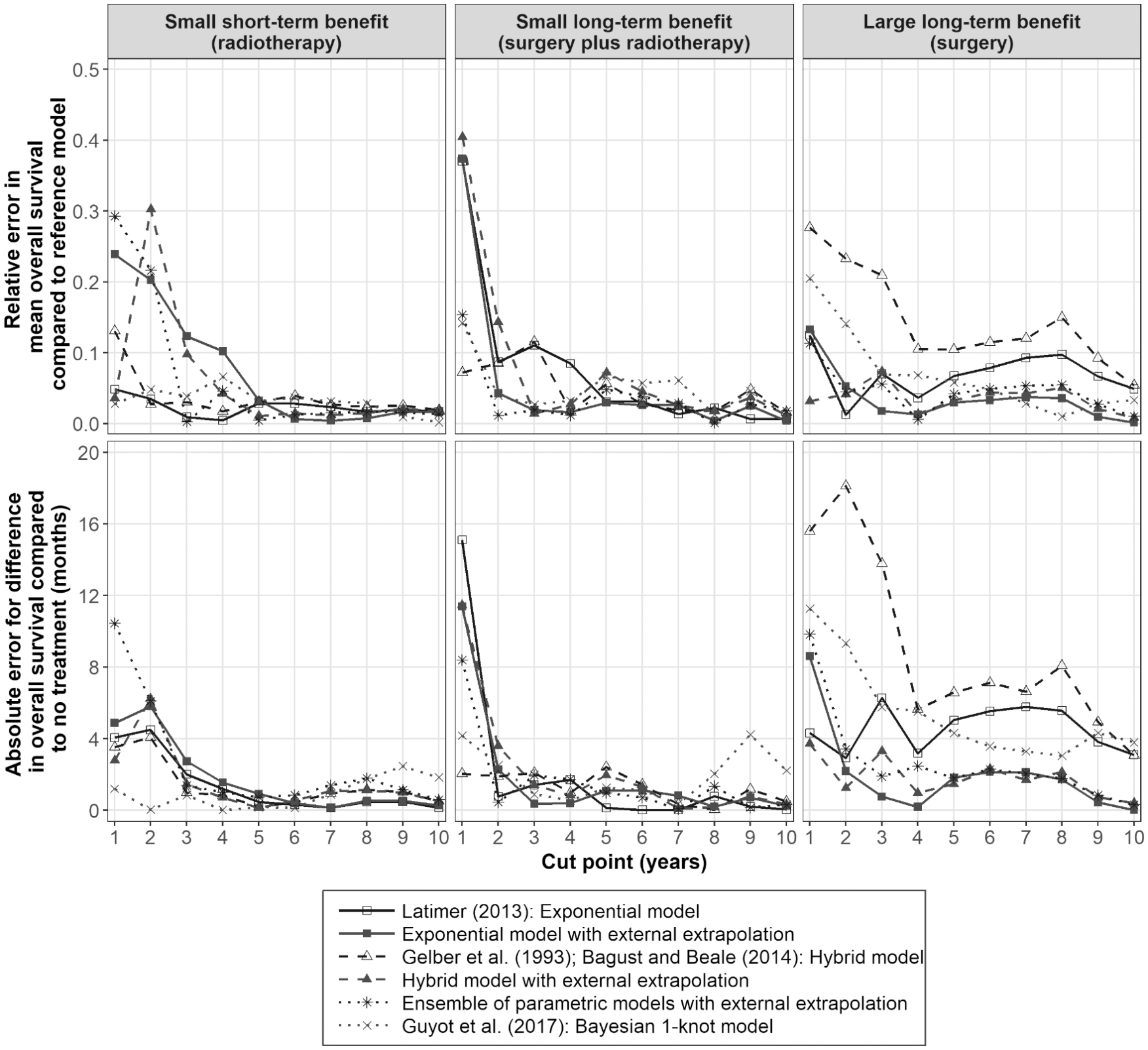
Model evaluation for predicted distributions for mean survival compared to the model fitted to the complete data set and for predicted distributions for the difference in mean survival v. no treatment compared to the model fitted to the complete data set. Relative error is the difference in predicted mean overall survival v. that estimated from the complete data divided by the mean overall survival time estimated from the complete data set; absolute error is the difference in predicted mean overall survival v. that estimated from the complete data.

For the scenario for a small short-term benefit (radiotherapy), the Guyot et al.¹⁵ model performed particularly well, even with a short follow-up time (≤3 years) for all the evaluation statistics. The models using the external data with hazard ratio tapering performed less well compared with the other models until a follow-up of 5 years had been reached. This result may reflect the assumption that the long-term hazard ratio tapering effect is the same for all treatments. The hazard rates for radiotherapy were greater than or equal to those estimated for the no-treatment arm from 1 to 7 years (Suppl. Figure S2). If the information from these smooth hazard plots had been used and had the hazard ratio tapering assumption been adjusted to no-treatment effect after follow-up, it is likely these models would have performed better. However, these results suggest that, unlike the other models that use external data, the Guyot et al.¹⁵ model may be reasonably robust in detecting when there is a small, short-term treatment effect in the data, but a long-term treatment effect is assumed when fitting the model.

For the scenario for a small long-term benefit (surgery plus radiotherapy), where the proportional hazard assumption approximately holds, all models performed well with follow-up times of ≥2 years.

For the scenario of a large long-term benefit (surgery), the methods that used long-term external data separately performed better than the other models. The hybrid model without external data extrapolation performed the worst across all follow-up times, followed by the method described by Latimer⁴ and the Guyot et al.¹⁵ model. The models that used external data with hazard ratio tapering were able to give reliable predictions with follow-up times of ≥2 years.

When less informative priors for the hazard ratio tapering (prior standard deviation of 4 for the hazard ratio) were used as sensitivity analyses in the Guyot et al.¹⁵ model, the model performed better in the scenario with a large long-term benefit (surgery) and less well in the scenario with a small long-term benefit (surgery plus radiotherapy) arm. These results are therefore difficult to generalize to other studies and were likely due to the 1-spline knot being insufficient to describe the shape of the hazard trajectory in each treatment group; convergence could not be achieved with more complex models.

Further investigations were conducted for the hazard ratio tapering assumptions used in the ensemble method and the Guyot et al.¹⁵ model. Predicted hazard ratios from these 2 methods for the 4-year data set and those from parametric models fitted to the complete data are presented in the online appendix (Suppl. Figure S17). There was little or no indication of hazard ratios tapering to 1 for the radiotherapy plus surgery and surgery arms from models fitted to the complete data set, despite both models needing hazard ratios to taper to 1 before 20 years to give biologically plausible predictions for the surgery data. Figure 4 (color version presented in online appendix) presents the hazard ratios from the Bayesian simultaneous model for the 4-year follow-up data and the predicted time at which the hazard ratio tapered to 1 for all 10 data sets. Sensitivity analyses for the time for the hazard ratio to reach 1 (no treatment effect after follow-up and hazard ratio tapers to 1 at 20 years) are presented in the online appendix (Suppl. Figure S18). These results show that the correct value is between 4 and 20 years. Changing the time for the hazard ratio to taper to 1 from 10 to 13.5 years with a standard deviation of 1.4 (Suppl. Figure S19 in the online appendix) improved the predictions from the Guyot et al.¹⁵ model, but it had little impact on those from the method based on the ensemble methods, suggesting the models that used the external data separately may be reasonably robust to the assumption regarding the treatment effect after follow-up. This outcome is likely because the time to the hazard ratio tapering to 1 for the models that used the external data separately was assumed to be based on a relatively broad distribution. For this study, making the prior less informative with the Bayesian model did not alleviate the problem, as this produced biologically implausible predictions in the surgery arm and fitted the data less well in the surgery plus radiotherapy arm. This problem was likely due to the Bayesian model being too simple to model all the treatment arms. This may not be the case for other data sets.

Figure 4

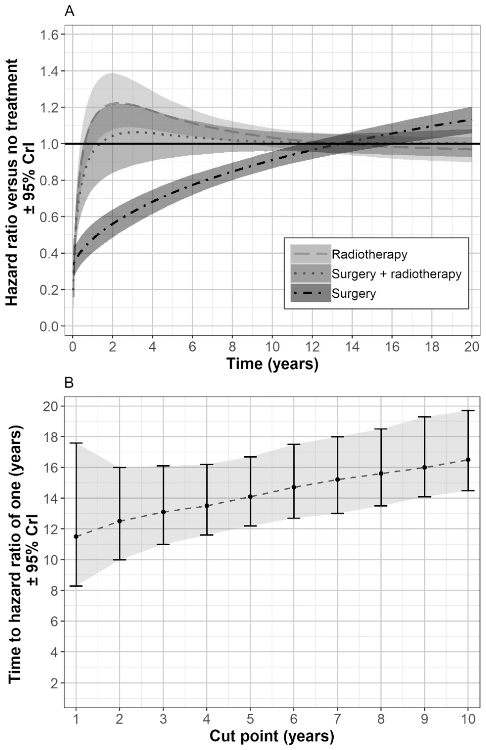
The Guyot et al.¹⁵ model used to predict the time at which the hazard ratios taper to 1. Predicted hazard ratio, from the data cut at 4 years and priors for no treatment effect after follow-up (A). Predicted time to a hazard ratio of 1 for surgery from Bayesian models fitted to each of the 10 data sets, with priors for no treatment effect after follow-up (B). CrI, credible interval.

Discussion

The results from this study suggest that when the treatment benefit is small (hazard ratio = 1 ±≤0.3), survival curve extrapolation, without the use of external data, may be reasonably accurate. If the survival at end of follow-up is ≤30%, then the Guyot et al.¹⁵ model is likely to produce the most accurate predictions and appeared in this study to be robust to overestimating the time at which the hazard ratio equals 1. Under the Guyot et al.¹⁵ model, while the prior mean tapers linearly through time, the model allows for uncertainty about the exact value of the hazard ratio at each time, by allowing the hazard ratio at each time to vary independently around the corresponding prior mean. Therefore, the Guyot et al.¹⁵ model is robust to different assumptions about the short-term treatment effect. The other methods that used external data performed less well when the duration of treatment effect was small, which may have been due to overestimating the time for the hazard ratio to equal 1.

When the treatment benefit was large (in this study, the hazard ratio was 0.37 for surgery) and treatment effect covered a long duration, utilization of external data with hazard ratio tapering was needed to produce accurate long-term predictions. Simple parametric models with hazard ratio tapering may be sufficient if they fit the data well and produce plausible long-term predictions. For other data sets, more complex models may be needed, such as the hybrid model with hazard ratio tapering or the ensemble approach with hazard ratio tapering. The Guyot et al.¹⁵ model performed less well for the scenario with a large, long-term treatment effect. This may have been due to this model being too simple to fit all treatment arms well in this study and being sensitive to the priors used for the hazard ratio tapering effect and the assumed time to when hazard ratios equal 1. For the other models that used external data, a broad distribution was assumed for the time to hazard ratio equaling 1, which made them more robust to the uncertainty of when the hazard ratio converged to 1.

It is likely that when clinical advice suggests the duration of treatment effect is short, the Guyot et al.¹⁵ model may be reasonably accurate so long as the model fits all study arms well, but when the duration of treatment effect is believed to be long or unknown, separate modeling of the hazard ratio over time may be required, which can capture a greater uncertainty. Where the treatment benefit is expected to be large and the probability of an event at end of follow-up has not reached 30%, then estimates of mean overall survival from all models are likely to be unreliable.

This study has shown that covariate data may not be needed to match external data to trial data, as a time acceleration adjustment may be sufficient. Matching external data to RCT data may be problematic, as long-term external data are likely to include patients who entered the study at a longer time in the past compared to those in the trial. Improvements in standard of care over time are likely to be considerable in oncology and other disease areas. If there is more than 1 source of external data, sensitivity analyses could be conducted, or a meta-survival model could be used such as that described by Vickers et al.⁴¹

The data used in this study were from elderly patients (≥80 years old), in whom general age-related mortality was a factor, which was not detectable in the short-term data. This resulted in methods that did not use long-term external data and general population data producing biased predictions. For this study, the extrapolation of parametric models described by Latimer⁴ and the hybrid models described by Gelber et al.¹⁰ and Bagust and Beale,¹¹ which did not use external data, were not able to provide accurate long-term predictions. This poor accuracy was likely due to these models not accounting for a change in hazard rates after follow-up and due to the hybrid model giving large prediction errors because the parametric model was fitted only to a reduced sample of patients. It would be interesting to see how these models perform in younger patient populations.

Another limitation of this study was its reliance on observational data. Differences in outcome were attributed to treatment for the purposes of this study. However, treatment effect and the duration of treatment effect after follow-up could have been due, at least in part, to the criteria used to assess how suitable patients were to receive radiotherapy and/or surgery. However, this issue is less relevant if the survival curve data used in this study are representative of data from RCTs.

The utilization of external data and application of hazard ratio tapering does have limitations. The most important of which is likely to be the assumption regarding what happens to the treatment effect after follow-up. Grieve et al.⁶ argue that the time taken for the hazard ratio to equal 1 could be estimated by modeling the time-varying treatment effects from the RCT data. However, Jackson et al.¹⁶ argue that long-term assumptions, such as proportional hazards, are untestable from data. From the data used in the current study, only the hazard ratios for radiotherapy alone crossed the hazard ratio equal to 1 line in a short time (1 year). For the other treatments, even with the complete data, there was little evidence of what happens to hazard ratios after follow-up because survival in the surgery arm was much longer than that in the no-treatment arm, and the models fitted to the complete data with time-varying effects showed little evidence of the hazard rates converging. However, this study has provided evidence that a Bayesian approach with priors for no treatment effect after follow-up may help support the choice of what to assume after follow-up, although it is sensitive to the precision used for the priors. If this method had been followed separately for each timepoint and for each treatment, it is likely that model performance would have been improved for the models using external data for the scenarios tested where there was only a short-term treatment effect. Sensitivity analyses are still required to investigate the assumption of what happens to the treatment effect after the end of follow-up. Jackson et al.¹⁶ provide a thorough review of other difficulties in survival curve extrapolation and the assumptions needed.

If the current study is representative of oncology trial data, extrapolating survival curves remains challenging, especially when the treatment effect is large and the probability of no event is >70% at the end of follow-up. This study suggests that under these circumstances, there is a risk of stating mean survival estimates and differences in mean survival that are statistically different from what might be observed with mature data. The results from this study support the argument that direct use of long-term data is needed to make long-term predictions, regardless of the extent to which the survival curves are complete. In particular, the Guyot et al.¹⁵ study appeared to be most suitable when the treatment effect was small (hazard ratio in this study was 0.70) and the separate use of external data appeared to be most appropriate when the treatment effect was large (hazard ratio in this study was 0.37).

Supplemental Material

Online_appendix_11_October_2019_online_supp – Supplemental material for An Evaluation of Survival Curve Extrapolation Techniques Using Long-Term Observational Cancer Data

Supplemental material, Online_appendix_11_October_2019_online_supp for An Evaluation of Survival Curve Extrapolation Techniques Using Long-Term Observational Cancer Data by Adrian Vickers in Medical Decision Making

Supplemental Material

R_and_JAGS_code_31_July_2019_online_supp – Supplemental material for An Evaluation of Survival Curve Extrapolation Techniques Using Long-Term Observational Cancer Data

Supplemental material, R_and_JAGS_code_31_July_2019_online_supp for An Evaluation of Survival Curve Extrapolation Techniques Using Long-Term Observational Cancer Data by Adrian Vickers in Medical Decision Making

Footnotes

Acknowledgements

The author is grateful to comments from Stephen Kay at Model Outcomes Limited, from colleagues at RTI Health Solutions, and 3 anonymous reviewers whose comments led to a substantially improved manuscript.

The author(s) declared no potential conflicts of interest with respect to the research, authorship, and/or publication of this article.

The author(s) received no financial support for the research, authorship, and/or publication of this article.

ORCID iD

Adrian Vickers

Supplemental Material

Supplementary material for this article is available on the Medical Decision Making Web site at .

References

Conn

Johnson

Boveng

PL.

On extrapolating past the range of observed data when making statistical predictions in ecology. PLoS One. 2015;10(10):e0141416.

Latimer

NR.

Survival analysis for economic evaluations alongside clinical trials—extrapolation with patient-level data: inconsistencies, limitations, and a practical guide. Med Decis Making. 2013;33:743–54.

Davies

Briggs

Lorgelly

Garellick

Malchau

The “hazards” of extrapolating survival curves. Med Decis Making. 2013;33:369–80.

Latimer

NICE DSU Technical Support Document 14: Undertaking survival analysis for economic evaluations alongside clinical trials—extrapolation with patient-level data. 2013. Available from: http://www.nicedsu.org.uk

NICE. Guide to the methods of technology appraisal, third edition draft for consultation. 2013. Available from: URL: http://publications.nice.org.uk/guide-to-the-methods-of-technology-appraisal2013-pmg9/the-reference-case

Grieve

Hawkins

Pennington

Extrapolation of survival data in cost-effectiveness analysis: improving the current state of play. Med Decis Making. 2013;33(6):740–2.

Negrin

Nam

Briggs

AH.

Bayesian solutions for handling uncertainty in survival extrapolation. Med Decis Making. 2017;37(4):367–76.

Annest

Bumgarner

Raftery

Yeung

KY.

Iterative Bayesian model averaging: a method for the application of survival analysis to high-dimensional microarray data. BMC Bioinformatics. 2009;10:72.

Raftery

Painter

Volinsky

CT.

BMA: an R package for Bayesian model averaging. R News. 2005;5(2):2–8.

10.

Gelber

Goldhirsch

Cole

BF.

Parametric extrapolation of survival estimates with applications to quality of life evaluation of treatments. Control Clin Trials. 1993;14:485–99.

11.

Bagust

Beale

Survival analysis and extrapolation modeling of time-to-event clinical trial data for economic evaluation: an alternative approach. Med Decis Making. 2014;34(3):343–51.

12.

Bengalia

Jackson

Sharples

LD.

Survival extrapolation in the presence of cause specific hazards. Stat Med. 2015;34:796–811.

13.

Demiris

Lunn

Sharples

LD.

Survival extrapolation using the poly-Weibull model. Stat Methods Med Res. 2015;24(2):287–301.

14.

Lambert

PC.

Modeling of the cure fraction in survival studies. Stata J. 2007;7(3):1–25.

15.

Guyot

Ades

Beasley

Lueza

Pignon

J-P

Welton

NJ.

Extrapolation of trial-based survival curves using external information. Med Decis Making. 2017;37(4):353–66.

16.

Jackson

Stevens

Ren

, et al. Extrapolating survival from randomized trials using external data: a review of methods. Med Decis Making. 2017; 37(4):377–90.

17.

Kim

Thompson

SG.

Uncertainty and validation of health economic decision models. Health Econ. 2010;19:43–55.

18.

Ganti

Shostrom

Alorabi

, et al. Early stage non-small-cell lung cancer in octogenarian and older patients: a SEER database analysis. Clin Lung Cancer. 2016;17(4):285–91.

19.

Guyot

Ades

Ouwens

Welton

NJ.

Enhanced secondary analysis of survival data: reconstructing the data from published Kaplan-Meier survival curves. BMC Med Res Methodol. 2012;12(9):1–13.

20.

Bach

Laura

Cramer

Warren

Begg

CB.

Racial differences in the treatment of early stage cancer. N Engl J Med. 1999;341(16):1198–205.

21.

Clark

Bradburn

Love

Altman

DG.

Survival analysis part I: basic concepts and first analyses. Br J Cancer. 2003;89:232–38.

22.

Bell

Miller

ML.

Life tables for the United States Social Security Area 1900–2100. Actual Study No. 120. 2005 August. Available from:https://www.ssa.gov/oact/NOTES/as120/LifeTables_Tbl_6_2010.html

23.

Howden

Meyer

. Age and sex composition: 2010. 2010 Census Briefs. United States Census Bureau. Available at http://www.census.gov/prod/cen2010/briefs/c2010br-03.pdf. Accessed 9 April 2018.

24.

Royston

Parmar

Flexible parametric proportional-hazards and proportional-odds models for censored survival data, with application to prognostic modelling and estimation of treatment effects. Stat Med. 2002;21(1):2175–97.

25.

Efron

Censored data and the bootstrap. J Am Stat Assoc. 1981;76(374):312–19.

26.

Chow

GC.

Tests of equality between sets of coefficients in two linear regressions. Econometrica. 1960;28(3):591–605.

27.

Buckland

Burnham

Augustin

NH.

Model selection: an integral part of inference. Biometrics. 1997;53:606–18.

28.

Burnham

Anderson

DR.

Model Selection and Multimodel Inference. A Practical Information-Theoretic Approach. 2nd ed. New York, NY: Springer-Verlag; 2002.

29.

Jackson

Thompson

Sharples

LD.

Accounting for uncertainty in health economic decision models by using model averaging. J R Statist Soc A. 2009;172(2):383–404.

30.

Jackson

Bojke

Thompson

Claxton

Sharples

LD.

A framework for addressing structural uncertainty in decision models. Med Decis Making. 2011;31(4):662–74.

31.

Herring

Pearson

Purser

, et al. Cost effectiveness of ofatumumab plus chlorambucil in first-line chronic lymphocytic leukaemia in Canada. Pharmacoeconomics. 2016;34:77–90.

32.

Vehtari

Gelman

Gabry

Practical Bayesian model evaluation using leave-one-out cross-validation and WAIC. Statis Comput. 2017;27(5):1413–32.

33.

Huwaldt

Stienhorst

Plot Digitizer. Version 2.6.8. 2015. Available from: http://plotdigitizer.sourceforge.net

34.

R Development Core Team. R Version 3.4.3: A Language and Environment for Statistical Computing. Vienna, Austria: R Foundation for Statistical Computing; 2017.

35.

Brostron

Event History Analysis with R. Boca Raton, FL: CRC Press; 2012.

36.

Jackson

CH.

flexsurv: A platform for parametric survival modeling in R. J Stat Softw. 2016;70(8):1–33.

37.

Lopez-de-Ullibarri

Jacome

MA.

survPresmooth: an R package for presmoothed estimation in survival analysis. J Stat Softw. 2013;54(11):1–26.

38.

Ekstrom

CT.

The R Primer. 2nd ed.2016. Boca Raton, FL: Chapman & Hall, CRC Press; 2016.

39.

Wickham

ggplot2 Elegant Graphics for Data Analysis. New York, NY: Springer; 2009.

40.

Plummer

JAGS: a program for analysis of Bayesian graphical models using Gibbs sampling. Proceedings of the Third International Workshop on Distributed Statistical Computing; Vienna, Austria. March 20–22, 2003. Available from: http://www.r-project.org/conferences/DSC-2003/Proceedings/Plummer.pdf

41.

Vickers

Winfree

Cuyen Carter

, et al. Relative efficacy of interventions in the treatment of second-line non-small cell lung cancer: a systematic review and network meta-analysis. BMC Cancer. 2019;19(1):353.

Supplementary Material

Please find the following supplemental material available below.

For Open Access articles published under a Creative Commons License, all supplemental material carries the same license as the article it is associated with.

For non-Open Access articles published, all supplemental material carries a non-exclusive license, and permission requests for re-use of supplemental material or any part of supplemental material shall be sent directly to the copyright owner as specified in the copyright notice associated with the article.

0.00 MB

1.31 MB

0.01 MB