
Abstract
Keywords
Cost-effectiveness analyses (CEAs) that use data from well-designed randomized studies can provide a sound basis for policy making if they use suitable methods. 1 Statistical methods have been developed that accommodate the hierarchical structure of cost and health outcome data from multicenter randomized controlled trials2–4 or cluster randomized trials (CRTs).5,6 A general methodological concern is that there may be missing resource use or outcome data—for example, because patients are lost to follow-up or they do not return or complete quality-of-life (QoL) or resource use questionnaires. Multiple imputation (MI) has been proposed for handling missing data in CEAs.7–11 However, the approaches proposed may not be appropriate for CEAs that use data from multicenter or cluster trials, because they fail to recognize that data may be clustered within settings. If missing data are not addressed appropriately, this can lead to misleading results. 12
The approach taken to handling missing data should aim to provide unbiased, efficient estimates. This requires reasons for missing costs or health outcomes to be carefully considered. However, most published CEAs simply discard the observations with missing data and report complete case analyses (CCAs). 13 This unprincipled approach assumes that the data are missing completely at random (MCAR); that is, missing values do not depend on any observed or unobserved variable. 14 If observations with missing endpoints differ from those with complete information, CCA will lead to inaccurate cost-effectiveness estimates. 8 Principled approaches for handling missing data, such as MI, maximum likelihood estimation, and full-Bayesian analyses, assume that data are missing at random (MAR). 14 That is, the probability of missing data is independent of any unobserved variable given the observed data. If the probability of missing data is associated with unobserved values, then the data are termed missing not at random (MNAR). 14
MI is an attractive method for addressing missing data in CEAs when values are MAR. A distinct feature of MI is that the model for the missing values is specified separately from the analytical model for estimating the parameters of interest. In the imputation model we can incorporate information contained in observed variables that are associated both with the outcome and with the probability that data are missing. If these variables are beyond those included in the analysis model, for example, postrandomization variables such as length of hospital stay, they are called auxiliary variables. Including such auxiliary variables in the imputation model can reduce bias, can improve efficiency, and may make the MAR assumption more plausible than maximum likelihood approaches.
For MI to provide valid inferences, the imputation model must appropriately recognize the structure of the data. In CRTs, randomization is at the level of the cluster (e.g., the primary care provider), not the individual. In CEAs that use CRTs, the probability of missing costs or health outcomes may be more similar within than across clusters.15–17 For example, missingness may depend on individual-level characteristics, which tend to be more similar within the cluster, and on cluster-level characteristics, such as whether the cluster is a teaching hospital. However, previous CEAs based on CRTs have not used imputation models that accommodate clustering. We found that of 62 studies included in a previous systematic review, 18 38 reported missing data, which in 35 studies was addressed with unprincipled methods (27 used CCA, 6 mean imputation, 2 last observation carried forward). The other 3 studies adopted single-level MI, whereby the imputation model ignored any clustering. When the probability of missingness has a multilevel structure, single-level MI can lead to biased point estimates and incorrect uncertainty measures. 12 Instead, multilevel MI recognizes that the data may be hierarchical12,19 and has recently been proposed for CEAs that use CRTs. 20 There is no previous evidence on the relative performance of multilevel MI versus single-level MI or CCA for CEAs that use CRTs.
This paper aims to compare a multilevel MI approach with single-level MI and CCA in CEAs that use CRTs. We extend previous work 20 by considering the performance of methods across a wide range of circumstances faced by CEAs that use CRTs. We generate different scenarios with missing data from a fully observed data set, 12 in this case a previous CEA. 21 Informed by the methodological literature,10,11,15,17 we consider alternative settings that differ according to the missing data mechanisms (MCAR, MAR, MNAR), the proportion of observations with missing endpoint data (10%, 30%, 50%), the type of covariate that explains missingness (binary or continuous, patient-level, or cluster-level), and the endpoint assumed to be missing (cost, outcome, or both cost and outcome).
In the next section, we outline alternative MI methods for CEAs that use CRTs. Next we introduce the case study, the framework for generating the missing data, and the scenarios considered. We then report the results from applying the alternative methods to the missing data scenarios, discuss the findings, and outline an agenda for further research.
Methods
Important methodological considerations must be recognized by the approach to handling missing data in CEAs. First, the approach to handling the missing data needs to recognize that the reasons for missing data may differ by treatment group and endpoint. Second, the probability of missingness for one endpoint (e.g., cost) may depend on the level of another endpoint (e.g., utility). Third, the missing data approach should recognize that endpoints and covariates may have nonnormal distributions.8,11 Fourth, the approach to handling the missing data should appropriately recognize the data structure and be compatible with the model for the endpoints.12,16 For example, in CEAs that use CRTs, methods for handling missing data should accommodate the hierarchical structure of the data. 20
Multiple Imputation
In MI, the key idea is to replace each missing value with a set of M plausible values. 22 Each of these values is drawn, in a Bayesian manner, from the conditional distribution of the missing observations given the observed data, so that the set of imputed values reflects the uncertainty associated with both the missing data and the estimation of the parameters in the imputation model. This is repeated M times, and in each imputation data set each missing observation is replaced with an imputed value from the set of imputed values. The analysis model, for example, a multilevel model, is then applied to each completed data set to estimate the parameters of interest. These M sets of estimates and accompanying measures of uncertainty are then combined using Rubin's rules 22 to properly reflect the variation both within and between imputations.
We consider 2 MI approaches, single-level MI
22
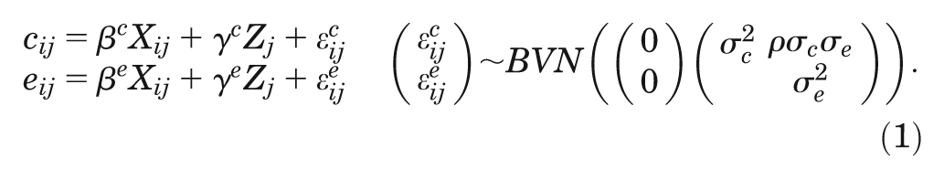
and multilevel MI.12,19 We use the following notation: Let cij and
eij represent the costs and outcomes for the ith
individual within the jth cluster, and let
Model 1: single-level MI
A single-level imputation model for costs and health outcomes
Model 1 is applied separately by treatment groups (for tj = 0 and
tj = 1) to recognize that the posterior conditional distribution of the
missing data given the observed may differ across treatment arms.
23
An alternative is to include in Model 1 a treatment
indicator as a covariate, but this assumes that the variances
M imputations are then generated as follows 22 :
Draw values for
Generate imputed values for each missing observation (
Repeat steps 1 and 2, M times.
Single-level MI may account for some of the clustering if cluster-level covariates (e.g., whether the cluster is a teaching hospital or not) that help explain between-cluster variability are included in the imputation model as auxiliary variables. However, it is unlikely that this approach will account for all the between-cluster heterogeneity. The imputed values are drawn from the conditional distribution of the missing observations given the observed data, ignoring any dependency between observations within a cluster not explained by the auxiliary variables included in the model. Therefore, the single-level imputation model does not properly represent the conditional distribution of the missing data given the observed data and can lead to invalid inferences. 12
Model 2: multilevel MI
Multilevel MI explicitly recognizes the clustering by extending Model 1 to incorporate
cluster-specific random effects,
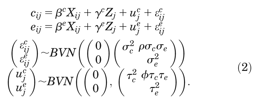
The random effects are assumed to follow a BVN distribution with variances
A multilevel MI approach for generating the M imputations can be described as follows19,24:
Sample
Draw values for
Generate imputed values for
Repeat steps 1–3, M times.
Both MI approaches assume that the imputed values are drawn from a BVN. However, because costs
are typically right skewed, it is recommended that before imputation, a transformation (e.g., log)
is taken to help make the normality assumption more plausible.8,11,25 The transformed costs
are then multiply imputed and back-transformed onto the original scale before applying the analysis
model. For both approaches, uniform priors are usually assumed for the fixed-effects regression
coefficients (
Overview of the Case Study
We used cost-effectiveness data from a CRT that evaluated an intervention to improve diagnosis of
active labor in primiparous women.
26
The intervention consisted of a decision support algorithm to help midwives
diagnose active labor, which was compared with standard care (control group). The CEA was typical of
a study based on a CRT,
18
in
that few clusters were randomized (14 maternity units in Scotland, 2171 patients), there were
unequal numbers of individuals per cluster (49–198), intracluster correlation coefficients (ICCs)
were low for the outcome measure (ICC ≈ 0.03) but relatively high for costs (ICC ≈ 0.14),* and individual costs and outcomes were correlated
(
The primary CEA took as the effectiveness endpoint a measure of process utility 21 because, unlike measures of QoL or clinical outcome, it was anticipated to be sensitive to any effect that the intervention may have on the care process. 28 The measure encompassed women's preferences for those aspects of the labor experience that were deemed important to women and expected to differ between treatment arms. 28 These included number of hospital visits before labor ward admission, length of stay on the labor ward, mobility during labor, pain relief required, and mode of delivery. Information on the process of care according to each attribute was collected from the case records of the women enrolled in the CRT. A discrete choice experiment (DCE) was undertaken on a representative sample of women included in the CRT to elicit their preferences for each attribute. The actual experience of each woman was then valued according to the preferences elicited from the DCE, to report an overall measure of process utility. 21 This measure of process utility was expressed in terms of women's willingness to trade between each attribute and time spent on the labor ward (marginal disutility of increasing time in the labor ward), providing an overall estimate of willingness to wait (WTW), 28 where higher WTW means “better” process utility. Health service costs per patient (£ sterling, 2005–2006) were calculated by recording information on resource use on the labor ward before and after birth and then combining these resource use measures with standard unit costs for obstetric admissions. 21 In the CRT, information was collected on individual- and cluster-level covariates anticipated to be associated with cost and WTW.
In Table 1, we report summary statistics for the cost and process utility (WTW) endpoints and for individual- and cluster-level covariates. Each covariate had a moderate association with costs and a strong association with WTW (Table 2). The association of cluster size with either endpoint appeared to differ by randomized arm. The size of the randomized cluster also differed across treatment arms (Table 2, last column); the average number of women randomized in each cluster was higher for the control group.
Descriptive Statistics for the Fully Observed Data in the Case Study
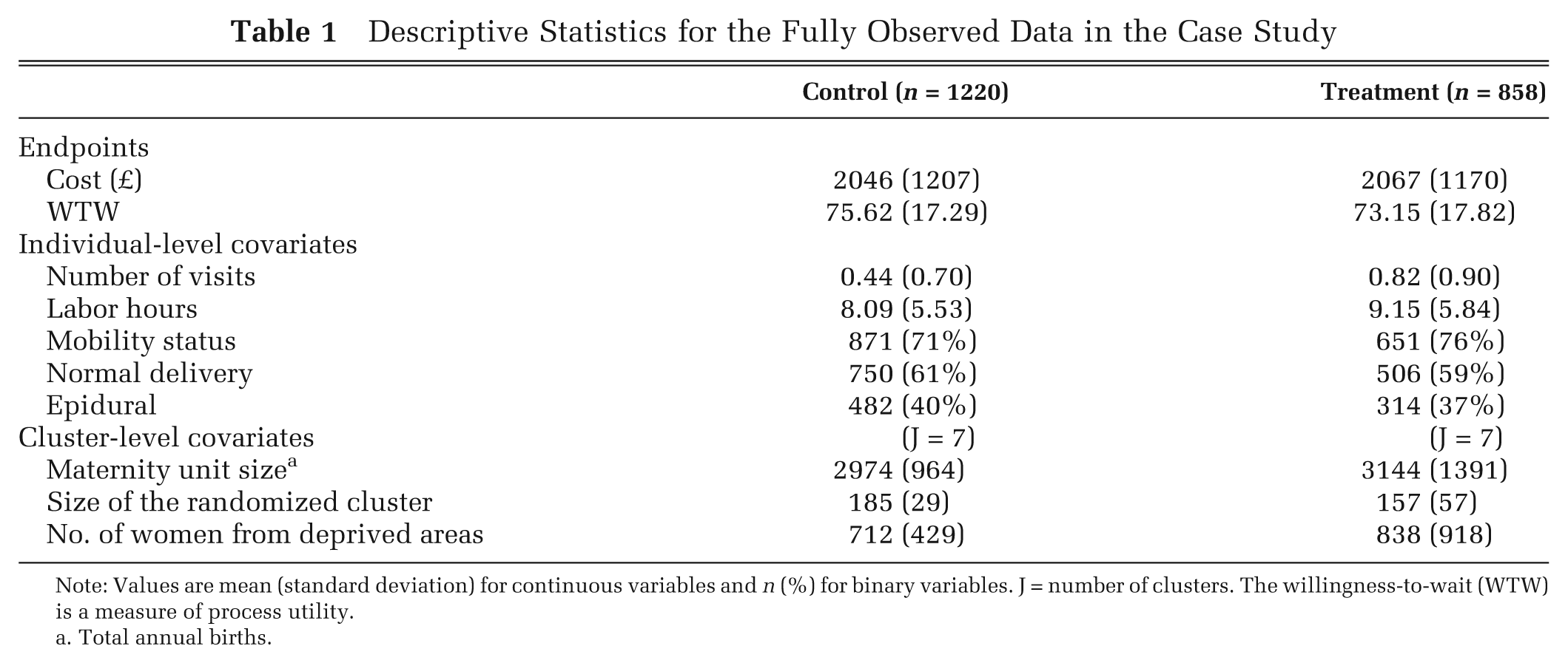
Note: Values are mean (standard deviation) for continuous variables and n (%) for binary variables. J = number of clusters. The willingness-to-wait (WTW) is a measure of process utility.
Total annual births.
Correlation of Each Covariate with Cost and WTW Endpoints by Treatment Arm, and Standardized Mean Difference of Each Covariate between Treatment Groups
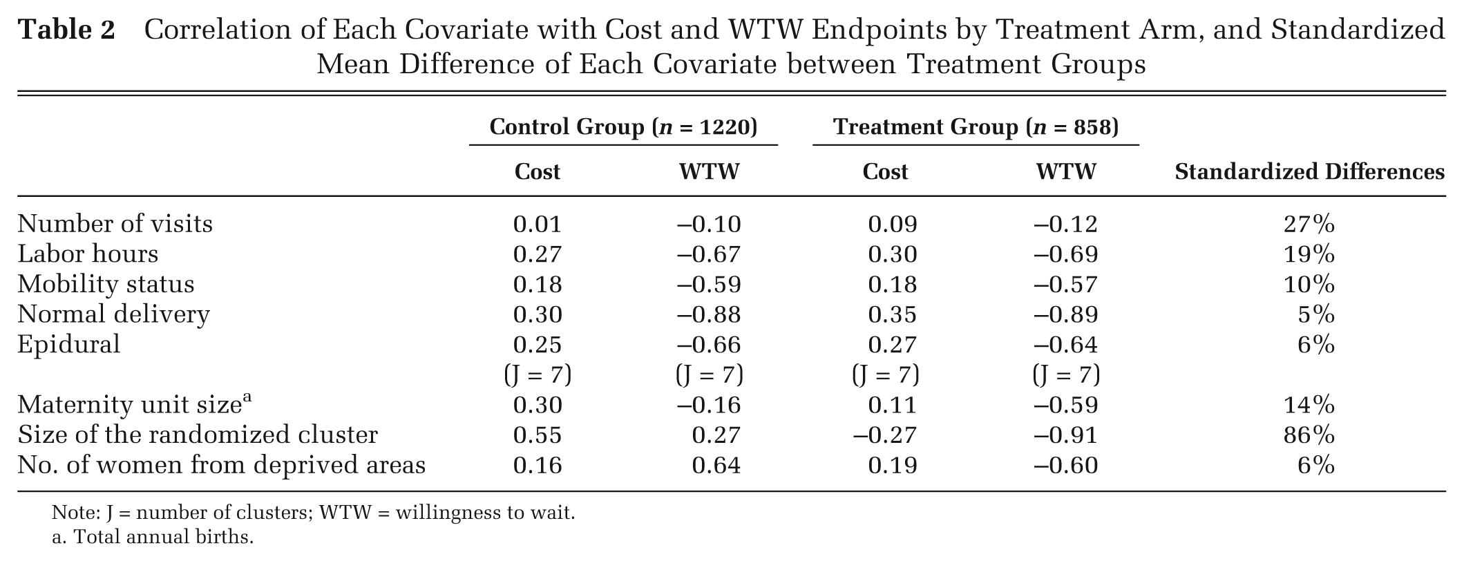
Note: J = number of clusters; WTW = willingness to wait.
Total annual births.
We took the cost-effectiveness threshold (λ) as the mean willingness to pay (WTP) per hour reduction in the time on the labor ward. The value for λ that we used in the base case (£32) was taken from a previous DCE. 29 We reported cost-effectiveness according to incremental net monetary benefit (INB), by valuing the incremental WTW for treatment versus control by λ and subtracting from this the incremental cost. We considered a range of alternative thresholds for valuing the WTW (£0–£200) when reporting cost-effectiveness acceptability curves (CEACs).
Constructing the Missing Data Scenarios
We set a proportion of the fully observed data set to have missing endpoint data just for the
cost (cij), just for the overall WTW score
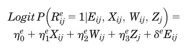
(eij), and then for both endpoints simultaneously. Let
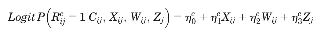
and similarly the probability of missing WTW,
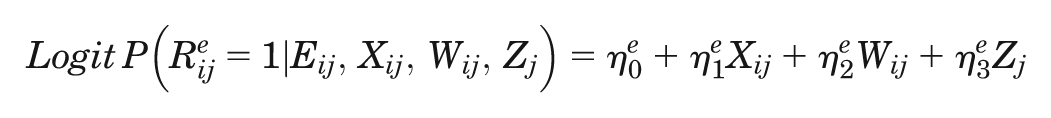
where
Description of scenarios
In Table 3, we list the scenarios considered. The choice of scenarios was informed by previous literature which suggests that the relative performance of the methods for handling missing data may differ according to the proportion of individuals with missing data11,15 and the type of variables that predict missingness (e.g., continuous or binary, individual-level or cluster-level). 30 We have also allowed for different missing data mechanisms, MCAR, MAR, and MNAR. 22 In particular, allowing the data to be MNAR was motivated by the general concern in CEA that probability of cost and outcome data may be conditional on the level of the endpoints.8,10,31 For example, in our case study it may be expected that women with lower WTW may be more likely to have missing WTW. Since the process utility endpoint, WTW, had lower ICC than the cost endpoint, we also hypothesized that there could be smaller differences between methods for handling the missing WTW data than for handling missing costs.15,17
Description of the Alternative Scenarios
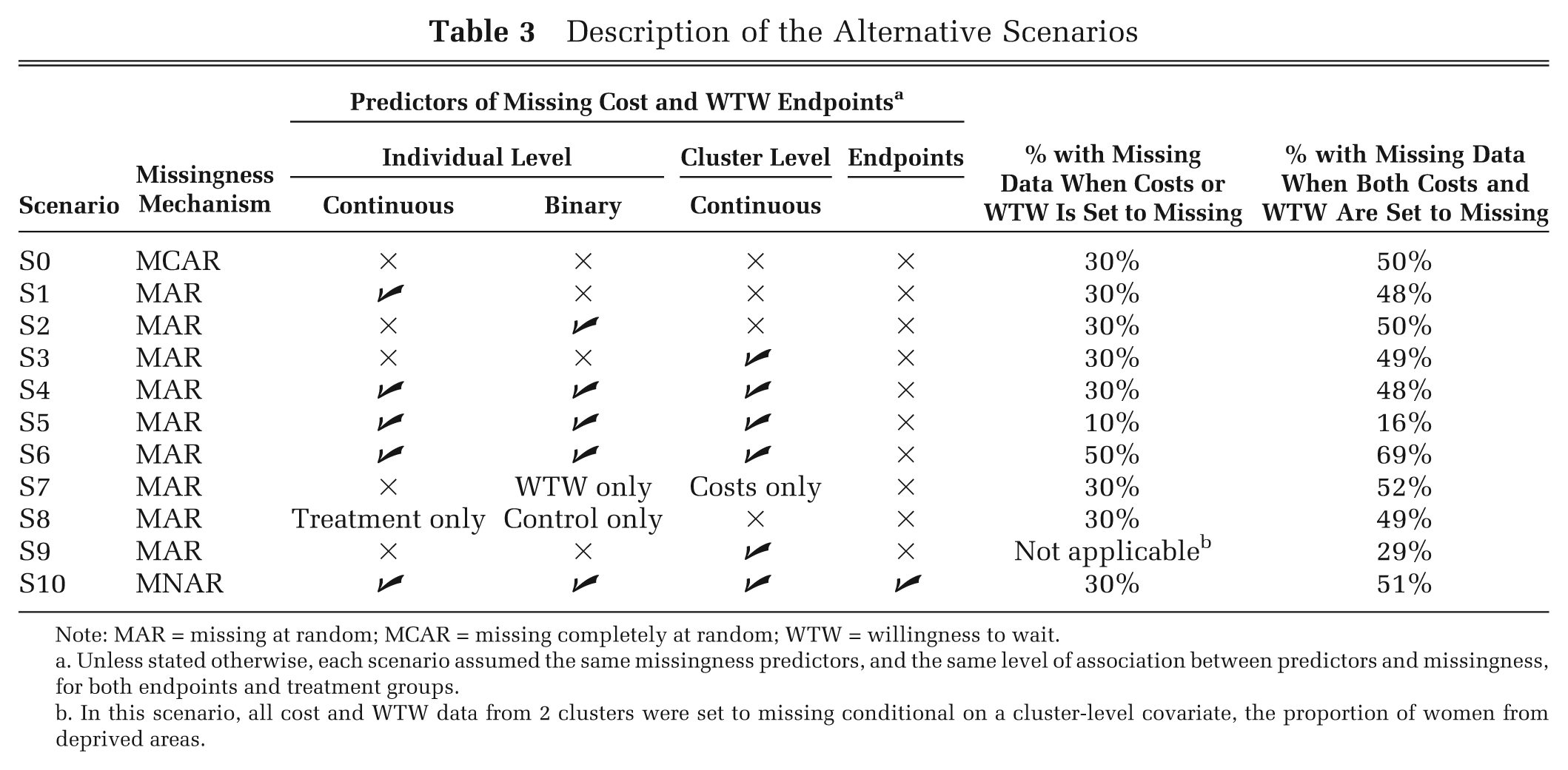
Note: MAR = missing at random; MCAR = missing completely at random; WTW = willingness to wait.
Unless stated otherwise, each scenario assumed the same missingness predictors, and the same level of association between predictors and missingness, for both endpoints and treatment groups.
In this scenario, all cost and WTW data from 2 clusters were set to missing conditional on a cluster-level covariate, the proportion of women from deprived areas.
We started by considering missing costs only and assuming that the proportion of observations
with missing data was 30%, a level typically seen in trial-based CEAs.8,10 In the first scenario (S0), we assumed that the missingness mechanism is MCAR, that
is, the missingness is independent of any observed or unobserved variable. Then, we allowed costs to
be MAR conditional on a continuous individual-level covariate, labor hours (S1); a binary
individual-level covariate, delivery mode (S2); a continuous cluster-level covariate, size of the
randomized cluster (S3); and then all 3 covariates (S4). For these scenarios, we followed previous
simulation studies32,33 and set the values for
We then conducted sensitivity analyses (scenarios S5–S10) that considered further circumstances faced by CEAs that use CRTs where the relative performance of the methods may be anticipated to differ. We considered low (S5) and high (S6) proportions of missing data and different missingness predictors by endpoint (S7) and by treatment arm (S8), and we set 2 whole clusters to have unobserved endpoints conditional on a continuous cluster-level covariate (S9). In the final scenario (S10), we allowed for the data to be MNAR by setting the probability of costs and WTW being missing to be dependent on the level of the endpoints as follows:
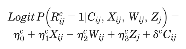
where
Implementation
For the imputation model, we followed general recommendations and took an inclusive approach to variable selection by including all covariates associated with either endpoint in either treatment group.23,25,34 In each scenario, we included all 5 individual-level covariates: delivery mode, number of previous hospital visits, mobility status, type of pain relief, and labor hours; and all 3 cluster-level covariates: size of the randomized cluster, size of the maternity unit, and proportion of women from deprived areas. Hence, the imputation model included covariates beyond those used to simulate the missing data. We specified joint models for the cost and WTW endpoints, separately for each treatment arm, and costs were log-transformed prior to imputation. We used the R packages “mice” 35 and “pan” 19 for the single-level and multilevel MI, respectively. We followed methodological guidance12,23 and imputed M = 10 data sets in each scenario but allowed M = 50 in the sensitivity analyses.
For each missing data approach, we estimated incremental cost and WTW with a BVN multilevel model (MLM) that assumed constant variances across clusters, 5 and we calculated the INB from the resultant parameter estimates. We assumed that there were no systematic imbalances in the baseline covariates, and we estimated linear additive treatment effects for both costs and WTW. For both MI methods, estimates were obtained by applying the MLM to each M imputed data set. These M = 10 estimates were then combined by Rubin's rules 22 to obtain MI estimates and standard errors.
In each scenario, we reported the mean (standard error) estimates for each method compared with
the corresponding estimates from the fully observed data, defined as the “true” estimates. We
reported the relative performance of each method as the percentage differences in the mean estimates
versus the true estimates. For example, the percentage mean differences (d) in the
INB were calculated as
Results
Missing Costs or WTW
In Table 4 (third column) we report
means and standard errors of the incremental cost across scenarios in which 30% of women had missing
costs. When costs were MCAR, all methods provided incremental costs similar to the true estimates
obtained from the fully observed data. Under MAR, CCA gave point estimates that differed from the
true incremental cost. In this setting with only the cost endpoint missing, the imputation
approaches used information from the fully observed WTW endpoint, which was highly correlated with
the costs (
Incremental Cost with 30% Missing Costs, and Incremental WTW with 30% Missing WTW, for CCA, Single-Level MI, and Multilevel MI
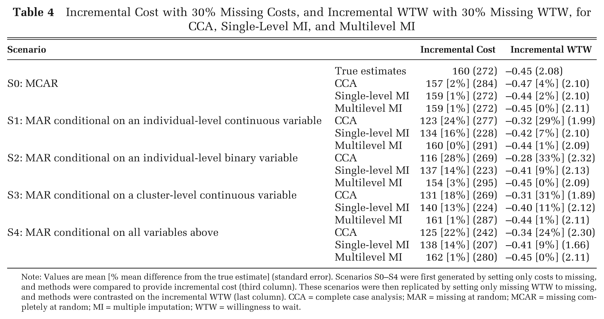
Note: Values are mean [% mean difference from the true estimate] (standard error). Scenarios S0–S4 were first generated by setting only costs to missing, and methods were compared to provide incremental cost (third column). These scenarios were then replicated by setting only missing WTW to missing, and methods were contrasted on the incremental WTW (last column). CCA = complete case analysis; MAR = missing at random; MCAR = missing completely at random; MI = multiple imputation; WTW = willingness to wait.
Table 4 (last column) also presents the results for the same scenarios but assuming that only WTW was missing (30%). Between-method differences were similar to those for missing costs; multilevel MI provided WTW estimates consistently closer to the true estimates. However, for the WTW endpoint, a relatively low proportion of the variation was at the cluster level (ICC = 0.03), and so the single-level MI gave estimates that were somewhat closer to the true estimates than for the previous scenarios with missing costs. For some scenarios, CCA reported standard errors that differed from the true standard errors. This was because the subsamples with observed data happened to have more or less variability in their WTW or cost data than those observations whose endpoints were set to missing.
Missing Costs and WTW
In Table 5 we report incremental cost, incremental WTW, and INB assuming that for 30% of women either costs or WTW was MAR; the proportion of women with missing data for either endpoint was around 50% (Table 3) and for both endpoints was 10%. CCA and single-level MI provided point estimates of the INB that diverged from the true INB, and single-level MI also provided smaller standard errors. The divergence between the true and estimated INBs reflected those for the incremental costs and WTW, which were generally higher than for the previous scenarios where only one endpoint was set to missing (Table 4). Here, a higher proportion of women were missing either endpoint (approximately 50% v. 30%), and for those women missing both endpoints the imputation was solely reliant on the covariate information. The multilevel MI gave point estimates and standard errors consistently close to the true INB.
Incremental Cost, Incremental WTW, and INB According to Method, across Different Scenarios with Costs and WTW Missing
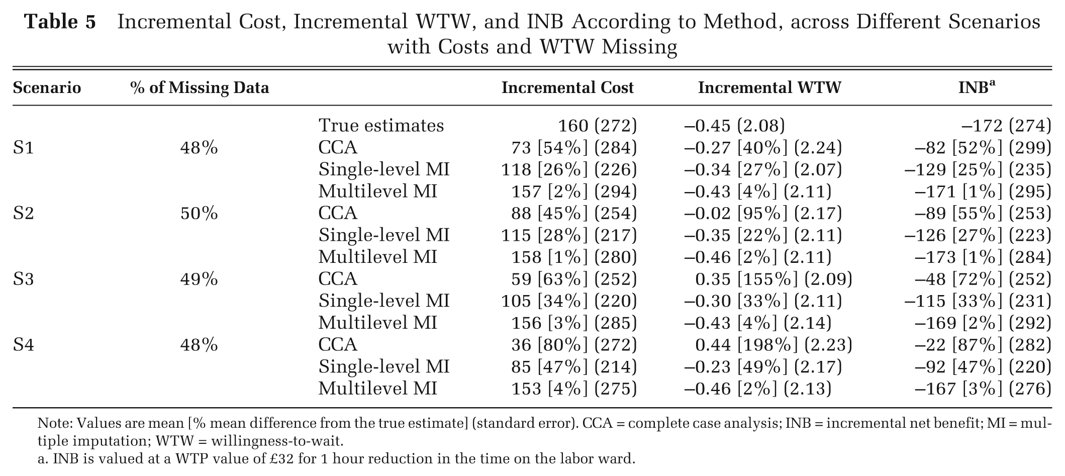
Note: Values are mean [% mean difference from the true estimate] (standard error). CCA = complete case analysis; INB = incremental net benefit; MI = multiple imputation; WTW = willingness-to-wait.
INB is valued at a WTP value of £32 for 1 hour reduction in the time on the labor ward.
The results were similar when we assumed low (correlation = 0.2) or high (correlation = 0.7) levels of association between the covariates and the probability of missingness, when the number of imputations was increased to 50.
The CEACs illustrated for scenario S4 (Figure 1) showed that multilevel MI provided estimates closest to the true probability that the intervention is cost-effective across a wide range of WTP thresholds considered.
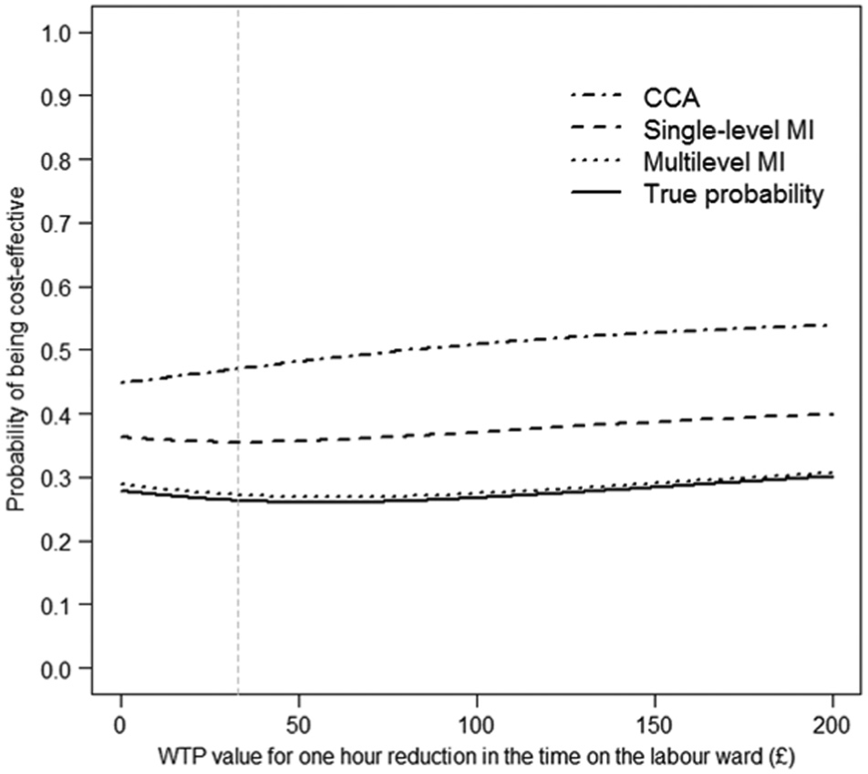
Cost-effectiveness acceptability curves according to method, using estimates from scenario S4. CCA = complete case analysis; MI = multiple imputation; WTP = willingness to pay.
Sensitivity Analyses
Both CCA and single-level MI provided divergent point estimates from the true estimates, even in circumstances where each endpoint was missing for only 10% of women (84% complete cases) (Table 6). These estimates were further from the true estimates when 50% of observations were missing either endpoint (31% complete cases). By contrast, multilevel MI reported estimates closer to those from the fully observed data. Similar between-method differences were reported when we allowed for different predictors by endpoint (S7) and by randomized arm (S8) and when the costs and WTW of all the patients from 2 clusters were set to missing (S9).
INB (WTP value: £32 per hour) for Each Method across Sensitivity Analysis Scenarios
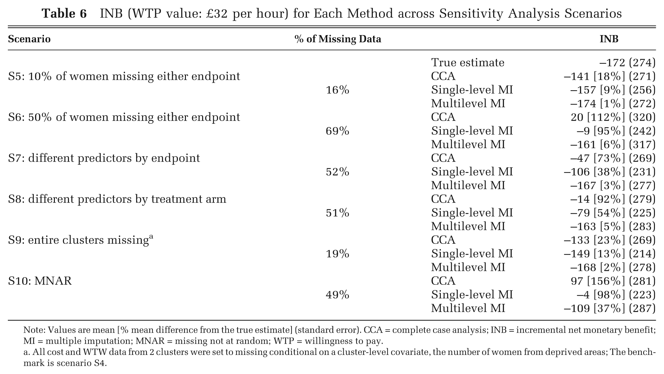
Note: Values are mean [% mean difference from the true estimate] (standard error). CCA = complete case analysis; INB = incremental net monetary benefit; MI = multiple imputation; MNAR = missing not at random; WTP = willingness to pay.
All cost and WTW data from 2 clusters were set to missing conditional on a cluster-level covariate, the number of women from deprived areas; The benchmark is scenario S4.
Figure 2 illustrates the relative performance of each method under MNAR scenarios with increasing levels of association between the fully observed endpoints and the probability of missingness. Here, multilevel MI provides INB estimates that were relatively close to the true INB when the correlation between the value of the endpoint and its missingness was fairly weak (correlation ≤ 0.2). Once we assumed a stronger relationship between the endpoints and the probability of missingness (correlation ≥ 0.4), none of the methods gave accurate estimates, but those from the multilevel MI were still closest to the true estimates.
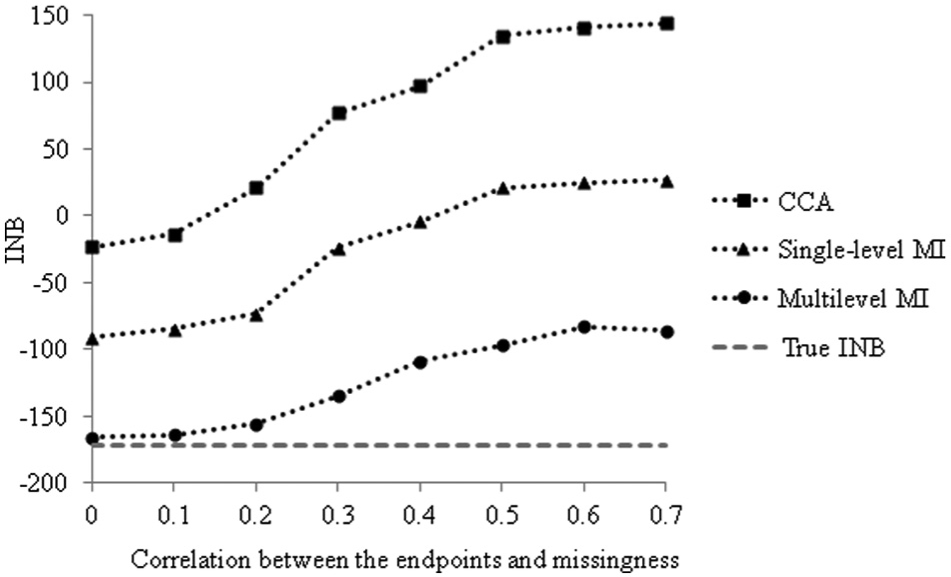
INB (WTP value: £32 per hour) according to method for MNAR scenarios (the benchmark is S4) at increasing levels of association between endpoints and missingness. CCA = complete case analysis; INB = incremental net monetary benefit; MI = multiple imputation; MNAR = missing not at random; WTP = willingness to pay.
Discussion
This paper presents a multilevel MI approach for handling missing data in CEAs that use hierarchical data. This method is grounded on methodological guidance in the biostatistics literature which recommends its use for the analysis of missing data in hierarchical settings.12,16,19,23 In the context of a CEA alongside a CRT, we find that multilevel MI gives point estimates of cost-effectiveness and standard errors consistently close to those from the fully observed data. We therefore recommend that future studies adopt this approach for handling missing data in CEAs that use cluster trials, irrespective of the prevalence of missing data. CCA provides point estimates that are divergent from those of the fully observed data across all scenarios, and its use is discouraged. The estimates from the single-level MI are closer to the true estimates in less challenging settings, such as when the ICC is low and only one endpoint has missing data. However, in most scenarios this MI approach leads to misleading point estimates and standard errors. These scenarios include those when the cost endpoint, which had a higher ICC, is missing and when a higher proportion of patients are missing either endpoint.
Single-level MI does not recognize that observations within each cluster may be correlated, and it assumes that there is more information than there actually is and, hence, that the resultant precision of the resultant estimates is overstated. Our results suggest that approaches that ignore the clustering not only exaggerate the precision but can also lead to inappropriate point estimates. The way that single-level MI weights individuals within each cluster differs from that of multilevel MI. The resultant point estimates can differ between single-level and multilevel MI approaches when the randomized clusters are of different size and the relationship between cluster size and either endpoint differs by treatment arm. Previous work has shown that in such circumstances, multilevel versus single-level analysis models can give different point estimates.6,36 A previous simulation study for handling missing univariate endpoint data in CRTs also found that single-level MI underestimates the uncertainty around the estimates. 15
A previous paper proposed multilevel MI for CEAs that use cluster trials in a reanalysis of a single case study. 20 We extend this work by assessing the methods’ performance against estimates obtained from fully observed cases. This allowed the methods to be compared across a wide range of circumstances typically encountered in CEAs that use CRTs. 18 We found that unless data are MCAR, which is unlikely, CCA and the single-level MI approach appear inappropriate for studies with clustered data. The multilevel MI approach is compatible with MLMs for handling cost-effectiveness data with a multilevel structure.2,3,5 Previous simulations studies5,36 showed that MLMs developed for CEAs that use CRTs performed relatively well even with a small number of clusters (3 per arm). In our case study, which had 7 clusters per arm, the use of multilevel MI for handling the missing data combined with MLMs for the analysis provided both point estimates and uncertainty measures close to the true values.
Previous papers have proposed single-level MI approaches for handling missing data in CEAs.7–11 Simulations have shown that single-level MI can perform relatively well with a single endpoint and when the data are not hierarchical.10,11 More generally, CEAs based on patient-level data tend to use hierarchical designs such as multicenter and cluster trials, where the data can be anticipated to have a multilevel structure. The multilevel MI approach proposed, although illustrated in the context of a CEA from a CRT, can be extended to other hierarchical settings such as multicenter or multinational studies.
While multilevel MI has been proposed more generally for handling missing data that have a hierarchical structure,12,16,19 the CEA context brings additional challenges for the method. In this setting, methods need to recognize that the probability that one endpoint is missing may be dependent on the other endpoint; for example, patients in worse health may be less likely to return resource use questionnaires. Here, we recognized this by considering joint imputation models for missing costs and WTW (Models 1 and 2 above), which used the information of the observed endpoint to impute the missing endpoint. In addition, we acknowledged that costs tend to have a right-skewed distribution by log-transforming them before any imputation and back-transforming the data after imputation.8,11 As data were back-transformed before the analytical models were applied, this avoided the retransformation problem that can occur when one is back-transforming estimates from log-normal endpoint models. 37 For the analytical model, we considered bivariate normal MLMs, which have been shown to perform well across different circumstances in CEAs that use CRTs, including when costs are skewed.5,6,36
Our analysis compared a multilevel MI approach that used a joint normal distribution with a commonly used single-level MI procedure that uses a full conditional specification (sometimes called the chained equations approach). 35 When instead we implemented both single-level MI and multilevel MI using the chained equations approach, differences in the estimates between the single-level and multilevel approach remained the same. The multilevel MI approach can be readily implemented in available software; we chose to use the R package and to append code to help disseminate the method (Appendix 2), but other available software options include the mi macro in MLwiN 12 and the REALCOM-impute macros. 38
MI methods, like other principled approaches for handling missing data, such as maximum likelihood estimation and full-Bayesian analyses (estimated via MCMC), assume that the data are MAR. In practice, data may be missing dependent on unobserved factors (e.g., patient lifestyle factors); that is, the data may be MNAR. This paper considered settings in which data were assumed to be MNAR, and it showed that cost-effectiveness results by either MI approach were sensitive to departures from the MAR. In this case study, multilevel MI reported cost-effectiveness estimates that were closest to the true estimates across the alternative MNAR scenarios. However, it is important for future CEAs to conduct structural sensitivity analyses to consider how to handle possible MNAR mechanisms. MI approaches under MAR are amenable to such sensitivity analyses, and this is an ongoing area of methodological research. 39
This paper has some limitations. First, we did not undertake a full simulation study, which would have allowed metrics such as bias, mean squared error, and confidence interval coverage to be compared across the methods. Previous simulation studies15,17 have suggested that multilevel MI outperforms single-level MI with clustered data, and either approach can reduce bias versus CCA. Here, we chose a design that allowed us to compare the different methods across a range of plausible mechanisms, which gave rise to incomplete data in a typical CEA alongside a CRT. By taking this approach, we could examine the implications of the choice of method on cost-effectiveness estimates for alternative missing data mechanisms. These findings will help inform a future simulation study. Second, the paper has taken data from a single case study and investigated missing data for costs and a measure of process utility. More generally, the missing data may take different forms to those considered here; for example, the endpoint may be binary or time to event, and the pattern of the missing data may be more complex (e.g., different components of resource use). Third, our analyses were based on a single replication of the missing data, but when we conducted 1000 replications for particular scenarios, the findings were unchanged. Fourth, this study contrasted multilevel MI with single-level MI, which has been previously proposed for CEAs, and CCA, an approach commonly taken in applied studies. However, other methods for handling missing data in CEAs, such as inverse probability weighting 23 and full-Bayesian approaches, 40 could also be extended to allow for clustering.
The findings from this paper provoke several areas for further research. Future studies could consider the relative performance of a broader range of methods in more general circumstances faced by CEAs. In particular, it would be useful to contrast full-Bayesian approaches with multilevel MI for handling other complex structures, for example, CEAs that have longitudinal data. Here, it would be interesting to contrast the potential flexibility that Bayesian approaches may afford with respect to exploiting external data, with the additional requirements of specifying prior distributions. Second, further work is needed to develop approaches for exploring the sensitivity the cost-effectiveness results to departures from the MAR assumption, by considering a range of possible MNAR mechanisms.23,39,41 Such approaches can allow analysts to present decision makers with a fuller representation of the uncertainty that surrounds the CEA results, to facilitate a sounder basis for future decisions.
Footnotes
Acknowledgements
The authors are grateful to Graham Scotland and Paul McNamee, for providing access to the Maternity data set, and to Simon Thompson, James Carpenter, Simon Dixon, Zia Sadique, and John Cairns for their helpful comments.
KDO and RG acknowledge financial support from a UK Medical Research Council grant. The views expressed are those of the authors and may not reflect those of the funder.
*
ICCs are estimated using a small-sample adjustment due to the small number of clusters per treatment arm. 27
†
For example, the usual Pearson correlation coefficient between a continuous covariate
(X) and the binary missingness indicator (R) was calculated as
References
Supplementary Material
Please find the following supplemental material available below.
For Open Access articles published under a Creative Commons License, all supplemental material carries the same license as the article it is associated with.
For non-Open Access articles published, all supplemental material carries a non-exclusive license, and permission requests for re-use of supplemental material or any part of supplemental material shall be sent directly to the copyright owner as specified in the copyright notice associated with the article.