Microvascular plasticity in mouse stroke model recovery: Anatomy statistics,dynamics measured by longitudinal in vivo two-photon angiography,network vectorization

Abstract

This manuscript quantitatively investigates remodeling dynamics of the cortical microvascular network (thousands of connected capillaries) following photothrombotic ischemia (cubic millimeter volume, imaged weekly) using a novel in vivo two-photon angiography and high throughput vascular vectorization method. The results suggest distinct temporal patterns of cerebrovascular plasticity, with acute remodeling peaking at one week post-stroke. The network architecture then gradually stabilizes, returning to a new steady state after four weeks. These findings align with previous literature on neuronal plasticity, highlighting the correlation between neuronal and neurovascular remodeling. Quantitative analysis of neurovascular networks using length- and strand-based statistical measures reveals intricate changes in network anatomy and topology. The distance and strand-length statistics show significant alterations, with a peak of plasticity observed at one week post-stroke, followed by a gradual return to baseline. The orientation statistic plasticity peaks at two weeks, gradually approaching the (conserved across subjects) stroke signature. The underlying mechanism of the vascular response (angiogenesis vs. tissue deformation), however, is yet unexplored. Overall, the combination of chronic two-photon angiography, vascular vectorization, reconstruction/visualization, and statistical analysis enables both qualitative and quantitative assessments of neurovascular remodeling dynamics, demonstrating a method for investigating cortical microvascular network disorders and the therapeutic modes of action thereof.

Introduction

The cerebrovasculature is a highly dense network of blood vessels that support metabolic activity in the brain through neurovascular coupling. ¹ With the strong relationship between neuronal function and the cerebrovasculature, perturbations to the vascular structure can result in profound functional consequences. Due to neurovascular coupling, it is reasonable to hypothesize that neurovascular plasticity and neuronal plasticity would be highly correlated. ² Therefore, it is paramount to thoroughly understand the intricacies of both healthy and unhealthy cerebrovascular structure and plasticity.

Endpoint histological studies have revealed many conditions where vascular structure deviates from normal, including aging,^{3 –5} deafness, ⁶ hypoxia,^{7 –9} neurodegenerative disease, ¹⁰ and stroke. ¹¹ While endpoint studies have elucidated many important biological phenomena, they naturally limit the temporal sampling to once per subject. Conclusions are therefore only drawn across specimens which obscures results and complicates findings. Additionally, the vascular structure after preservation does not perfectly represent the in vivo state which then requires careful calibration of microvessel diameter. ¹²

Many issues of endpoint studies in rodents are addressed with chronic in vivo imaging making use of two-photon microscopy (2PM). This technique has proved useful for investigating how aging, ¹³ physical activity, ¹⁴ hypoxia, ⁹ and ischemia^15,16 affects cerebrovascular plasticity in individual mice. However, there are restrictions to the amount of vasculature that can be imaged through 2PM due to limitations in both the lateral field of view (FOV) and penetration depth of excitation light. Furthermore, many conclusions from these studies rely on evaluating images manually, further decreasing the already limited volumes of vasculature investigators can reasonably analyze. Relationships between stimuli and cerebrovascular plasticity are not always clear, and studies require large sample sizes to establish statistical significance. Many endpoint studies in rodents reveal that maintained physical activity encourages at least temporary increases in microvascular density in the motor cortex and hippocampus.^{17 –21} However, no difference was identified between mice housed with monitored exercise wheels and a control group in a chronic in vivo evaluation performed by Cudmore et al. ¹⁴ using manual vessel tracing. It could prove beneficial to perform similar studies using an automated vectorization method to efficiently evaluate larger vascular networks, ultimately increasing the statistical power of any findings.

Vectorization of microcirculatory angiograms enables three-dimensional reconstruction and quantitative comparison of samples, increasing the volumes of data and number of statistics that can be investigated. With images acquired through ex vivo methods, which are often of a very high quality, researchers can skeletonize datasets following binarization.^{22 –25} These methods have been used to reconstruct an entire mouse brain, ²⁶ to enable blood flow simulations,^27,28 and to show organizational similarities in vascular structures across species. ²⁹

Vectorization can be more difficult with in vivo neurovascular images, however, as these often suffer from low signal to background ratio (SBR) and local fluctuations in image quality. The vectorization strategy must be robust enough to combat these issues. To this point, groups have used in vivo vectorization to study network topology,^{30 –32} for simulating laser speckle contrast imaging (LSCI),^33,34 and for evaluating experimental imaging methods.^35,36 Here we expand upon these and present vectorizations of much larger in vivo tissue volumes in both ischemic and control mice.

We first show an in vivo imaging strategy that covers large tissue volumes (exceeding 1 cubic millimeter) in the mouse brain at the resolution of capillaries (1.5 micrometers in x-y, 3 in z) and then demonstrate a vectorization strategy that can efficiently vectorize these entire volumes. Finally, we illustrate that the high-performance vectorization strategy can accurately and efficiently compare the anatomy of the intricate microvascular network across multiple subjects in a longitudinal (five time points, once per week) stroke model study. To our knowledge, this is the first time that automated vectorization techniques were used to statistically analyze in vivo neurovasculature over a volume of this size in a longitudinal manner. Other studies have either analyzed vascular morphometrics through manual methods,^{9,13 –16,37} or covered much smaller fields of view when automated methods were employed.^38,39 Our imaging and vectorization methods enable a study of cerebral vascular plasticity with high statistical significance and serve as an example for future animal model investigations into potential therapeutics to treat neurodegenerative diseases and neural injuries.

Materials and methods

Experimental design

The experimental methods are graphically explained in Figure 1. Laser speckle contrast imaging (LSCI) was initially performed three weeks after cranial window implantation and used to evaluate craniotomy quality. Mice were then imaged with both multi-exposure speckle imaging (MESI) and two-photon microscopy (2PM) to get initial (week 0) anatomical and blood flow time points. The following day photothrombotic ischemia was induced in six of the mice with vessel structures which appeared optimal for occlusion. Of these, one died and 2PM image quality drastically lowered in two others, leaving three for longitudinal analysis. In these, weekly 2PM and MESI was performed for four weeks resulting in five total time points (weeks 0–4) per stroke model subject. This ultimately yielded three baseline and twelve post-stroke image sets for vectorization and statistical analysis. An additional MESI time point was acquired two days after ischemia to better visualize the immediate recovery stage following photothrombosis. Additionally, in three healthy control mice where photothrombosis was not performed, 2PM imaging was performed bi-weekly over the course of four weeks resulting in images from three time points (weeks 0, 2, 4). Table S1 summarizes the two study groups, providing the time points at which they were imaged through 2PM and their designations (A, C, and E for stoke model mice, and B, D, and F for healthy control mice).

Figure 1.

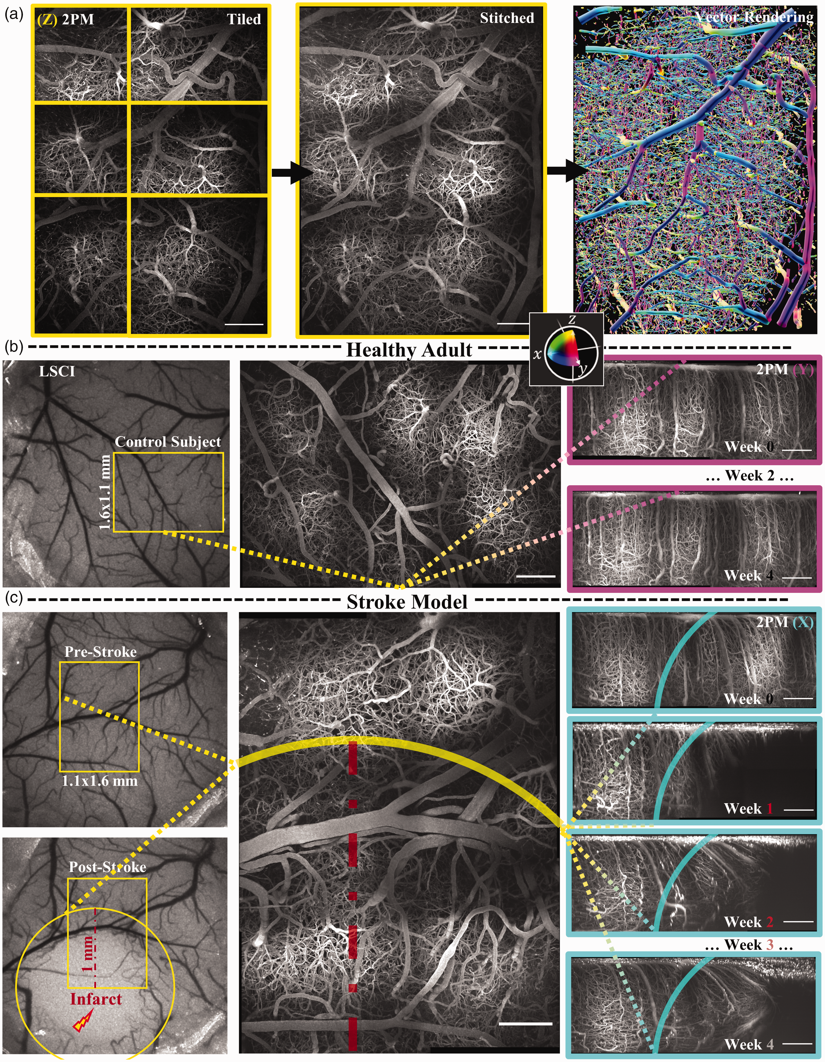
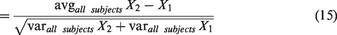
Experimental Methods: (a) Mouse cortex is imaged in vivo through a cranial window using a tiling protocol to cover as large of a volume as possible in a single imaging session. The stitched image is vectorized using the SLAVV software for reconstruction, visualization, and statistical analysis. The vessel directions (as well as the borders of the 2PM images and the ROI borders) are color-coded with respect to their alignment with the imaging coordinate system: (xyz<->CMY). (b) LSCI is used to orient the 2PM imaging session to reproducibly image the same (∼1 mm³) volume longitudinally over several imaging sessions at two-week intervals and at a depth greater than 600 micrometers. Displayed is an orthographic projection in the (optical) z-axis of a tiled image volume of a healthy control subject. Lateral orthographic projections show the longitudinal imaging reproducibility and (c) the longitudinal experiment is repeated around a photothrombotic injury. The infarct appears to be contained to a (yellow) circle with a radius of approximately 1 mm in the LSCI post-stroke image. The x-projected 2PM image reveals that a (transparent cyan) spherical ROI beneath the surface approximates the shape of the infarct. Scale bars are 200 μm.

Mouse craniotomy

All procedures followed the Guidelines for Surgical and Anesthetic Procedures in Rodents set by the University of Texas Institutional Animal Care and Use Committee, which approved this study. All results were reported in compliance with the ARRIVE (Animal Research: Reporting In Vivo Experiments) guidelines. Cranial windows were implanted on anesthetized (isoflurane, 1.5%, 0.6–0.8 liters per minute, LPM) mice (C57BL/6, male, between three and six months of age) while body temperature was maintained with a heating pad using a procedure similar to ones previously described.^16,40,41 Carprofen was injected at 10 mg/kg prior to surgery. A skull portion slightly exceeding 5 mm in diameter over the motor cortex of the right hemisphere was then removed and a 5 mm diameter glass coverslip was implanted in its place using cyanoacrylate and dental cement. Mice were housed 2–5 per cage, and were allowed to heal for three weeks prior to optical imaging and photothrombosis.

Photothrombosis

Ischemia was induced through injecting 0.15 ml of 15 mg/ml rose bengal retro-orbitally and irradiating a penetrating arteriole branching from the middle cerebral artery for 15 minutes using a 532 nm, 20 mW laser source focused to a ∼300 μm diameter spot size.^42,43 Mice were anesthetized with isoflurane (1.5%, 0.6–0.8 LPM) and body temperature was maintained with a heating pad during photothrombosis. Pial anatomy was visualized using LSCI during the procedure to select which artery to target and to confirm occlusion. Anonymization of the subjects to the researchers was practically impossible, because the presence of the stroke was obvious in the images.

Laser speckle contrast imaging and multi-exposure speckle imaging

LSCI was performed in mice anesthetized with isoflurane (1.5%, 0.6–0.8 LPM) using a system described previously. ⁴⁴ In imaging sessions where blood flow was evaluated, sequences of 15 laser speckle contrast images were acquired at different exposure times to perform MESI, an extension of LSCI which allows for more accurate measurements of cerebral blood flow (CBF). The brain surface was imaged onto a camera and illuminated using a 785 nm laser diode to provide light for imaging. LSCI was also used as a feedback mechanism to orient the brain tilt prior to 2PM imaging sessions to encourage longitudinal reproducibility through imaging the same tissue volume.

Two-photon fluorescence imaging

2PM was performed immediately after MESI on imaging days. 100 μl of 70 kDa dextran-conjugated Texas red diluted in saline at a 5% w/v ratio was injected retro-orbitally and excited using a custom ytterbium fiber amplifier (λ = 1060 nm, 80 MHz repetition rate). ⁴⁵ The microscope used a resonant scanner to decrease acquisition time. Six stacks exceeding a 600 μm depth, 3 μm step size were acquired in adjacent, tiled regions and stitched together (Figure 1(a)). Final images had approximately a 1.6 × 1.1 × 0.6 mm³ field of view (Figure 1(b) and (c)), resulting in a volume exceeding 1 mm³. Pial architecture was used to image the same region at each time point.

Vascular vectorization

2PM volumetric angiographs were vectorized using the Segmentation-less Automated Vascular Vectorization (SLAVV) software in MATLAB ³¹ with two notable additions to improve throughput: (1) Machine learning assisted the manual curation task (2) A maximum resolution constraint was imposed to improve the computational efficiency for the larger vessels in the image. Although the machine-assisted curation proved extremely helpful for the capillary bed, some of the larger surface and descending vessels were manually curated into agreement with the underlying 2PM angiograph for display purposes only. Fully automated vascular vectorization enabled all of the statistical analyses, reconstructions, and other visualizations.

Standardized, fully automated vectorization with machine-learned curation

In an effort to increase the throughput of, remove bias from, and standardize the statistical analysis across all subjects, the manual task of curating the extracted vertices and edges was fully automated using simple machine learning classifiers trained on human curations of healthy subjects using dimensionless features of gradient and curvature/vesselness (normalized by signal variance as required to achieve a dimensionless quantity). A threshold of 70% classification probability was chosen for the vertices. The edges were thresholded at 50% on a single unitless feature of local curvature variation. In this way, all of the subjects were processed in a consistent, fully automated way with a similar classification sensitivity and specificity for the vertex and edge objects.

Statistical analysis of vascular networks

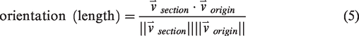
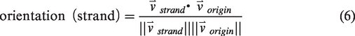
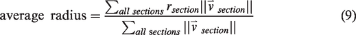
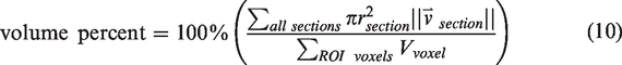
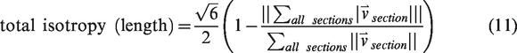
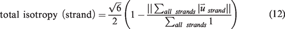
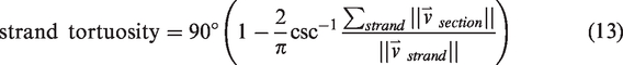
The definitions of the statistics of interest in this study are given in equations (1) to (16). The vectorized vascular network is idealized as a collection of short, contiguous, cylindrical “sections,” which are partitioned into the set of non-bifurcating, 1-D traces “strands,” as demonstrated in Figure 2(e). Sections provide a nearly continuous view of the vessels and share the length of the voxel, whereas strands respect the topology of the network (they do not pass through vessel junctions) so they allow for network topology measurements (number of strands, strand lengths, tortuosities). Under this idealization, anatomical statistics (vessel length, distance from ROI center, and orientation to ROI center) were calculated from the vectorized reconstructions of angiographs in MATLAB using the SLAVV software. Statistical distributions (i.e. spectra) of the vascular anatomy served to quantitatively characterize the vascular networks. Where possible, both strand- and section-based statistical (distance, orientation) distributions were generated. Strand-basis statistical (average radius, length, and tortuosity) distributions were generated to compare to the known previous study of microvascular network topology. ³⁰ Section-basis statistics, which are weighted by length, were also used in the present application due to their simpler definitions, larger sample sizes, and better reproducibility. The following equations define the statistics of interest presented herein.

$$\begin{array}{c}s\mathrm{ection} \mathrm{length}=‖{\stackrel{\rightharpoonup }{v}}_{\mathit{section}}‖\end{array}$$

(1)

$$\mathrm{total} \mathrm{length}=\sum _{\mathit{all}\mathrm{ }\mathit{sections}}‖{\stackrel{\rightharpoonup }{v}}_{\mathit{section}}‖$$

(2)

$$\mathrm{strand} \mathrm{length}=\sum _{\mathit{strand}}‖{\stackrel{\rightharpoonup }{v}}_{\mathit{section}}‖$$

(3)

$$\begin{array}{c}\mathrm{section}/\mathrm{strand} \mathrm{distance}=‖{\stackrel{\rightharpoonup }{v}}_{\mathit{origin}}‖\end{array}$$

(4)

$$\begin{array}{c}\mathrm{orientation} \left(\mathrm{length}\right)=\frac{{\stackrel{\rightharpoonup }{v}}_{\mathit{section}}·{\stackrel{\rightharpoonup }{v}}_{\mathit{origin}}}{‖{\stackrel{\rightharpoonup }{v}}_{\mathit{section}}‖‖{\stackrel{\rightharpoonup }{v}}_{\mathit{origin}}‖}\end{array}$$

(5)

$$\begin{array}{c}\mathrm{orientation} \left(\mathrm{strand}\right)=\frac{{\stackrel{\rightharpoonup }{v}}_{\mathit{strand}}\bullet \mathrm{ }{\stackrel{\rightharpoonup }{\mathit{v}}}_{\mathit{origin}}}{‖{\stackrel{\rightharpoonup }{v}}_{\mathit{strand}}‖‖{\stackrel{\rightharpoonup }{v}}_{\mathit{origin}}‖}\end{array}$$

(6)

$$\mathrm{total} \mathrm{area}=\sum _{\mathit{all}\mathrm{\hspace{0.17em}\hspace{0.17em}}\mathit{sections}}2\pi r_{\mathit{section}}‖{\stackrel{\rightharpoonup }{v}}_{\mathit{section}}‖$$

(7)

$$\mathrm{total} \mathrm{volume}=\sum _{\mathit{all}\mathrm{\hspace{0.17em}\hspace{0.17em}}\mathit{sections}}\pi r_{\mathit{section}}^2‖{\stackrel{\rightharpoonup }{v}}_{\mathit{section}}‖$$

(8)

$$\begin{array}{c}\mathrm{average} \mathrm{radius}=\frac{\sum _{\mathit{all}\mathrm{\hspace{0.17em}\hspace{0.17em}}\mathit{sections}}{r}_{\mathit{section}}‖{\stackrel{\rightharpoonup }{v}}_{\mathit{section}}‖}{\sum _{\mathit{all}\mathrm{\hspace{0.17em}\hspace{0.17em}}\mathrm{s}\mathit{ections}}‖{\stackrel{\rightharpoonup }{v}}_{\mathit{section}}‖}\end{array}$$

(9)

$$\begin{array}{c}\mathrm{volume} \mathrm{percent}=100\%\left(\frac{\sum _{\mathit{all}\mathrm{\hspace{0.17em}\hspace{0.17em}}\mathit{sections}}\pi r_{\mathit{section}}^2‖{\stackrel{\rightharpoonup }{v}}_{\mathit{section}}‖}{\sum _{\mathit{ROI}\mathrm{ }\mathit{voxels}}{V}_{\mathit{voxel}}}\right)\end{array}$$

(10)

$$\begin{array}{c}\mathrm{total} \mathrm{isotropy} \left(\mathrm{length}\right)=\frac{\sqrt{6}}{2}\left(1-\frac{‖\sum _{\mathit{all}\mathrm{ }\mathit{sections}}\left|{\stackrel{\rightharpoonup }{v}}_{\mathit{section}}\right|‖}{\sum _{\mathit{all}\mathrm{ }\mathit{sections}}‖{\stackrel{\rightharpoonup }{v}}_{\mathit{section}}‖}\right)\end{array}$$

(11)

$$\begin{array}{c}\mathrm{total} \mathrm{isotropy} \left(\mathrm{strand}\right)=\frac{\sqrt{6}}{2}\left(1-\frac{‖\sum _{\mathit{all}\mathrm{ }\mathit{strands}}\left|{\stackrel{\rightharpoonup }{u}}_{\mathit{strand}}\right|‖}{\sum _{\mathit{all}\mathrm{ }\mathit{strands}}1}\right)\end{array}$$

(12)

$$\begin{array}{c}\mathrm{strand} \mathrm{tortuosity}=90°\left(1-\frac{2}{\pi }{\csc }^{-1}\frac{\sum _{\mathit{strand}}‖{\stackrel{\rightharpoonup }{v}}_{\mathit{section}}‖}{‖{\stackrel{\rightharpoonup }{v}}_{\mathit{strand}}‖}\right)\end{array}$$

(13)

$$\begin{array}{c}\mathrm{K}–\mathrm{S} \mathrm{test} \left(\mathrm{for} \mathrm{vector} \mathrm{statistic} \mathrm{x}\right)={\left.\left({\mathrm{CDF}}_2\left(x\right)-{\mathrm{CDF}}_1\left(x\right)\right)\right|}_{\underset{x}{\max }\left(\mathrm{abs}\left({\mathrm{CDF}}_2\left(x\right)-{\mathrm{CDF}}_1\left(x\right)\right)\right)}\end{array}$$

(14)

$$\begin{array}{c}\mathrm{z}–\mathrm{score} \left(\mathrm{for} \mathrm{summary} \mathrm{statistic} \mathrm{X}\right)\end{array}$$

$$=\frac{\underset{\mathit{all}\mathrm{ }\mathit{subjects}}{\mathrm{avg}}{X}_2-X_1}{\sqrt{\underset{\mathit{all}\mathrm{ }\mathit{subjects}}{\mathrm{var}}{X}_2+\underset{\mathit{all}\mathrm{ }\mathit{subjects}}{\mathrm{var}}{X}_1}}$$

(15)

$$\mathrm{z}\mathrm{–}\mathrm{score}\mathrm{ }\left(\mathrm{for}\mathrm{ }\mathrm{K}\mathrm{–}\mathrm{S}\mathrm{ }\mathrm{test}\mathrm{ }\mathrm{for}\mathrm{ }\mathrm{vector}\mathrm{ }\mathrm{statistc}\mathrm{ }\mathrm{x}\right)$$

$$=\frac{({\underset{\mathit{all}\mathrm{ }\mathit{subjects}}{{\mathrm{CDF}}_2}\left(x\right)-\underset{\mathit{all}\mathrm{ }\mathit{subjects}}{{\mathrm{CDF}}_1}\left(x\right))}_{\underset{x}{\max }\left(\mathrm{abs}\left({\mathrm{CDF}}_2\left(x\right)-{\mathrm{CDF}}_1\left(x\right)\right)\right)}}{\sqrt{\underset{\mathit{all}\mathrm{ }\mathit{subjects}}{\mathrm{avg}}\underset{x}{\max }{\left({\mathrm{CDF}}_2\left(x\right)\hspace{0.17em}\hspace{0.17em}-\hspace{0.17em}\hspace{0.17em}\hspace{0.17em}\underset{\mathit{all}\mathrm{ }\mathit{subjects}}{{\mathrm{CDF}}_2}\left(x\right)\right)}^2+\underset{\mathit{all}\mathrm{ }\mathit{subjects}}{\mathrm{avg}}\underset{x}{\max }{\left({\mathrm{CDF}}_1\left(x\right)-\underset{\mathit{all}\mathrm{ }\mathit{subjects}}{{\mathrm{CDF}}_1}\left(x\right)\right)}^2}}$$

(16)

where ${\stackrel{\rightharpoonup }{v}}_{\mathit{section}}$ is the vector representing the vessel section, ${\stackrel{\rightharpoonup }{v}}_{\mathit{strand}}$ the vessel strand vector (straight line from end to end), ${\stackrel{\rightharpoonup }{v}}_{\mathit{origin}}$ the vector from the ROI center to the vessel section or strand, $V_{\mathit{voxel}}$ the volume of a voxel, | - | the component-wise absolute value, ǁ - ǁ the vector magnitude (Pythagorean sum), and ${\stackrel{\rightharpoonup }{u}}_{\mathit{strand}}$ is the strand unit vector.

Figure 2.

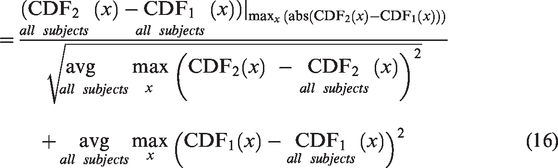
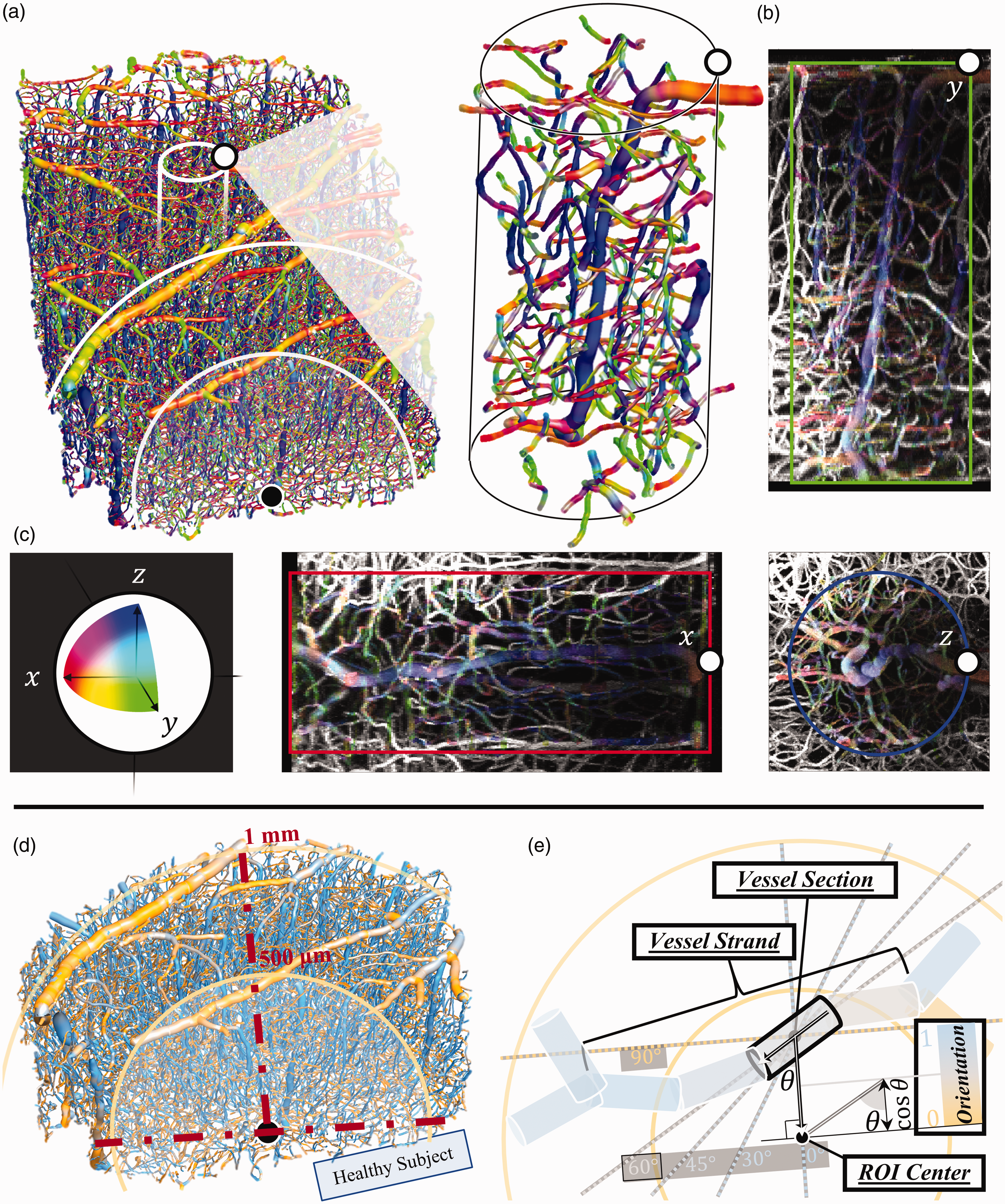
3D Directional Analysis: (a) A 3D perspective rendering shows the entire capillary network captured in the rectangular 2 × 3 tiled image. The 1 mm radius spherical ROI (500 micrometers line also shown) intersecting the near image boundary is used in the stroke model analysis. The pop-out magnifies an example penetrating (blue) vessel and surrounding vessel strands inside of a (250 micrometer diameter, 600 micrometer height) cylindrical ROI. (b) The strands from the cylindrical ROI overlay MIPs of a rectangular volume ROI of the raw 2PM image in x-, y-, and z-orthographic projections. (c) All vessel sections in the 3D reconstructions and those belonging to strands in the cylindrical ROI in the 2D projections (as well as the ROI borders) are color-coded according to their alignment to the axes of the imaging system (xyz<->RGB). (d) The 1 mm radius spherical ROI is magnified and re-colored according to its orientation to the ROI center and (e) visual legend describing the concepts of vessel strands vs. sections and the distance and orientation statistics with respect to the spherical ROI center.

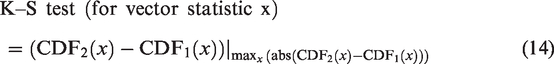
Statistical significance of longitudinal measurements

The Kolmogorov-Smirnov (K-S) test statistic (maximal absolute difference of CDFs) was used to summarize the differences between any two length-basis statistical distributions (normality not required or assumed) following a previous study. ³⁶ Changes in vascular structure were measured by comparing longitudinal differences with respect to (A) the previous time point and (B) the initial time point. Longitudinal baseline variations between imaging sessions from three healthy control subjects were established to estimate the statistical significance of the measured response of the vascular network to a photothrombotic event. A z-score was assigned to compare two conditions with respect to a given statistic, considering the inter-subject variations within each condition. We used the Jarque-Bera test for normality of the sample means, however due to the small number (n = 3) of means, it was difficult to prove their normality, however they are expected to be normally distributed by the central limit theorem. No formal t-test was performed in consideration of this limitation.

Directional analysis

Vessel directions are calculated by taking the derivative of the 3-space vessel centerline location with respect to the length coordinate along the vessel axis. Although vessel directions are color-encoded with respect to the canonical 3-space axes (Red, Green, Blue<->x, y, z) only on a section basis for demonstration purposes in Figure 2(a) to (c), for statistical purposes, the vessel orientations are color-encoded with respect to a spherical ROI center and summarized either on a section- or strand-basis as shown in Figure 2(d) and (e).

ROI selection

Regions of interest (ROIs) for the stroke model mice were selected to be concentric with the infarct center. Reproducible center point selection was achieved by registering all volumes to a stable reference feature of the vascular anatomy (far away from the infarct). For the healthy mouse, the ROI was selected to match the geometry of the stroke mouse ROI: a sphere with center at 650 µm depth intersecting the rectangular imaging volume. A cylindrical ROI was used in Figure 2(a) to (c) only to help explain the directional analysis in reference to the directions of the imaging system (with the cylinder and optical axes in the z-direction). The effective size of the infarct was variable between subjects and time points, however to simplify the analysis, all statistical analyses were spatially restricted to a spherical ROI as shown in Figure 2(d), and directional analysis was computed with respect to the ROI center. This size was chosen by visual inspection of all of the two-photon and LSCI images. A spherical radius of 1 millimeter appeared to capture the immediately affected tissue. Deeper analysis involving multidimensional histograms would be required to quantitatively and separately investigate the effect of distance from the infarct on the tissue dynamics.

Visualizations

Three-dimensional reconstructions of angiographs and two-dimensional overlays onto the maximum-intensity-projected original 2PM images were generated using the SLAVV software in MATLAB. A custom meshing algorithm was developed and used to generate the three-dimensional vascular network reconstruction at arbitrary resolution and with a user-specified color-coding. For the purposes of this manuscript, color-coding was chosen to display the direction of each short vessel section. Direction colors are coded with respect to the imaging system (Red,Green,Blue<->x,y,z) or with respect to a spherical ROI center (blue,yellow<->pointed toward the center, pointed tangentially to the spherical surface).

Results

Large-volume, 2PM in vivo angiography enables longitudinal stroke model vectorization

The imaging workflow visually described in Figure 1 enables reproducible vascular vectorization. LSCI (Figure 1(b) and (c), left side) was helpful in guiding photothrombotic stroke and in orienting the mouse brain for two-photon microscopy imaging sessions (Figure 1(b) and (c), right side). Time-lapse volumetric images of the peri-infarct region were acquired with high quality and reproducibility to study the response of the affected neurovascular network to photothrombosis. The lateral orthographic projection time-lapse shown on the right side of Figure 1(c) shows the qualitative changes to the vascular network as well as to the image itself near the infarct. An animation from such projections was produced to demonstrate the dynamic changes in vasculature following stroke (Supplementary Animation 1). Image quality decreases (spatially and temporally) near the infarct with a loss of signal and an increase in background. Vessels very close (<500 μm) to the infarct center disappear, while those nearby (<1 mm) appear to be reoriented and pulled toward the infarct center during recovery.

Directional analysis helps visualize neuro-microvascular networks

The directions of the vessels were color-encoded in certain visualizations to help conceptualize the complexity of the cortical microvascular network. The color-coding helps the image viewer appreciate the anisotropy of the vascular network, and it also facilitates vectorization performance evaluation. In Figures 1(a) and 2(a) to (c), the reconstructed color-coding highlights the vessels which are vertical (z-) as well as those which are aligned to the x- and y-axes of the imaging system. Figure 2(a) shows the strand objects from an example cylindrical ROI (not used for analysis) extracted from a larger two-photon imaging volume. Figure 2(b) shows the agreement (within the cylindrical ROI) between the original (projected) two-photon image with the vectorized reconstruction color-coded by three-dimensional direction. The central vertical vessel featured in the vectorized reconstruction can be clearly seen in blue in all three orthographic projections.

The directional information in reference to the imaging system is useful but somewhat arbitrary. To summarize the directional information which is relevant to stroke recovery, the vessel directions were summarized by their angle in reference to the ischemic injury center. In the stroke model condition, the center of the infarct was determined by inspection of the final two-photon and LSCI images. The orientations of the vessels in reference to a spherical ROI are color-encoded in Figure 2(d) using a one-dimensional smooth gradient color space. Vessels which are pointed toward the infarct center appear cyan, those which are oriented perpendicular to the infarct appear yellow (Figure 2(e)). This is the color-encoding system used for vectorization displays in Figures 4 and 5.

MESI reveals the longitudinal injury and recovery process following photothrombotic ischemia

Laser speckle contrast images were acquired as MESI sequences at each week for each ischemic animal to track large-scale parenchymal blood flow changes with time. Spatial maps of the inverse correlation time (ICT), a metric proportional to blood flow, are displayed for each time point for one ischemic mouse in Figure 3(a). The image from day 0 was acquired prior to photothrombosis, and all other images were acquired at the provided day after photothrombosis. At each time the average ICT was determined for the regions between 0–200 µm, 200–350 µm, and 350–500 µm from the center of the ischemic area as shown in Figure 3(b). Large surface vessels were thresholded out for each time point to exclude them from averaging. Values were then normalized relative to the initial pre-ischemic ICT determined for a circular region with a 500 µm radius near the eventual infarct. Normalized values for each mouse (n = 3) were averaged and plotted in shades of red in Figure 3(c). While the size of the ischemic area and the extent of recovery varied between mice, the relative blood flow always increased with distance from the ischemic core at later recovery time points (≥ day 7) for each mouse. Also plotted in blue is the average ICT for a reference region located outside of the ischemic core.

Figure 3.

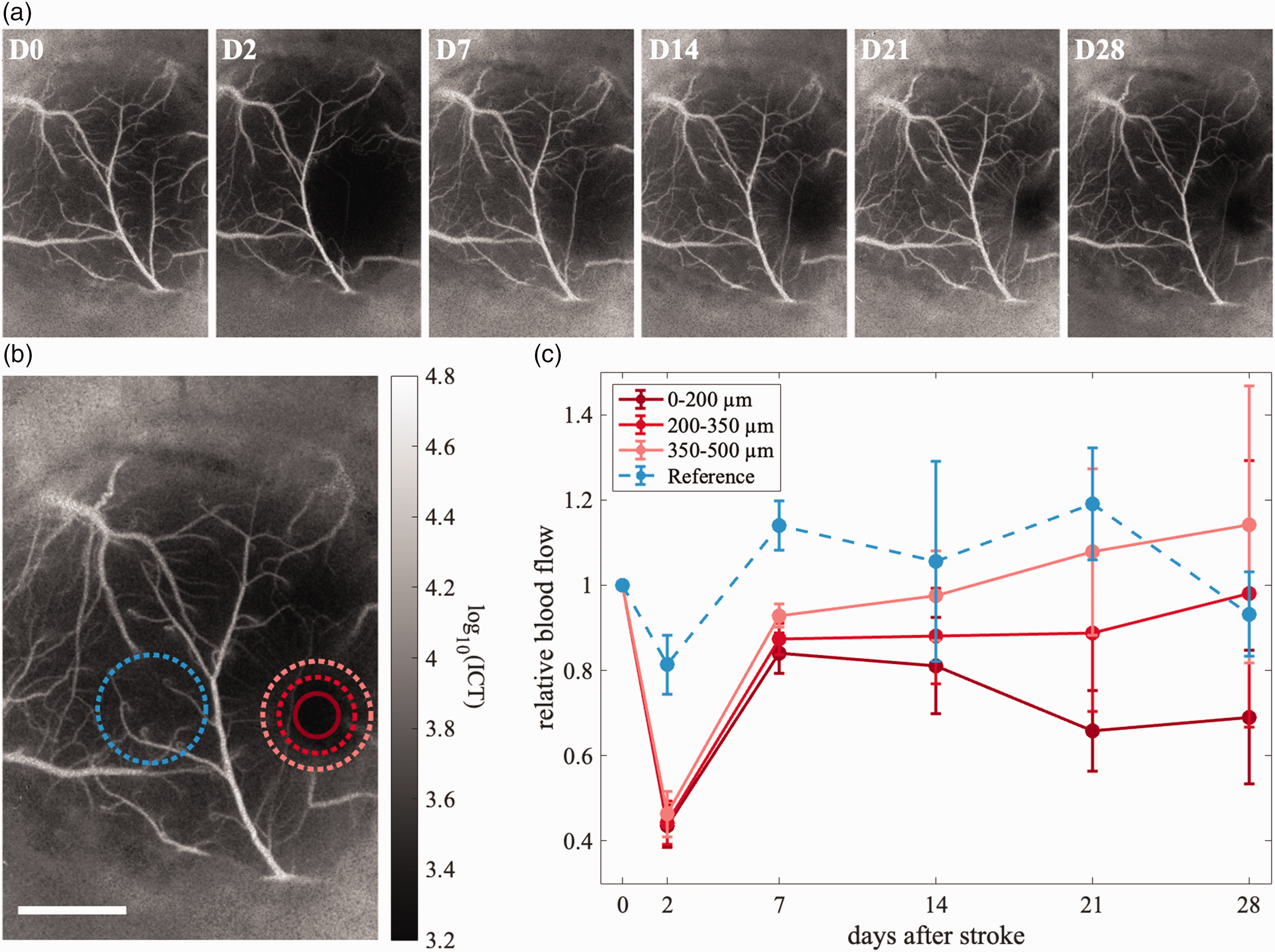
Blood flow following ischemia as determined from MESI: (a) ICT maps determined from MESI at each time point for one mouse. The day zero image was acquired immediately before photothrombosis, all others are labeled with the day after photothrombosis. (b) Regions where blood flow was determined for one mouse. The regions indicated in shades of red are for the ischemic area, the region indicated by blue is for the reference region. This image is the same as that shown on the far right in part A, and images in A are shown with the same display range indicated by the colorbar in B and (c) plots of average relative blood flow with time. Blood flow for the region closest to the infarct is shown in the darkest shade of red, flows for regions further away are shown in lighter shades. Blood flow for the reference region is shown by the dashed blue line. Error bars represent standard error.

Vascular perturbation is observed and quantified through vectorization with directional analysis

To longitudinally track the changes in vascular structure, five 2PM image sets at one-week intervals from all three stroke model mice were acquired, vectorized, and analyzed. Figure 4 shows the vectorizations for both the pre-ischemic states along with the conditions four weeks after photothrombosis. Similar ROIs relative to the infarct location are displayed for each animal. The vectorized reconstructions with color-coded orientation with respect to spherical ROIs reveal a consistent photothrombotic event with some differences in the extent to which the surrounding tissue is affected.

Figure 4.

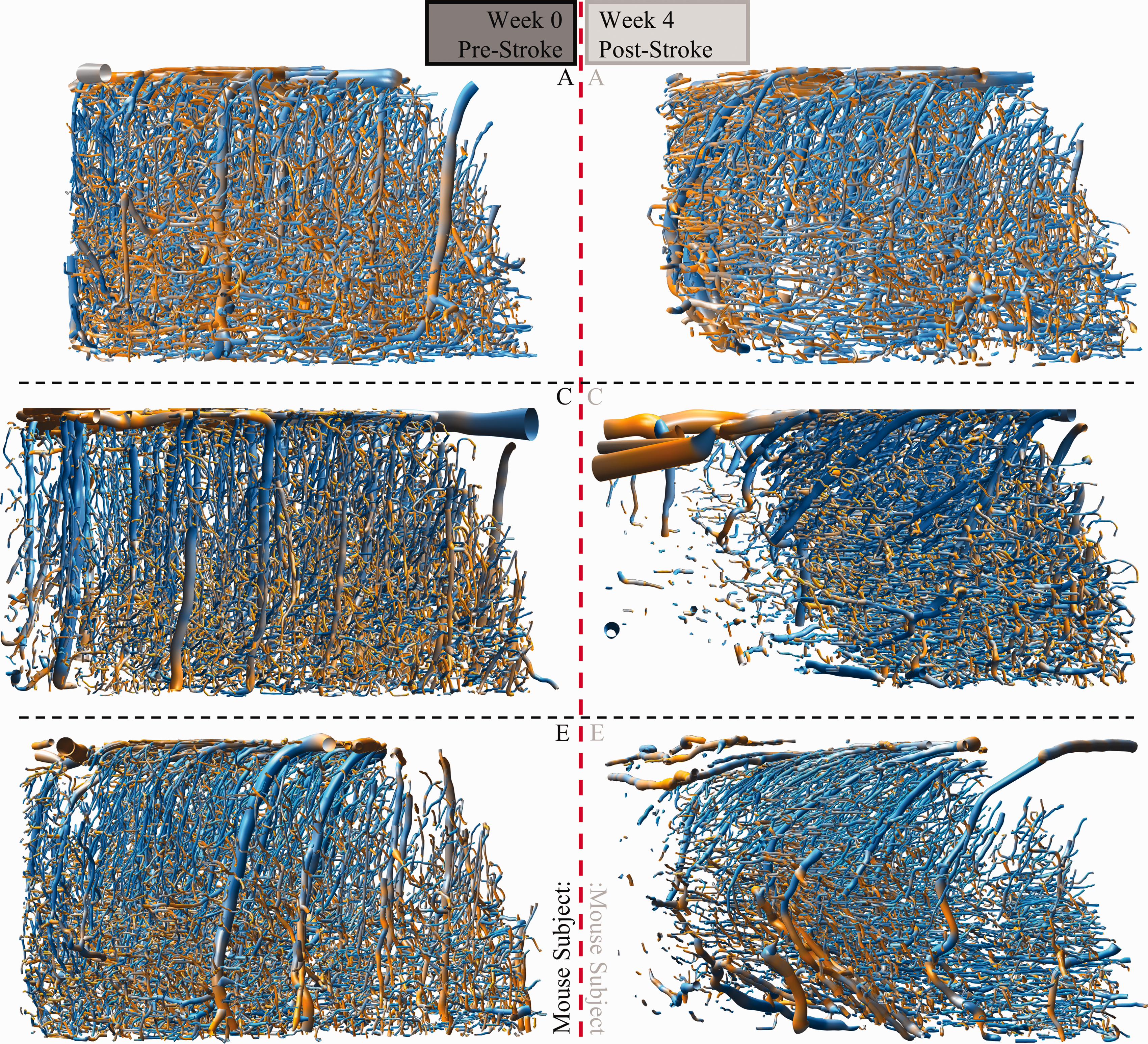
Pre- and Post-Stroke Snapshots by Subject: To compare the variation between stroke model subjects, week 0 pre- and week 4 post-stroke time points from three mouse subjects (A, C, and E) were imaged, vectorized, and analyzed. Similar spherical ROIs were selected between subjects, concentric with the infarct center observed at week 4. Vessels appear to be removed from or reoriented and pulled toward the infarct center to different degrees between subjects.

Figure 5 contains additional visualizations which show how the vascular network responds to photothrombosis in one animal. Vessels within about 500 μm from the infarct center have largely disappeared from the 2PM images one week after photothrombosis, likely due to lessened perfusion. Those in the surrounding 1 mm radius sphere appear to be pulled and reoriented toward the infarct from week 1 to week 4 post-stroke (Figure 5(a)). Figure 5(b) shows these same deformations in a three-dimensional reconstruction of the spherical ROI (∼1/2 mm³). For comparison, in Figure 5(c) similar ROIs for three time points in a healthy control animal are shown.

Figure 5.

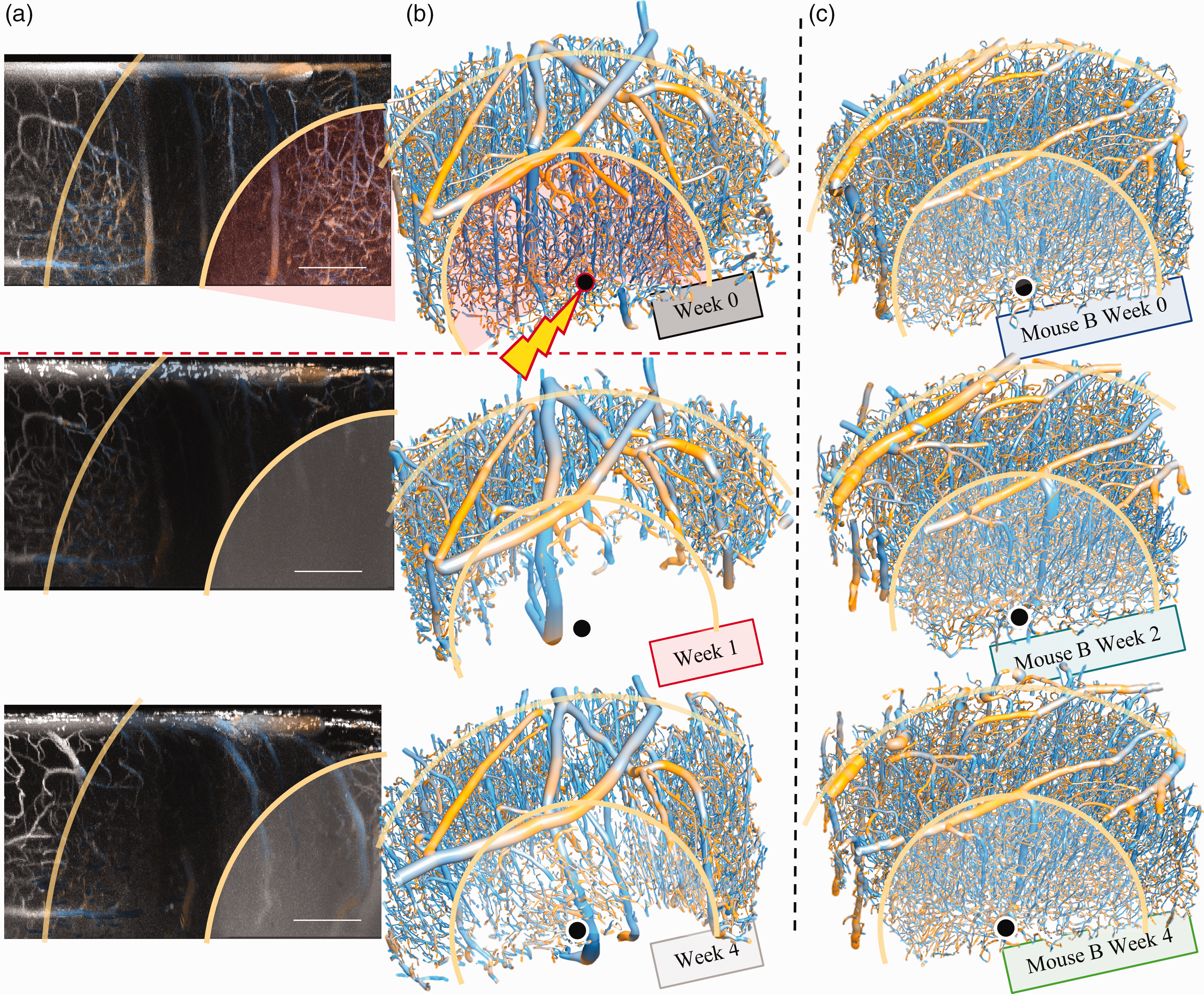
Longitudinal Stroke Model Snapshots: (a) Orthographic lateral MIPs of a rectangular volume (200 micron scale bar) of a raw 2PM image (concentric with the spherical ROI in the projection coordinate) for weeks 0, 1, and 4 post-photothrombosis. The orientation coloring for all vessel strands inside the (1 mm spherical) ROI overlays the original MIP. The tissue appears to contract toward the infarct center. (b) 3D perspective rendering of the strands within the ROI. A smaller (0.5 mm) ROI representing the core of the infarct is highlighted in red in week 0. Vessels in the core appear to be eliminated by the photothrombosis by week 1 and partially regrown by week 4 and (c) the time point renderings of the healthy control mouse B are shown for comparison.

Healthy vascular network is longitudinally stable with random statistical variations

In addition to providing rich visual information, directional analysis provides a means for quantitatively comparing the anatomy of two or more vascular networks. The unique statistical signatures of various metrics in both the healthy and ischemic vascular networks are presented in Figure 6 (distance and orientation by length), Figure S2 (strand length and tortuosity), Figure S3 (distance and orientation by strand), and Table 1. A total of twelve healthy time point snapshots from six subjects were analyzed to determine the healthy statistical signature and subject-subject variation (Table 1, “Healthy” row). Three of these are the baseline time points from the stroke models. Three control mice were imaged longitudinally to measure the baseline variation over three imaging sessions in healthy, adult subjects. A spherical ROI was selected in the control subjects to match the stroke model ROI shape and position with reference to the larger tiled image. Figure 6(a) shows the statistical signatures of distance and orientation with respect to the ROI center. The healthy control mice have longitudinally stable, reproducible vectorization statistics (Table 1) and three-dimensional reconstructions (Figure 5(c)).

Figure 6.

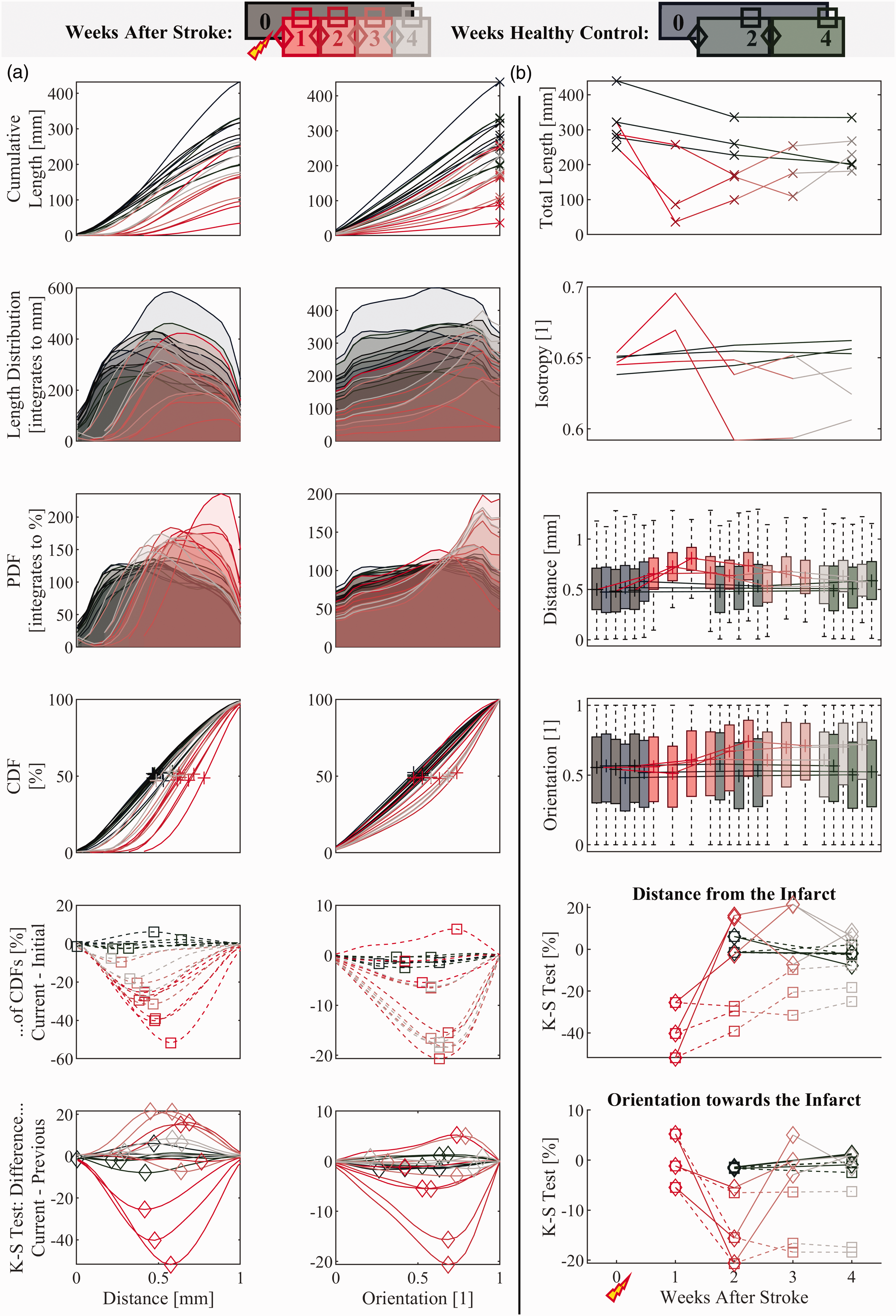
Longitudinal Stroke Model Statistical Analysis: The legend shows the color scheme given to the different snapshots (all mice have the same color at each time point). The healthy snapshots are darker colors, while the snapshots after photothrombosis begin red and fade to grey. The different marker symbols encode different comparisons (either vs. previous or vs. baseline). (a) Distribution snapshots of the length-weighted statistics for all time points healthy or stroke model vascular response to photothrombosis (From Top): cumulative length distributions of distance and orientation with respect to the ROI center, length-weighted Continued.histograms, normalized to PDF, integrated to CDF, and differences of CDFs between different pairs of time points. The K-S Test Statistics (extreme values of the differences of CDFs) summarize the differences between pairs of distributions. (b) Time courses of several statistics of interest (From Top): Total vascular length inside the ROI, overall isotropy, distance and orientation box and whisker plots (0,25,50 (median), 75,100th percentile), and K-S Test Statistics of the Distance and Orientation distributions (vs. the previous or the baseline).

Table 1.

Average signatures, subject variations, and statistical significances.

	Avg. Radius		Vol. Density		Area Dens.		Length Dens.		Strand Dens.		Junct. Dens.		Isotropy
	[µm]		[%]		[mm²/mm³]		[mm/mm³]		[1,000/mm³]		[1,000/mm³]		[1]
	by Length												by Length
	Avg.	St. D.	Avg.	St. D.	Avg.	St. D.	Avg.	St. D.	Avg.	St. D.	Avg.	St. D.	Avg.	St. D.
Healthy	3.6	0.4	2.3	0.6	8.9	2.4	390	120	6.5	1.7	2.9	1.1	0.84	0.01
Wk. 1	4.7	0.5	2.0	0.7	5.7	2.8	192	113	3.6	1.8	2.2	1.3	0.84	0.01
Wk. 2	3.9	0.0	1.5	0.4	5.5	1.4	226	55	4.7	0.8	1.3	0.2	0.85	0.01
Wk. 3	4.1	0.4	1.8	0.6	6.2	1.7	242	65	4.4	0.9	2.1	1.4	0.85	0.01
Wk. 4	4.0	0.2	2.1	0.3	7.3	0.5	293	20	5.1	0.4	2.8	1.5	0.85	0.01
	Diff.	Z-Sc.	Diff.	Z-Sc.	Diff.	Z-Sc.	Diff.	Z-Sc.	Diff.	Z-Sc.	Diff.	Z-Sc.	Diff.	Z-Sc.
	From the Healthy Condition
Wk. 1	1.1	1.7	−0.3	−0.3	−3.3	−0.9	−198	−1.2	−2.9	−1.2	−0.7	−0.4	−0.004	−0.3
Wk. 2	0.2	0.6	−0.7	−1.0	−3.4	−1.2	−165	−1.2	−1.8	−1.0	−1.6	−1.3	0.008	0.6
Wk. 3	0.4	0.7	−0.4	−0.5	−2.8	−0.9	−149	−1.1	−2.1	−1.1	−0.9	−0.5	0.010	0.8
Wk. 4	0.3	0.7	−0.2	−0.3	−1.6	−0.7	−97	−0.8	−1.4	−0.8	−0.2	−0.1	0.009	1.0
	From the Previous Condition
Wk. 1	1.1	1.7	−0.3	−0.3	−3.3	−0.9	−198	−1.2	−2.9	−1.2	−0.7	−0.4	−0.004	−0.3
Wk. 2	−0.8	−1.7	−0.4	−0.5	−0.2	−0.1	33	0.3	1.1	0.6	−0.8	−0.6	0.011	0.7
Wk. 3	0.2	0.4	0.3	0.4	0.7	0.3	16	0.2	−0.3	−0.2	0.7	0.5	0.003	0.2
Wk. 4	−0.1	−0.2	0.3	0.4	1.1	0.7	51	0.8	0.8	0.8	0.7	0.4	−0.001	−0.1
	K-S Test Statistic [1]												Isotropy[1]
	Distance		Orientation		Distance		Orientation		Length		Tortuosity
	by Length				by Strand
	Avg.	St. D.	Avg.	St. D.	Avg.	St. D.	Avg.	St. D.	Avg.	St. D.	Avg.	St. D.	Avg.	St. D.
Healthy		8%		4%		8%		3%		4%		4%	0.85	0.00
Wk. 1		10%		4%		10%		3%		6%		6%	0.85	0.01
Wk. 2		7%		6%		6%		5%		3%		3%	0.85	0.01
Wk. 3		10%		6%		10%		4%		5%		2%	0.86	0.01
Wk. 4		8%		6%		7%		5%		1%		2%	0.86	0.00
	Diff.	Z-Sc.	Diff.	Z-Sc.	Diff.	Z-Sc.	Diff.	Z-Sc.	Diff.	Z-Sc.	Diff.	Z-Sc.	Diff.	Z-Sc.
	From the Healthy Condition
Wk. 1	−25%	−2.0	−3%	−0.4	−26%	−2.0	−1%	−0.3	5%	0.7	5%	0.7	−0.004	−0.6
Wk. 2	−25%	−2.4	−14%	−1.9	−23%	−2.2	−12%	−2.1	10%	1.8	6%	1.3	0.005	0.7
Wk. 3	−12%	−1.0	−14%	−1.9	−12%	−1.0	−11%	−2.0	4%	0.6	7%	1.6	0.006	0.7
Wk. 4	−11%	−1.0	−15%	−2.1	−11%	−1.0	−12%	−1.9	2%	0.5	6%	1.3	0.007	1.4
	From the Previous Condition
Wk. 1	−25%	−2.0	−3%	−0.4	−26%	−2.0	−1%	−0.3	5%	0.7	5%	0.7	−0.004	−0.6
Wk. 2	3%	0.3	−13%	−1.7	7%	0.6	−11%	−2.1	5%	0.7	3%	0.4	0.009	1.1
Wk. 3	14%	1.2	1%	0.1	11%	1.0	2%	0.3	−6%	−1.0	1%	0.3	0.001	0.1
Wk. 4	3%	0.2	−1%	−0.1	2%	0.2	−1%	−0.2	−2%	−0.4	−2%	−0.9	0.001	0.1

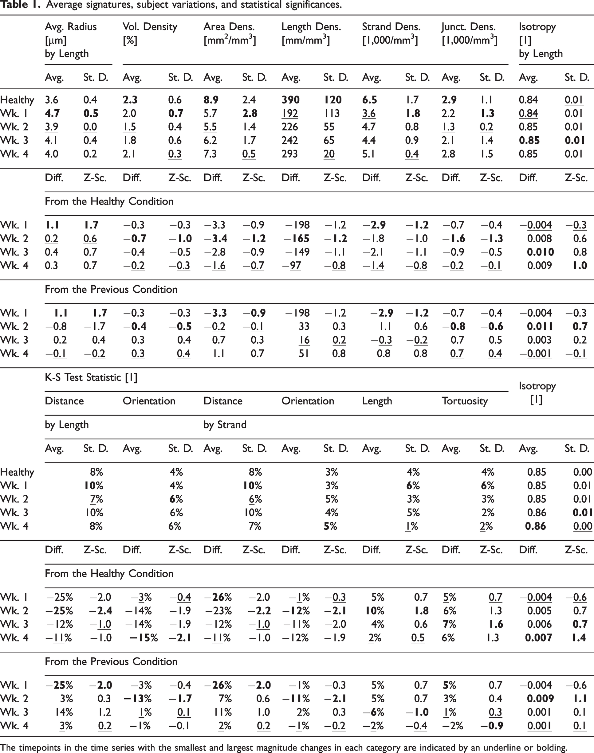
The timepoints in the time series with the smallest and largest magnitude changes in each category are indicated by an underline or bolding.

The statistical signatures are similar between all of the healthy snapshots, and the average and variation across subjects is shown in Table 1. Figures 6, S2, and S3 present histograms of many statistics of interest. To account for differences in sample size, each statistical distribution is normalized by total length to arrive at the probability distribution function (PDF), whose total area has a probability of 1 (100%). PDFs are integrated to cumulative distribution functions (CDFs) to compare their shapes across samples and to calculate the two-sample K-S test statistic, which can be conceptualized as the “distance” between statistical distributions in terms of probability (%). Longitudinal (finite) differencing of CDFs from healthy tissue shows random fluctuations in statistical distributions and represents a baseline in statistical variations (dark blue and green in Figures 6, S2, and S3), against which the stroke model is compared.

Vascular statistical signatures appear unique to pre-, intra-, and post-stroke conditions

Along with statistical distributions for the healthy control mice, Figure 6 also contains longitudinal distributions for 5 time points for the three ischemic mice. The total length of vessels (∼300 mm initially) and total number of strands (∼4,000 initially) were highly correlated through the ischemic recovery process (Figure 6(b) top and S2B top respectively). Both measured a large decrease at week 1 and then returned to the baseline by the week 4 time point.

The week 1 time point, which was acquired one week after photothrombosis, is significantly different from the baseline signature in terms of vessel distances from the infarct (Table 1, Figure 5(a)). In contrast, the normalized orientation signature is somewhat similar between weeks 0 and 1, however by week 4, it has trended significantly away from the baseline signature (by the K-S Test Statistic: Current - Initial) to a new steady state (Current - Previous). Meanwhile, the distance distribution smoothly returned to approximate the baseline signature by week 4. Therefore, there are unique, measurable characteristics to each of the pre-, intra-, and post-stroke conditions.

In addition to the length-weighted statistics (distance, orientation) which are defined for short vessel sections and have a large sample size, the strand-weighted statistics (distance, orientation, length, tortuosity) afford a greater number of network topological properties, however with a smaller sample size (Figure S3). The distance and orientation statistics of the strand objects closely match those of the section objects, although the binning/weighting is different. This result is unsurprising as an unbiased repartitioning of the vessel sections should yield a statistical distribution that is (unbiasedly, randomly) sampled from the original. The strand-length statistic distribution, shown in Figure S2B, shows a subtle but consistent dynamic peak (dotted line, square marker) at week 1. The strand-length gradually approaches the baseline. The strand-tortuosity statistic shows an even more subtle peak at week 1 (week 2 for one subject), followed by a gradual return to the baseline distribution.

Stroke model vasculature appears to reach a new stable signature after four weeks

To determine the baseline variances within which a new steady state could be determined, the distributions from the time-course stroke model mice (A, C, and E) and healthy control mice (B, D, and F) were compared (e.g. Figure 6(b), total length statistic and Figure 6(a), length-weighted distance and orientation statistics). The consecutive time CDF differences (solid lines, diamond markers, bottom of Figures 6(b), S2B, and S3B) show variations within the healthy control baseline for all statistics considered at four weeks post-stroke. Furthermore, the differences in the distance and orientation statistical distributions between the pre- and four weeks post-stroke time points were significantly (z-score, Table 1) larger than either the baseline inter-subject variations between the healthy pre- or between the four weeks post-stroke time points (dotted lines, square markers, bottom of Figures 6(b), S2B and S3B). Therefore, the vascular network reached a new steady state at four weeks after photothrombosis. The average radius (Table 1), and strand-length and -tortuosity (Figure S2B) statistics are relatively stable compared to the healthy control subjects (z-score, Table 1) and consistent with the in vivo healthy mouse cortex literature examples.^14,30 The box plots of Figures 6(b), S2B, and S3B show a more qualitative summary of the above statements.

Discussion

Advantages and disadvantages of the experimental tools

In this study, we employed LSCI, MESI, in vivo two-photon angiography, and vascular vectorization techniques to investigate the longitudinal stability of mouse cortical microvasculature and the effects of localized photothrombotic stroke. These experimental tools offer several advantages and disadvantages, which are important to consider when interpreting the results and designing future studies.

One of the major advantages of in vivo two-photon angiography is its ability to capture high-resolution images of the cortical microvascular networks. By imaging the same region at multiple time points, we can track the changes in the vascular network over time and investigate the dynamics of stroke recovery. Additionally, the use of MESI in combination with two-photon imaging provided a secondary means for monitoring vascular health following photothrombosis. We assume many vessels which disappeared from our two-photon images throughout the injury and recovery timeline did so due to alterations in perfusion and elimination. Through MESI, changes in perfusion were confirmed throughout this timeline to some degree. It is possible, however, that some vessels which became unresolvable during two-photon imaging did so because of an increase in background signal around the infarct rather than from drops in perfusion. We have no way of including these in our analysis, instead we normalized most of the statistical analysis by the sample size in some way (ROI volume, vessel length or number of strands) and took an ensemble statistical approach. Despite this limitation, we quantify and present views of clear structural changes in the vessels that could be resolved throughout the study.

Another advantage of our study is the application of vascular vectorization, specifically the Segmentation-less Automated Vascular Vectorization (SLAVV) software, which enabled the reconstruction and quantitative comparison of the vascular anatomy across samples. This automated method significantly reduced the manual burden of analyzing the large volumes of data obtained from the imaging sessions. Moreover, improvements made to the software, such as machine learning-assisted curation of the automated vector output and computational efficiency enhancements, contributed to the accuracy and efficiency of the vectorization process. The vectorization methods have potential use cases adjacent to the intended neuro-microvasculature use case: microvasculature in stroke,^46,47 eyes, ⁴⁸ ovaries, ⁴⁹ or in vitro.^50,51 Additionally, the vectorized output can be exported as a standard .ply or a special .vmv file for three-dimensional rendering and analysis using the vessmorphovis ⁵² plugin to blender (Blender Foundation, community).

The longitudinal design of our study, with weekly imaging sessions over one month, provided valuable insights into the stability and plasticity of the cortical microvascular networks. By comparing statistical distributions of the vectorized network longitudinally and between mice, we identified anatomical statistical signatures of healthy and stroke model vascular networks, as well as the dynamics of recovery. This longitudinal approach captured temporal changes that would have been missed in endpoint studies, providing a more comprehensive understanding of cerebrovascular plasticity.

Despite these advantages, there are also limitations associated with the experimental tools used in this study. First, in vivo two-photon angiography has restrictions in terms of the lateral field of view and imaging depth. Although we were able to cover large tissue volumes exceeding 1 cubic millimeter, the imaging range is still limited compared to the entire brain. This limitation may result in a partial representation of the vasculature and could introduce sampling biases.

Another limitation to the experimental method is in determining the underlying mechanism of the vascular response to stroke: Whether it is neuroplasticity, tissue deformation due to necrosis, or imaging quality artifacts remains unclear. The experimental tools used in this study provide valuable anatomical and statistical information, but they do not directly elucidate the underlying biological processes. Further investigations combining these tools with (ideally in vivo) molecular and cellular techniques could provide a more comprehensive understanding of the mechanisms driving vascular remodeling and recovery after stroke.

Length- vs strand-basis statistical analysis

The length-basis analysis focused on measuring the total vessel length and vessel length distributions within the vascular network. This approach provides insight into the overall structural changes in the vasculature. By comparing the length distributions between healthy and stroke-affected samples, we observed significant differences in distance and orientation, indicating vascular remodeling following stroke. Specifically, we observed a decrease in vessel length and reorientation of surrounding vessels toward the infarct in the stroke-affected samples compared to the healthy controls. This finding suggests a possible loss or pruning of vessel segments, followed by re-growth which is consistent with previous studies on post-stroke vascular remodeling. ⁵³

The strand-basis analysis, on the other hand, considered the individual vessel segments or strands within the network. By quantifying various parameters such as the number of strands and strand-length and -tortuosity, this analysis offers a more detailed understanding of the network's organization. We found that the stroke-affected mice exhibited significant decreases in the number of strands and junctions and changes to their strand-length, tortuosity and radius signatures compared to the healthy controls. These findings suggest a disruption in the vascular network connectivity and indicate a reorganization of the vascular architecture following stroke.

Microvascular anatomical statistical analysis interpreted

The results obtained from our study provide valuable insights into the acute microvascular changes associated with stroke, the remodeling processes, and potential implications for stroke recovery and rehabilitation. When interpreting the results, we can draw a correlation between our findings and the existing literature on vascular and neuronal plasticity in stroke models.

The pre-stroke condition is characterized by approximately uniform distributions of vessel length-density and orientation with reference to the (somewhat arbitrarily chosen in the case of the healthy subject) ROI center. The acute effects of the stroke are observed in the intra-stroke condition, with a significant drop in vessel length detected near the infarct center, importantly however the orientation signature is largely unchanged. The four-week post-stroke condition has approached a similar distance distribution to that of the pre-stroke condition. However, it has a different orientation signature which appears to be stable and unchanging by the end of the four weeks. These results are consistent with at least two possible explanations of neurovascular dynamics. One possibility is that the blood vessels are responding to the infarct by reorienting and growing towards the infarct. Another possibility is that the necrosed tissue is collapsing and pulling surrounding tissue toward the infarct center. This open question could possibly be answered by registering vectorized datasets and identifying and tracking vessels between time points.

The plasticity dynamics observed in this study are consistent with a previous study which employed manual capillary tracking. ¹⁶ The observed reorientation in the stroke-affected samples compared to healthy controls, suggests a restructuring of vessel segments following stroke. This finding is consistent with the concept of vascular remodeling, which involves structural modifications in response to ischemic events.^53,54 The reduced vessel length may reflect the retraction or elimination of vessel segments that are no longer necessary for the altered blood flow dynamics in the affected region. This remodeling process could be attributed to various factors, including reduced metabolic demands and changes in tissue perfusion patterns.

Moreover, the altered strand-length signature and decreased number of strands observed in the strand-basis analysis indicate a disruption in the network connectivity and organization following the stroke. Analysis suggests a restructuring favoring shorter, less tortuous strands. The vascular network is a highly interconnected system that ensures efficient blood supply to the brain, ⁵⁵ and the lasting alterations in network architecture observed in the orientation signature may contribute to the development of persistent functional deficits following stroke, as the changes to network connectivity could impair neurovascular coupling.

Understanding the biological implications of the observed vascular changes is crucial for devising effective stroke treatment and rehabilitation strategies.^56,57 The findings from our study highlight the need for targeted interventions that modulate vascular remodeling processes to promote optimal recovery after stroke. Therapeutic approaches that promote angiogenesis, vascular maturation, and network stabilization could potentially enhance blood flow restoration and support neuronal regeneration in the post-stroke period. ⁵⁸ Additionally, interventions aimed at enhancing collateral vessel growth and improving network connectivity may facilitate functional recovery by providing alternative routes for blood supply.

Furthermore, the insights gained from our statistical analyses can inform the development of computational models and simulations of the post-stroke vascular network response. ⁵⁹ These models can help investigate the complex interactions between vascular remodeling, tissue reorganization, and functional recovery. By integrating experimental data with computational models, we can gain a deeper understanding of the underlying mechanisms driving the observed vascular changes and their impact on stroke outcomes.

Results from our study on neurovascular plasticity after stroke correlate with existing literature on neuronal plasticity in stroke models^2,60 and hypoperfusion. ⁶¹ Similar to previous findings, we observed acute effects of a hypoxic injury after one week, with neurovascular rearrangement peaking at one or two weeks depending on the statistic considered. The neurovascular network reached a distinct stable state with a distinct orientation signature after four weeks. A correlation between neuronal and neurovascular plasticity is perhaps expected in consideration of the correlation between neuronal and microvascular densities. ²³

In conclusion, the results interpreted from our study shed light on the vascular alterations associated with stroke and provide a foundation for future investigations in stroke recovery and rehabilitation. The observed changes in network architecture offer valuable insights into the vascular remodeling processes following stroke. These findings have important implications for developing targeted interventions and computational models that aim to optimize stroke recovery and improve patient outcomes. Our results emphasize the dynamic nature of the neurovascular network after stroke.

Supplemental Material

sj-pdf-1-jcb-10.1177_0271678X241270465 - Supplemental material for Microvascular plasticity in mouse stroke model recovery: Anatomy statistics, dynamics measured by longitudinal in vivo two-photon angiography, network vectorization

Supplemental material, sj-pdf-1-jcb-10.1177_0271678X241270465 for Microvascular plasticity in mouse stroke model recovery: Anatomy statistics, dynamics measured by longitudinal in vivo two-photon angiography, network vectorization by Samuel A Mihelic, Shaun A Engelmann, Mahdi Sadr, Chakameh Z Jafari, Annie Zhou, Aaron L Woods, Michael R Williamson, Theresa A Jones and Andrew K Dunn in Journal of Cerebral Blood Flow & Metabolism