Sage Journals: Discover world-class research

Abstract

Executive Summary

Very large or complex data sets, which are difficult to process or analyse using traditional data handling techniques, are usually referred to as big data. The idea of big data is characterized by the three ‘v’s which are volume, velocity, and variety (Liu, McGree, Ge, & Xie, 2015) referring respectively to the volume of data, the velocity at which the data are processed and the wide varieties in which big data are available. Every single day, different sectors such as credit risk management, healthcare, media, retail, retail banking, climate prediction, DNA analysis and, sports generate petabytes of data (1 petabyte = 250 bytes). Even basic handling of big data, therefore, poses significant challenges, one of them being organizing the data in such a way that it can give better insights into analysing and decision-making. With the explosion of data in our life, it has become very important to use statistical tools to analyse them.

Keywords

Big Data Cluster Analysis Data Depth Non-parametric Inference Spatial Rank Function

Big data sets bring many challenges: They have huge volume and are growing rapidly. Thus, harnessing them for proper future usage is a difficult task.

Clustering is one of the most challenging aspects of big data analysis. Clustering is dividing data into some groups, which is often done without any or very little idea of previous knowledge about the data. One option of doing clustering might be looking at all possible groups of data which means sorting n observations into m groups. Even, for example, the number of possibilities of sorting 25 observations into 5 groups would be a very large number (Aldenderfer & Blashfield, 1984).

Clustering big data can be computationally expensive; hence, we need to use efficient methods of clustering. The clustering techniques also need to be robust as large data sets often contain outliers or extreme values. Unfortunately, most of the popular clustering techniques are not very robust. Using the idea of data depths, we propose a spatial ranking-based algorithm of clustering data, which is non-parametric, robust and is, therefore, better suited to handle big data.

In this article, we have discussed some existing clustering methods and then we go on to discuss spatial ranks and propose a rank-based clustering method. We also perform some simulations using our proposed method. Finally, we discuss the methodology adopted and extensions possible for this work.

SOME EXISTING CLUSTERING METHODS

Clustering is usually referred to as unsupervised learning (Ericson & Pallickara, 2013; Tibshirani, Walther, & Hastie, 2001). Usually, the grouping is done by using some measure of similarity or relationship: The basic concept is that within the groups, the objects should be as similar as possible to each other but between the groups, the observations should be as dissimilar as possible. In clustering, we try to focus on some patterns which can be found in the data and improve our learning based on that. Recognizing the pattern present in the data clustering helps us to split the data accordingly. Thus, according to the type of data, we also need to identify the best possible method of clustering.

The clustering algorithms can be divided, broadly, into two classes—hierarchical and non-hierarchical (Johnson & Wichern, 2015; Xu & Wunsch, 2005). The hierarchical algorithms attempt to build a tree-like nested structure, while the partitioning mechanisms divide the data into some predetermined number of, typically hard, partitions.

One of the main problems with any hierarchical clustering algorithm is that objects once classified cannot be reclassified at a later stage, and hence the final configuration of the clusters may not be sensible (Johnson & Wichern, 2015). These methods are not very robust towards outliers and become very slow for large data sets. This renders such methods unsuitable for analysis of big data.

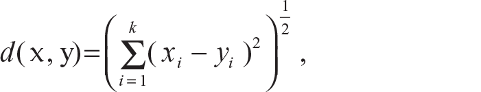
Another method of deciding on clusters is to use some similarity measure. There are many ways of deciding upon similarity or closeness between objects. Sometimes, distance functions are used to measure similarity. The distances can be measured in many different ways. Some of the popular distances between two k-dimensional data points are:

Euclidean distance (L₂ distance):

d (x, y) = {(Σ_{i = 1}^{k} {(x_{i} - y_{i})}^{2})}^{\frac{1}{2}},

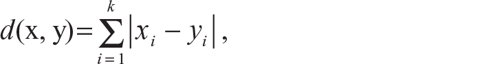
City block distance (L₁ distance):

d (x, y) = Σ_{i = 1}^{k} | x_{i} - y_{i} |,

Sup distance:

d (x, y) = \max_{1 \leq i \leq k} | x_{i} - y_{i} | .

Generalized Minkowski distance:

d (x, y) = {(Σ_{i = 1}^{k} {(x_{i} - y_{i})}^{m})}^{\frac{1}{m}},

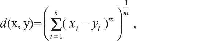
where for m = 1, we get the city block distance and for m = 2, we get the Euclidean distance.

The Mahalanobis distance which is also used for clustering of data is defined as follows:

d (x, y) = \sqrt{{(x - y)}^{T} Σ^{- 1} (x - y)},

where Σ is the within-group covariance matrix. If Σ is the identity matrix in the Mahalanobis distance, which means if the data points are not correlated, then we get the Euclidean distance between two data points.

More examples of distances are provided in Guha (2012), Johnson and Wichern (2015), and Xu and Wunsch (2005). Although it is good to use the actual distances for similarity measures which satisfy the distance properties (Johnson & Wichern, 2015), there might be situations where the observations cannot be represented by meaningful k-dimensional measurements. Then they have to be compared according to the presence or absence of a particular characteristic. If we denote presence by the value 1 and absence by the value 0, then it becomes a binary variable. Usually, a 1-1 match is gives a stronger measure of similarity than a 0-0 match. On these binary variables, the previously defined distance formula can be used to provide a measure of similarity but the problem is that these distance methods give equal weight to both 1-1 and 0-0 match cases which may not be desirable at all. Thus, to remove the effect of the 0-0 match, a frequency table of matches and mismatches is created. This table is very similar to a contingency table. Based on the frequency of the different types of matches and mismatches, some measures of similarities are developed. Some famous similarity coefficients for binary variables are matching coefficient (Sokal & Michener, 1958), Sneath and Sokal coefficient (Sneath & Sokal, 1973), and Gower and Legendre coefficient (Gower & Legendre, 1986). A categorical variable with two categories can be dealt with similarly as a binary variable, but if the variable has more than two categories, then it might not be a very helpful method. This problem arose during attempts with DNA sequencing. Jukes and Cantor (1969) suggested the logarithmic transformed genetic dissimilarity measure as

d_{A B} = - (\frac{3}{4}) I n [1 - (\frac{4}{3}) f_{A B}],

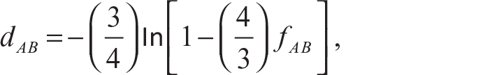
where f_AB is the dissimilarity between sequence A and sequence B. Tajima (1993) and Kimura (1980) suggested some modifications of this measure. Gower (1971) suggested a similarity measure which can be applied to mixed data type, namely continuous, ordinal or categorical variables, at the same time. Gower’s similarity coefficient S_ij compares two cases i and j and is defined as

S_{i j} = \frac{Σ_{k}^{n} w_{i j k} S_{i j k}}{Σ_{k}^{n} w_{i j k}},

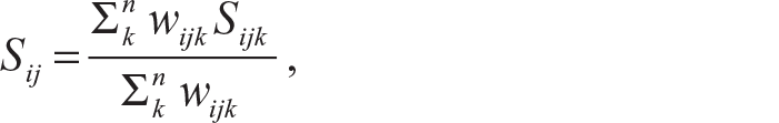
where S_ijk denotes the contribution by the kth variable and w_ijk is usually 1 or 0 depending if the comparison is valid for the kth variable. Karl Pearson’s correlation coefficient (Pearson, 1920) and Spearman’s rank correlation coefficient (Spearman, 1904) are some of the widely used similarity measurements.

The distance concept plays an important role in clustering as it not only helps to develop a similarity measure but also helps to develop a partitioning algorithm for clustering the data. The partitioning mechanisms to cluster data look at the distances among points of the data set.

The basic idea is to start with a pre-set number of clusters, say k, typically with some initial centres, then clustering the data into these k clusters to minimize the aggregate distances or a function thereof, re-assigning the centres, and iterating until convergence. Different distance measures are associated with different methods of clustering; for example, the ‘k-means clustering’ is associated with the Euclidean distance while the ‘k-median clustering’ is associated with the L₁ distance. The k-means method is one of the most popular and simple methods of clustering. The k-means algorithm was developed independently by different streams of science at the same time (Ball & Hall, 1965; Lloyd, 1982; Steinhaus, 1956). The name of this method was suggested by MacQueen (1967). This is a very simple, easy to implement, and efficient method of clustering and these are the main reasons for its popularity. As this method uses the Euclidean distance, it finds spherically shaped clusters. If the distance concept is changed to the Mahalanobis distance, then this method finds ellipsoidal clusters. Unfortunately, this method is sensitive to outliers. The basic concept of the k-means algorithm has been expanded in many ways. Some of those popular extensions are ISODATA (Ball & Hall, 1965), FORGY (Forgy, 1965), and fuzzy c-means (Dunn, 1973). Jain (2010) has provided a journey of the k-means method for the last 50 years.

Another very popular method of clustering is the parametric method (Fraley & Raftery, 2002; McLachlan & McGriffin, 1994). In this method, each cluster is assumed to have a basic parametric distribution which is known as a component. A statistical model is fitted to the data by the expectation maximization (EM) algorithm. Then the posterior probability of each mixture component for a given data point is calculated. The component possessing the largest posterior probability is chosen for that point. The points related with the same component form one cluster.

Most of the clustering techniques described above, with the exception of k-median clustering, use estimates of the unknown population moment parameters—mean, variance, correlation, and so on—and this makes these methods sensitive to outliers and extreme values. Hence, from the robustness perspective, non-parametric clustering techniques may be preferable. The k-nearest neighbour (kNN) method is a clustering method which is based on the set of partition. Here, clustering of the data points is based on their neighbours, that is, looking at majority voting based on k (a pre-set constant) of the nearest neighbours based on some metric. The kth nearest neighbour rule is perhaps the simplest and most appealing non-parametric clustering procedure (Jarvis & Patrick, 1973). However, application of this method is inhibited by lack of knowledge about its properties, and by the fact that it may be misleading when the data have significant skew (Hall, Park, & Samworth, 2008).

A possible solution is to use the relative data depth or relative rank-based ideas. Such classifiers, which are also non-parametric in nature, classify an observation into the class with respect to which the observation has the maximum location depth (Ghosh & Chaudhuri, 2005). Location depths are measures of the outlyingness of a data point with respect to the data cloud, defined based on different distance measures already discussed above. These depths can be used to define clusters in the data. Vardi and Zhang (2000) and Serfling (2002) gave a notion of L1 depth which is based on Chaudhuri (1996) and Koltchinskii’s (1997) concept of spatial quantiles. Jörnsten, Vardi, and Zhang (2002) introduced a concept of clustering which is based on Vardi and Zhang’s (2000) modified Weiszfeld algorithm. Partitioning around medoids or PAM (Kaufman & Rousseeuw, 2009) is a relatively robust method of clustering. In PAM, the medians belong to the data cloud but this makes PAM vulnerable to the chances of getting affected by noisy, high-dimensional data. In their work, Jörnsten, Vardi, and Zhang (2002) proposed a variant of the k-median method based on data depth which improves upon PAM and is claimed to be less affected by such problems. Different types of neural networks can also be constructed for classification (Jain, Murty, & Flynn, 1999; Xu & Wunsch, 2005), but these generally require a set of known samples for training. In our method, the initial training set is not required.

A MULTIVARIATE-RANK-BASED CLUSTERING METHOD

The k-median is robust and quite easy to compute; it is obtained by looking at the medians of each single dimension. As marginal distributions do not characterize the joint distribution, the co-ordinate-wise median cannot characterize a general multivariate distribution.

Chaudhuri (1996) extended the definition of the univariate quantiles to higher dimensions by defining the uth quantile Q(u) of X belonging to R^d as any minimizer of the function

E {ϕ (u, X - θ) - ϕ (u, X)},

where ‖u‖ <1 and ϕ(u, t) = ‖t‖ + u^Tt and ‖ . ‖ is the usual Euclidean norm. Such multivariate quantiles are also known as geometric quantiles or spatial quantiles. Chakraborty (2001) generalized the definition of geometric quantiles for other l_p distances. The ideas of geometric quantiles, in particular geometric median, can easily be used in formulating an alternative robust mechanism of clustering that is free of the weaknesses of coordinate-wise median discussed earlier. Towards that, we next define multivariate sign function followed by multivariate rank.

Definition 1: For x in R^d, the multivariate sign function is defined as

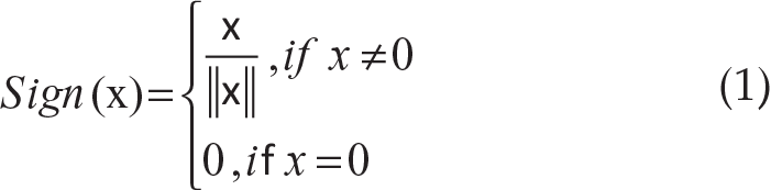
S i g n (x) = {\begin{cases} \frac{x}{‖ x ‖}, i f x \neq 0 \\ 0, i f x = 0 \end{cases}

(1)

where

‖ x ‖ = \sqrt{x_{1}^{2} + ... + x_{d}^{2},} x = {(x_{1}, ..., x_{d})}^{T} .

The sign function Sign(x) for x ≠ 0 gives the unit direction vector for x.

Definition 2: Suppose X in R^d is a random vector with distribution function F, which is absolutely continuous with respect to the Lebesgue measure on R^d. Then the multivariate spatial rank for a d-dimensional vector x with respect to X is defined as

R_{F} (x) = E_{F} (\frac{x - X}{‖ x - X ‖}) .

(2)

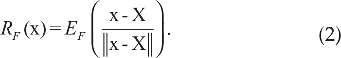
Note that the spatial median, θ, can be obtained by solving

R_{F} (θ) = 0

(3)

We can also see that the rank function R_F(x) is the inverse function of the multivariate geometric quantile function Q(u) defined by Chaudhuri (1996) in the sense that R_F(x) = u implies that Q(u) = x and vice versa. As the relation between data depth D(.) and the multivariate spatial rank R_F(.) would be given by D(x)= 1–‖R_F(x)‖, a measure of outlyingness can be defined using ‖R_F(x)‖. It can be verified that this outlyingness function is invariant under orthogonal and homogeneous scale transformations. For related discussion, one can see Serfling (2004, 2006). This rank orders the multivariate data in a central outward way. Smaller values of ‖R_F(x)‖ imply that x is located more centrally with respect to the data points and larger values of ‖R_F(x)‖ imply that x is an extreme point with respect to the data cloud. The direction of the vector R_F(x) suggests the direction in which x is extreme compared to the data cloud. Another important property of this rank function is ‖R_F(x)‖ < 1 for all x in R^d. For more properties of ‖R_F(x)‖, one can refer to Guha (2012).

We propose a rank-based clustering method based on multivariate rank defined in this section. Suppose X₁, X₂, …, X_n represent a data cloud in R^d, to be divided into k clusters. With respect to the data cloud, we can find the ranks of the observations x_is in that original cluster. Let it be denoted by R(x_i) for each x_i. For each cluster j, j = 1, …, k, we can find the ranks of the observation x_is in that particular cluster. We denote the within-cluster ranks by R^w_j(x_i) for x_is in that particular cluster j where j = 1, 2, … , k. Now, we look at the rank of the point x_i with respect to the other clusters. Let us denote it by R^o_j(x_i) for j=1, 2, … , k for j ≠ k.

The following is the algorithm for clustering:

Consider all the data points as one cluster and compute ‖R(x_i)‖ for each of the data points.

Fix k, the number of clusters. For simplicity let us suppose that k = 2.

Now we find the point x_Rmax which has the greatest ‖R(x_i)‖ value in the data cloud. We calculate the Euclidean distance of all the other data points from the point x_Rmax.

Now we look at the point x_Emax which is farthest from the point x_Rmax according to the Euclidean distance. Now calculate the Euclidean distance of all the points of the data cloud from the point x_Emax.

We initiate our clustering process with the help of the Euclidean distances of all the points of the data cloud, measured from the two points x_Rmax and x_Emax. We compare the two distances for each point. We put the point in cluster C1 if it is closer to the point x_Rmax. If the distance of the point in the data cloud is less with respect to the point x_Emax, then we put it into cluster C2.

Compute ‖R^w_j(x_i)‖ for each x_i in their respective clusters, where j = 1, 2.

Now take a point x_i from cluster C₁ and move it to cluster C₂ and calculate ‖R^o₂(x_i)‖. Then we compare ‖R^w₁(x_i)‖ and ‖R^o₂(x_i)‖. If ‖R^w₁(x_i)‖ < ‖R^o₂(x_i)‖, then we keep x_i in cluster C₁. If ‖R^w₁(x_i)‖ > ‖R^o₂(x_i)‖, then we move x_i to cluster C₂. We do this for each point x_i in cluster C₁.

We repeat the same operation for each element of cluster C₂.

Repeat steps (6)–(8) until convergence.

SIMULATIONS ON RANK-BASED CLUSTERING

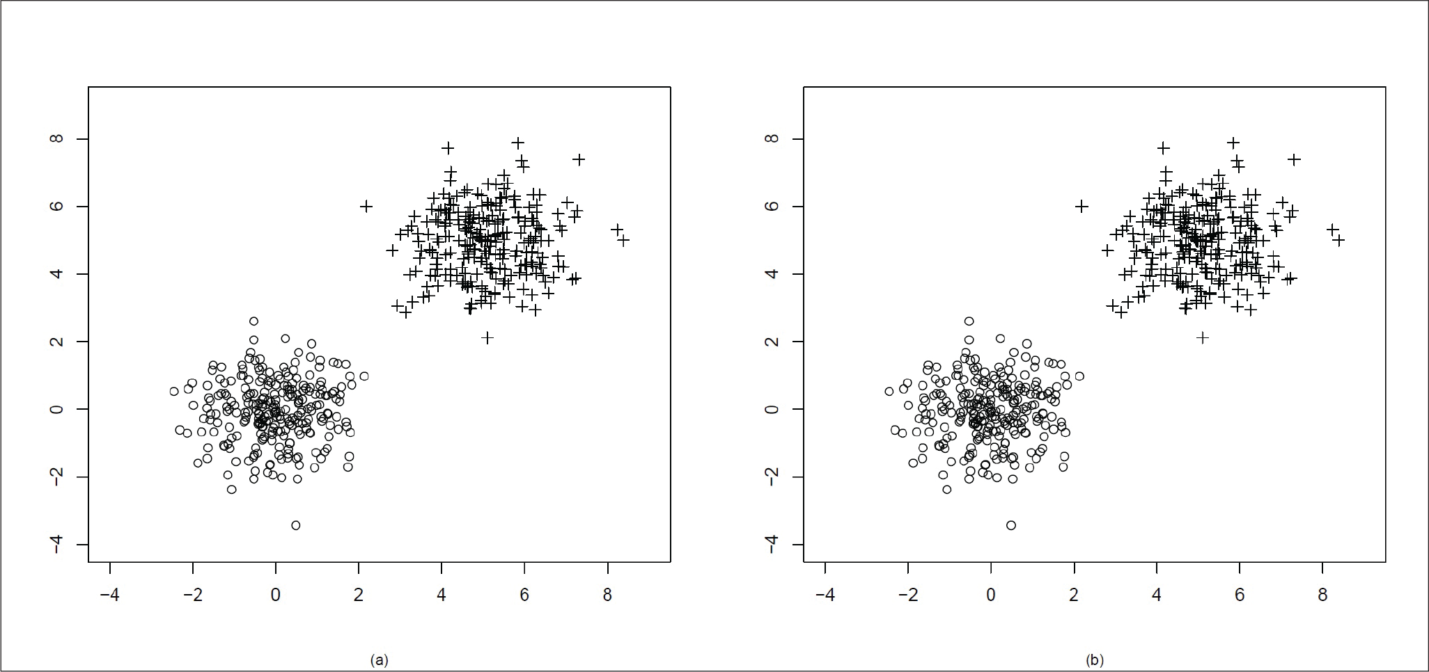
To illustrate our algorithm, we simulate some instances where the data come from two different distributions and hence are to be separated into two clusters. In each case, 500 data points are generated.

At first, we generate a mixture of data points from tean µ = (0, 0)^T, variance matrix $Σ$ = I₂, and bivariate normal distribution with mean µ = (5, 5)^T, variance matrix $Σ$ = I₂, where

I_{2} = (\begin{array}{l} 1 0 \\ 0 1 \end{array})

Both the distributions are spherical in nature.

In Figure 1(a), we can see the original clusters. In Figure 1(b), we see that the two clusters have been well separated by our algorithm.

In the next simulation, we take the data points from bivariate normal distribution with mean µ = (0, 0)^T, variance matrix $Σ$ = I₂ for one cluster. For the other cluster, we simulate the data points from bivariate normal distribution with mean µ = (5, 5)^T, variance matrix

Figure 1.

Mixture of Two Bivariate Normal Distributions µ = (0, 0)^T, Variance Matrix $Σ$ = I₂ and µ = (0, 0)^T, variance matrix $Σ$ = I₂

Figure 2.

Mixture of Two Bivariate Normal Distributions µ = (0, 0)^T, Variance Matrix $Σ$ = I₂ and µ = (0, 0)^T, variance matrix $\sum \begin{array}{l} (1) \\ 2 \end{array}$

Σ_{2}^{(1)} = (\begin{array}{l} 1 \\ 0.5 \end{array} \begin{array}{l} 0.5 \\ 1 \end{array}) .

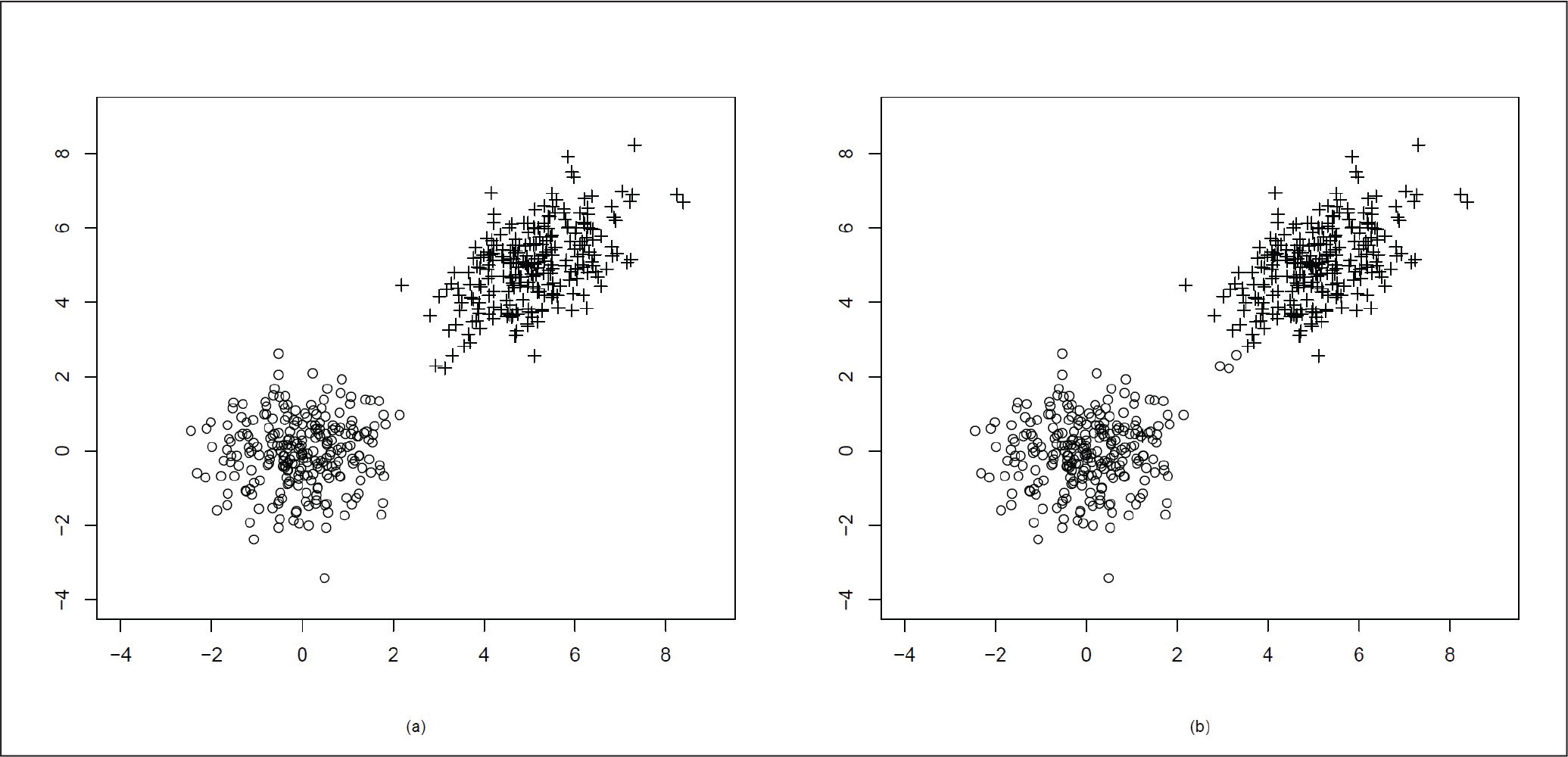
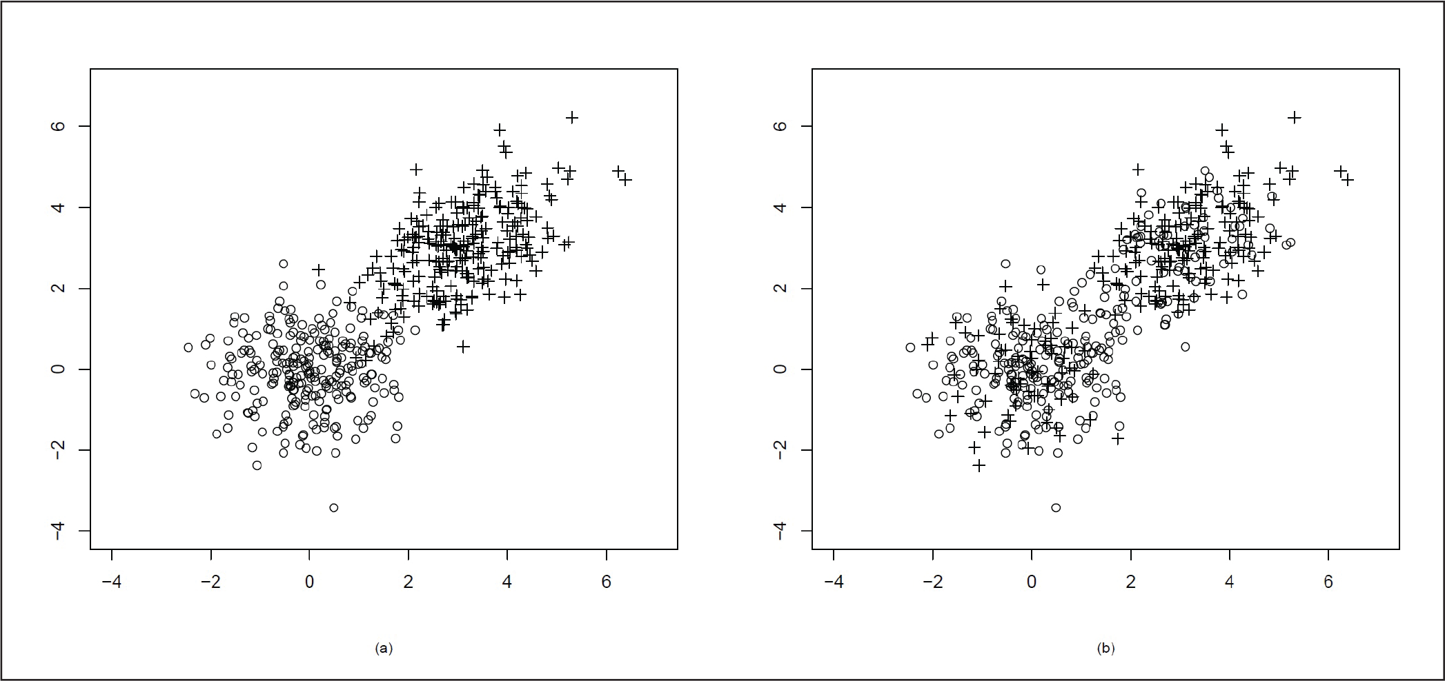
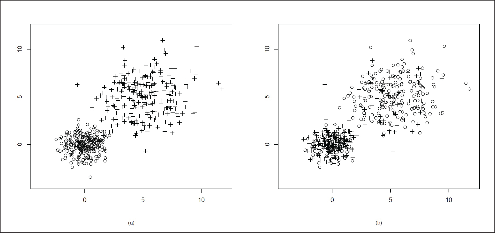
Here, as the correlation coefficient ρ = 0.5, the distribution is no longer spherical, but it becomes elliptical in nature. As the mean of the two clusters are µ = (0, 0)^T and µ = (5, 5)^T, the two clusters are quite far away from each other. We present the original data cluster in Figure 2(a) and the data after clustering using our proposed method in Figure 2(b). In Figure 2(b) we can see that the clusters are well divided with the exception of a few points.

In the next simulation, we move the two distributions a bit closer to each other. We generate the data points using bivariate normal distribution with mean µ = (0, 0)^T, variance matrix $Σ$ = I₂ and bivariate normal distribution with mean µ = (3, 3)^T, variance matrix $Σ$ = I₂. In Figure 3(a), we present the actual cluster. We can see from the figure that there is slight overlap between the two clusters. Figure 3(b) presents the data cloud after clustering using the rank-based method. In this case, the points which are well separated are in the correct clusters. In the overlap area, there are a very few misclassified points.

Figure 3.

Mixture of Two Bivariate Normal Distributions µ = (0, 0)^T, Variance Matrix $Σ$ = I₂ and µ = (3, 3)^T, variance matrix Σ = I₂

We generate the data points again from bivariate normal distribution with µ = (0, 0)^T, variance matrix $Σ$ = I₂ and bivariate normal distribution with µ = (3, 3)^T, variance matrix

Σ_{2}^{(2)} = (\begin{array}{l} 1 \\ 0.5 \end{array} \begin{array}{l} 0.5 \\ 1 \end{array}) .

Here, the two clusters are quite close to each other and there is an overlap. As ρ = 0.5 for the second cluster points, the distribution becomes elliptical.

Figure 4(a) presents the actual distribution of the data and Figure 4(b) shows the data clustering using our proposed method. In Figure 4(b), we can see that after clustering, some points at the far end of the other cluster have been misclassified. This might be due to the presence of the elliptical distribution in a very close neighbourhood of the spherical distribution.

Figure 4.

Mixture of Two Bivariate Normal Distributions µ = (0, 0)^T, Variance Matrix $Σ$ = I₂ and µ = (3, 3)^T, variance matrix $\sum \begin{array}{l} (2) \\ 2 \end{array}$ .

For the next case, we generate data points from a mixture of bivariate normal with µ = (0, 0)^T, $Σ$ = I₂ and µ = (5, 5)^T with $Σ$ = 4I₂. In this simulation, we are considering the two clusters well apart. In the second cluster, as the variance matrix is $Σ$ = I₂, though the data is spherical in nature, the spread of the data points is more than that in the initially considered cases. Figure 5(a) shows the actual data set and Figure 5(b) shows the clusters formed by our algorithm. In Figure 5(b), we can see that the clusters are not being well separated.

Figure 5.

Mixture of Two Bivariate Normal Distributions µ = (0, 0)^T, Variance Matrix $Σ$ = I₂ and µ = (5, 5)^T, variance matrix $\sum \frac{4}{2}$

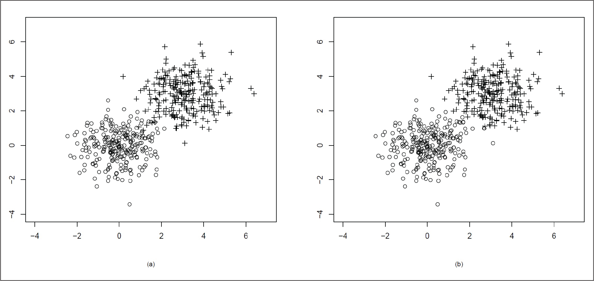
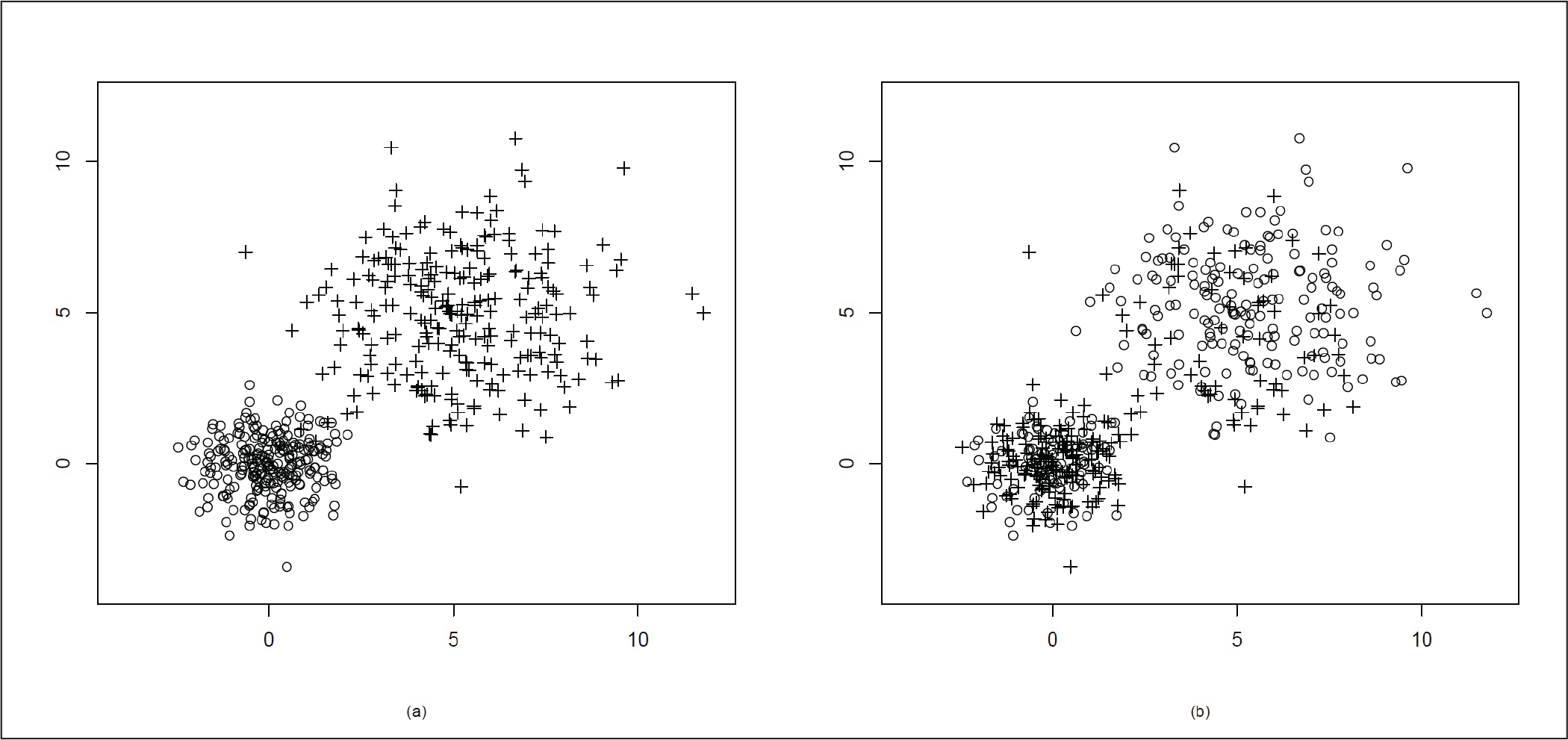
In the last set of simulation, we simulate two sets of bivariate normal data as before with one set being bivariate normal with µ = (0, 0)^T, variance matrix $Σ$ = I₂ and the other set being bivariate normal with µ = (5, 5)^T, variance matrix

Σ_{2}^{(3)} = (\begin{array}{l} 4 \\ 0.5 \end{array} \begin{array}{l} 0.5 \\ 4 \end{array}) .

The second cluster has more spread and is elliptical as ρ = 0.5. In Figure 6(a), we plot the actual data and in Figure 6(b), we plot the points according to the two clusters. In Figure 6(b), we can see that there is an overlap after clustering.

Figure 6.

Mixture of Two Bivariate Normal Distributions µ = (0, 0)^T, Variance Matrix $Σ$ = I₂ and µ = (5, 5)^T, variance matrix $\sum \begin{array}{l} (3) \\ 2 \end{array}$

AN APPLICATION OF THE TECHNIQUE

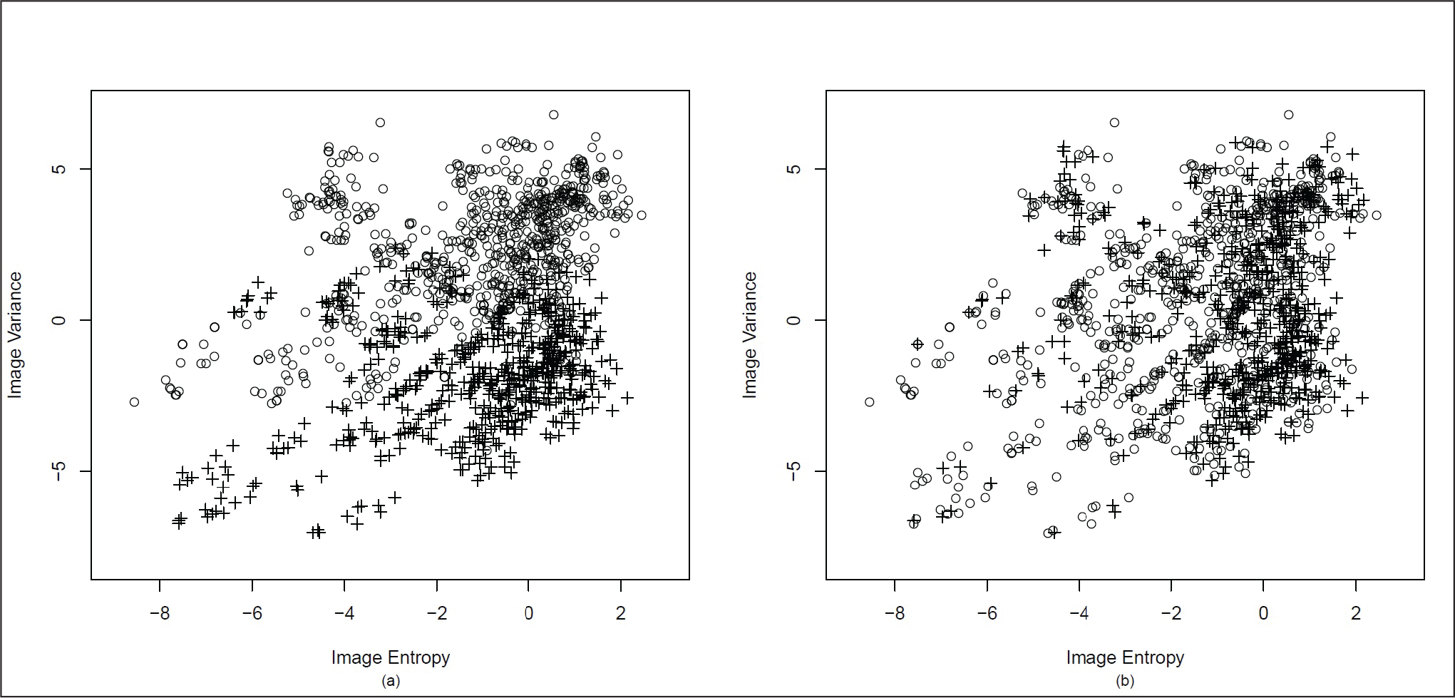
The banknote data has been used to apply the proposed method of clustering to a real data set. This data set consists of data extracted from images of genuine and forged banknote specimens.¹

https://archive.ics.uci.edu/ml/datasets/banknote+authentication (accessed on 28 September 2018).

Images of the banknotes were taken and wavelet transformation was used to extract the features of the images. The data set consists of 1,372 data points and 5 attributes (namely, variance, skewness, kurtosis, and entropy). In the data set, the fifth attribute gives us the true label for whether or not the banknote is genuine. If it is genuine, the label is 1 and otherwise it is 0. Using our clustering technique, we have tried to separate out the real bank notes from the fake ones. We have chosen the attributes entropy and variance to perform the clustering. Figure 7(a) represents the original grouping and Figure 7(b) represents the clustering obtained by the proposed method. From Figure 7(a), we can see that there is a huge amount of overlap in the data set. Our clustering technique has been able to identify and separate out some of the points.

Figure 7.

Bank Note Data (a) Original Clustering (b) Clustering Using the Proposed Method

DISCUSSION AND FUTURE WORK

Analysing and visualizing multidimensional data is not an easy task. We cannot apply the tools or techniques of the one-dimensional data directly to multidimensional data. They need to be modified. As the data generated in any field of our daily usage are multivariate in nature and the quantity is huge, it becomes difficult to handle the situation. In the case of big data, the data generated is not only multivariate in nature but also huge in volume. Thus, for this type of data, it might not be justifiable to look at only their marginal distribution.

The proposed rank-based clustering method is not based on any marginal distribution. In that sense, it is truly multivariate in nature. While using the rank-based technique, we do not require any distributional assumption. As the method is non-parametric, it is not very affected by the outliers, which means the method is robust. Hence, this clustering method is more resistant to noise than parametric methods. We have also considered the affine equivariant version of the spatial rank defined in Chakraborty (2001). The affine equivariant version of rank works well with a large section of elliptically symmetric distributions. Although the simulations in the second section are based on bivariate normal distribution, we plan to extend these simulations to other elliptical distributions. We have done our simulations for d = 2, the extension to d > 2 is immediate. We plan to extend it to higher dimensions in the future. The process of simulations is not computationally intensive. Each of our simulations, which were coded in C took only a few seconds to run on a machine with i3 processor with 4GB RAM. The volume of data generated is very large; thus, its analysis required a very quick method of computation. As our method takes very less computation time, it might be suitable for analysing big data.

In our illustrations, for simplicity, we have used two clusters; it can easily be extended to more than two clusters by slightly tweaking the algorithm provided earlier.

In clustering big data, one of the biggest issues would be determining the necessary number of clusters as big data set might consist of a variety of data which are being generated very fast in a large volume. Some methods of finding the number of clusters of data are discussed. Rousseeuw (1987), and Kaufman and Rousseeuw (2009) suggested the silhouette statistic, which is used for estimating the number of clusters. This method also provides a visual tool for partitioning. In this method for the ith observation, we define

a(i) = average distance to other points of its own cluster

b(i) = average distance to point in the nearest cluster besides its own

Then silhouette statistic is defined as

s (i) = \frac{a (i) - b (i)}{\max {a (i), b (i)}}

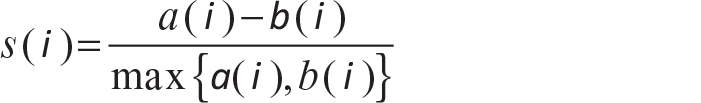
The value of s(i) lies between +1 and –1. With s(i) = +1, one can say that i has been well-clustered. The worst situation is when s(i) = –1, which means that i has been misclassified.

Tibshirani, Walther, and Hastie (2001) have proposed a method known as the gap statistic which estimates the number of clusters in a data set. It can be used with outputs obtained from k-means clustering as well as hierarchical clustering. Though gap statistic performs better than the silhouette method (Tibshirani, Walther, & Hastie, 2001), it often leads to over fitting (Jörnsten, Vardi, & Zhang, 2002). Jörnsten, Vardi, and Zhang (2002) have selected their number of clusters using relative L₁ depth, which is induced by the L₁ median. This relative data depth focuses on centrality and separation of data points, which makes it a good tool for determining the number of clusters. In future, we aim to develop a similar tool to determine the number of clusters using the rank method.

Declaration of Conflicting Interests

The author declared no potential conflicts of interest with respect to the research, authorship, and/or publication of this article.

Funding

The author received no financial support for the research, authorship, and/or publication of this article.

References

Aldenderfer

M. S.

Blashfield

R. K.

(1984). Cluster analysis . Thousand Oaks, CA: Sage Publications.

Ball

G. H.

Hall

D. J.

(1965). ISODATA: a novel method of data analysis and pattern classification . Menlo Park, CA: Stanford Research Institute International.

Chakraborty

(2001). ‘On affine equivariant multivariate quantiles.’ Annals of the Institute of Statistical Mathematics , 53(2), 380–403.

Chaudhuri

(1996). ‘On a geometric notion of quantiles for multivariate data.’ Journal of the American Statistical Association , 91(434), 862–872.

Dunn

J. C.

(1973). ‘A fuzzy relative of the ISODATA process and its use in detecting compact well-separated clusters.’ Journal of Cybernetics , 3(3), 32–57.

Ericson

Pallickara

(2013). On the performance of high dimensional data clustering and classification algorithms. Future Generation Computer Systems , 29(4), 1024–1034.

Forgy

E. W.

(1965). Cluster analysis of multivariate data: Efficiency versus interpretability of classifications. Biometrics , 21(3), 768–769.

Fraley

Raftery

A. E.

(2002). Model-based clustering, discriminant analysis, and density estimation. Journal of the American statistical Association , 97(458), 611–631.

Ghosh

A. K.

Chaudhuri

(2005). On maximum depth and related classifiers. Scandinavian Journal of Statistics , 32(2), 327–350.

10.

Gower

J. C.

(1971). A general coefficient of similarity and some of its properties. Biometrics , 27(4), 857–871.

11.

Gower

J. C.

Legendre

(1986). Metric and Euclidean properties of dissimilarity coefficients. Journal of classification , 3(1), 5–48.

12.

Guha

(2012). On scale-scale curves for multivariate data based on rank regions (Doctoral dissertation). Birmingham: University of Birmingham.

13.

Hall

Park

B. U.

Samworth

R. J.

(2008). Choice of neighbor order in nearest-neighbor classification. The Annals of Statistics, 36(5), 2135–2152.

14.

Jain

A. K.

(2010). Data clustering: 50 years beyond K-means. Pattern recognition letters , 31(8), 651–666.

15.

Jain

A. K.

Murty

M. N.

Flynn

P. J.

(1999). Data clustering: a review. ACM computing surveys (CSUR) , 31(3), 264–323.

16.

Jarvis

R. A.

Patrick

E. A.

(1973). Clustering using a similarity measure based on shared near neighbors. IEEE Transactions on computers , 100(11), 1025–1034.

17.

Johnson

Wichern

(2015). Applied multivariate statistical analysis . Chennai: Pearson Education India.

18.

Jörnsten

Vardi

Zhang

C. H.

(2002). A robust clustering method and visualization tool based on data depth. In Dodge

Yadolah

(Ed.), Statistical Data Analysis Based on the L1-norm and Related Methods (pp. 353–366). Basel: Birkhäuser.

19.

Jukes

T. H.

Cantor

C. R.

(1969). Evolution of protein molecules. Mammalian protein metabolism , 3(21), 132.

20.

Kaufman

Rousseeuw

P. J.

(2009). Finding groups in data: An introduction to cluster analysis (Vol. 344). Hoboken, NJ: John Wiley & Sons.

21.

Kimura

(1980). A simple method for estimating evolutionary rates of base substitutions through comparative studies of nucleotide sequences. Journal of molecular evolution , 16(2), 111–120.

22.

Koltchinskii

V. I.

(1997). M-estimation, convexity and quantiles. The annals of Statistics , 25(2), 435–477.

23.

Liu

McGree

Xie

(2015). Computational and statistical methods for analysing big data with applications . Cambridge, MA: Academic Press.

24.

Lloyd

(1982). Least squares quantization in PCM. IEEE transactions on information theory , 28(2), 129–137.

25.

MacQueen

(1967 June). Some methods for classification and analysis of multivariate observations. In Cam

Lucien M. Le

Neyman

Jerzy

(Eds.), Proceedings of the fifth Berkeley symposium on mathematical statistics and probability (Vol. 1, No. 14, pp. 281–297). Berkeley, CA: University of California Press.

26.

McLachlan

G. J.

McGiffin

D. C.

(1994). On the role of finite mixture models in survival analysis. Statistical methods in medical research , 3(3), 211–226.

27.

Pearson

(1920). Notes on the history of correlation. Biometrika , 13(1), 25–45.

28.

Rousseeuw

P. J.

(1987). Silhouettes: a graphical aid to the interpretation and validation of cluster analysis. Journal of computational and applied mathematics , 20(1), 53–65.

29.

Serfling

(2002). A depth function and a scale curve based on spatial quantiles. In Dodge

Yadolah

(Ed.), Statistical Data Analysis Based on the L1-Norm and Related Methods (pp. 25–38). Basel: Birkhäuser.

30.

Serfling

(2004). Nonparametric multivariate descriptive measures based on spatial quantiles. Journal of Statistical Planning and Inference , 123(2), 259–278.

31.

Serfling

(2006). Depth functions in nonparametric multivariate inference. In Liu

Regina Y.

Serfling

Robert

Souvaine

Diane L.

(Eds.), DIMACS Series in Discrete Mathematics and Theoretical Computer Science: Vol. 72, No. 1. Data depth: Robust multivariate analysis, computational geometry and applications . Providence, RI: American Mathematical Society.

32.

Sneath

Sokal

R. R.

(1973). Numerical Taxonomy; The Principles and Practice of Numerical Classification . San Francisco, CA: W. H. Freeman.

33.

Sokal

R. R.

Michener

C. D.

(1958). A statistical method for evaluating systematic relationships. Univ. Kansas Sci. Bull. , 38, 1409–1438.

34.

Spearman

(1904). The proof and measurement of association between two things. The American journal of psychology , 15(1), 72–101.

35.

Steinhaus

(1956). Sur la division des corp materiels en parties. Bulletin of the Polish Academy of Sciences , 1(804), 801.

36.

Tajima

(1993). Unbiased estimation of evolutionary distance between nucleotide sequences. Molecular biology and evolution , 10(3), 677–688.

37.

Tibshirani

Walther

Hastie

(2001). Estimating the number of clusters in a data set via the gap statistic. Journal of the Royal Statistical Society: Series B (Statistical Methodology) , 63(2), 411–423.

38.

Vardi

Zhang

C. H.

(2000). The multivariate L1-median and associated data depth. Proceedings of the National Academy of Sciences , 97(4), 1423–1426.

39.

Wunsch

(2005). Survey of clustering algorithms. IEEE Transactions on neural networks , 16(3), 645–678.

Application of Multivariate-Rank-Based Techniques in Clustering of Big Data

Abstract

Executive Summary

Keywords

SOME EXISTING CLUSTERING METHODS

A MULTIVARIATE-RANK-BASED CLUSTERING METHOD

SIMULATIONS ON RANK-BASED CLUSTERING

Mixture of Two Bivariate Normal Distributions µ = (0, 0)T, Variance Matrix Σ = I2 and µ = (0, 0)T, variance matrix Σ = I2

Mixture of Two Bivariate Normal Distributions µ = (0, 0)T, Variance Matrix Σ = I2 and µ = (0, 0)T, variance matrix ∑ (1) 2

Mixture of Two Bivariate Normal Distributions µ = (0, 0)T, Variance Matrix Σ = I2 and µ = (3, 3)T, variance matrix Σ = I2

Mixture of Two Bivariate Normal Distributions µ = (0, 0)T, Variance Matrix Σ = I2 and µ = (3, 3)T, variance matrix ∑ (2) 2 .

Mixture of Two Bivariate Normal Distributions µ = (0, 0)T, Variance Matrix Σ = I2 and µ = (5, 5)T, variance matrix ∑ 4 2

Mixture of Two Bivariate Normal Distributions µ = (0, 0)T, Variance Matrix Σ = I2 and µ = (5, 5)T, variance matrix ∑ (3) 2

AN APPLICATION OF THE TECHNIQUE

Bank Note Data (a) Original Clustering (b) Clustering Using the Proposed Method

DISCUSSION AND FUTURE WORK

Declaration of Conflicting Interests

Funding

References

Mixture of Two Bivariate Normal Distributions µ = (0, 0)^T, Variance Matrix $Σ$ = I₂ and µ = (0, 0)^T, variance matrix $Σ$ = I₂

Mixture of Two Bivariate Normal Distributions µ = (0, 0)^T, Variance Matrix $Σ$ = I₂ and µ = (0, 0)^T, variance matrix $\sum \begin{array}{l} (1) \\ 2 \end{array}$

Mixture of Two Bivariate Normal Distributions µ = (0, 0)^T, Variance Matrix $Σ$ = I₂ and µ = (3, 3)^T, variance matrix Σ = I₂

Mixture of Two Bivariate Normal Distributions µ = (0, 0)^T, Variance Matrix $Σ$ = I₂ and µ = (3, 3)^T, variance matrix $\sum \begin{array}{l} (2) \\ 2 \end{array}$ .

Mixture of Two Bivariate Normal Distributions µ = (0, 0)^T, Variance Matrix $Σ$ = I₂ and µ = (5, 5)^T, variance matrix $\sum \frac{4}{2}$

Mixture of Two Bivariate Normal Distributions µ = (0, 0)^T, Variance Matrix $Σ$ = I₂ and µ = (5, 5)^T, variance matrix $\sum \begin{array}{l} (3) \\ 2 \end{array}$