Sage Journals: Discover world-class research

Abstract

Executive Summary

Before financial liberalization, interest rates were administered and exhibited near-zero volatility. The easing of financial repression in the 1990s generated experiences with interest rate volatility in India. Administrative restrictions on interest rates in India have been steadily eased since 1993. This has led to increased interest rate risk for financial firms. Most research studies have almost exclusively focused on the developed countries especially the banking sector of the United States. The present study attempts to examine the interest rate risk of non-banking financial institutions in India by using the methodology of panel regression and generalized autoregressive conditional heteroscedasticity (GARCH) (1, 1) model for the period from 1 April 1996 to 30 August 2014. The sample used in the study consists of all non-banking financial companies (NBFCs) listed in the S&P CNX 500 index which has continuous availability of share prices over the study period. The study also examines the impact of unanticipated changes in interest rate on stock returns of NBFCs. The Box–Jenkins methodology is applied to calculate unanticipated changes in interest rate variable, autoregressive integrated moving average (ARIMA) (24, 1, 0) model. The time series used in the present study is found to be stationary at the first logarithmic difference. Stock returns exhibit significant exposure with both market returns and interest rate changes. The interest rate sensitivity of large, medium, and small financial institutions is also found to be different. Estimation results for the variance equation in GARCH (1, 1) model suggest that the volatility for individual firm stock returns is time-variant. The ARCH and GARCH coefficients are found to be significant, providing evidence against using traditional model (ordinary least square (OLS)) that assumes time-invariant volatility. This implies that the market has a memory longer than one period and volatility is more sensitive to its own lagged values than it is to new surprises in the market. This study also investigates the possible determinants that account for cross-sectional variation in the interest rate sensitivity of NBFCs. It is found that the size of the firm is the preferred determinant that accounts for cross-sectional variation in the interest rate sensitivity of finance companies. When unanticipated changes in interest rate are used in lieu of actual interest rate changes, not much difference is observed in the significance coefficients. The only significant difference observed is in the magnitude. The impact of actual interest rate changes is more than the impact of unanticipated interest rate changes in absolute terms. This difference in the magnitude of impact arises because actual data incorporate movement in both anticipated and unanticipated components of interest rate. Hence, NBFCs managers and regulators should adopt policies and strategies to avoid the transmission of interest rate risk in their stock returns.

Keywords

ARIMA Financial Sector GARCH Interest rate Panel Regression Stock Returns

In the pre-financial liberalization era, interest rates were administered and exhibited near-zero volatility. The easing of financial repression in the 1990s generated experience with interest rate volatility in India. Thereafter, administrative restrictions on interest rates in India have been steadily eased since 1993. This has led to increased interest rate risk for financial firms. Stock returns sensitivity to interest rates was theoretically advocated by Stone (1974). He developed the two-index model by incorporating the interest rate risk as an extra factor for explaining the stock returns of financial companies. Interest rate risk is an important concern for financial firms because the returns and costs of financial institutions are directly dependent on interest rates. Various authors have, therefore, examined the empirical sensitivity of stock returns of financial institutions to changes in market interest rates. Literature too shows a strong relation between the stock returns of financial institutions and interest rates. The bulk of the research has almost exclusively focused on the developed countries especially the banking sector in the United States. This study contributes to the related literature by studying the interest rate sensitivity of non-banking financial company’s (NBFC) stock returns in India.

OBJECTIVES OF THE STUDY

To examine whether stock returns of NBFCs in India exhibit significant sensitivity to interest rate changes.

To examine whether stock returns of NBFCs in India exhibit significant sensitivity to unanticipated changes in interest rate.

To examine whether interest rate sensitivity is uniform across financial institutions examined in the study.

To investigate possible determinants that account in favour of cross-sectional heterogeneity, if uniformity is rejected.

Data and Sources

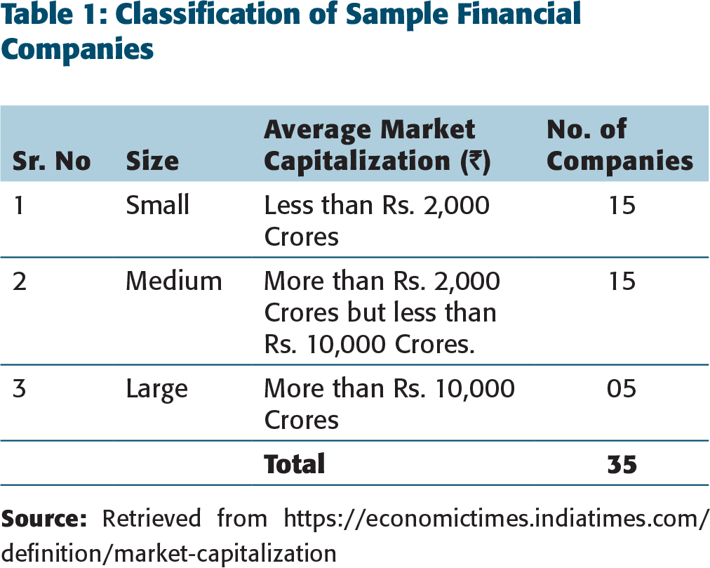
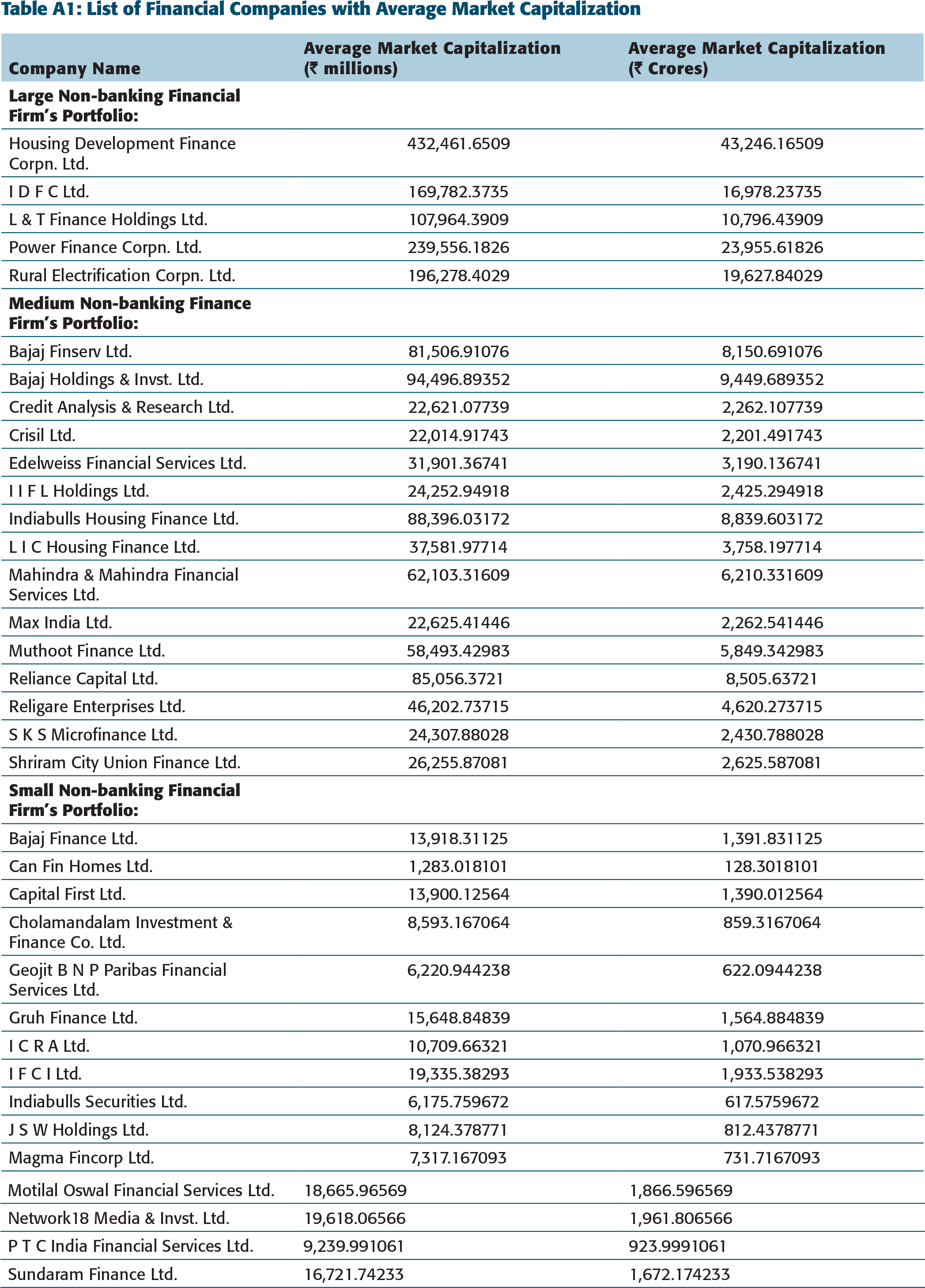
The sample used in the study consists of 35 NBFCs listed in S&P CNX 500 equity index that has continuous availability of share prices. The study period is from 1 April 1996 to 30 August 2014 covering approximately 18 years. Utilizing 35 stocks of non-banking financial firms, three portfolios are formed on the basis of average market capitalization—large, medium, and small in which each constituent stock is given an equal weight. Table 1 presents the classification of companies under sample on the basis of average market capitalization. The average market capitalization of the sample companies is presented in Table A1 of the Appendix.

Table 1:

Classification of Sample Financial Companies

Sr. No	Size	Average Market Capitalization (₹)	No. of Companies
1	Small	Less than Rs. 2,000 Crores	15
2	Medium	More than Rs. 2,000 Crores but less than Rs. 10,000 Crores.	15
3	Large	More than Rs. 10,000 Crores	05
		Total	35

Source: Retrieved from https://economictimes.indiatimes.com/definition/market-capitalization

The adjusted closing stock prices are collected on weekly basis. Thus, weekly data were used instead of daily data since sometimes market takes time to understand and reflect the effect of interest rate changes on stock prices. Weekly data also document weekly/intra-month variations in stock prices, which is not otherwise detectable in monthly data. Weekly stock returns of individual firms were used to create panel data work file. The panel data are a combination of time series and cross-sectional data. In the panel, data from a same set of cross-sectional firms are studied over time.

Weekly stock returns for individual firms were then used to create equally weighted portfolio returns for each group. This study analyses both the individual stock returns and portfolio stock returns because there is a trade-off between using portfolio data and individual firm data. When the individual firm data are used, there is a high noise in the data and results may be unduly influenced by the individual company multinational characteristics. On the other hand, the formation of portfolio returns has the advantage of smoothing out the noise in the individual data due to transitory shocks but it has the disadvantage of ignoring the dissimilarities in the individual firm characteristics. Therefore, this study investigates interest rate sensitivity of both portfolio stock returns and individual stock returns to accommodate these arguments. Finally, a set of financial variables from the firm’s balance sheets was used to investigate the determinants that account for cross-sectional variability in the interest rate sensitivity. It included working capital, leverage, size (measured by total assets of the firm), debt capital ratio, equity capital ratio, and loans.

Interest Rate Proxy

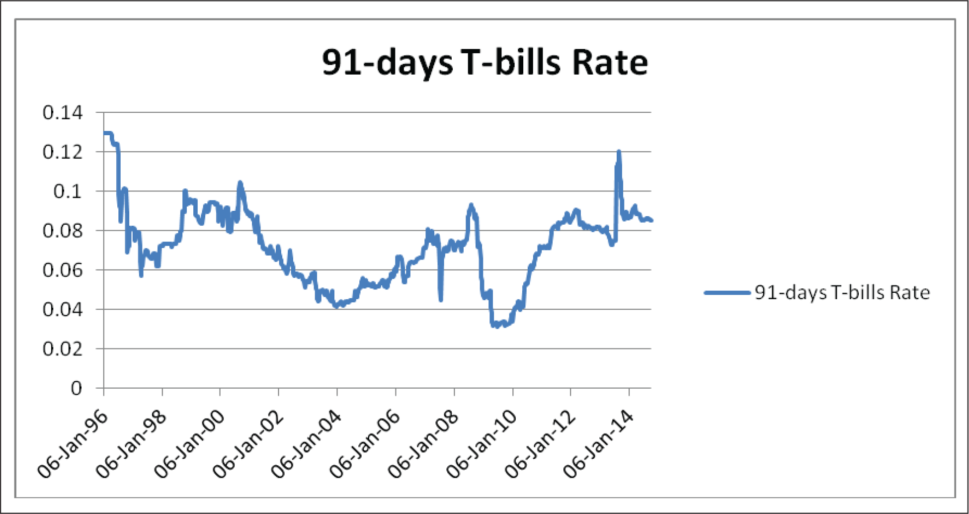
The cut-off implicit yield on 91-days treasury bills (T-bills) was used as the interest rate variable. This is because deregulated interest is determined by the forces of demand and supply in India. It is important to mention here that prior to 1993, the rate of return on 91-days T-bills was exogenously fixed at 4.60 per cent per annum. Administrative restrictions on interest rates have been steadily eased since 1993. It was only since January 1993 that a new auction-based system was introduced which allowed implicit yield on 91-days T-bills to vary. Data for cut-off implicit yield on 91-days T-bills have been collected from Reserve Bank of India (RBI) website.

Market Proxy

The return on the S&P CNX Nifty-500 equity index, the widest equity market index in India, is used as a proxy for market portfolio. It is a broad-based value-weighted market index generally used in research studies. The data regarding index values have been collected from the National Stock Exchange (NSE) website and Prowess database.

LITERATURE REVIEW

Stock returns sensitivity to interest rates was theoretically advocated by Stone (1974). He was the first one to develop the two-index model by incorporating the interest rate risk as an extra factor for explaining the stock returns of financial companies.

The stock returns interest rate sensitivity has long been the focus of academic research. Arbitrage pricing theory as developed by Ross (1976) argued that a number of systematic factors and not just market factor (captured by market risk premium) significantly explain stock returns. By employing factor analysis, study asserted that there are several systematic factors (industry specific and company specific) that affect the security’s return besides market returns such as unanticipated changes in interest rates, inflation rate, index of industrial production, trade deficit, etc. Since Stone (1974) developed the two-index model, Martin and Keown (1977), Lynge and Zumwalt (1980), Choi and Jen (1991) investigated whether inclusion of interest rate as an extra factor in the two-index model adds explanatory power for estimating stock returns (Latha, Gupta, & Ghosh, 2016).

Literature supports the Stone’s (1974) two-index model which attests the presence of interest rate as an extra market factor in explaining stock returns.

Dinesis and Staikouras (1998) examined the impact of interest rate changes (actual and unanticipated) on the common stock returns of portfolio of financial institutions in the UK. The autoregressive integrated moving average (ARIMA) model of Box–Jenkins methodology was used to calculate unanticipated interest rate movements. Results of the study suggested that actual and unanticipated interest rate changes both had a statistically significant negative effect on stock returns of financial as well as non-financial institutions in the UK but the impact was found to be lower for non-financial institutions. Financial institutions in the UK were seriously affected by the interest rate conditions and they had a significant exposure to interest rate.

Ballester, Ferrer, Gonzalez, and Soto (2009) investigated the determinants that account for cross-sectional variation in interest rate sensitivity across Spanish commercial banks. Most of the literature in the past has focused on the estimation of the relationship. The study found evidence for significant interest rate exposure in Spanish commercial banks. Interest rate sensitivity was found to be different for banks considered under study. Bank size and proportion of loans to total assets were found to be most important determinant accounting for interest rate risk heterogeneity across banks.

In the Indian context, interest rate risk was studied by Patnaik and Shah (2002) for a sample of 43 major banks. They found evidence for significant interest rate sensitivity of Indian banks. The two largest banks, SBI and ICICI bank, carried relatively little interest rate risk when compared to other banks in the sample. Size served as the hedging instrument for large banks. Hence, cross-sectional heterogeneity exists across banks for their interest rate exposure. Literature provided substantial evidence for stock returns exhibiting statistically significant inverse relationship with interest rate changes (Alam & Salahuddin, 2009; Asprem, 1989; Ballester, Ferrer, & Gonzalez, 2011; Ballester et al., 2009; Benink & Wolff, 2000; Kasman, Vardar, & Gokce, 2011; Kwan, 1991; J. D. Moss & G. J. Moss, 2010; Park & Choi, 2011).

RESEARCH METHODOLOGY

For each company under study, the log returns were computed because log return series are stationary; as a result, these are free from unit root and can therefore be easily compared with each other. Market returns were computed similarly. For calculating market returns widest equity market index in India, S&P CNX 500 is used as benchmark.

The first preliminary step in the analysis of time series data is the test of stationarity. Time series employed in the study should be free from unit root, that is, mean and variance of the time series should be constant overtime. This study consists of two data sets: individual time series and panel time series. Stationarity of individual time series and panel data series was tested using Augmented Dickey–Fuller (ADF test) and Levin, Lin, and Chu (LLC), (Levin, Lin, & Chu, 2002) test, respectively.

The financial time series are stationary at the first logarithmic difference.

Panel Regression Analysis

Panel data are a combination of time series and cross-sectional data. In panel data, the same set of cross-sectional firms was studied over time. The panel data have both space- and time-dimensional components of data. The panel data obtained are fitted to the equation by the regression method. The relationship between dependent and independent variables is determined and inferences are drawn on the basis of panel ordinary least square (OLS) regression analysis.

The following panel OLS model is employed to test the impact of market return and interest rate changes on stock returns:

R_{t} = α + β_{1} . R_{m} + β_{2} . Δ I_{t} + u_{t}

(1)

where R_t is the return of stock at time t; Rm is the return on the market index which is considered to reflect economy-wide factors; ΔI_t is the changes in interest rate; α is the intercept term; ut denotes the residual of the regression and represents that part of the returns that cannot be explained by market returns and changes in interest rate. The estimation of panel data regression can be done through two different approaches: fixed effect approach and random effect approach. The choice of approach between fixed effects approach and random effects can be made with the help of Hausman test (Bollerslev, Chou, & Kroner, 1992).

The observations made by Judge, Hill, Griffiths, Lutkepoul, and Lee (1982) may also be useful for making a choice between fixed and random effect model. According to them, if the time series data observations are large and cross-sectional units are small, there may be little difference in the value of the parameters estimated from fixed and random effects approach and fixed effect approach may be preferred.

GARCH (1, 1) Model

The generalized autoregressive conditional heteroscedasticity (GARCH) process, first introduced by Bollerslev, was estimated. In the Bollerslev GARCH model, the conditional variance is a linear function of past squared innovations and previous own lags. The GARCH (1, 1) process is specified as follows:

R_{t} = α + β_{1} . R_{m} + β_{2} . Δ I_{t} + u_{t}

(2)

σ^{2}_{t} = α_{0} + α_{1} u^{2}_{t - 1} + α_{2} σ^{2}_{t - 1}

(3)

where R_t is the return of stock at time t; α is the intercept term; R_m is the return on the market index, that is, S&P CNX 500 returns; ∆It is the change in interest rate; Δ_t² is the conditional variance since it is one-period ahead estimate for the variance calculated based on any past information about volatility; α₀ is the average volatility; α₁ is the previous period’s residual variance, the ARCH term and α₂ is the previous period’s forecast variance, the GARCH term. The GARCH specification requires that in the conditional variance equation, parameters α₀, α₁, andα₂ should be positive or non-negative. The sum of (α₁ +α₂) is a measure of volatility persistence, the closer to one, the higher the persistence in volatility. Therefore, in a conditional variance equation, the sum of α₁ and α₂ should be less than 1 to secure the covariance stationarity of the conditional variance. In case the sum is equal to 1, then the process is known as unit root in variance and the Integrated GARCH model (IGARCH) describes its behaviour. If α₁ + α₂ > 1, this would be termed as non-stationarity in variance.

For stationary GARCH models, conditional variance forecasts converge upon the long-term average value of the variance as the prediction horizon increases. For IGARCH processes, this convergence will not happen, while for α₁ + α₂ >₁, the conditional variance forecast will tend to infinity as the forecast horizon increases. (Brooks, 2002)

If the uniformity hypothesis is rejected, one would like to know the factors that account for cross-sectional variation in the interest rate sensitivity parameters (β₂’s). This study chose the only reliable and consistent balance sheet information available about the finance firms in the form of following financial variables: working capital, leverage, total assets, debt capital ratio, equity capital ratio, loans to total assets ratio.

Working capital (WC) = [Current Assets – Current Liabilities] working capital is used in logarithmic form to enable comparability of the estimated coefficients.

Leverage (LEV) = [Debt/ Equity].

Total assets (SIZE) = Firm size is frequently considered as the potential source of interest rate risk heterogeneity in the literature. In the present study, firm size (SIZE) is defined as the natural logarithm of total assets.

Debt capital ratio (DCR) = Debt capital ratio is the proportion of debt with respect to total assets of the firm. Firms with higher level of debt in their capital structure present higher level of interest burden, hence higher level of financial risk. For firms with high debt capital ratio, interest rate movements would have higher impact than those with low level of debt capital.

Equity capital ratio (ECR) = Equity capital ratio here is defined as the proportion of equity with respect to total assets of the firm. Firms with higher capital ratio presents lower needs of external funds, hence lower level of financial risk. For these firms, interest rate movements would have smaller impact on their costs and revenues and consequently, lower interest rate exposure (Ballester et al., 2009).

Loans to total asset ratio (LOANS) = Loans to total asset ratio is defined as the proportion of total loans with respect to total assets. Loans are an important determinant of interest rate sensitivity for financial firms as the interest income earned on the loans is a major source of revenue for financial firms.

The cross-sectional variation in the interest rate sensitivity of financial firms is analysed by using the following panel regression model:

β_{2 i} = γ_{i} + δ B S_{i} + u

(4)

where i = 1, 2…………n (across non-banking financial firms) and BS = (WC, LEV, SIZE, DCR, ECR, LOANS).

To generate the proxy for unexpected interest rate changes, this study uses the ARIMA model of Box–Jenkins methodology.¹

^***

The Box–Jenkins methodology refers to a set of procedures for identifying, fitting, and checking ARIMA models with time series data. Forecasts follow directly from the fitted equation model. ARIMA models do not involve independent variables in their construction. Instead, uses the information contained in the series itself to make forecasts. (Hanke & Wichern, 2009)

The initial selection of ARIMA model is based on examination of time series AC and PAC (p, q) for several time lags. After selecting the ARIMA model, it must be checked for adequacy. The model will adequate if residuals of the model are generally small, randomly distributed, and cannot be used to improve.

Table 2:

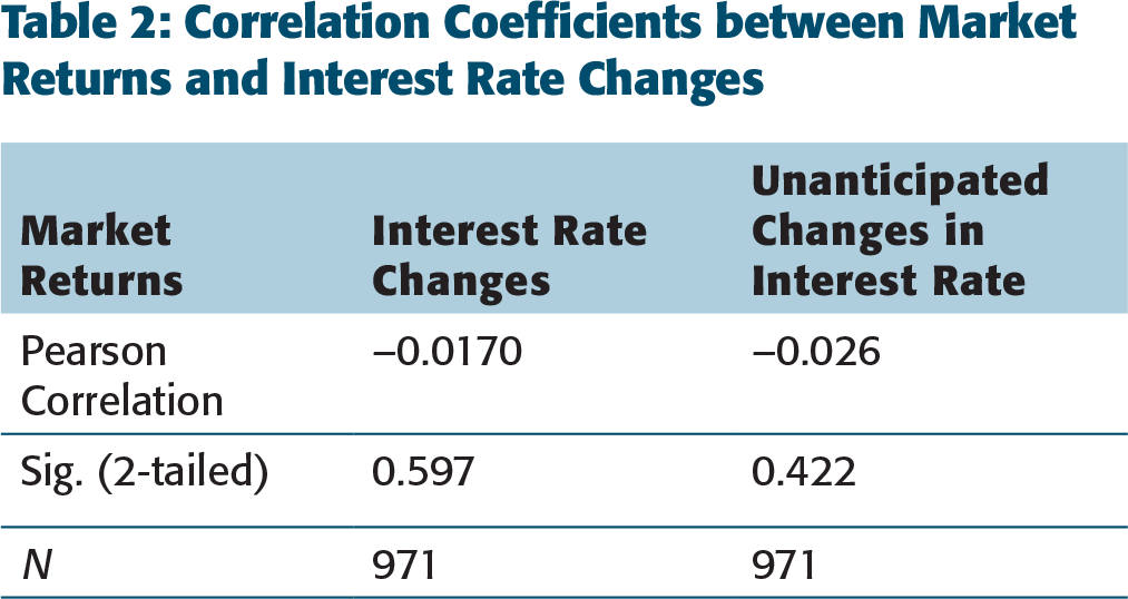
Correlation Coefficients between Market Returns and Interest Rate Changes

Market Returns	Interest Rate Changes	Unanticipated Changes in Interest Rate
Pearson Correlation	−0.0170	−0.026
Sig. (2-tailed)	0.597	0.422
N	971	971

EMPIRICAL RESULTS

The individual as well as panel time series used in the present study is non-stationary; however, it was found to be stationary at the first difference.

The correlation coefficients obtained between market returns and interest rate changes (actual and unanticipated) given in Table 2 are insignificant and do not present the problem of multicollinearity between the regressors.

Table 3 presents the results of the panel regression model using the random effect approach for the period ranging from 1 April 1996 to 30 August 2014. The estimates of Table 3 were calculated by using Equation (1) of panel regression analysis. The estimation of panel regression was done by using the simple OLS model. The panel regression analysis was used to estimate the effect of interest rate changes on NBFCs sector as whole.

Table 3:

Estimation of NBFCs Common Stock Returns with Least Square Random Effect Approach

CNX 500 Non-banking Companies	A	β₁	β₂	Adjusted R²	Hausman Chi-square Test Statistic
Stock Returns	0.0002(0.6337)	0.9964^*(0.0000)	−0.7476^*(0.0000)	0.2506	11.0306^*(0.0040)

Notes: $R_{t} = α + β_{1} . R_{m} + β_{2} . Δ I_{t} + u_{t}$

Values in parentheses indicate p-value.

^* indicates p-value significant at 1% level.

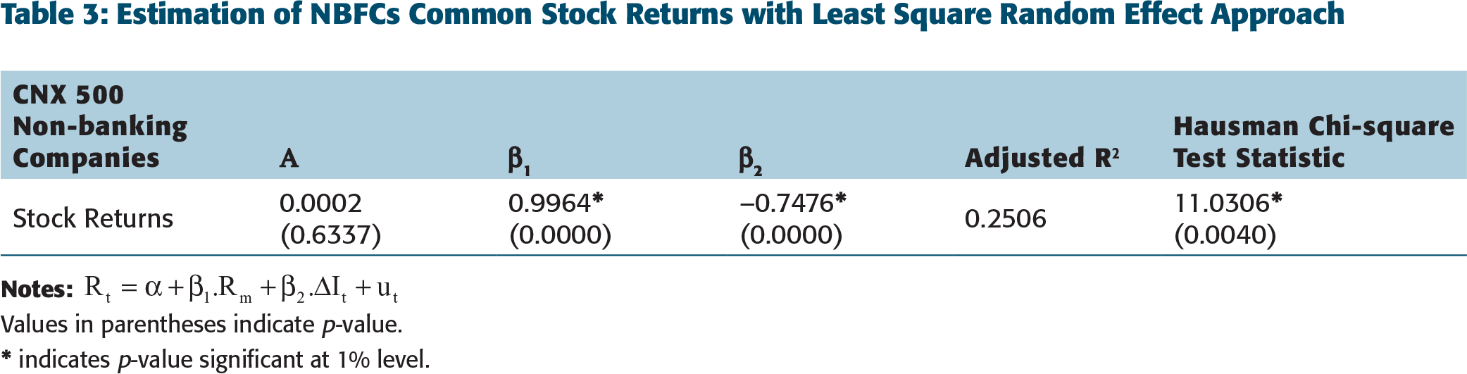
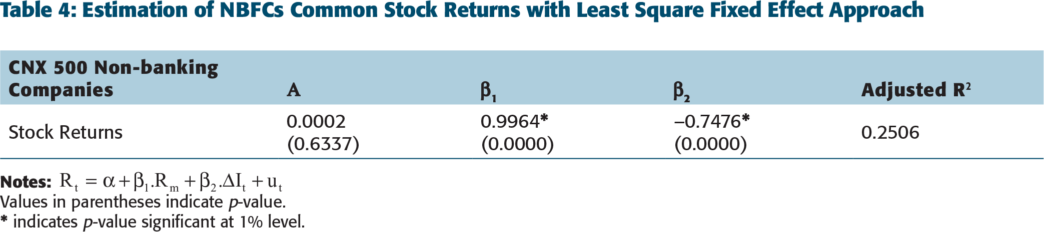
The results given in Table 3 suggest that β₁, the coefficient of market risk is positive and statistically significant for NBFC’s common stock returns. β₂, measuring the effect of interest rate changes on common stock returns, is negative and statistically significant, implying that the NBFCs in India are not protected from interest rate risk. The Hausman test is used for fixed versus random effects under the OLS regression model. The results of the Hausman test statistic are statistically significant at 1 per cent level, suggesting that the least square estimation requires the fixed effect approach for the reliable estimation of parameters (Hausman, 1978). Estimates of Table 4 were also calculated by using Equation (1).

Table 4 presents the effect of interest rate changes on common stock returns of NBFCs using the least square estimation fixed effect approach for panel analysis of data. The results obtained by using the least square fixed effect approach are similar to that obtained using the random effect approach ensuring accuracy of the estimated parameters from both the approaches of the panel regression model. It is observed from the results that the impact of market returns on non-banking financial firms conditional stock returns is larger than the impact of interest rate changes in absolute value implying that a major portion of their stock returns is explained by the market returns.

Table 4:

Estimation of NBFCs Common Stock Returns with Least Square Fixed Effect Approach

CNX 500 Non-banking Companies	A	β₁	β₂	Adjusted R²
Stock Returns	0.0002(0.6337)	0.9964^*(0.0000)	−0.7476^*(0.0000)	0.2506

Notes: $R_{t} = α + β_{1} . R_{m} + β_{2} . Δ I_{t} + u_{t}$

Values in parentheses indicate p-value.

^* indicates p-value significant at 1% level.

Thus, interest rate risk is significant for the NBFCs sector as a whole. However, this effect may or may not be uniform across all the firms studied. In order to assess the interest rate risk of each firm, we obtained sensitivity estimates by running separate regression for each firm employing GARCH (1,1) model.

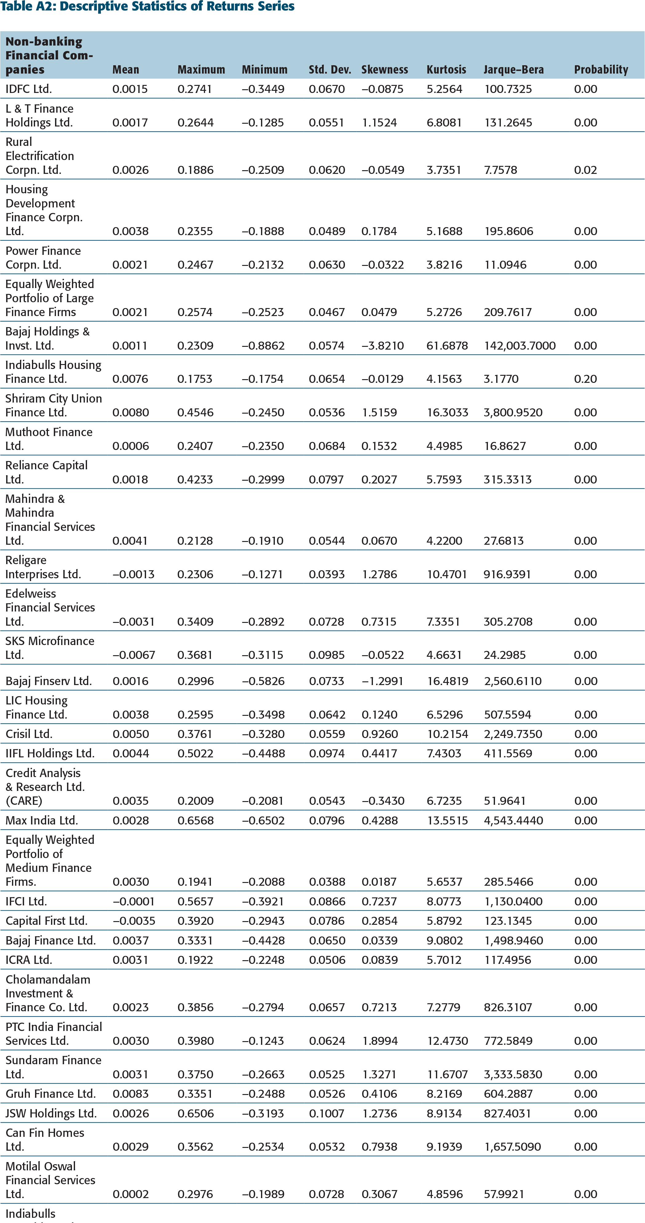
Financial time series data are often leptokurtic. They are also characterized by volatility clustering and leverage effects (Brooks, 2002). Therefore, financial time series violate the assumptions of the standard OLS model. Our data too have these features.²

It can be seen from Table A2 of the Appendix that data of each company are Leptokurtic. Figure 1 shows the volatility clustering in time series, that is, volatility occurs in bunches. Likewise, our data have leverage effect, that is, magnitude of change is more when prices fall as compared to when there is price rise.

Further, our financial time series in respect of individual companies as well as portfolio return series exhibits non-normality as evidenced by Jarque–Bera test (see Appendix, Table A2). Also, the value of Kurtosis is very high (>3) indicating the presence of extreme values in the returns distribution. Therefore obtaining the good fit requires adopting a conditional distribution with fatter tails (ARCH-GARCH type models) rather than normal distributions (Bollerslev et al., 1992). These features provide justification to employ GARCH (1, 1) model, that is, ARCH-type modelling technique. Therefore, it was decided to employ GARCH (1, 1) model, which takes care of these features of financial time series. The GARCH (1,1) model is more parsimonious and avoids overfitting. It contains only three parameters. It is less likely to breach the non-negativity constraints and allows infinite number of past squared error to influence current conditional variance. GARCH (1,1) model is sufficient to obtain a model fit for our data. Higher order model is not required because error terms are found to be significant at lag 1. Table 5 exhibits the estimation of NBFCs conditional stock returns with GARCH (1,1) model.

Table 5:

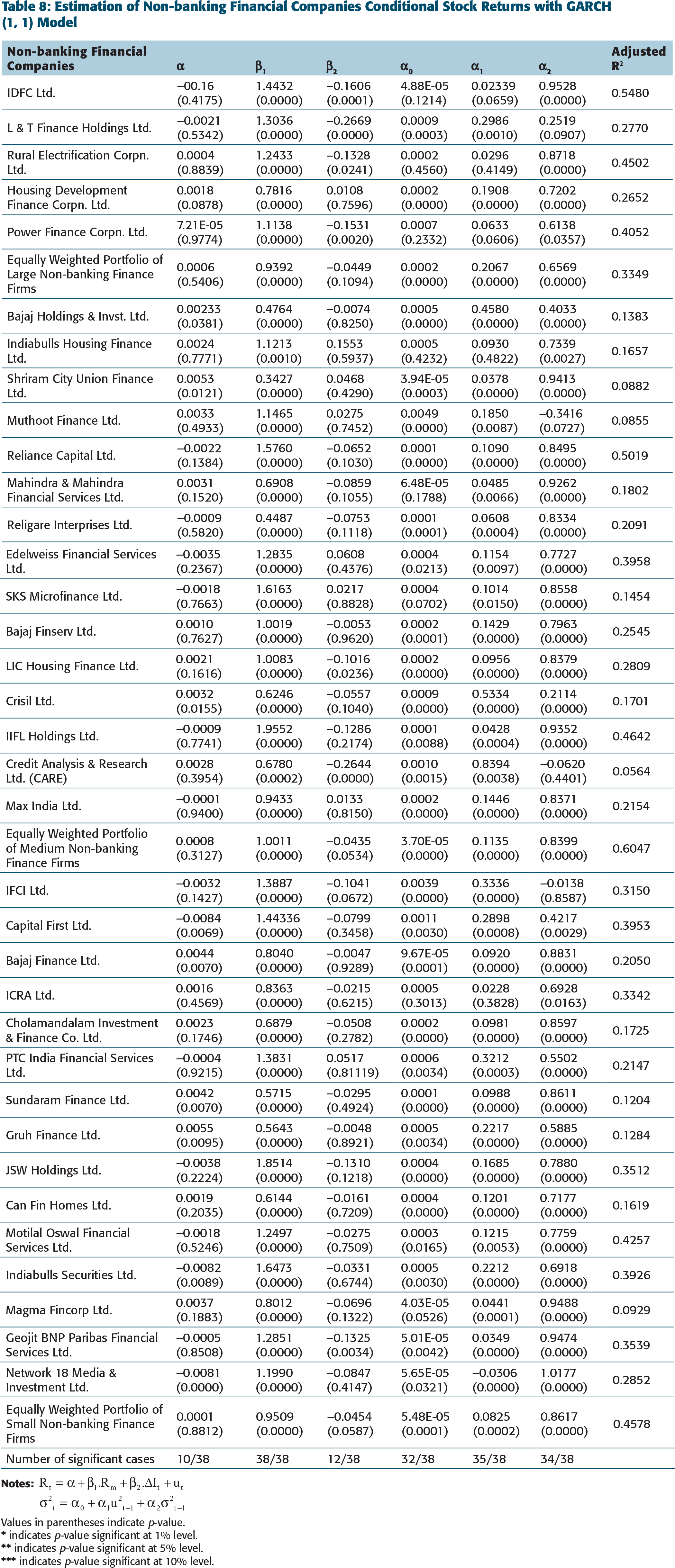
Estimation of Non-banking Financial Companies Conditional Stock Returns with GARCH (1, 1) Model

Non-banking Financial Companies	α	β₁	β₂	α₀	α₁	α₂	Adjusted R²
IDFC Ltd.	−0.0016(0.4183)	1.4430^*(0.0000)	−2.5007^*(0.0000)	4.69E-05(0.1640)	0.0243^***(0.0626)	0.9523^*(0.0000)	0.5458
L & T Finance Holdings Ltd.	0.0006(0.7935)	1.3650^*(0.0000)	−3.0843^*(0.0000)	0.0011^*(0.0000)	0.5797^*(0.0028)	−0.1075(0.1401)	0.2591
Rural Electrification Corpn. Ltd.	0.0004(0.8612)	1.2372^*(0.0000)	−2.4662^**(0.0193)	0.0002(0.4772)	0.0229(0.4773)	0.8903^*(0.0000)	0.4512
Housing Development Finance Corpn. Ltd.	0.0018^***(0.0885)	0.7812^*(0.0000)	0.0767(0.8800)	0.0002^*(0.0000)	0.1898^*(0.0000)	0.7215^*(0.0000)	0.2630
Power Finance Corpn. Ltd.	−9.97E-05(0.9685)	1.1126^*(0.0000)	−3.1384^*(0.0000)	0.0009(0.2694)	0.0638^***(0.0811)	0.5515(0.1373)	0.4086
Equally Weighted Portfolio of Large Finance Firms	0.0006(0.5667)	0.9380^*(0.0000)	−0.9500^**(0.0319)	0.0002^*(0.0000)	0.2079^*(0.0000)	0.6519^*(0.0000)	0.3364
Bajaj Holdings & Invst. Ltd.	0.0023^*(0.0377)	0.4770^*(0.0000)	0.0013(0.9976)	0.0006^*(0.0000)	0.4582^*(0.0000)	0.4034^*(0.0000)	0.1356
Indiabulls Housing Finance Ltd.	0.0023(0.7779)	1.1223^*(0.0000)	1.4478(0.6570)	0.0005(0.4457)	0.0926(0.4921)	0.7308^*(0.0065)	0.1103
Shriram City Union Finance Ltd.	0.0053^*(0.0123)	0.3418^*(0.0000)	0.4932(0.5734)	3.98E-05^*(0.0003)	0.0379^*(0.0000)	0.9409^*(0.0000)	0.0825
Muthoot Finance Ltd.	0.0030(0.5351)	1.1396^*(0.0000)	0.8306(0.3062)	0.0049^*(0.0000)	0.1795^*(0.0094)	−0.3549^***(0.0938)	0.0694
Reliance Capital Ltd.	−0.0022(0.1300)	1.5776^*(0.0000)	−0.5871(0.2417)	0.0001^*(0.0000)	0.1084^*(0.0000)	0.8496^*(0.0000)	0.4998
Mahindra & Mahindra Financial Services Ltd.	0.0031(0.1549)	0.6913^*(0.0000)	−0.7546(0.3037)	6.63E-05(0.1715)	0.0490^*(0.0069)	0.9253^*(0.0000)	0.1707
Religare Interprises Ltd.	−0.0010(0.5680)	0.4496^*(0.0000)	−0.6825(0.3237)	0.0001^*(0.0001)	0.0578^*(0.0004)	0.8365^*(0.0000)	0.2018
Edelweiss Financial Services Ltd.	−0.0035(0.2379)	1.2826^*(0.0000)	0.7628(0.4785)	0.0004^**(0.0208)	0.1154^*(0.0099)	0.7722^*(0.0000)	0.3905
SKS Microfinance Ltd.	−0.0018(0.7648)	1.6298^*(0.0000)	0.9463(0.6866)	0.0004^***(0.0776)	0.0985_**(0.0153)	0.8606^*(0.0000)	0.1327
Bajaj Finserv Ltd.	0.0009(0.7825)	1.0079^*(0.0000)	0.2683(0.8715)	0.0002^*(0.0001)	0.1420^*(0.0000)	0.7981^*(0.0000)	0.2472
LIC Housing Finance Ltd.	0.0021(0.1798)	1.0089^*(0.0000)	−1.3328_**(0.0404)	0.0002^*(0.0000)	0.0950^*(0.0000)	0.8397^*(0.0000)	0.2779
Crisil Ltd.	0.0032^*(0.0170)	0.6265^*(0.0000)	−0.4655(0.2983)	0.0010^*(0.0000)	0.5272^*(0.0000)	0.2126^*(0.0000)	0.1671
IIFL Holdings Ltd.	−0.0010(0.7619)	1.9580^*(0.0000)	−1.2742(0.3979)	0.0001_**(0.0101)	0.0412^*(0.0005)	0.9371^*(0.0000)	0.4595
Credit Analysis & Research Ltd. (CARE)	0.0017(0.5830)	0.6748^*(0.0001)	−2.7462^*(0.0000)	0.0009^*(0.0007)	0.8777^*(0.0035)	−0.0565(0.4368)	0.0385
Max India Ltd.	−0.0001(0.9388)	0.9438^*(0.0000)	0.3279(0.6822)	0.0002^*(0.0000)	0.1446^*(0.0000)	0.8371^*(0.0000)	0.2129
Equally Weighted Portfolio of Medium Finance Firms.	0.0007(0.3403)	1.0014^*(0.0000)	−0.4138(0.1759)	3.79E-05^*(0.0000)	0.1152^*(0.0000)	0.8372^*(0.0000)	0.6038
IFCI Ltd.	0.0033(0.1346)	1.3897^*(0.0000)	−1.2863(0.1352)	0.0039^*(0.0000)	0.3393^*(0.0000)	−0.0164(0.8296)	0.3123
Capital First Ltd.	−0.0083^*(0.0071)	1.4449^*(0.0000)	−1.0045(0.3792)	0.0011^*(0.0032)	0.2893^*(0.0009)	0.4228^*(0.0029)	0.3898
Bajaj Finance Ltd.	0.0044^*(0.0071)	0.8029^*(0.0000)	−0.5440(0.4809)	9.43E-05^*(0.0001)	0.0907^*(0.0000)	0.8850^*(0.0000)	0.2031
ICRA Ltd.	0.0016(0.4677)	0.8387^*(0.0000)	0.3090(0.6488)	0.0005(0.3237)	0.0205(0.4110)	0.7069^**(0.0143)	0.3292
Cholamandalam Investment & Finance Co. Ltd.	0.0023(0.1768)	0.6880^*(0.0000)	−0.6200(0.3384)	0.0002^*(0.0000)	0.0983^*(0.0000)	0.8598^*(0.0000)	0.1694
PTC India Financial Services Ltd.	−0.0004(0.9256)	1.3761^*(0.0000)	0.2763(0.8844)	0.0006^*(0.0031)	0.3230^*(0.0003)	0.5499^*(0.0000)	0.2008
Sundaram Finance Ltd.	0.0042^*(0.0075)	0.5714^*(0.0000)	−0.3093(0.5936)	0.0001^*(0.0000)	0.0989^*(0.0000)	0.8610^*(0.0000)	0.1173
Gruh Finance Ltd.	0.0055^*(0.0090)	0.5649^*(0.0000)	−0.3389(0.5105)	0.0005^*(0.0035)	0.2202^*(0.0000)	0.5886^*(0.0000)	0.1247
JSW Holdings Ltd	−0.0037(0.2487)	1.8443^*(0.0000)	−2.7427^**(0.0138)	0.0004^*(0.0001)	0.1671^*(0.0000)	0.7926^*(0.0000)	0.3483
Can Fin Homes Ltd	0.0019(0.2039)	0.6145^*(0.0000)	−0.3041(0.6080)	0.0004^*(0.0000)	0.1203^*(0.0000)	0.7184^*(0.0000)	0.1591
Motilal Oswal Financial Services Ltd.	−0.0018(0.5278)	1.2488^*(0.0000)	−0.4256(0.7197)	0.0003^**(0.0168)	0.1223^*(0.0053)	0.7737^*(0.0000)	0.4212
Indiabulls Securities Ltd.	−0.0002^*(0.0088)	1.6548^*(0.0000)	0.0852(0.9361)	0.0005^*(0.0027)	0.2178^*(0.0000)	0.6936^*(0.0000)	0.3862
Magma Fincorp Ltd.	0.0038(0.1779)	0.7973^*(0.0000)	−1.3347^**(0.0491)	4.05E-05^***(0.0513)	0.0442^*(0.0001)	0.9483^*(0.0000)	0.0885
Geojit BNP Paribas Financial Services Ltd.	−0.0005(0.8429)	1.2873^*(0.0000)	−1.1501^***(0.0792)	5.12E-05^*(0.0038)	0.0348^*(0.0000)	0.9472^*(0.0000)	0.3470
Network 18 Media & Investment Ltd.	−0.0083^*(0.0000)	1.1969^*(0.0000)	−1.3079(0.3738)	5.89E-05^**(0.0399)	−0.0312^*(0.0000)	1.0178^*(0.0000)	0.2784
Equally Weighted Portfolio of Small Finance Firms	0.0001(0.9047)	0.9493^*(0.0000)	−0.6167^***(0.0984)	5.57E-05^*(0.0001)	0.0833^*(0.0002)	0.8601^*(0.0000)	0.4581
No. of Significant Cases	10/38	38/38	11/38	32/38	35/38	34/38

Notes: $R_{t} = α + β_{1} . R_{m} + β_{2} . Δ I_{t} + u_{t}$

$R_{t} = α + β_{1} . R_{m} + β_{2} . Δ I_{t} + u_{t}$

Values in parentheses indicate p-value.

^* indicates p-value significant at 1% level.

^** indicates p-value significant at 5% level.

^*** indicates p-value significant at 10% level.

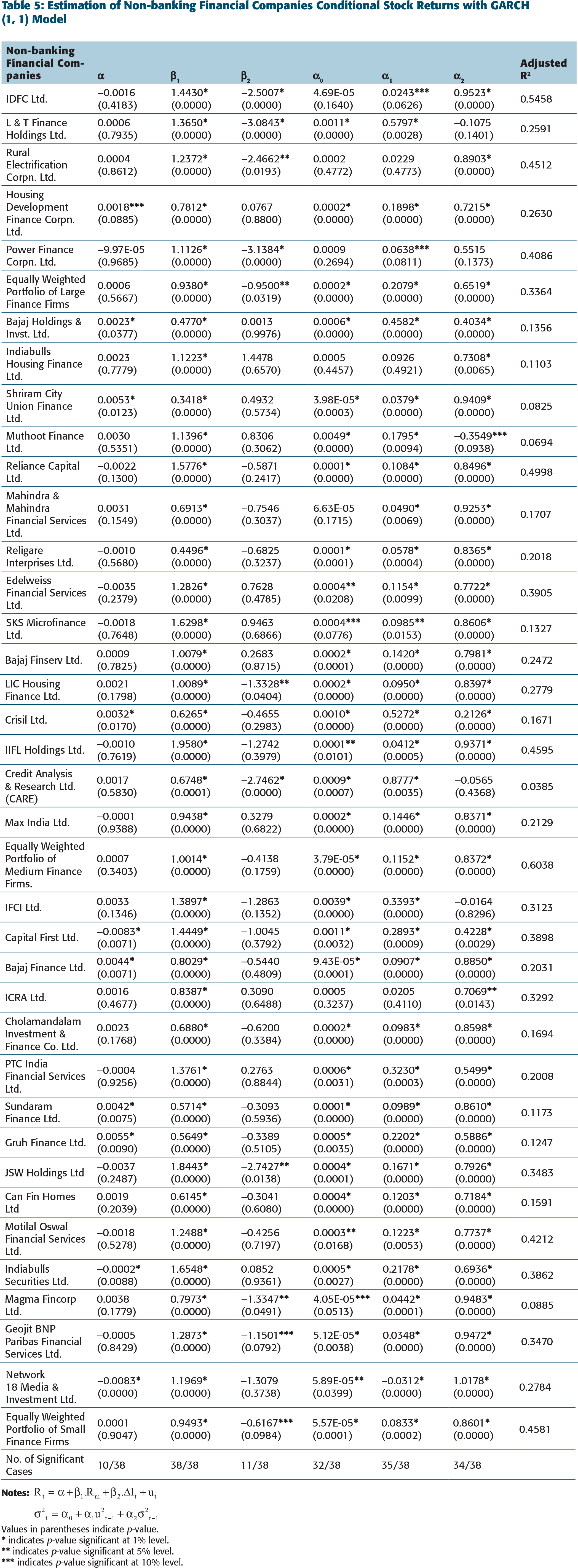
Table 5 presents the results where interest rate sensitivity of individual firm is examined by using the GARCH (1, 1) model. The results shows that α, measuring the effect of market returns on common stock returns of NBFCs, is positive and statistically significant in all cases whereas β₂, the coefficient of interest rate sensitivity, is negative and statistically significant in 11 out of 38 cases. β₂ the coefficient of interest rate sensitivity is statistically significant in 11 out of 38 cases and it is observed that there exists heterogeneity among the interest rate sensitivity of financial companies. The interest rate sensitivity is found to be stronger for large non-banking financial firms (where p-value = 0.0319) and small non-banking financial firms (where p-value = 0.0984) as compared to medium non-banking financial firms. The hypothesis that interest rate sensitivity is uniform across financial sector companies is also rejected, that is, interest rate risk is company specific. According to Flannery and James (1984), the cross-sectional difference in interest rate sensitivity of individual stock returns of financial institutions can be attributed to their balance sheet characteristics or maturity mismatch hypothesis. This is because the financial assets of financial companies represent a significant portion of their total asset and if the duration of their assets and liabilities is not matched, it makes their stock returns interest rate sensitive. The cross-sectional difference in individual NBFC stock returns sensitivity to interest rate can also be attributed to investment preference of their customers, demand of funds by their customer, etc.

In conditional variance equation, α₀ intercept term is statistically significant in 32 out of 38 cases indicating the persistence of average long-term volatility for common stock returns. α₁, ARCH parameter is statistically significant in 35 out of 38 cases implying that volatility of individual NBFC stock returns and portfolio returns is sensitive to the previous period residual variance.α₂, the GARCH parameter is also statistically significant in 34 out of 38 cases implying that volatility of individual firm stock returns and portfolio returns in the current period is strongly related to its volatility in the previous period. Parameters of the conditional variance equationα₀, α₁, and α₂ satisfy non-negativity condition in most cases. α₂ the GARCH parameter is also greater than the ARCH parameter α₁ indicating that the volatility of NBFCs stock returns is more sensitive to its volatility in the previous period than to new shocks in the previous period.

Sum of the ARCH and GARCH parameters is less than one to ensure covariance stationarity and for measuring volatility persistence. Therefore, shocks to stock returns of NBFCs are highly persistent and volatility decays at a slower rate. Non-banking financial industry in India is exposed to undesirable shocks for long periods after they occur. The results show that interest rate changes affect stock returns of NBFCs. However, total interest rate changes consist of two components: anticipated and unanticipated.

The market efficiency theory postulates that the expected value of interest rate changes should already be reflected in the stock prices. Therefore, it is the unanticipated interest rate change which should affect the stock returns. There is inconclusive literature on this aspect. Flannery and James (1984) used unanticipated changes in holding period returns and raw holding period returns. They found identical impact on stock returns for both type of rates, whereas Choi, Elyasiani, and Kopecky (1992) found their results to be different when they used adjusted versus unadjusted interest rate changes. Therefore, this study examines the effect of both total and unanticipated changes in interest rate. To generate the proxy for unexpected interest rate changes, present study uses the ARIMA model of Box–Jenkins methodology. The interest rate series used for calculating residuals of it (unanticipated interest rate changes) under the ARIMA model is found stationary at the first logarithmic difference. The choice of lag under ARIMA model was done by looking at the patterns of autocorrelation (AC) and partial autocorrelation (PAC) graphs. Interest rate series used in the study was found to be significant at lag 1, lag 3, lag 13, and lag 24 only. Hence, interest rate series follows the AR (24,1,0) process. After selecting the ARIMA model, it must be checked for adequacy. The model is adequate if residuals of the model are generally small, randomly distributed, and cannot be used to improve. Residuals of the model selected in present study AR (24) are randomly distributed. The values of AC and PAC pattern qualify the test of significance. The test of significance is that values of AC and PAC should be within .

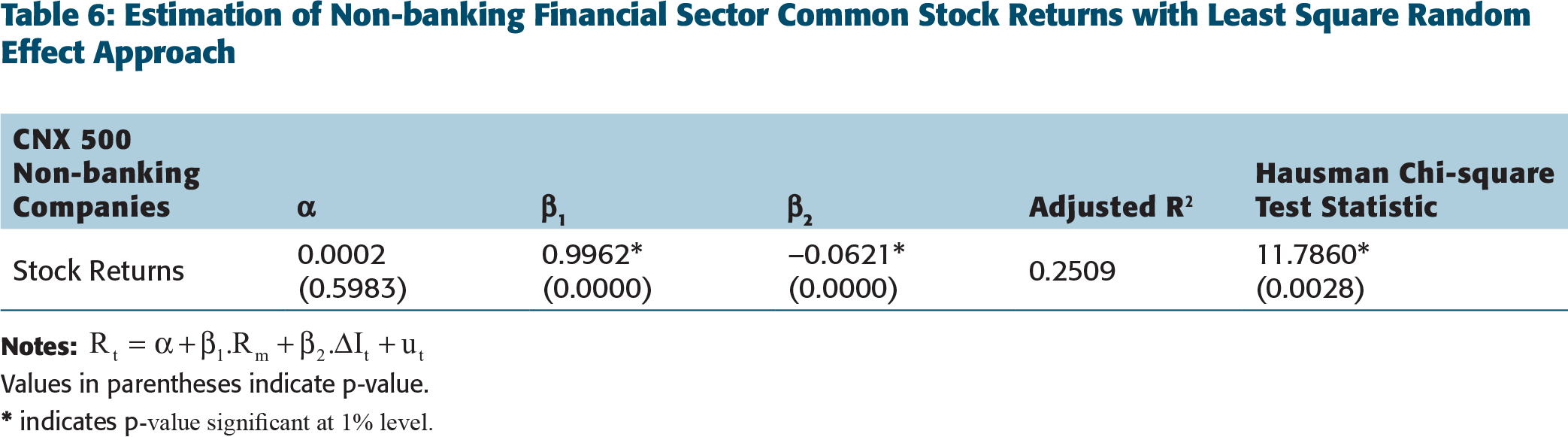
Empirical sensitivity of stock returns of NBFCs to unanticipated changes in interest rate is examined in the following paragraph. The estimates of Table 6 are obtained by using Equation (1).

Table 6:

Estimation of Non-banking Financial Sector Common Stock Returns with Least Square Random Effect Approach

CNX 500 Non-banking Companies	α	β₁	β₂	Adjusted R²	Hausman Chi-square Test Statistic
Stock Returns	0.0002(0.5983)	0.9962^*(0.0000)	−0.0621^*(0.0000)	0.2509	11.7860^*(0.0028)

Notes: $R_{t} = α + β_{1} . R_{m} + β_{2} . Δ I_{t} + u_{t}$

Values in parentheses indicate p-value.

^* indicates p-value significant at 1% level.

Table 6 presents the effect of unanticipated interest rate changes on common stock returns of NBFCs listed in S&P CNX 500 index using the least square estimation random effect approach for panel analysis of data. The results of the table suggest that α, the coefficient of market risk, is positive and statistically significant; β₂, measuring the effect of unanticipated interest rate changes on common stock returns is negative and statistically significant, implying that the NBFCs in India are not protected from unanticipated interest rate risk. Results of the Hausman test statistic are statistically significant at 1 per cent level of significance, suggesting that the least square estimation requires the fixed effect approach for reliable estimation of parameters. The estimates of Table 7 are also obtained by using Equation (1).

Table 7:

Estimation of Non-banking Financial Sector Common Stock Returns with Least Square Fixed Effect Approach

CNX 500 Non-banking Companies	α	β₁	β₂	Adjusted R²
Stock Returns	0.0002(0.5961)	0.9955^*(0.0000)	−0.0622^*(0.0000)	0.2508

Notes: $R_{t} = α + β_{1} . R_{m} + β_{2} . Δ I_{t} + u_{t}$

Values in parentheses indicate p-value.

^* indicates p-value significant at 1% level.

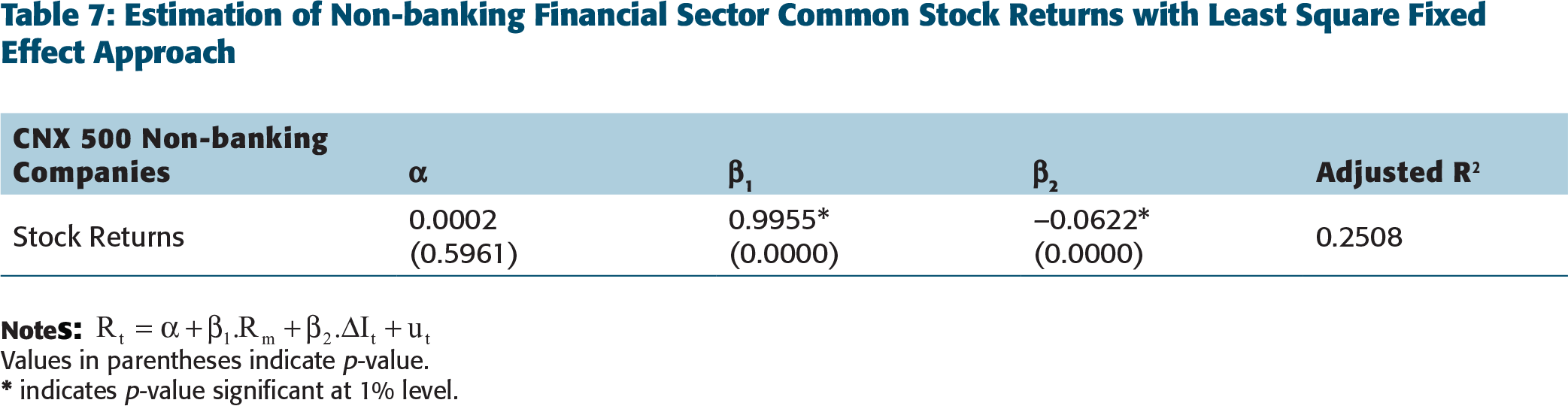
Table 7 presents the effect of unanticipated interest rate changes on common stock returns of NBFCs using the least square estimation fixed effect approach for panel analysis of data. The results obtained by using the least square fixed effect approach are similar to that obtained using random effect. The study further investigated the unanticipated interest rate sensitivity of non-banking financial firms individually. The estimates of Table 8 calculating conditional stock returns of NBFCs were obtained by running separate regression for each company. GARCH (1,1) mode is used to calculate the estimates.

Table 8:

Estimation of Non-banking Financial Companies Conditional Stock Returns with GARCH (1, 1) Model

Non-banking Financial Companies	α	β₁	α₂	α₀	α₁	α₂	Adjusted R²
IDFC Ltd.	−00.16(0.4175)	1.4432(0.0000)	−0.1606(0.0001)	4.88E-05(0.1214)	0.02339(0.0659)	0.9528(0.0000)	0.5480
L & T Finance Holdings Ltd.	−0.0021(0.5342)	1.3036(0.0000)	−0.2669(0.0000)	0.0009(0.0003)	0.2986(0.0010)	0.2519(0.0907)	0.2770
Rural Electrification Corpn. Ltd.	0.0004(0.8839)	1.2433(0.0000)	−0.1328(0.0241)	0.0002(0.4560)	0.0296(0.4149)	0.8718(0.0000)	0.4502
Housing Development Finance Corpn. Ltd.	0.0018(0.0878)	0.7816(0.0000)	0.0108(0.7596)	0.0002(0.0000)	0.1908(0.0000)	0.7202(0.0000)	0.2652
Power Finance Corpn. Ltd.	7.21E-05(0.9774)	1.1138(0.0000)	−0.1531(0.0020)	0.0007(0.2332)	0.0633(0.0606)	0.6138(0.0357)	0.4052
Equally Weighted Portfolio of Large Non-banking Finance Firms	0.0006(0.5406)	0.9392(0.0000)	−0.0449(0.1094)	0.0002(0.0000)	0.2067(0.0000)	0.6569(0.0000)	0.3349
Bajaj Holdings & Invst. Ltd.	0.00233(0.0381)	0.4764(0.0000)	−0.0074(0.8250)	0.0005(0.0000)	0.4580(0.0000)	0.4033(0.0000)	0.1383
Indiabulls Housing Finance Ltd.	0.0024(0.7771)	1.1213(0.0010)	0.1553(0.5937)	0.0005(0.4232)	0.0930(0.4822)	0.7339(0.0027)	0.1657
Shriram City Union Finance Ltd.	0.0053(0.0121)	0.3427(0.0000)	0.0468(0.4290)	3.94E-05(0.0003)	0.0378(0.0000)	0.9413(0.0000)	0.0882
Muthoot Finance Ltd.	0.0033(0.4933)	1.1465(0.0000)	0.0275(0.7452)	0.0049(0.0000)	0.1850(0.0087)	−0.3416(0.0727)	0.0855
Reliance Capital Ltd.	−0.0022(0.1384)	1.5760(0.0000)	−0.0652(0.1030)	0.0001(0.0000)	0.1090(0.0000)	0.8495(0.0000)	0.5019
Mahindra & Mahindra Financial Services Ltd.	0.0031(0.1520)	0.6908(0.0000)	−0.0859(0.1055)	6.48E-05(0.1788)	0.0485(0.0066)	0.9262(0.0000)	0.1802
Religare Interprises Ltd.	−0.0009(0.5820)	0.4487(0.0000)	−0.0753(0.1118)	0.0001(0.0001)	0.0608(0.0004)	0.8334(0.0000)	0.2091
Edelweiss Financial Services Ltd.	−0.0035(0.2367)	1.2835(0.0000)	0.0608(0.4376)	0.0004(0.0213)	0.1154(0.0097)	0.7727(0.0000)	0.3958
SKS Microfinance Ltd.	−0.0018(0.7663)	1.6163(0.0000)	0.0217(0.8828)	0.0004(0.0702)	0.1014(0.0150)	0.8558(0.0000)	0.1454
Bajaj Finserv Ltd.	0.0010(0.7627)	1.0019(0.0000)	−0.0053(0.9620)	0.0002(0.0001)	0.1429(0.0000)	0.7963(0.0000)	0.2545
LIC Housing Finance Ltd.	0.0021(0.1616)	1.0083(0.0000)	−0.1016(0.0236)	0.0002(0.0000)	0.0956(0.0000)	0.8379(0.0000)	0.2809
Crisil Ltd.	0.0032(0.0155)	0.6246(0.0000)	−0.0557(0.1040)	0.0009(0.0000)	0.5334(0.0000)	0.2114(0.0000)	0.1701
IIFL Holdings Ltd.	−0.0009(0.7741)	1.9552(0.0000)	−0.1286(0.2174)	0.0001(0.0088)	0.0428(0.0004)	0.9352(0.0000)	0.4642
Credit Analysis & Research Ltd. (CARE)	0.0028(0.3954)	0.6780(0.0002)	−0.2644(0.0000)	0.0010(0.0015)	0.8394(0.0038)	−0.0620(0.4401)	0.0564
Max India Ltd.	−0.0001(0.9400)	0.9433(0.0000)	0.0133(0.8150)	0.0002(0.0000)	0.1446(0.0000)	0.8371(0.0000)	0.2154
Equally Weighted Portfolio of Medium Non-banking Finance Firms	0.0008(0.3127)	1.0011(0.0000)	−0.0435(0.0534)	3.70E-05(0.0000)	0.1135(0.0000)	0.8399(0.0000)	0.6047
IFCI Ltd.	−0.0032(0.1427)	1.3887(0.0000)	−0.1041(0.0672)	0.0039(0.0000)	0.3336(0.0000)	−0.0138(0.8587)	0.3150
Capital First Ltd.	−0.0084(0.0069)	1.44336(0.0000)	−0.0799(0.3458)	0.0011(0.0030)	0.2898(0.0008)	0.4217(0.0029)	0.3953
Bajaj Finance Ltd.	0.0044(0.0070)	0.8040(0.0000)	−0.0047(0.9289)	9.67E-05(0.0001)	0.0920(0.0000)	0.8831(0.0000)	0.2050
ICRA Ltd.	0.0016(0.4569)	0.8363(0.0000)	−0.0215(0.6215)	0.0005(0.3013)	0.0228(0.3828)	0.6928(0.0163)	0.3342
Cholamandalam Investment & Finance Co. Ltd.	0.0023(0.1746)	0.6879(0.0000)	−0.0508(0.2782)	0.0002(0.0000)	0.0981(0.0000)	0.8597(0.0000)	0.1725
PTC India Financial Services Ltd.	−0.0004(0.9215)	1.3831(0.0000)	0.0517(0.81119)	0.0006(0.0034)	0.3212(0.0003)	0.5502(0.0000)	0.2147
Sundaram Finance Ltd.	0.0042(0.0070)	0.5715(0.0000)	−0.0295(0.4924)	0.0001(0.0000)	0.0988(0.0000)	0.8611(0.0000)	0.1204
Gruh Finance Ltd.	0.0055(0.0095)	0.5643(0.0000)	−0.0048(0.8921)	0.0005(0.0034)	0.2217(0.0000)	0.5885(0.0000)	0.1284
JSW Holdings Ltd.	−0.0038(0.2224)	1.8514(0.0000)	−0.1310(0.1218)	0.0004(0.0000)	0.1685(0.0000)	0.7880(0.0000)	0.3512
Can Fin Homes Ltd.	0.0019(0.2035)	0.6144(0.0000)	−0.0161(0.7209)	0.0004(0.0000)	0.1201(0.0000)	0.7177(0.0000)	0.1619
Motilal Oswal Financial Services Ltd.	−0.0018(0.5246)	1.2497(0.0000)	−0.0275(0.7509)	0.0003(0.0165)	0.1215(0.0053)	0.7759(0.0000)	0.4257
Indiabulls Securities Ltd.	−0.0082(0.0089)	1.6473(0.0000)	−0.0331(0.6744)	0.0005(0.0030)	0.2212(0.0000)	0.6918(0.0000)	0.3926
Magma Fincorp Ltd.	0.0037(0.1883)	0.8012(0.0000)	−0.0696(0.1322)	4.03E-05(0.0526)	0.0441(0.0001)	0.9488(0.0000)	0.0929
Geojit BNP Paribas Financial Services Ltd.	−0.0005(0.8508)	1.2851(0.0000)	−0.1325(0.0034)	5.01E-05(0.0042)	0.0349(0.0000)	0.9474(0.0000)	0.3539
Network 18 Media & Investment Ltd.	−0.0081(0.0000)	1.1990(0.0000)	−0.0847(0.4147)	5.65E-05(0.0321)	−0.0306(0.0000)	1.0177(0.0000)	0.2852
Equally Weighted Portfolio of Small Non-banking Finance Firms	0.0001(0.8812)	0.9509(0.0000)	−0.0454(0.0587)	5.48E-05(0.0001)	0.0825(0.0002)	0.8617(0.0000)	0.4578
Number of significant cases	10/38	38/38	12/38	32/38	35/38	34/38

Notes: $R_{t} = α + β_{1} . R_{m} + β_{2} . Δ I_{t} + u_{t}$

$σ^{2}_{t} = α_{0} + α_{1} u^{2}_{t - 1} + α_{2} σ^{2}_{t - 1}$

Values in parentheses indicate p-value.

^* indicates p-value significant at 1% level.

^** indicates p-value significant at 5% level.

^*** indicates p-value significant at 10% level.

Table 8 presents the results of the GARCH (1,1) model in which sensitivity of non-banking financial institution’s conditional stock returns is examined with market returns and unanticipated changes in interest rate. α measuring the effect of market returns on common stock returns of NBFCs is positive and statistically significant in all cases whereas β₂ the coefficient of unanticipated interest rate sensitivity is negative and statistically significant in 12 out of 38 cases. When unanticipated changes in interest rate are used in lieu of actual interest rate changes, not much difference is observed in the significance coefficients except for magnitude. The impact of actual interest rate changes is more than the impact of unanticipated interest rate changes in absolute terms. This difference in the magnitude of impact arises because actual data incorporate movement in both anticipated and unanticipated components of interest rate. Results of this study are consistent with the findings of Drakos (2001) which suggested that bank’s stock returns listed in Athens Stock Exchange have significant exposure with interest rate movements. The coefficient of interest rate risk was significant in case of seven out of nine banks, that is, interest rate risk is bank specific. The number of variables relating to balance sheet of the select banks is correlated with interest rate variability but working capital is found to be the statistically preferred determinant.

Interest rate sensitivity of individual firms examined by using GARCH (1,1) model is found to be different for different firms (for some firms, it was significantly positive or negative; for others it was not). There are a number of possible explanations proposed in literature as to why finance firms may exhibit interest rate risk heterogeneity. According to Flannery and James (1984), the cross-sectional difference in individual bank stock returns sensitivity to interest rate can be attributed to their balance sheet characteristics or maturity mismatch hypothesis because financial assets of financial companies represent a significant portion of their total assets and if the duration of their assets and liabilities is not matched, it makes their stock returns interest rate sensitive. Flannery and James (1984) analysis was based on the concept of nominal contracting hypothesis. The nominal contacting hypothesis postulates that a firm’s holding of nominal assets plays an important role in explaining the behaviour of common stock returns through the redistributive effects of unanticipated inflation and unanticipated changes in expected inflation (French, Ruback, & Schwert, 1983). If movements in the term structure of interest rates (unanticipated changes in the level of interest rates) result primarily from changes in inflationary expectations, then the nominal contracting hypothesis implies a relation between common stock returns and interest rate changes. In particular, the interest rate sensitivity of a firm’s common stock returns will depend upon the firm’s holding of net nominal assets and maturity composition of net nominal assets held. The higher the proportion of net nominal assets and the longer the maturity of net nominal assets held, the more sensitive should be the firm’s common stock returns to interest rate changes. The cross-sectional variation in the interest rate sensitivity of financial firms is analysed by using Equation (4). The estimates of Table 9 are obtained by running separate panel regression for each financial variable individually. β_2i in Equation (4) and β₂ in Equation (2) are related. The interest rate risk coefficient (β₂) is modelled as a function of financial variables, whereβ₂’s of individual firms are regressed on the financial variable obtained from their balance sheet.

Table 9:

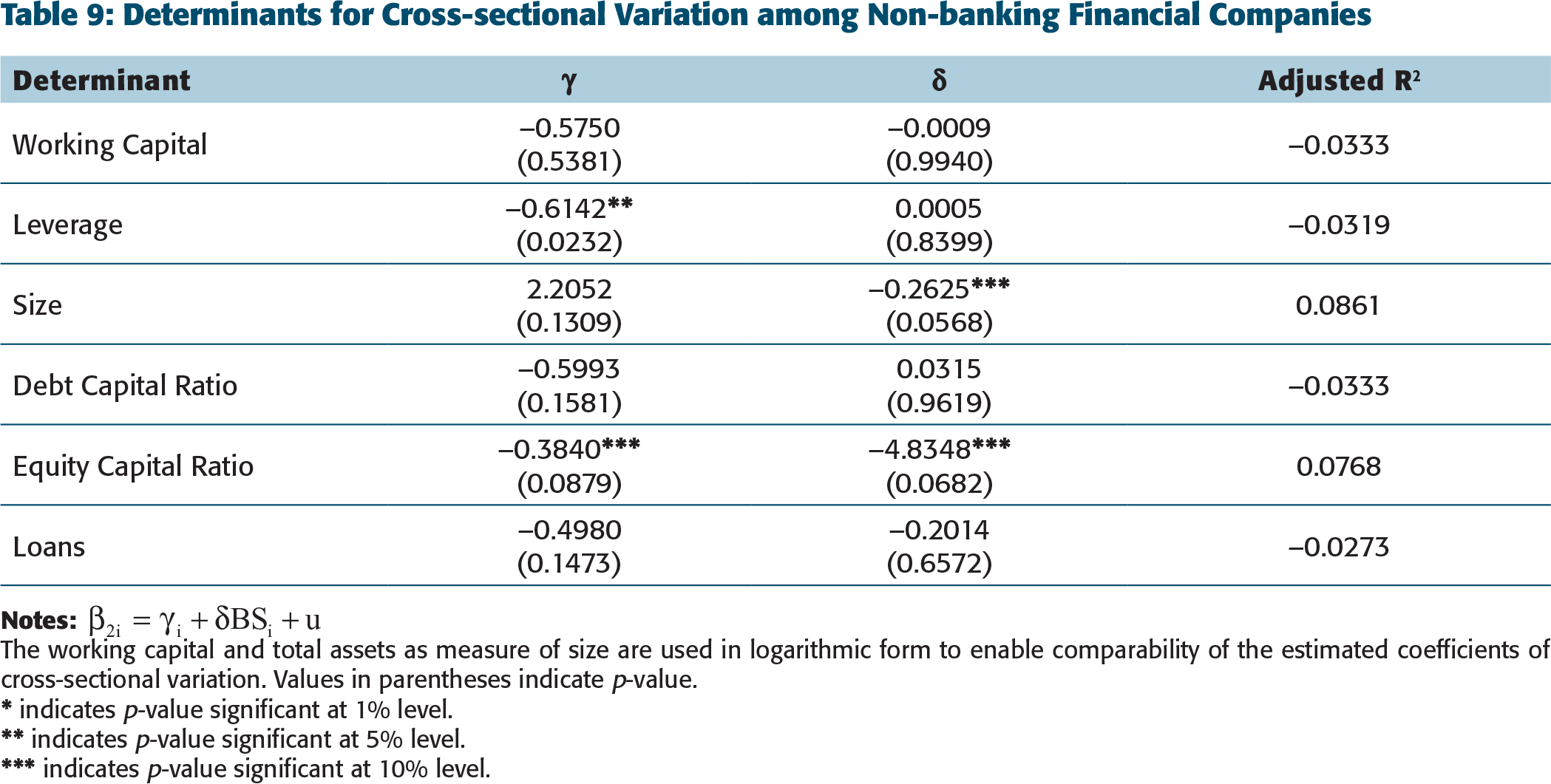
Determinants for Cross-sectional Variation among Non-banking Financial Companies

Determinant	γ	δ	Adjusted R²
Working Capital	−0.5750(0.5381)	−0.0009(0.9940)	−0.0333
Leverage	−0.6142^**(0.0232)	0.0005(0.8399)	−0.0319
Size	2.2052(0.1309)	−0.2625^***(0.0568)	0.0861
Debt Capital Ratio	−0.5993(0.1581)	0.0315(0.9619)	−0.0333
Equity Capital Ratio	−0.3840^***(0.0879)	−4.8348^***(0.0682)	0.0768
Loans	−0.4980(0.1473)	−0.2014(0.6572)	−0.0273

Notes: $β_{2 i} = γ_{i} + δ B S_{i} + u$

The working capital and total assets as measure of size are used in logarithmic form to enable comparability of the estimated coefficients of cross-sectional variation. Values in parentheses indicate p-value.

^* indicates p-value significant at 1% level.

^** indicates p-value significant at 5% level.

^*** indicates p-value significant at 10% level

Table 9 presents the results relating to the investigation of determinants that account for cross-sectional variation between non-banking financial firms employed in the study. The main objective of the analysis is to explore the balance sheet variables that explain the highest proportion of interest rate risk variability. The results show that working capital, leverage, debt capital proportion, and loans have no explanatory power, whereas size and equity capital proportion of the firm explain a significant proportion of the variation in interest rate sensitivity across non-banking financial firms. Working capital and debt capital ratio have the lowest explanatory power, whereas size of the firm (8.61%) exhibits the highest explanatory power for variation in the interest rate sensitivity across non-banking financial firms listed in S&P CNX 500. It can also be observed from the results that when equity as a component of leverage is considered individually, it exhibits significant explanatory power. Thus, the absolute level of equity matters for each financial firm’s interest rate sensitivity but its ratio with debt does not matter and explains a significant proportion of interest rate sensitivity variation. In other words, absolute levels of financing for non-banking financial firms determine their interest rate risk.

Overall, the size of the firm as measured by total assets of the firm is the statistically preferred determinant having highest level of significance and coefficient of determination. The possible reason for this may be that firms with higher levels of assets have the greater chance of potential loss from unexpected increase and thus greater interest rate sensitivity.

SUMMARY AND CONCLUSIONS

The issue of interest rate sensitivity of common stock returns is of major interest for regulators, banks and academicians and for that reason a voluminous amount of literature has explored the issue. In this study, interest rate sensitivity of NBFCs stock returns is analysed from 1 January 1996 to 30 August 2014. This period is characterized by the deregulation of interest rate in India. Administrative restrictions on interest rates have been steadily eased since 1993. The sample for the purpose of study consists of 35 NBFCs forming part of S&P CNX 500 index that has continuous available prices for the period under consideration. The basic data used for the study are secondary in nature. The data publicly disseminated by NSE and RBI through their respective websites is the main source of data which is supplemented with PROWESS database maintained by Centre for Monitoring of Indian Economy. Weekly stock returns for individual firm were used to create equally weighted portfolio returns.

To examine the relationship between interest rate movements and stock returns, two alternative econometric approaches were followed. First, interest rate sensitivity of stock returns was tested by pooling information across the sample employed in the study by using panel regression analysis. Second, in a single equation framework, the interest rate sensitivity of individual firm stock returns was tested by using the GARCH (1, 1) model to test the uniformity hypothesis of interest rate effect. The study also investigated the determinants of interest rate risk heterogeneity for financial firms due to rejection of the uniformity hypothesis.

The effect of interest rate on stock returns movement is evident from the results. Coefficient of market risk is found to be positive and statistically significant, whereas the effect of interest rate changes on common stock returns is found to be negative. The reason for negative relationship between stock returns and interest rate movements may be that when interest rates are hiked, investors transfer their money out of the stock market, believing that higher borrowing costs will affect balance sheet negatively and thus resulting in devaluating the stock price (Singh & Arora, 2010).

Interest rate sensitivity of large financial institutions, medium financial institutions, and small financial institutions is also found to be different. Interest rate sensitivity is found to be stronger for large firms as compared to small- and medium-sized firms. Interest rate effect is not uniform across firms considered in the study. Estimation results for the variance equation in the GARCH (1, 1) model suggest that the volatility for individual firm stock returns is time-variant. The implication is that market has a memory longer than one period and volatility is more sensitive to its own lagged values than to new surprises in the market.

When the impact of unanticipated interest rate changes is analysed in place of total interest rate changes on the stock returns, little difference is observed in the significance coefficients (p-value); the only significant difference observed from the results is that the impact of actual interest rate changes on stock returns is more than the impact of unanticipated interest rate changes in absolute terms. This difference in magnitude of impact arises because actual data incorporate movement in both anticipated and unanticipated components of interest rate. The size of the firm as measured by total assets of the firm is the statistically preferred determinant having highest level of significance and coefficient of determination for cross-sectional variation in the interest rate sensitivity of NBFCs. Results of the present study lends support to the Stone’s (1974) dual index model that incorporation of interest rate as an extra factor adds substantial power to the model in explaining stock returns. A limitation of the present study is that it is based on separate regression for each firm. Further research can be undertaken to bring together all firms into one model with random effects for intercepts and slope being modelled as a function of firm’s characteristics.

DECLARATION OF CONFLICTING INTERESTS

The authors declared no potential conflicts of interest with respect to the research, authorship and/or publication of this article.

FUNDING

The authors received no financial support for the research, authorship and/or publication of this article.

APPENDIX

Table A1:

List of Financial Companies with Average Market Capitalization

Company Name	Average Market Capitalization( millions)	Average Market Capitalization( Crores)
Large Non-banking Financial Firm’s Portfolio:
Housing Development Finance Corpn. Ltd.	432,461.6509	43,246.16509
I D F C Ltd.	169,782.3735	16,978.23735
L & T Finance Holdings Ltd.	107,964.3909	10,796.43909
Power Finance Corpn. Ltd.	239,556.1826	23,955.61826
Rural Electrification Corpn. Ltd.	196,278.4029	19,627.84029
Medium Non-banking Finance Firm’s Portfolio:
Bajaj Finserv Ltd.	81,506.91076	8,150.691076
Bajaj Holdings & Invst. Ltd.	94,496.89352	9,449.689352
Credit Analysis & Research Ltd.	22,621.07739	2,262.107739
Crisil Ltd.	22,014.91743	2,201.491743
Edelweiss Financial Services Ltd.	31,901.36741	3,190.136741
I I F L Holdings Ltd.	24,252.94918	2,425.294918
Indiabulls Housing Finance Ltd.	88,396.03172	8,839.603172
L I C Housing Finance Ltd.	37,581.97714	3,758.197714
Mahindra & Mahindra Financial Services Ltd.	62,103.31609	6,210.331609
Max India Ltd.	22,625.41446	2,262.541446
Muthoot Finance Ltd.	58,493.42983	5,849.342983
Reliance Capital Ltd.	85,056.3721	8,505.63721
Religare Enterprises Ltd.	46,202.73715	4,620.273715
S K S Microfinance Ltd.	24,307.88028	2,430.788028
Shriram City Union Finance Ltd.	26,255.87081	2,625.587081
Small Non-banking Financial Firm’s Portfolio:
Bajaj Finance Ltd.	13,918.31125	1,391.831125
Can Fin Homes Ltd.	1,283.018101	128.3018101
Capital First Ltd.	13,900.12564	1,390.012564
Cholamandalam Investment & Finance Co. Ltd.	8,593.167064	859.3167064
Geojit B N P Paribas Financial Services Ltd.	6,220.944238	622.0944238
Gruh Finance Ltd.	15,648.84839	1,564.884839
I C R A Ltd.	10,709.66321	1,070.966321
I F C I Ltd.	19,335.38293	1,933.538293
Indiabulls Securities Ltd.	6,175.759672	617.5759672
J S W Holdings Ltd.	8,124.378771	812.4378771
Magma Fincorp Ltd.	7,317.167093	731.7167093
Motilal Oswal Financial Services Ltd.	18,665.96569	1,866.596569
Network18 Media & Invst. Ltd.	19,618.06566	1,961.806566
P T C India Financial Services Ltd.	9,239.991061	923.9991061
Sundaram Finance Ltd.	16,721.74233	1,672.174233

Table A2:

Descriptive Statistics of Returns Series

Non-banking Financial Companies	Mean	Maximum	Minimum	Std. Dev.	Skewness	Kurtosis	Jarque–Bera	Probability
IDFC Ltd.	0.0015	0.2741	−0.3449	0.0670	−0.0875	5.2564	100.7325	0.00
L & T Finance Holdings Ltd.	0.0017	0.2644	−0.1285	0.0551	1.1524	6.8081	131.2645	0.00
Rural Electrification Corpn. Ltd.	0.0026	0.1886	−0.2509	0.0620	−0.0549	3.7351	7.7578	0.02
Housing Development Finance Corpn. Ltd.	0.0038	0.2355	−0.1888	0.0489	0.1784	5.1688	195.8606	0.00
Power Finance Corpn. Ltd.	0.0021	0.2467	−0.2132	0.0630	−0.0322	3.8216	11.0946	0.00
Equally Weighted Portfolio of Large Finance Firms	0.0021	0.2574	−0.2523	0.0467	0.0479	5.2726	209.7617	0.00
Bajaj Holdings & Invst. Ltd.	0.0011	0.2309	−0.8862	0.0574	−3.8210	61.6878	142,003.7000	0.00
Indiabulls Housing Finance Ltd.	0.0076	0.1753	−0.1754	0.0654	−0.0129	4.1563	3.1770	0.20
Shriram City Union Finance Ltd.	0.0080	0.4546	−0.2450	0.0536	1.5159	16.3033	3,800.9520	0.00
Muthoot Finance Ltd.	0.0006	0.2407	−0.2350	0.0684	0.1532	4.4985	16.8627	0.00
Reliance Capital Ltd.	0.0018	0.4233	−0.2999	0.0797	0.2027	5.7593	315.3313	0.00
Mahindra & Mahindra Financial Services Ltd.	0.0041	0.2128	−0.1910	0.0544	0.0670	4.2200	27.6813	0.00
Religare Interprises Ltd.	−0.0013	0.2306	−0.1271	0.0393	1.2786	10.4701	916.9391	0.00
Edelweiss Financial Services Ltd.	−0.0031	0.3409	−0.2892	0.0728	0.7315	7.3351	305.2708	0.00
SKS Microfinance Ltd.	−0.0067	0.3681	−0.3115	0.0985	−0.0522	4.6631	24.2985	0.00
Bajaj Finserv Ltd.	0.0016	0.2996	−0.5826	0.0733	−1.2991	16.4819	2,560.6110	0.00
LIC Housing Finance Ltd.	0.0038	0.2595	−0.3498	0.0642	0.1240	6.5296	507.5594	0.00
Crisil Ltd.	0.0050	0.3761	−0.3280	0.0559	0.9260	10.2154	2,249.7350	0.00
IIFL Holdings Ltd.	0.0044	0.5022	−0.4488	0.0974	0.4417	7.4303	411.5569	0.00
Credit Analysis & Research Ltd. (CARE)	0.0035	0.2009	−0.2081	0.0543	−0.3430	6.7235	51.9641	0.00
Max India Ltd.	0.0028	0.6568	−0.6502	0.0796	0.4288	13.5515	4,543.4440	0.00
Equally Weighted Portfolio of Medium Finance Firms.	0.0030	0.1941	−0.2088	0.0388	0.0187	5.6537	285.5466	0.00
IFCI Ltd.	−0.0001	0.5657	−0.3921	0.0866	0.7237	8.0773	1,130.0400	0.00
Capital First Ltd.	−0.0035	0.3920	−0.2943	0.0786	0.2854	5.8792	123.1345	0.00
Bajaj Finance Ltd.	0.0037	0.3331	−0.4428	0.0650	0.0339	9.0802	1,498.9460	0.00
ICRA Ltd.	0.0031	0.1922	−0.2248	0.0506	0.0839	5.7012	117.4956	0.00
Cholamandalam Investment & Finance Co. Ltd.	0.0023	0.3856	−0.2794	0.0657	0.7213	7.2779	826.3107	0.00
PTC India Financial Services Ltd.	0.0030	0.3980	−0.1243	0.0624	1.8994	12.4730	772.5849	0.00
Sundaram Finance Ltd.	0.0031	0.3750	−0.2663	0.0525	1.3271	11.6707	3,333.5830	0.00
Gruh Finance Ltd.	0.0083	0.3351	−0.2488	0.0526	0.4106	8.2169	604.2887	0.00
JSW Holdings Ltd.	0.0026	0.6506	−0.3193	0.1007	1.2736	8.9134	827.4031	0.00
Can Fin Homes Ltd.	0.0029	0.3562	−0.2534	0.0532	0.7938	9.1939	1,657.5090	0.00
Motilal Oswal Financial Services Ltd.	0.0002	0.2976	−0.1989	0.0728	0.3067	4.8596	57.9921	0.00
Indiabulls Securities Ltd.	−0.0040	0.5495	−0.5996	0.0891	0.0926	12.5607	1,272.5590	0.00
Magma Fincorp Ltd.	0.0057	0.3019	−0.2098	0.0744	0.7795	5.1138	154.9293	0.00
Geojit BNP Paribas Financial Services Ltd.	0.0028	0.4168	−0.4672	0.0755	0.4646	9.7976	937.4958	0.00
Network 18 Media & Investment Ltd.	−0.0050	0.3458	−0.3053	0.0781	0.4978	5.6651	133.2087	0.00
Equally Weighted Portfolio of Small Finance Firms	0.0024	0.6568	−0.6502	0.0752	0.4158	16.1859	7,076.8850	0.00

Figure 1:

Implicit Yield at Cut-off Price on 91-days Treasury Bills

References

Alam

M. M.

Salahuddin

M. G.

(2009). Relationship between interest rate and stock price: Empirical evidence from developed and developing countries. International Journal of Business and Management , 4(3), 43–51.

Asprem

(1989). Stock prices, asset portfolios and macroeconomic variables in ten European countries. Journal of Banking and Finance , 13(4–5), 589–612.

Ballester

Ferrer

Gonzalez

(2011). Linear and non linear interest rate sensitivity of Spanish banks. The Spanish Review of Financial Economics , 9(2), 35–48.

Ballester

Ferrer

Gonzalez

Soto

G. M.

(2009). Determinants of interest rate exposure of Spanish banking industry (Working Paper No. WP-EC 2009-07). Spain: Documentos de Trabajo, Departmento de Analisis Economico y Finanzas.

Benink

H. A.

Wolff

C. C.

(2000). Survey data and the interest rate sensitivity of US bank stock returns. Economic Notes , 29(2), 201–213.

Bollerslev

Chou

R. Y.

Kroner

K. F.

(1992). ARCH modeling in finance: A review of theory and empirical evidence. Journal of Econometrics , 52, 5–59.

Brooks

(2002). Introductory econometrics for finance . Cambridge, UK: Cambridge University Press.

Choi

Jen

F. C.

(1991). The relation between stock returns and short-term interest rates. Review of Quantitative Finance and Accounting , 1, 75–89.

Choi

J. J.

Elyasiani

Kopecky

K. J.

(1992). The sensitivity of bank stock returns to market, interest and exchange rate risks. Journal of Banking and Finance , 16(5), 983–1004.

10.

Dinesis

Staikouras

S. K.

(1998). Interest rate changes and common stock returns of financial institutions: Evidence from the UK. The European Journal of Finance , 4(2), 113–127.

11.

Drakos

(2001). Interest rate risk and bank common stock returns: Evidence from the Greek banking sector. London: Department of Economics, London Guildhall University.

12.

Flannery

M. J.

James

C. M.

(1984). The effect of interest rate changes on the common stock returns of financial institutions. The Journal of Finance , 39(4), 1141–1153.

13.

French

K. R.

Ruback

R. S.

Schwert

G. W.

(1983). Effects of nominal contracting on stock returns. Journal of Political Economy , 91(1), 70–96.

14.

Hanke

J. E.

Wichern

D. W.

(2009). Business forecasting (8th ed.). New Delhi: PHI Learning Private Limited.

15.

Hausman

J. A.

(1978). Specification tests in econometrics. Econometrica , 46(6), 1251–1271.

16.

Judge

G. G.

Hill

R. C.

Griffiths

Lutkepoul

Lee

T.-C.

(1982). Introduction to the theory and practice of econometrics . New York, NY: John Wiley & Sons.

17.

Kasman

Vardar

Gokce

(2011). The impact of interest rate and exchange rate volatility on bank’s stock returns and volatility: Evidence from Turkey. Economic Modelling , 28(3), 1328–1334.

18.

Kwan

S. H.

(1991). Re-examination of interest rate sensitivity of commercial bank stock returns using a random coefficient model. Journal of Financial Services Research , 5(1), 61–76.

19.

Latha

Gupta

Ghosh

(2016). Interest rate sensitivity of stock returns: A case study of textile sector in India. Asian Journal of Multidisciplinary Studies , 4(4), 56–61.

20.

Levin

Lin

C.-F.

Chu

C.-S. J.

(2002). Unit root tests in panel data: Asymptotic and finite-sample properties. Journal of Econometrics , 108(1), 1–24.

21.

Lynge

M. J.

Zumwalt

J. K.

(1980). An empirical study of the interest rate sensitivity of commercial bank returns: A multi-index approach. The Journal of Financial and Quantitative Analysis , 15(3), 731–742.

22.

Martin

J. D.

Keown

A. J.

(1977). Interest rate sensitivity and portfolio risk. The Journal of Financial and Quantitative Analysis , 12(2), 181–195.

23.

Moss

J. D.

Moss

G. J.

(2010). Variables explaining bank stock prices. The Journal of Applied Business Research , 26(4), 9–12.

24.

Park

Choi

B. P.

(2011). Interest rate sensitivity of US property/liability insurer stock returns. Managerial Finance , 37(2), 134–150.

25.

Patnaik

Shah

(2002). Interest-rate risk in the Indian banking system (Working Paper No. 92). Indian Council for Research on International Economic Relations.

26.

Ross

S. A.

(1976). The arbitrage theory of capital asset pricing. Journal of Economic Theory , 13(3), 341–360.

27.

Singh

Arora

V. P.

(2010). Interest rates and stock movements in three major Asian countries—India, China and Japan . Retrieved from http://ssrn.com/abstract=1574201

28.

Stone

B. K.

(1974). Systematic interest-rate risk in a two-index model of returns. The Journal of Financial and Quantitative Analysis , 9(5), 709–721.

Interest Rate Sensitivity of Non-banking Financial Sector in India

Abstract

Executive Summary

Keywords

OBJECTIVES OF THE STUDY

Data and Sources

Classification of Sample Financial Companies

Interest Rate Proxy

Market Proxy

LITERATURE REVIEW

RESEARCH METHODOLOGY

Panel Regression Analysis

GARCH (1, 1) Model

Correlation Coefficients between Market Returns and Interest Rate Changes

EMPIRICAL RESULTS

Estimation of NBFCs Common Stock Returns with Least Square Random Effect Approach

Estimation of NBFCs Common Stock Returns with Least Square Fixed Effect Approach

Estimation of Non-banking Financial Companies Conditional Stock Returns with GARCH (1, 1) Model

Estimation of Non-banking Financial Sector Common Stock Returns with Least Square Random Effect Approach

Estimation of Non-banking Financial Sector Common Stock Returns with Least Square Fixed Effect Approach

Estimation of Non-banking Financial Companies Conditional Stock Returns with GARCH (1, 1) Model

Determinants for Cross-sectional Variation among Non-banking Financial Companies

SUMMARY AND CONCLUSIONS

DECLARATION OF CONFLICTING INTERESTS

FUNDING

APPENDIX

List of Financial Companies with Average Market Capitalization

Descriptive Statistics of Returns Series

Implicit Yield at Cut-off Price on 91-days Treasury Bills

References