Sage Journals: Discover world-class research

Abstract

Executive Summary

Cross-sectional volatility measures dispersion of security returns at a particular point of time. It has received very little focus in research. This article studies the cross-section of volatility in the context of economies of Brazil, Russia, India, Indonesia, China, South Korea, and South Africa (BRIICKS). The analysis is done in two parts. The first part deals with systematic volatility (SV), that is, cross-sectional variation of stock returns owing to their exposure to market volatility measure (French, Schwert, & Stambaugh, 1987). The second part deals with unsystematic volatility (UV), measured by the residual variance of stocks in a given period by using error terms obtained from Fama–French model.

The study finds that high SV portfolios exhibit low returns in case of Brazil, South Korea, and Russia. The risk premium is found to be statistically significantly negative for these countries. This finding is consistent with Ang et al. and is indicative of hedging motive of investors in these markets. Results for other sample countries are somewhat puzzling. No significant risk premiums are reported for India and China. Significantly positive risk premiums are observed for South Africa and Indonesia. Further, capital asset pricing model (CAPM) seems to be a poor descriptor of returns on systematic risk loading sorted portfolios while FF is able to explain returns on all portfolios except high SV loading portfolio (i.e., P1) in case of South Africa which seems to be an asset pricing anomaly.

It is further observed that high UV portfolios exhibit high returns in all the sample countries except China. In the Chinese market, the estimated risk premium is statistically significantly negative. This negative risk premium is inconsistent with the theory that predicts that investors demand risk compensation for imperfect diversification. The remaining sample countries show significantly positive risk premium. CAPM does not seem to be a suitable descriptor for returns on UV sorted portfolios. The FF model does a better job but still fails to explain the returns on high UV sorted portfolio in case of Brazil and China and low UV sorted portfolio in South Africa.

The findings are relevant for global fund managers who plan to develop emerging market strategies for asset allocation. The study contributes to portfolio management as well as market efficiency literature for emerging economies.

Keywords

BRIICKS Economies Cross-sectional Volatility Systematic Volatility Unsystematic Volatility CAPM Fama–French Model Risk Premium

Stock market anomalies are of great interest to investment analysts and portfolio managers. The capital asset pricing model (CAPM) (Black, 1972; Lintner, 1965; Sharpe, 1964) is a widely used model for pricing securities in the stock market. As per this model, a stock return can be explained by its sensitivity to the market factor. But, the CAPM has been questioned by many researchers. Accordingly, there are many CAPM anomalies. The important ones are book-to-market value (Rosenberg, Reid, & Lanstein, 1985; Stattman, 1980), size (Banz, 1981), earning–price ratio (Basu, 1983), return reversals (De Bondt & Thaler, 1985, 1987), leverage (Bhandari, 1988), and return momentum (Jegadeesh & Titman, 1993). Fama and French (1993) gave a three-factor model by including two additional factors, that is, the size factor and the value factor, and showed that this three-factor model explained almost all important CAPM anomalies except stock momentum. Therefore, the FF model is a widely used asset pricing model. But, portfolio managers continue to identify new anomalies where abnormal profit possibilities appear to exist.

Many researchers have studied volatility for mature as well as emerging markets (see Adrian & Rosenberg, 2008; Campbell, Lettau, Malkiel, & Xu, 2001; Ederington & Guan, 2005; Glosten, Jagannathan, & Runkle, 1993; Merton, 1973; Schwert, 1989; Sehgal & Vijayakumar, 2008). It is now widely accepted that volatility is stochastic (see Wiggins, 1987; Hull & White, 1987). A new stock return anomaly on which very limited work is available is cross-sectional volatility. Prior empirical work had studied the cross-section of volatility in two parts, that is, systematic volatility (SV) and unsystematic volatility (UV). SV refers to market-wide volatility. When an investment opportunity set varies over time, the Intertemporal CAPM of Merton (1973) shows that the expected return on risky asset is determined by the conditional covariances between the asset returns and innovations in the state variables that can act as a hedge against varying investment opportunities. Campbell (1993, 1996) suggested that risk-averse investors wanted to hedge against changes in market volatility but his model did not directly study the impact of changes in market volatility on expected asset returns. Chen (2002) extended Campbell’s model and directly incorporated changes in market volatility to study its impact on expected asset returns.

Motivated by these studies, we use a simple model where market volatility is a state variable. Market volatility can be estimated using historical volatility and implied volatility measures. Historical volatility (or realized volatility) is a measure of past price movements of the underlying asset, whereas implied volatility reflects market expectations regarding the asset’s future volatility. Variance of asset returns is often used to calculate historical volatility. It is based on the closing prices of the reference period and totally ignores the price information within the reference period. Therefore, an alternate measure is range estimator of historical volatility. Historical volatility may not accurately reflect future volatility, and therefore implied volatility is often calculated using option prices. Unsystematic volatility (UV) or idiosyncratic volatility is specific to an individual company. It is measured by the residual variance of stocks in a given period using the error terms obtained from a standard asset pricing model such as the CAPM or the Fama–French three-factor model (see Ang, Hodrick, Xing, & Zhang, 2006; Cutler, 1989).

While considerable research has been done on the time series relationship between expected market return and market volatility (see French, Schwert, & Stambaugh,1987; Glosten et al., 1993), limited empirical evidence is available on cross-sectional volatility and that too mostly for the developed markets. Although the findings are interesting, developed markets alone should not determine the role of cross-sectional volatility. It is important to study other stock markets around the world that can provide further evidence. Therefore, this article focuses on the previously neglected markets: the emerging markets. It should be interesting to look at the evidence from these markets as the empirical results, at times, might conflict with the available international work. This article focuses on economies of Brazil, Russia, India, and China (BRIC) and three other markets: Indonesia, South Korea, and South Africa. Hence, for our study, we use the emerging market acronym BRIICKS—Brazil, Russia, India, Indonesia, China, South Korea, and South Africa representing the world’s major emerging economies. These markets are gaining importance because global investors tend to combine them with their developed market investments for risk diversification purpose.

In emerging markets, there is a virtual absence of empirical work on cross-sectional volatility anomaly.¹

There is only one study by Sehgal et al. (2012) on Indian stock market using data in INR.

It is important for policy makers, global investment managers as well as the academia to understand if there are any significant differences in the cross-sectional volatility patterns in stock returns for mature and emerging markets and whether these observable patterns can be explained by common risk factors. Any empirical finding on the issue shall not only provide better insights about market efficiency and asset pricing but also has implications for designing investment strategy.

The main objective of this article is to fill the gap in asset pricing literature. An attempt has been made to find answers to the following questions:

Is there any return differential among SV loading sorted portfolios?

Is there any return differential among portfolios sorted on the basis of UV?

Do the asset pricing models like the CAPM and the Fama–French Model explain the returns on the portfolios formed on the basis of volatility?

LITERATURE REVIEW

French et al. (1987) studied the intertemporal relationship between expected risk premium on stock market portfolio and stock market volatility using the data relating to the New York Stock Exchange (NYSE) common stocks. The sample period of the study was from January 1928 to December 1984. Monthly variance of market return was calculated as the sum of the squared daily returns plus twice the sum of the products of adjacent returns. They decomposed the computed monthly volatility estimate into predictable and unpredictable components using univariate autoregressive integrated moving average models. Their results demonstrated a significantly negative relationship between expected risk premium and unpredictable volatility. This negative ex post relation was interpreted as an indirect evidence of a positive ex ante relationship between risk premium and volatility. Glosten et al. (1993) examined the time series relation between conditional mean returns and conditional volatility of excess stock returns. The sample period ranged from 1951 to 1989. They argued that the standard GARCH-M model was not rich enough to capture the time series properties of monthly excess stock returns, and therefore they modified it by taking into account the seasonal effects, incorporating the impact of nominal interest rates on volatility and allowing the unexpected positive and negative returns to impact volatility in different manner. Using the modified GARCH-M model, they arrived at a negative relationship between conditional mean return and conditional variance.

Hwang and Satchell (2001) introduced the GARCHX model, that is, Generalized Autoregressive Conditional Heteroskedasticity (GARCH) model with cross-sectional market volatility. Cross-sectional market volatility is a measure of dispersion of individual stock returns with respect to the market return. This measure is equivalent to the common heteroskedasticity in stock-specific returns which is a cross-sectional average of individual stock volatility. Using the UK and the US daily data for 10 years, they showed that volatility of daily returns could be better specified with GARCHX models as compared to the GARCH models. But for forecasting purposes, the GARCHX models were not necessarily better than the GARCH models. The proportion of market volatility included in individual stock volatility was explained by GARCHX models. Further, they demonstrated that 12–16 per cent of a stock’s conditional volatility could be explained by market volatility. Ang et al. (2003, 2006) examined cross-section of volatility in two phases. In the first phase, their goal was to determine the price of aggregate volatility risk in the cross-section of expected stock returns, while in the second phase, they studied the cross-sectional relationship between idiosyncratic volatility and expected returns. They considered all stocks on American Stock Exchange (AMEX), NASDAQ, and NYSE for the sample period running from January 1986 to December 2000. Ang et al. (2003) used sample volatility (SVOL), Range-based estimate for aggregate volatility (RVOL), and volatility index (VIX) while Ang et al. (2006) used only VIX to proxy aggregate volatility. SVOL (market-based variance measure) and RVOL (range-based estimate) are historical volatility measures while VIX is an implied volatility estimate. They found that stocks with high exposure to innovations in aggregate volatility yielded low returns. In the second phase, idiosyncratic volatility was computed as the variance of residuals obtained using the Fama–French three-factor model. Their results were puzzling as the stocks with high idiosyncratic volatility had extremely low returns. Further, these results could not be explained by size, book-to-market, momentum, and liquidity effects.

Connolly and Stivers (2004) studied whether cross-sectional volatility could convey any additional information about the future volatility of firm-level and portfolio-level returns. Here, additional information referred to information in addition to what was conveyed by the own firm lagged return shocks and the market level lagged return shocks. The study used daily stock returns for the US market for the sample period ranging from January 1985 to December 1999. They split firm-level conditional volatility into three components: conditional idiosyncratic volatility, conditional market level volatility, and conditional cross-sectional volatility. Conditional cross-sectional volatility was constructed by forming a time series expected value of the squared RD, where RD is the cross-sectional dispersion of firm-level returns about the market return. They found that conditional cross-sectional volatility provided reliable additional information about future volatility at the firm level and the market level. Their results hold across different industry portfolios, size-based portfolios, and beta-based portfolios. Rahman (2007) used the daily Australian equity returns to study whether any additional information could be conveyed by firm-level and industry-level cross-sectional volatility about future volatility of market returns. The sample period of their study was from January 1992 to May 2004. Their results suggested a significant positive relationship between cross-sectional volatility and future market volatility. They further found that firm-level cross sectional volatility (CSV) had a greater impact on market-level volatility and that CSV had a greater effect in case of relatively stable market conditions. Their explanation for CSV’s information content was that it reflected firm-level and industry-level information flows to the markets that were auto-correlated. CSV’s information content was better vis-à-vis stock turnover and company announcements. Their study also found that CSV explained future market volatility even after taking into account the effect of stock turnover, company announcements, and other omitted factor shocks in returns.

In the context of emerging markets, there is a mixed empirical evidence on the relationship between expected returns and risk. De Santis and Imrohoroglu (1994) studied the relationship between market risk and expected return in the emerging financial markets. Results based on local currency denominated returns did not indicate any significantly positive reward to return relationship. In case of Brazil, the relationship turned out to be negative. Further, for US dollar-denominated returns, there was no significant relationship between expected returns and conditional variance or conditional standard deviation. Chiang and Doong (2001) investigated the empirical relationship between stock market returns and volatility for seven Asian stock markets. One of the sample countries was South Korea. Using French et al. (1987) methodolgy, they found that in four out of seven sample markets, there was a significant relationship bewteen stock returns and unexpected volatility. In South Korea, the stock market returns were not significantly explained by the unexpected volatility. They further employed Threshold Autoregressive GARCH (TAR-GARCH) Model to analyse the relationship between returns and volatility. They found that the estimated conditional volatility was not able to predict future expected returns. However, South Korea was an exception in case of monthly return series. Lee, Chen, and Rui (2001) examined the relationship between return and volatility in China by fitting the GARCH-in-Mean (GARCH-M) model. Their results indicated that there was no relation between expected returns and expected risk as predicted by asset pricing models. Shin (2005) studied the relationship between expected stock returns and volatility in emerging stock markets using parametric and semiparametric GARCH in the mean model. Their sample included Brazil, India, Korea, and other emerging economies. They found that a positive, but statistically insignificant, relationship prevailed in most of the cases. Dimitrios and Theodore (2011) examined the relationship between expected returns and volatility in 17 international stock markets. Russia was one of the sample countries. Based on semi parametric approach, they found a significantly negative relationship in almost all the sample markets except Austria, Belgium, and Luxemburg.

Sehgal, Garg, and Deisting (2012) examined the relationship between the cross-section of volatility and expected stock returns for India in two parts for the sample period, December 1993–June 2010. The sample comprised 493 companies that formed part of BSE-500 index. The first part of their study dealt with SV. The authors referred to the work of French et al. (1987) to construct SV measure and formed portfolios on the basis of sensitivity to SV. The results showed that high SV loading portfolio gave high return. In the second part, they measured UV as the variance of residuals obtained from CAPM and used these volatility estimates to construct portfolios. They found that high UV portfolio gave high returns. This was in line with the argument that investors in most cases are unable to hold the fully diversified market portfolio, and therefore demand higher returns to compensate for imperfect diversification. They further regressed the returns on volatility sorted portfolios on the market factor and the FF factors. FF model was able to explain the returns on UV sorted portfolios while cross-sectional volatility factor played an important role in case of SV loading sorted portfolios.

DATA

The relevant data has been obtained from Bloomberg database. Exhibit 1 shows the list of countries, sample period, number of stocks, and market proxy considered for each country.

Exhibit 1:

Information on BRIICKS Countries

Country	Sample Period	No. of Stocks	Market Proxy(Construction Methodology)
Brazil	January 1999–December 2011	195	BOVESPA Index(It is constructed with 100 as the base value, 1968 as the base year and securities are weighted by the free-float market value.)
Russia	August 2006–December 2011	266	RTS Index(It is a free float capitalization-weighted index comprising 50 most liquid Russian stocks. It was launched with 100 as the base value in the year in the year 1995.)
India	July 1994–December 2011	500	BSE-200 Index(It is a free-float market capitalization-weighted index with 1989–1990 as the base year.)
China	February 1993–December 2011	599	Shanghai Stock Exchange A-Share Index(This index tracks the price movements of all A-shares that are restricted to local investors and qualified institutional foreign investors. It is a capitalization-weighted index which was developed in December 1990 with a base value of 100.)
South Africa	August 1995–December 2011	238	FTSE/JSE Africa ALL SHARE(It is a free-float market capitalization-weighted index comprising the top 99% of all the listed companies on the Johannesburg Stock Exchange.)
Indonesia	January 1996–December 2011	443	Jakarta Stock Exchange Composite Index(It is a modified capitalization-weighted index. The index was developed in 1982 including all stocks listed on the Indonesia stock exchange.)
South Korea	February 1993–December 2011	500	South Korea Stock Exchange KOSPI Index(It is a market capitalization-weighted index developed in January 1980 with a base value of 100. It comprises all common stocks traded on the South Korea stock exchange.)

Source: Bloomberg database (http://www.bloomberg.com/).

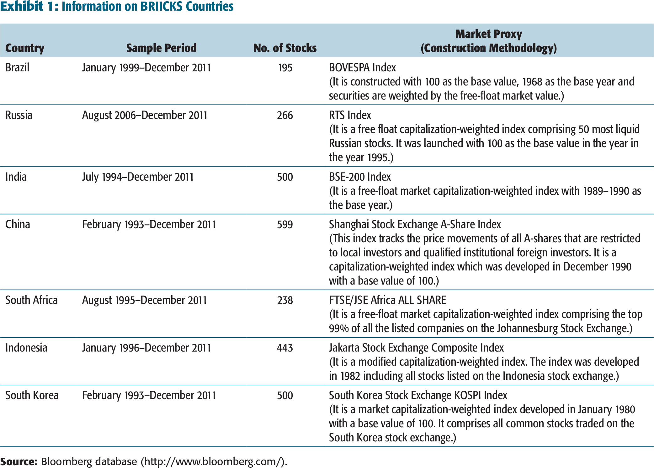
The sample periods are not the same for different markets because of data paucity issues. For the various emerging economies, we have selected actively traded stocks that account for a large part of market capitalization in these markets. In order to facilitate comparison of different economies, the data for all the markets have been given in US dollars. The data comprise of daily adjusted share prices²

Stock price adjustments have been made for dividends, stock splits, and rights issues.

converted to daily percentage returns to make it suitable for further analysis. Market capitalization (price times number of shares outstanding) has been used for construction of size factor and price-to-book value ratio (which is the inverse of book-to-market value ratio) has been used for construction of value factor. The implicit yield on three months US Treasury bill rate has been used as a measure of risk-free rate of return.

SYSTEMATIC VOLATILITY LOADING SORTED PORTFOLIOS

We perform empirical analysis in two parts. The first part involves portfolios sorted on exposure to SV and the second part (covered in the following section) deals with portfolios sorted on UV. The present section deals with the first set of portfolios.

Previous research talks about three measures of SV (or market volatility). The first measure, that is, SVOL, is the market-based variance measure constructed using daily returns on the market index as proposed by French et al. (1987) and Schwert and Seguin (1990). The second measure is RVOL (see Alizadeh, Brandt, & Diebold, 2002), which is a range-based estimate for volatility. The third estimator is VIX, that is, volatility index as suggested by Whaley (2000). VIX is a measure of the amount by which an underlying index is expected to fluctuate, in the near term. Chicago Board Options Exchange VIX is a weighted measure of the implied volatilities for call and put options exhibiting different levels of moneyness. In this article, SVOL has been used to estimate SV. The range-based volatility measure has not been used, as it requires high-frequency intraday data which are not available for the sample countries for a longer time period, which is required for performing such cross-sectional studies. We are also unable to use VIX owing to data paucity problems. VIX is not available for the sample countries over the entire study period. Its construction at our level could introduce estimation biases and make inter-country comparison difficult owing to differences in option price data across markets, for example, nature of options, range of strike prices, varying trading liquidity, length of expiration, etc. Hence, our empirical study is constrained by the choice of SV measure.

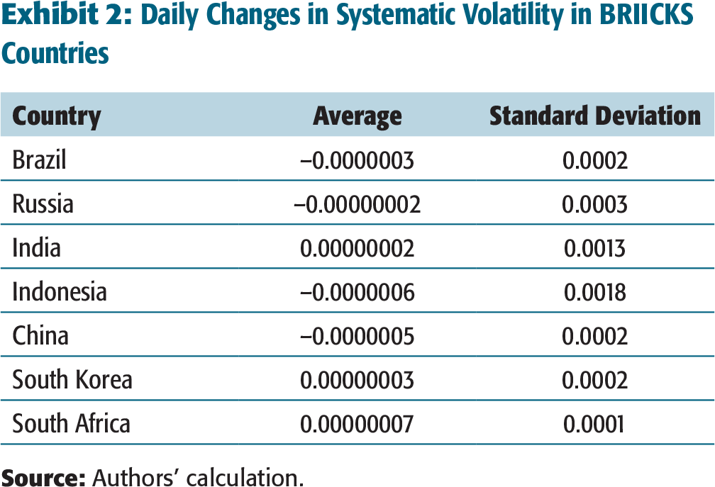
As suggested by French et al. (1987), monthly SVOL (MSVOL) is constructed by taking a sum of squared daily returns over the previous N_t days (N_t = 22 trading days³

Assuming 22 trading days in a month, we use approximately one-month daily returns for estimating SVOL.

in our study) and making an adjustment for first order autocorrelation:

M S V O L = \sum_{i = 1}^{N_{t}} r_{i t}^{2} + 2 \sum_{i = 1}^{N_{t - 1}} r_{i t} r_{i + 1, t}

(1)

where there are N_t daily returns, r_it in a month. As proposed by Ang et al. (2003),⁴

Ang et al. (2003) used standard deviation-based SVOL measure. But we use variance-based SVOL measure for estimation purpose, because we empirically find that cross-sectional differences in returns on portfolios based on standard deviation-based SVOL measure are relatively small. Moreover, later in the study, we sort portfolios on the measure of idiosyncratic risk which is again estimated as unsystematic variance.

we convert monthly SVOL into daily SVOL by dividing MSVOL by N_t, that is, 22 trading⁵

Assuming 22 trading days in a month.

days. We generate time series of daily SVOL on a moving average basis by skipping one day of sample market return. Using daily SVOL, we obtain change in SV as ΔV_t = V_t – V_t-1, where V_t denotes SVOL on day t. Ideally, innovations in volatility involving unexpected changes should have been taken. But due to estimation problems, we employ total change in volatility as a proxy measure for innovations in volatility as in the case of Ang et al. (2003). Mean and standard deviation of our daily changes in SV is given in Exhibit 2. Daily mean is close to zero in all sample countries. The mean standard deviation is again low and ranges from 0.0001 for South Africa to 0.0018 for Indonesia. The daily changes in SV are not auto-correlated for the sample markets.

Exhibit 2:

Daily Changes in Systematic Volatility in BRIICKS Countries

Country	Average	Standard Deviation
Brazil	–0.0000003	0.0002
Russia	–0.00000002	0.0003
India	0.00000002	0.0013
Indonesia	–0.0000006	0.0018
China	–0.0000005	0.0002
South Korea	0.00000003	0.0002
South Africa	0.00000007	0.0001

Source: Authors’ calculation.

The following regression is used to estimate the sensitivity of excess stock return to change in SV:

r_{i t} - r_{f t} = α + β_{1} (r_{m t} - r_{f t}) + β_{2} Δ V_{t} + e_{t}

(2)

where

$(r_{i t} - r_{f t})$ is excess stock return

$(r_{m t} - r_{f t})$ is excess market return

$Δ V_{t} = V_{t} - V_{t - 1}$ gives change in SV.

Equation (2) is estimated for all the sample stocks in each sample country if at least 14 daily return values are available for a given month. Estimating the above regression for the first month gives β₂ values for all the sample stocks. β₂ measures the sensitivity to changes in SV. On the basis of β₂ values, we sort stocks into five portfolios. Portfolio 1 (henceforth referred to as P1) includes high β₂ stocks, that is, stocks with highest exposure to changes in SV. Portfolio 5 (i.e., P5), on the contrary, includes stocks with lowest exposure to changes in SV. For every portfolio, we estimate equally weighted return⁶

Equally weighted portfolios have been preferred, as unsystematic risk diversifies away in their case more quickly (with lower number of securities) than value-weighted portfolios. But it will be interesting to see in future research if empirical results vary when value-weighted portfolios are constructed for systematic as well as UV.

for the second month. Similarly, we estimate β2 values for all sample stocks for the second month, construct five portfolios, and estimate average return on these portfolios for the third month. The procedure continues till we reach the end of the study period.

Empirical Results for Systematic Volatility Loading Portfolios

We construct monthly portfolios on the basis of a stock’s exposure to change in SV. Portfolio 1 (Portfolio 5) consists of stocks with high (low) volatility. Table 1 demonstrates the empirical results for SV loading portfolios. Panel A provides mean portfolio excess returns. It also shows the risk premium estimated as the difference between the returns on P1 and P5 portfolios. Panel B shows the results of CAPM where excess portfolio returns are regressed on the returns for the market factor. Panel C gives Fama–French model results in which the excess portfolio returns are regressed on market, size, and value factors.

The average excess returns of the corner portfolios⁷

P1 and P5, the two extreme portfolios based on given ranking criteria, are termed as corner portfolios in the study.

for the sample countries are shown in Panel A. In both Tables 1 and 2, we report results of the corner portfolios. The focus of the study is on analysing the behaviour of these portfolios since hedge fund and other portfolio managers tend to devise long–short strategy based on corner portfolios and hence have limited or no interest in intermediate portfolios. From an academic point of view, the middle portfolios are generally eliminated, as the corner portfolios shall exhibit the maximum between group variance. Further, in case of cross-country studies, it is a standard practice to report results for only corner portfolios (see Griffin, Ji, & Martin, 2003; Sehgal, Subramaniam, & Deisting, 2014).

Table 1:

Empirical Results for Systematic Volatility Loading Portfolios

Panel :A Unadjusted Portfolio Returns
				Portfolio 1	Portfolio 5	P1–P5
			Brazil	0.0206(2.0574)	0.0361(3.3073)	–0.0155(–8.0309)
			China	0.0172(1.5929)	0.0150(1.4742)	0.0022(0.9723)
			India	0.0131(1.7701)	0.0130(1.6804)	0.0001(0.0853)
			Indonesia	0.0359(2.1350)	0.0263(1.7883)	0.0096(1.9306)
			South Korea	0.0099(1.2215)	0.0135(1.5426)	–0.0035(–2.3053)
			Russia	0.0048(0.3027)	0.0132(0.7789)	–0.0084(–2.7686)
			South Africa	0.0193(3.1441)	0.0157(2.4319)	0.0036(4.6194)
Panel B: CAPM Regression: (r_pt - r_ft) = a + b (r_mt - r_ft)
				A	B	Adjusted R²
Brazil			Portfolio 1	0.0057(1.5629)	0.9439(31.8273)	0.8687
Brazil			Portfolio 5	0.0209(3.9076)	0.9678(22.3035)	0.7644
China			Portfolio 1	0.0096(1.5605)	0.9094(21.1848)	0.6766
China			Portfolio 5	0.0073(1.5450)	0.9218(28.0662)	0.7862
India			Portfolio 1	0.0049(1.3167)	1.1062(25.0414)	0.7524
India			Portfolio 5	0.0043(1.1456)	1.1639(25.7191)	0.7623
Indonesia			Portfolio 1	0.0219(2.2178)	1.4324(19.1340)	0.6565
Indonesia			Portfolio 5	0.0131(1.8505)	1.3591(25.3969)	0.7713
South Korea			Portfolio 1	0.0035(0.7605)	0.9164(21.8169)	0.6786
South Korea			Portfolio 5	0.0069(1.2709)	0.9345(18.9221)	0.6134
Russia			Portfolio 1	0.0016(0.2321)	0.9718(16.1834)	0.8055
Russia			Portfolio 5	0.0100(1.1259)	0.9970(12.9957)	0.7271
South Africa			Portfolio 1	0.0140(3.7617)	0.8537(18.5301)	0.6371
South Africa			Portfolio 5	0.0101(2.5431)	0.8840(17.8666)	0.6200
Panel C: Fama-French Regression: (r_pt - r_ft) = a + b (r_mt - r_ft) + s (SMB_t) + h (LMH_t) + e_t
		A	b	S	h	Adjusted R²
Brazil	Portfolio 1	–	–	–	–	–
Brazil	Portfolio 5	0.0101(1.9388)	0.9452(21.3008)	0.5978(5.9936)	0.2380(1.9376)	0.7900
China	Portfolio 1	–	–	–	–	–
China	Portfolio 5	–	–	–	–	–
India	Portfolio 1	–	–	–	–	–
India	Portfolio 5	–	–	–	–	–
Indonesia	Portfolio 1	0.0007(0.1293)	1.1846(22.5220)	0.3827(4.0414)	0.5347(5.5468)	0.8439
Indonesia	Portfolio 5	–	–	–	–	–
South Korea	Portfolio 1	–	–	–	–	–
South Korea	Portfolio 5	–	–	–	–	–
Russia	Portfolio 1	–	–	–	–	–
Russia	Portfolio 5	–	–	–	–	–
South Africa	Portfolio 1	0.0146(3.2935)	0.9723(16.6472)	0.9473(5.6721)	–0.0919(–0.4452)	0.6777
South Africa	Portfolio 5	0.0056(1.1804)	1.0018(15.9512)	1.0024(5.5814)	0.0954(0.4297)	0.6579

Source: Authors’ calculation.

Note: t-statistics are reported in brackets.

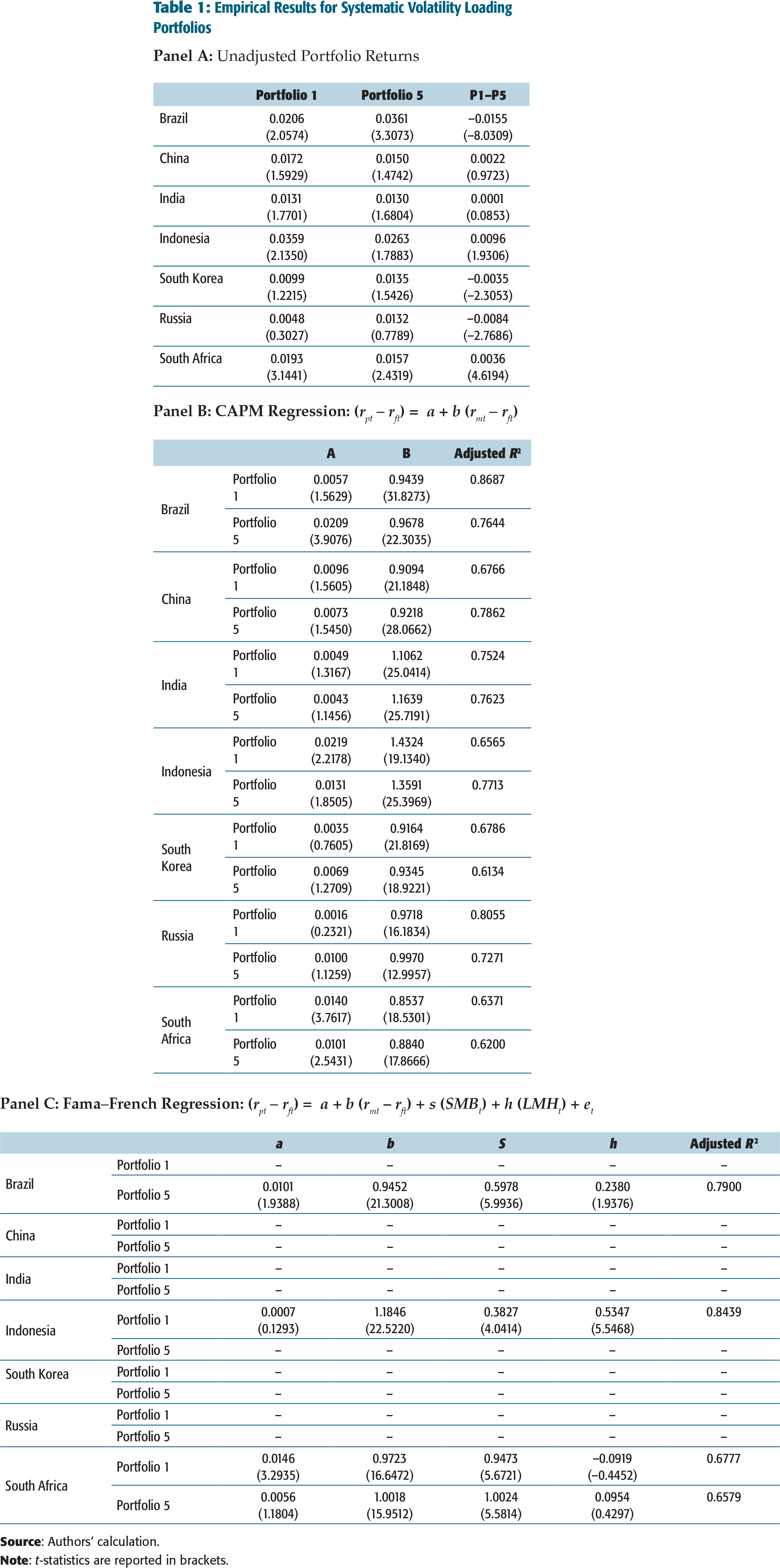
Panel A clearly shows that high SV sensitivity portfolio exhibits low future returns in case of Brazil, South Korea, and Russia. The risk premia estimated as the difference between the returns on P1 and P5 portfolios are statistically, significantly negative for these countries. The findings are consistent with Ang et al. (2006), who obtained similar results for the US market. There can be several economic reasons which explain why the price of risk of changes in market volatility should be negative. Campbell (1993, 1996) and Chen (2002) advocated that investors wanted to hedge against changes in market volatility, because increasing volatility reduced the desirability of investment opportunities. Risk-averse investors prefer stocks that hedge against this risk. Further, higher volatilities are observed generally during market downturns (see Campbell & Hentschel, 1992; French et al., 1987). Bakshi and Kapadia (2003) showed that assets with high sensitivity to market volatility risk provided hedges against market downside risk. The higher demand for these assets increases their price and reduces their average return. Hence, P1 (the high SV loading portfolios) are expected to underperform P5 (the low SV loading portfolios). The results for other sample countries are somewhat puzzling. No significant risk premiums are reported for India⁸

The results reported here for India are different from that in the work of Sehgal et al. (2012). Dollar-based returns have been used here while rupee-denominated returns have been used in the work of Sehgal et al. (2012). Rupee has substantially depreciated vis-à-vis dollar over the study period. Hence, dollar-denominated returns have to be lower than rupee-denominated returns. This is reflected by the empirical results, whereby returns on the corner portfolios have relatively sobered down in this article. Hence, the cross-section of volatility results is much weaker for dollar-denominated returns in the Indian context.

and China. Significantly positive risk premiums are observed for South Africa and Indonesia⁹

Significant at 10 per cent level on a two-tail basis.

which contradict the above-mentioned economic arguments.

Next, we check if there are any risk explanations for the returns on the sample portfolios. Two popular asset pricing models are adopted for this purpose, namely the CAPM and the Fama–French model. Using the CAPM framework, we regress the excess portfolio returns on the excess return for the market factor in the form:

r_{p t} - r_{f t} = a + b (r_{m t} - r_{f t}) + e_{i}

(3)

where

(r_pt – r_ft) is excess return on SV loading sorted portfolio p

(r_mt– r_ft) is excess market return,

a, the intercept, is the measure of abnormal return which is expected to be zero as per CAPM assumption b is the sensitivity coefficient.

Panel B shows that in all the sample countries, both P1 and P5 exhibit almost similar sensitivity to the market factor. CAPM seems to be a poor descriptor of returns on systematic risk loading sorted portfolios with exception of P1 in case of Brazil.

Since CAPM fails to capture the returns on sample portfolios, we regress the portfolio returns on market, size, and value factors using the Fama–French framework as given below:

(r_{p t} - r_{f t}) = a + b (r_{m t} + r_{f t}) + s (S M B_{t}) + h (L M H_{t}) + e_{t}

(4)

where SMB_t and LMH_t are size and value factors, respectively; s and h are sensitivity coefficients while other terms in Equation (4) have the same meaning as in Equation (3). The objective is to verify if the FF model can explain the returns that are missed by CAPM.

The FF model estimation in this article is different in two ways. First, here LMH factor is used in place of HML factor in the Fama–French regression. Therefore, the factor will be interpreted in an inverse manner. Second, we perform a 2*2 size–value partition instead of the 2*3 size–value partition done by Fama and French (1993). The size (SMB) and the value (HML) factors have been constructed as follows. In year t, the sample stocks are divided into two groups, that is, Big (B) and Small (S), on the basis of their market capitalization at the end of December of the year t − 1. Stocks with market capitalization less than the median value are categorized as Small and the remaining are grouped as Big. Similarly, stocks are divided into High (H) and Low (L) groups on the basis of their price-to-book equity ratio. Then, using the intersection of the two size and two P/B groups, we construct four portfolios, namely, S/L, S/H, B/L, and B/H. We then calculate monthly equally weighted returns of these four portfolios from January to December of year t. The FF model uses three independent variables. One is the excess market return which is the return on the market index minus the risk-free rate of return. The second is the size factor (SMB) which is the difference in the average return of the two small size portfolios (S/L, S/H) and the average of the two big size portfolio returns (B/L, B/H):

S M B = (S / L + S / H) / 2 - (B / L + B / H) / 2

(5)

This construction methodology makes SMB factor independent of the value effects. Similarly, the third factor, that is, the value factor (LMH) is constructed in a way that makes it independent of the size effects:

L M H = (S / L + B / L) / 2 - (S / H + B / H) / 2

(6)

In Panel C (Table 1), Fama–French regression results have been reported only for those cases where CAPM fails to explain portfolio return. It clearly shows that FF is able to explain returns on all portfolios except P1 in case of South Africa which seems to be an asset pricing anomaly. Global fund managers can exploit this by developing suitable trading strategy. For example, a long–short strategy for South Africa based on SV loading sorted portfolios is expected to provide a monthly return of 0.9 per cent which is statistically significant at 20 per cent level.

PORTFOLIOS SORTED ON UNSYSTEMATIC VOLATILITY

This section deals with portfolios formed on the basis of UV. UV is calculated using the Fama–French Model. We run the daily FF for every stock i for every month t in the form:

(r_{i t} - r_{f t}) = α + β_{1} (r_{m t} - r_{f t}) + β_{2} (s m b_{t}) + β_{3} (l m h_{t}) + e_{i t}

(7)

where r_it – r_ft is the excess return for stock i on day t, r_mt – r_ft is excess market return on day t and smb_t and lmh_t are size and value proxies, respectively, on day t; α, β₁, β₂, and β₃ are estimated parameters and e_it is the white noise residual term.

The regression (Equation 7) is estimated for the stocks with at least 14 values of daily returns in that month. UV for stock i for month t is obtained by calculating the variance of the daily error terms of that stock i. The stocks are ranked on the basis of their UV in month t and then quintiles are formed. Next, we estimate the equally weighted returns for each of these quintiles for the month t + 1. P5 comprises of one-fifth of the stocks with the lowest UV while P1 contains one-fifth of the stocks with highest UV. Portfolio rebalancing is done at the end of every month till we reach the end of the sample period. Then, we estimate the average unadjusted portfolio returns.

Empirical Results for Portfolios Sorted on Unsystematic Volatility

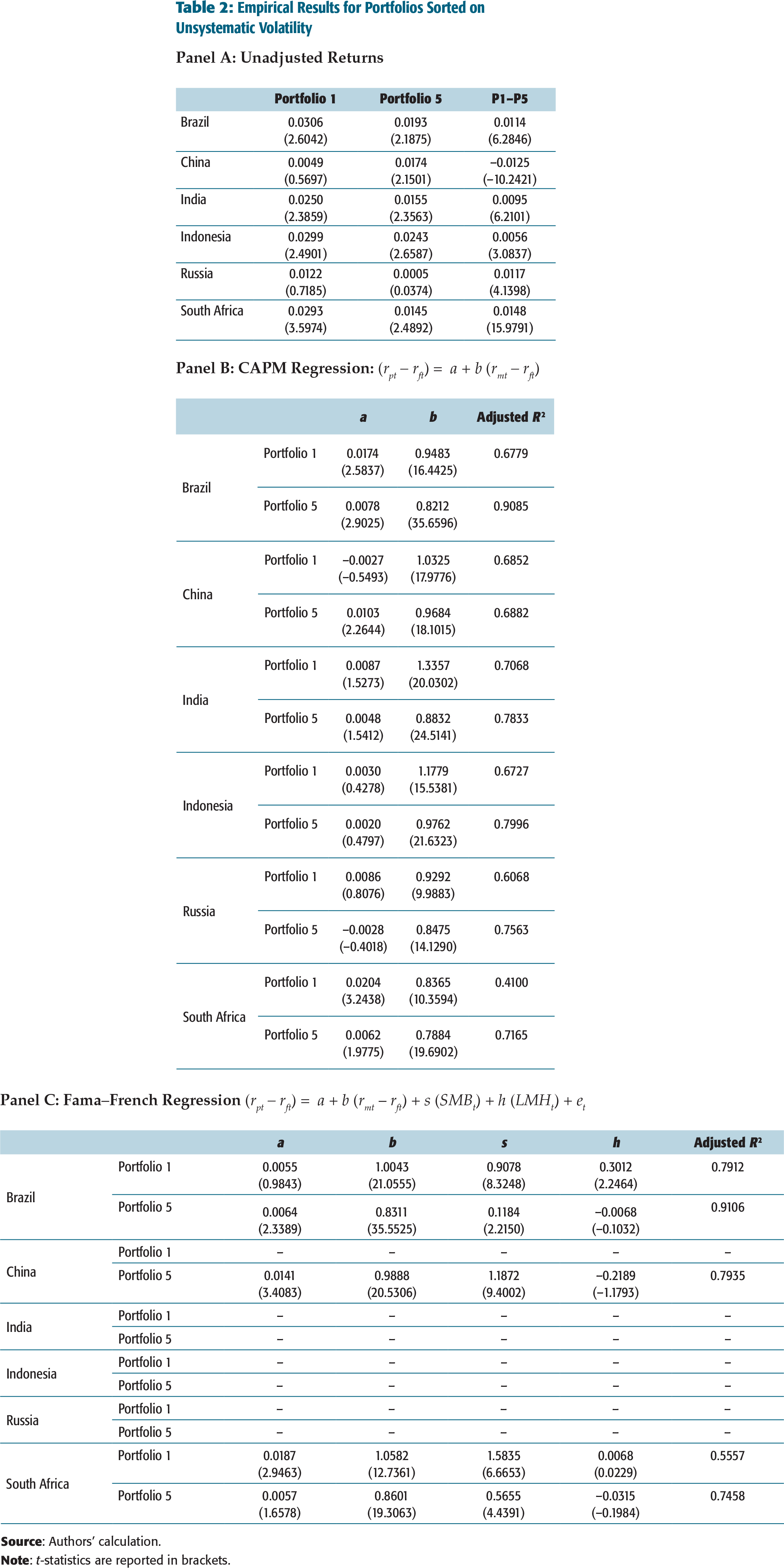
We construct monthly portfolios by sorting the stocks on the basis of UV measured by the variance of the residuals obtained from Fama–French Model. Portfolio 1 (Portfolio 5) comprises high (low) UV stocks. Table 2 demonstrates the empirical results for portfolios sorted on UV. Panel A provides mean portfolio excess returns. It also shows the estimated risk premium, that is, the difference between the returns on P1 and P5 portfolios. Panel B and Panel C give results of CAPM regression and Fama–French regression, respectively.

Panel A of Table 2 clearly shows that high UV portfolios exhibits high returns in all the sample countries¹⁰

UV sorted portfolios have not been constructed for South Korea because of non-availability of daily Fama French Model (FF) factors for several years.

except China. In the Chinese market, the estimated risk premium, that is, the difference between the returns on P1 and P5 is statistically, significantly negative. This is consistent with Ang et al. (2006) for the US market. However, this negative risk premium is inconsistent with the theory which predicts that investors, in most cases, do not hold completely diversified portfolios, and therefore high UV stocks earn high returns to compensate for imperfect diversification. Negative relationship between volatility and returns is often referred to as low volatility anomaly. Possible behavioural explanations for low volatility anomaly can be that investors are irrational and demand high volatility stocks due to their preference for lotteries, the representative bias, or the overconfidence bias (see Baker, Bradley, & Wurgler, 2011). High demand for high volatility stocks increases their price and reduces their expected returns. The remaining sample countries show significantly positive risk premium which is consistent with the imperfect diversification argument.

Next, we regress the returns on UV sorted portfolios on the market factor using the CAPM specification provided in Equation (3).

In Panel B (Table 2), we observe that CAPM is able to explain the returns on the corner portfolios in case of India, Indonesia, Russia, and China (only P1 in Chinese market). The remaining portfolios exhibit significant CAPM alpha values. Therefore, we regress their returns on the FF factors using Equation (4). Panel C (Table 2) reports FF regression results only for those cases where CAPM fails to explain portfolio return. It shows that even FF fails to explain returns on all the portfolios. P5 in case of Brazil and China and P1 in South Africa still exhibit significant alpha values. Testing for long–short strategy for these markets, one finds significant alpha differentials for China (t stats –2.6068) and South Africa (t stats –1.81).¹¹

t statistics of China and South Africa are statistically significant at 5 per cent and 10 per cent, respectively.

Hence, UV sorted portfolios hold promise for developing profitable trading strategies in these markets.

Table 2:

Empirical Results for Portfolios Sorted on Unsystematic Volatility

Panel A: Unadjusted Returns
				Portfolio 1	Portfolio 5	P1–P5
			Brazil	0.0306(2.6042)	0.0193(2.1875)	0.0114(6.2846)
			China	0.0049(0.5697)	0.0174(2.1501)	–0.0125(–10.2421)
			India	0.0250(2.3859)	0.0155(2.3563)	0.0095(6.2101)
			Indonesia	0.0299(2.4901)	0.0243(2.6587)	0.0056(3.0837)
			Russia	0.0122(0.7185)	0.0005(0.0374)	0.0117(4.1398)
			South Africa	0.0293(3.5974)	0.0145(2.4892)	0.0148(15.9791)
Panel B CAPM Regression: (r_pt - r_ft) = a + b (r_mt - r_ft)
				a	b	Adjusted R²
Brazil			Portfolio 1	0.0174(2.5837)	0.9483(16.4425)	0.6779
Brazil			Portfolio 5	0.0078(2.9025)	0.8212(35.6596)	0.9085
China			Portfolio 1	–0.0027(–0.5493)	1.0325(17.9776)	0.6852
China			Portfolio 5	0.0103(2.2644)	0.9684(18.1015)	0.6882
India			Portfolio 1	0.0087(1.5273)	1.3357(20.0302)	0.7068
India			Portfolio 5	0.0048(1.5412)	0.8832(24.5141)	0.7833
Indonesia			Portfolio 1	0.0030(0.4278)	1.1779(15.5381)	0.6727
Indonesia			Portfolio 5	0.0020(0.4797)	0.9762(21.6323)	0.7996
Russia			Portfolio 1	0.0086(0.8076)	0.9292(9.9883)	0.6068
Russia			Portfolio 5	–0.0028(–0.4018)	0.8475(14.1290)	0.7563
South Africa			Portfolio 1	0.0204(3.2438)	0.8365(10.3594)	0.4100
South Africa			Portfolio 5	0.0062(1.9775)	0.7884(19.6902)	0.7165
Panel C: Fam –French Regression (r_pt - r_ft) = a + b (r_mt - r_ft) + s (SMB_t) + h (LMH_t) + e_t
		a	B	s	h	Adjusted R2
Brazil	Portfolio 1	0.0055(0.9843)	1.0043(21.0555)	0.9078(8.3248)	0.3012(2.2464)	0.7912
Brazil	Portfolio 5	0.0064(2.3389)	0.8311(35.5525)	0.1184(2.2150)	–0.0068(–0.1032)	0.9106
China	Portfolio 1	–	–	–	–	–
China	Portfolio 5	0.0141(3.4083)	0.9888(20.5306)	1.1872(9.4002)	–0.2189(–1.1793)	0.7935
India	Portfolio 1	–	–	–	–	–
India	Portfolio 5	–	–	–	–	–
Indonesia	Portfolio 1	–	–	–	–	–
Indonesia	Portfolio 5	–	–	–	–	–
Russia	Portfolio 1	–	–	–	–	–
Russia	Portfolio 5	–	–	–	–	–
South Africa	Portfolio 1	0.0187(2.9463)	1.0582(12.7361)	1.5835(6.6653)	0.0068(0.0229)	0.5557
South Africa	Portfolio 5	0.0057(1.6578)	0.8601(19.3063)	0.5655(4.4391)	–0.0315(–0.1984)	0.7458

Source: Authors’ calculation.

Note: t-statistics are reported in brackets

SUMMARY AND CONCLUSIONS

Cross-sectional volatility measures dispersion of security returns at a particular point of time. It has received very little focus in research. This article studies the cross-section of volatility in the context of BRIICKS economies, namely Brazil, Russia, India, Indonesia, China, South Korea, and South Africa. The analysis is carried out in two parts. The first part deals with SV, that is, cross-sectional variation of stock returns owing to their exposure to market volatility measure. Market volatility measure used is the one suggested by French et al. (1987). The second part deals with UV measured by the residual variance of stocks in a given period by using the error terms obtained from Fama–French (1993) model.

We find that high SV portfolios exhibit low returns in case of Brazil, South Korea, and Russia. The risk premium is found to be statistically, significantly negative for these countries. This finding is consistent with Ang et al. (2006) and is indicative of the hedging motive of investors in these markets. Results for other sample countries are somewhat puzzling. No significant risk premiums are reported for India and China. Significantly positive risk premiums are observed for South Africa and Indonesia.¹²

Significant at 10 per cent level on a two-tail basis.

Further, CAPM seems to be a poor descriptor of returns on systematic risk loading sorted portfolios while FF is able to explain returns on all portfolios except high SV loading portfolio (i.e., P1) in case of South Africa which seems to be an asset pricing anomaly.

We further find that high UV portfolios exhibit higher returns vis-à-vis low UV portfolios in all the sample countries except China. In the Chinese market, statistically, the estimated risk premium is significantly negative. This negative risk premium is inconsistent with the theory which predicts that investors demand risk compensation for imperfect diversification. The remaining sample countries show significantly positive risk premium which is in conformity with the finance theory. CAPM does not seem to be a suitable descriptor for returns on UV sorted portfolios. The FF model does a better job but still fails to explain the returns on high UV sorted portfolio in case of Brazil and China and low UV sorted portfolio in South Africa.

The findings of this study are relevant for global fund managers who plan to develop emerging market strategies for asset allocation. On an overall basis, emerging markets seem to be efficient with regard to cross-sectional volatility-based information with an exception of South Africa and to some extent China. From an academic point of view, the FF model seems to be a better asset pricing tool compared to CAPM for the pricing of cross-sectional volatility sorted portfolios. The study contributes to portfolio management as well as market efficiency literature for emerging economies.

References

Adrian

Rosenberg

(2008). Stock returns and volatility: Pricing the short-run and long-run components of market risk. Journal of Finance , 63(6), 2997–3030.

Alizadeh

Brandt

Diebold

F. X.

(2002). Range-based estimation of stochastic volatility models. Journal of Finance , 57(3), 1047–1091.

Ang

Hodrick

R. J.

Xing

Zhang

(2003). The cross-section of volatility and expected returns. Retrieved 21 March 2015, from http://www.ruf.rice.edu/~yxing/vol.pdf

Ang

Hodrick

R. J.

Xing

Zhang

(2006). The cross-section of volatility and expected returns. The Journal of Finance , 61(1), 259–299.

Baker

Brendan

Jeffrey

(2011). Benchmarks as limits to arbitrage: Understanding the low volatility anomaly. Financial Analysts Journal , 67(1), 1–15.

Bakshi

Kapadia

(2003). Delta-hedged gains and the negative market volatility risk premium. Review of Financial Studies , 16(2), 527–566.

Banz

R. W.

(1981). The relationship between return and market value of common stocks. Journal of Financial Economics , 9(1), 3–18.

Basu

(1983). The relationship between earnings yield, market value, and return for NYSE common stocks: Further evidence. Journal of Financial Economics , 12(1), 129–156.

Benzoni

(2002). Pricing options under stochastic volatility: An empirical investigation (Working paper). University of Minnesota. Retrieved 15 January, 2015 from https://sites.google.com/site/lbenzonifrbchi/SV_07_02.PDF

10.

Bhandari

L. C.

(1988). Debt/equity ratio and expected common stock returns: Empirical evidence. Journal of Finance , 43(2), 507–528.

11.

Black

(1972). Capital market equilibrium with restricted borrowing. Journal of Business , 45(3), 444–455.

12.

Campbell

J. Y.

(1993). Intertemporal asset pricing without consumption data. American Economic Review , 83(3), 487–512.

13.

Campbell

J. Y.

(1996). Understanding risk and return. Journal of Political Economy , 104(2), 298–345.

14.

Campbell

J. Y.

Hentschel

(1992). No news is good news: An asymmetric model of changing volatility in stock returns. Journal of Financial Economics , 31(3), 281–318.

15.

Campbell

J. Y.

Lettau

Malkiel

B. G.

(2001). Have individual stocks become more volatile? An empirical exploration of idiosyncratic risk. Journal of Finance , 56(1), 1–44.

16.

Chen

(2002, May). Intertemporal, CAPM and the cross-section of stock returns. Berlin Meetings Discussion Paper . Retrieved 12 May, 2016 from http://papers.ssrn.com/sol3/papers.cfm?abstract_id=301918

17.

Chiang

T. C.

Doong

S. C.

(2001). Empirical analysis of stock returns and volatility: Evidence from seven Asian stock markets based on TAR-GARCH model. Review of Quantitative Finance and Accounting , 17(3), 301–318.

18.

Connolly

Stivers

(2006). Information content and other characteristics of daily cross-firm stock volatility. Journal of Empirical Finance , 13(1), 79–112.

19.

Cutler

D. M.

(1989). Stock market volatility, cross section volatility and stock returns (Working paper). MIT.

20.

De Bondt

W.F.

Thaler

(1985). Do the stock markets overreact? Journal of Finance , 40(3), 793–805.

21.

De Bondt

W.F.

Thaler

(1987). Further evidence of investor overreaction and stock market seasonality. Journal of Finance , 42(3), 557–581.

22.

De Santis

Imrohoroglu

(1997). Stock returns and volatility in emerging financial markets. Journal of International Money and Finance , 16(4), 561–579.

23.

Dimitrios

Theodore

(2011). The relationship between stock returns and volatility in the seventeen largest international stock markets: A semi-parametric approach. Modern Economy , 2(1), 1–8.

24.

Ederington

L. H.

Guan

(2005). Forecasting volatility. Journal of Futures Markets , 25(5), 465–490.

25.

Fama

E. F.

French

K. R.

(1993). Common risk factors in the returns on stocks and bonds. Journal of Financial Economics , 33(1), 3–56.

26.

French

K. R.

Schwert

G. W.

Stambaugh

R. F.

(1987). Expected stock returns and volatility. Journal of Financial Economics , 19(1), 3–29.

27.

Glosten

L. R.

Jagannathan

Runkle

D.E.

(1993). On the relation between the expected value and the volatility of the nominal excess return on stocks. Journal of Finance , 48(5), 1779–1801.

28.

Griffin

J. M.

Martin.

J.S.

(2003). Momentum investing and business cycle risk: Evidence from pole to pole. Journal of Finance , 58(6), 2515–2547.

29.

Hull

White

(1987). The pricing of options on assets with stochastic volatilities. Journal of Finance , 42(2), 281–300.

30.

Hwang

Satchell

(2001). GARCH model with cross-sectional volatility: GARCHX models (Working paper). City University Business School. Retrieved 12 May, 2016 from http://www2.warwick.ac.uk/fac/soc/wbs/subjects/finance/research/wpaperseries/2001/soosung_hwang_and_satchell.pdf

31.

Jegadeesh

Titman

(1993). Returns to buying winners and selling losers: Implications for stock market efficiency. Journal of Finance , 48(1), 65–92.

32.

Lee

C. F.

Chen

Rui

(2001). Stock returns and volatility on China’s stock markets. Journal of Financial Research , 24(4), 523–543.

33.

Lintner

(1965). The valuation of risk assets and the selection of risky investments in stock portfolios and capital budgets. Review of Economics and Statistics , 47(1), 13–37.

34.

Merton

R. C.

(1973). An intertemporal capital asset pricing model. Econometrica , 41(5), 867–887.

35.

Rahman

M. A.

(2007). The information content of cross-sectional volatility for future market volatility: Evidence from Australian equity returns. Frontiers in Finance and Economics , 4(1), 91–124.

36.

Rosenberg

Reid

Lanstein

(1985). Persuasive evidence of market inefficiency. Journal of Portfolio Management , 11(1), 9–17.

37.

Schwert

G. W.

(1989). Why does stock market volatility change over time? Journal of Finance , 44(5), 1115–1154.

38.

Schwert

G. W.

Seguin

P. J.

(1990). Heteroskedasticity in stock returns. Journal of Finance , 45(4), 1129–1155.

39.

Sehgal

Garg

Deisting

(2012). Relationship between cross-sectional volatility and stock returns: Evidence from India. Investment Management and Financial Innovations , 9(2), 90–99.

40.

Sehgal

Subramaniam

Deisting

(2014). Tests of equity market anomalies for select emerging markets. The International Journal of Business and Finance Research , 8(3), 27–46.

41.

Sehgal

Vijayakumar

(2008). Determinants of implied volatility function on the NIFTY index options market: Evidence from India. Asian Academy of Management Journal of Accounting and Finance, 4(1), 45–69.

42.

Sharpe

W. F.

(1964). Capital asset prices: A theory of market equilibrium under conditions of risk. Journal of Finance , 19(3), 425–442.

43.

Shin

(2005). Stock returns and volatility in emerging stock markets. International Journal of Business and Economics , 4(1), 31–43.

44.

Stattman

(1980). Book values and stock returns. The Chicago MBA: Journal of Selected Papers , 4, 25–45.

45.

Whaley

(2000). The investor fear gauge. Journal of Portfolio Management , 26(3), 12–17.

46.

Wiggins

J. B.

(1987). Option values under stochastic volatilities. Journal of Financial Economics , 19(2), 351–372.

Cross-sectional Volatility and Stock Returns: Evidence for Emerging Markets

Abstract

Executive Summary

Keywords

LITERATURE REVIEW

DATA

Information on BRIICKS Countries

SYSTEMATIC VOLATILITY LOADING SORTED PORTFOLIOS

Daily Changes in Systematic Volatility in BRIICKS Countries

Empirical Results for Systematic Volatility Loading Portfolios

Empirical Results for Systematic Volatility Loading Portfolios

PORTFOLIOS SORTED ON UNSYSTEMATIC VOLATILITY

Empirical Results for Portfolios Sorted on Unsystematic Volatility

Empirical Results for Portfolios Sorted on Unsystematic Volatility

SUMMARY AND CONCLUSIONS

References