Sage Journals: Discover world-class research

Abstract

Interregional electricity trade in the United States reduces total energy costs, but falls short of maximizing the economic potential of existing transmission infrastructure. This analysis of thirty-two U.S. electricity system interfaces crossing grid or market seams finds an average achieved cost savings of at least $1,226 million per year. This positive impact is offset by an average annual cost of uneconomic interchange of $551 million. Additional value of at least $238 million per year could be enabled by increasing utilization. Notably, uneconomic flows and low utilization rates can persist even when the price spread between regions is large. These conclusions are derived from historical (2014–2023) data on the magnitude and direction of interregional price spreads, the magnitude and direction of net energy transfers, and how these variables coincide, but do not account for all system constraints. These findings motivate the development and deployment of solutions that improve interregional transmission operations, in parallel with robust transmission infrastructure planning.

JEL Classification: Q40 Energy: General

Keywords

electricity transmission grid seams operational efficiency

1. Introduction

Improving coordination between neighboring power systems can improve system reliability and affordability and has been a noted goal for multiple decades. For example, in 2006, European countries incrementally began coupling their electricity markets to better utilize cross-border transmission lines. In the eastern United States, market monitors began documenting trade inefficiencies between adjacent markets in 2004 and, despite reforms in the intervening years, still find pervasive issues in 2024 and recommend further reforms. Although not a new issue, interregional transmission operations have recently attracted greater attention (Alagappan et al. 2024; Pfeifenberger, DeLosa, et al. 2023; Simeone and Rose 2024). Three reasons motivate this renewed focus: First, rising retail electricity prices (U.S. Bureau of Labor Statistics 2024) lead to efficiency reviews of many asset classes and operational procedures. Second, analysis of outages caused by recent winter storms and heat waves has highlighted that interregional coordination can contribute to balancing the electrical grid during extreme weather events (Goggin and Zimmerman 2023; Panteli and Mancarella 2015). Third, least-cost models of future U.S. power systems forecast a substantial increase in transmission infrastructure to serve new demand (e.g., data centers, manufacturing), facilitate integration of renewable generation (Bloom et al. 2016), and to support emission reduction goals (Denholm et al. 2022; Larson et al. 2021; U.S. Department of Energy 2023), where applicable. The prospect of transmission investment motivates assessment of the efficacy of existing transmission infrastructure. Given the growing importance of interregional coordination, a comprehensive, nationwide assessment of operational efficiency is needed, and is a key goal of this paper. Here we review the past decade of U.S. cross-market electricity flows, document the value of those flows, and analyze missed opportunities and inefficiencies in trade.

Cross-region coordination is managed differently from within-region system operation. Within a region, the system operator – a Regional Transmission Organization (RTO), Independent System Operator (ISO), or vertically-integrated utility – dispatches generators and demand-side resources to reliably meet the system’s electrical loads in a cost-effective way that is feasible given the constraints of those resources and the transmission facilities. RTOs and ISOs dispatch generation in the order of lowest price offers in a multi-unit auction, while vertically-integrated utilities dispatch generation according to a least-cost optimization procedure. A large literature exists studying the efficiency in both forms of internal transmission system operation (Cicala 2022; Davis and Wolfram 2012; Fabrizio et al. 2007).

Transmission infrastructure operation across market seams, however, requires intentional coordination and management among multiple parties to be used safely, reliably, and economically. Standards issued by the North American Electric Reliability Corporation (NERC) and North American Energy Standards Board (NAESB) – specifically NERC INT-001, 003, and 004-1 and NAESB WEQ-004 – define procedures for coordinating bilateral interchange transactions between the source and sink balancing authorities and the purchasing-selling entity. The procedures focus on ensuring system reliability and enabling market-based operations. Designing market mechanisms to facilitate economically efficient trade across interfaces is not within the scope of these standards, thus practices for allocating transmission rights and scheduling interchange vary by region.

In this paper, we focus on the economics of market seams, presenting signals of inefficient use of interregional transmission infrastructure and characterizing the economic opportunity available through more efficient use. For each of thirty-two transmission interfaces, we document the energy transfers that occurred at an hourly resolution: what direction power flowed and how such hourly exchange is aligned with real-time energy prices. Using this information we estimate that these thirty-two interfaces delivered, in aggregate, average economic gains of $1.23 billion per year by transferring energy from lower to higher-priced regions, but almost 50 percent of these gains are lost due to inefficiencies. These results provide a baseline for understanding cross-region energy trade today and highlight opportunities to increase efficiency within the electricity system by improving the use of interregional transmission infrastructure.

This work contributes to a growing literature on the value of transmission in enabling geographic integration in electricity markets. Transmission facilitates market integration across regions by enabling trade, and prior work has documented the effects of transmission constraints on price spreads and generation costs within (Davis and Hausman 2016; LaRiviere and Lyu 2022) and across regions (Cicala 2022; Gonzales et al. 2023; Hausman 2024). This paper extends that literature in two ways. First, our power flow and wholesale price data-driven methodology contrasts with prior studies that estimate regional supply curves using unit-level generation data to analyze a single interface. Our approach, while not appropriate for modeling changes in generation at the plant level, reveals substantial heterogeneity in the degree of regional market integration and enables assessments of potential drivers of efficient interregional trade. Second, our analysis of interregional trade is not limited to physical capacity constraints, but it holistically considers any physical, economic, and structural trading barriers that were present. As a result, we document new patterns of efficient trade, uneconomic flow, and low levels of transmission utilization that are unlikely to be explained by physical constraints alone.

This paper also contributes to a broad, empirical literature on strategic interactions and economic efficiency within electricity markets. Previous work has analyzed how market-based dispatch mechanisms can increase economic efficiency in electricity markets (Cicala 2022; Mansur and White 2012), but that opportunities for inefficiency remain, particularly when sellers exercise market power to raise wholesale prices (Borenstein et al. 2002; Bushnell et al. 2008; Hortaçsu and Puller 2008; Ryan 2021; Wolak 2015). Electricity market monitor reports have long documented inefficiencies at market seams (ISO New England Inc. Internal Market Monitor 2023; Monitoring Analytics, LLC 2023; Potomac Economics 2023a, 2023b, 2023c). However, the data analyzed and analytical approach taken within these market monitor reports varies by region and by interface assessed, making it difficult to assess the scope of the inefficiency at a national scale.

Our study advances this discussion by developing a unified, well-documented methodology to quantify seams-related inefficiencies. First, we find evidence that a significant share of interregional power flow is uneconomic; importers and exporters submit bids or schedules that do not ultimately lead to cost-minimizing trades across regions. Our findings parallel Hortaçsu and Puller (2008) and Hortaçsu et al. (2019), who found that bidding behavior in the Texas real-time electricity market deviated from profit-maximizing benchmarks. Second, we document low interface utilization, even when price spreads are large, consistent with existing literature that finds opportunities exist to enhance market integration using existing transmission capacity. Pineau and Lefebvre (2009) similarly identify underused interregional transmission connected to Quebec during 2006 to 2008, and Ovaere et al. (2023) found that adopting flow-based market coupling in Central Western Europe increased cross-border exchange volumes and price convergence during 2015 to 2017.

Lastly, we complement the literature on capacity expansion models that optimize transmission build-out and operation (Ringkjøb et al. 2018). This vast literature provides important direction to policy makers and system planners on the structure of a cost-optimized electricity systems, but it does not consider empirical data on actual transmission operation (Brown and Botterud 2021; Frew et al. 2016; MacDonald et al. 2016; Mai et al. 2014). Such models are often idealized representations of the electricity system, and their designs either omit or only roughly integrate market seams inefficiencies. While in some cases this is appropriate for the aims of the study, in other cases, such inefficiencies are not reflected because they are too hard to model or they are not well known because there is limited observational research into the operation of existing interregional transmission interfaces – a gap we aim to fill in this paper.

2. Geographic Scope and Data

Interfaces are boundaries between power systems at which balancing authorities record electricity flows. This paper covers thirty-two interfaces reported by the seven regional transmission organizations in the United States (California ISO –“CAISO,” Electric Reliability Council of Texas –“ERCOT,” PJM Interconnection –“PJM,” Midcontinent ISO –“MISO,” New England ISO “ISO-NE,” New York ISO –“NYISO,” and the Southwest Power Pool –“SPP”), including select interconnections with Canada and market-to-non-market interfaces with neighboring balancing areas, as depicted in Figure 1. Because of this broad scope, our insights are not limited to specific market conditions: the areas connected to these interfaces are diverse in their resource mixes, market characteristics, and regulatory institutions. An interface may aggregate flows across one or more physical transmission lines; for example, the “NYISO-PJM” interface represents flows across twenty five transmission lines that run between the PJM and New York ISO footprints, while the “NYISO-PJM Neptune” interface reports flows from a single direct-current (DC) line connecting the two regions. Combined, these thirty-two interfaces represent approximately 50 GW of transfer capability, a majority¹ of transfer capability between FERC Order No. 1000 planning regions in the U.S. plus that between the U.S. and Ontario and Manitoba. An interface within this geographic scope and not included here is excluded for one of the following reasons: (1) It is a non-market-to-non-market interface, which lack the necessary market structures and data transparency for this analysis framework; (2) It had information or data gaps preventing analysis; (3) It is a CAISO interface that was deprioritized due to the infeasibility of analyzing all fifty CAISO-reported interfaces.

Figure 1.

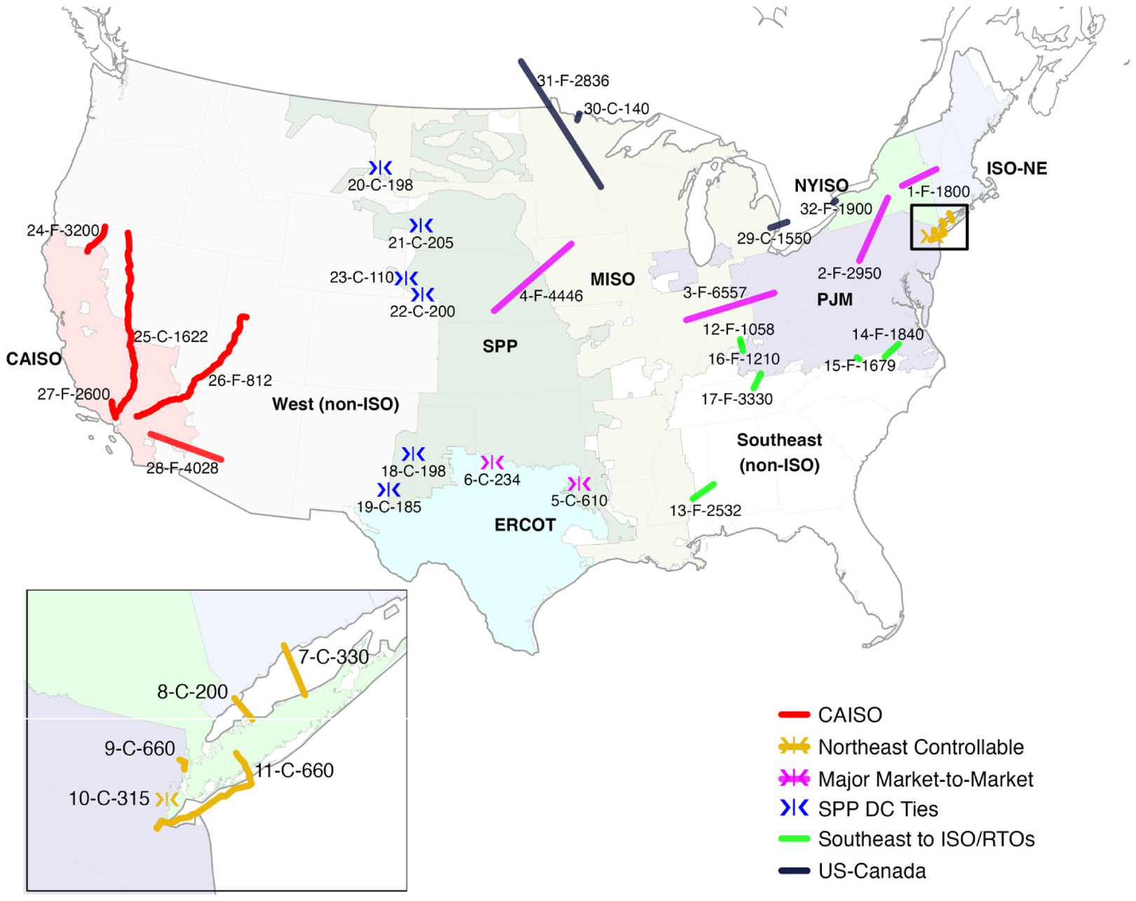
Map representing the thirty-two analyzed interfaces labeled as “#– controllability indicator – max capacity in MW” where # corresponds to Table 3 and the controllability indicator is F for free-flowing and C for controllable interfaces. Back-to-back converter station interfaces and the Linden variable frequency transformer are represented by the > | < symbol. The remaining interfaces are shown as either a specific transmission line or a straight line between the two relevant balancing authorities.

We build a panel data set on interregional transmission in the United States, collecting historical information on net electricity flows across interfaces, electricity market prices, and system marginal costs. These data allow us to quantify price differences, transmission capacity utilization, and the direction of flow across interfaces. This information is publicly available through a combination of system operator reports and data portals and Federal Energy Regulatory Commission (FERC) filings. However, we purchased these data from a commercial vendor to expedite data collection and standardization; the product is called Velocity Suite, by Hitachi. Where possible, we analyzed ten years of data covering 2014 to 2023, however for some interfaces the data sample starts as recently as June 2021. All data reflects observed system outcomes; forecasted data is not used. Table 1 details the dataset construction and timeline analyzed for each interface.

Table 1.

Summary of Data Construction.

Interface name	BA reporting flow	Transmission path	Flow schedule	Price node _a	Price node _b	Imputed limit	Start of sample	End of sample
NYISO-NE ISO	New England ISO	NY Northern AC to ISONE	Scheduled	N.E._GEN_SANDY PD	.I.ROSETON 345 1		2014-01-01	2023-12-31
NYISO-PJM	PJM ISO	NYISO to PJM	Scheduled	PJM	NYIS		2014-01-01	2023-12-31
PJM-MISO	Midcontinent ISO	PJM to MISO	Scheduled	MISO*	PJMC	Y	2014-01-01	2023-12-31
SPP-ERCOT E	SPP	ERCOT East DC Tie to SPP	Actual	ERCOTE	DC_E	Y	2014-02-28	2023-12-31
SPP-ERCOT N	SPP	ERCOT North DC Tie to SPP	Actual	ERCOTN	DC_N	Y	2014-04-01	2023-12-31
SPP-MISO	Midcontinent ISO	SWPP to MISO	Scheduled	MISO	SWPP	Y	2014-03-01	2023-12-31
NYISO-NE CSC	New England ISO	Cross Sound Cable to ISONE	Scheduled	NPX_GEN_CSC	.I.SHOREHAM138 99		2014-01-01	2023-12-31
NYISO-NE Northport	New England ISO	NY NNC to ISONE	Scheduled	NPX_GEN_1385_PROXY	.I.NRTHPORT138 5		2014-01-01	2023-12-31
NYISO-PJM Hudson	PJM ISO	Hudson Line to PJM	Scheduled	PJM_GEN_HTP_PROXY	HUDSONTP		2014-01-01	2023-12-31
NYISO-PJM Linden	PJM ISO	Linden VFT to PJM	Scheduled	PJM_GEN_VFT_PROXY	LINDENVFT		2014-01-01	2023-12-31
NYISO-PJM Neptune	PJM ISO	Neptune Line to PJM	Scheduled	PJM_GEN_NEPTUNE_PROXY	NEPTUNE		2014-01-01	2023-12-31
MISO-LGEE	Midcontinent ISO	LGEE to MISO	Scheduled	LGEE	LG&E & KU Services Co^	Y	2021-01-01	2023-12-31
MISO-SOCO	Midcontinent ISO	Southern Co to MISO	Scheduled	SOCO	Southern Co Services Inc^	Y	2014-01-01	2023-12-31
PJM-CPLE	PJM ISO	CPLE to PJM	Scheduled	SOUTH	Duke Energy Progress East^	Y	2021-06-01	2023-12-31
PJM-Duke	PJM ISO	Duke to PJM	Scheduled	SOUTH	Duke Energy Carolinas LLC^	Y	2021-06-01	2023-12-31
PJM-LGE	PJM ISO	LGE to PJM	Scheduled	SOUTH	LG&E & KU Services Co^	Y	2021-06-01	2023-12-31
PJM-TVA	PJM ISO	TVA to PJM	Scheduled	SOUTH	Tennessee Valley Authority^	Y	2021-06-01	2023-12-31
SPP-WECC Blackwater	SPP	Blackwater DC Tie to SPP	Actual	BLKW	Public Service Co of New Mexico^	Y	2014-02-28	2023-12-31
SPP-WECC Eddy	SPP	EDDY DC Tie to SPP	Actual	EDDY	El Paso Electric^	Y	2014-02-28	2023-12-31
SPP-WECC Miles	SPP	Miles City West DC Tie to SPP	Actual	MCWEST	Northwestern Energy^	Y	2021-01-01	2023-12-31
SPP-WECC Rapid City	SPP	Rapid City East DC Tie to SPP	Actual	RCEAST	WACM.BHP.LANGE	Y	2021-01-05	2023-12-31
SPP-WECC Sidney	SPP	Sydney DC Tie to SPP	Actual	SCSE	WACM.LAPM.BIGTHOMPSON	Y	2021-01-05	2023-12-31
SPP-WECC Stegall	SPP	Stegall DC Tie to SPP	Actual	SGE	WACM.BEPM.LRS2	Y	2021-01-05	2023-09-30
CAISO-BPA Malin	California ISO	MALIN500	Scheduled	TH_NP15_GEN-APND	MALIN_5_N101		2014-05-21	2023-12-31
CAISO-BPA Nob	California ISO	NOB_ITC	Scheduled	DLAP_SCE-APND	SYLMARDC_2_N501		2014-05-21	2023-12-31
CAISO-LDWP Ipputah	California ISO	IPPUTAH_ITC	Scheduled	TH_SP15_GEN-APND	INTERMT_3_N506		2014-08-30	2023-12-31
CAISO-LDWP Sylmar	California ISO	SYLMAR-AC_ITC	Scheduled	DLAP_SCE-APND	SYLMARLA_2_N501		2014-05-21	2023-12-31
CAISO-SRP Palo Verde	California ISO	PALOVRDE_ITC	Scheduled	TH_SP15_GEN-APND	PALOVRDE_5_N101		2014-05-21	2023-12-31
MISO MI-Ontario	IESO (Ontario)	Michigan to Ontario	Scheduled	ONT	Michigan		2014-01-01	2023-12-31
MISO MN-Ontario	IESO (Ontario)	Minnesota to Ontario	Scheduled	ONT_W	Minnesota		2014-01-01	2023-12-31
MISO-MHEB	Midcontinent ISO	MHEB to MISO	Scheduled	MINN.HUB	MHEB	Y	2014-01-01	2023-12-31
NYISO-Ontario	IESO (Ontario)	New York to Ontario	Scheduled	O H	New-York		2014-01-01	2023-12-31

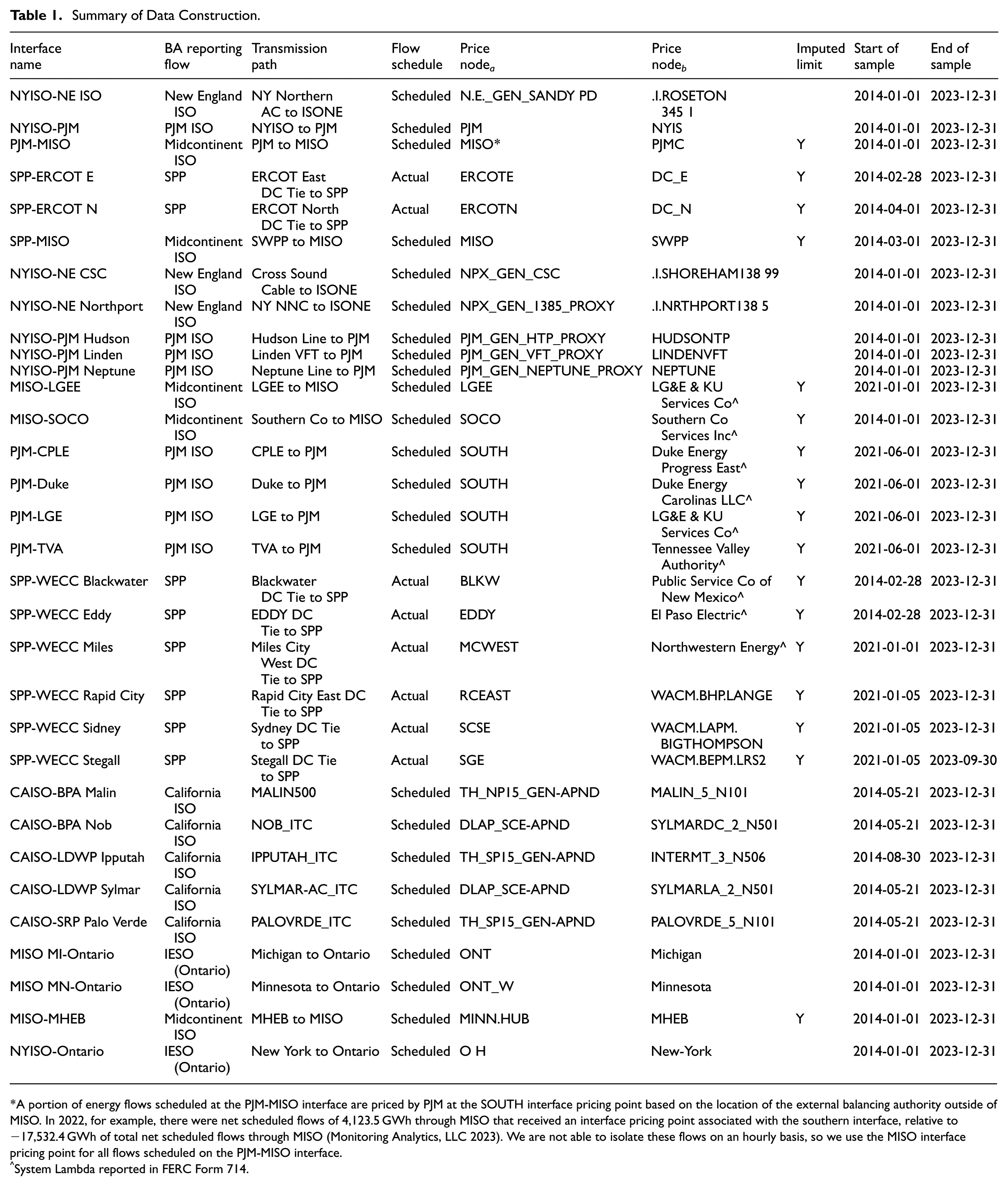
A portion of energy flows scheduled at the PJM-MISO interface are priced by PJM at the SOUTH interface pricing point based on the location of the external balancing authority outside of MISO. In 2022, for example, there were net scheduled flows of 4,123.5 GWh through MISO that received an interface pricing point associated with the southern interface, relative to −17,532.4 GWh of total net scheduled flows through MISO (Monitoring Analytics, LLC 2023). We are not able to isolate these flows on an hourly basis, so we use the MISO interface pricing point for all flows scheduled on the PJM-MISO interface.

System Lambda reported in FERC Form 714.

2.1. Interface Classification

The thirty-two interfaces studied here are not homogeneous. One important difference is whether power flow on the interface is “controllable” or “free-flowing.” The controllable interfaces in this paper are either a variable frequency transformer, a DC tie (either a DC line or a back-to-back converter station), or an AC line paired with phase angle regulating transformers. These interfaces are distinct from the majority of the transmission system that consists of meshed alternating current (AC) networks. On such networks, the path of power flow cannot be prescribed, because electricity flows across transmission facilities according to Kirchoff’s Laws based on the power consumption of loads and the voltage magnitude and real power injection established by generators. This feature of AC networks can limit the ability for interregional transmission to create gains from trade, as power can follow an unintended path that does not correspond to the cost-minimizing route. (See Garg 2015 for a discussion on how loop flows have created conflicts between interregional transmission operators.) Because controllable interfaces can reliably dispatch capacity to and from specified areas, they may have greater ability to optimize interregional flows (Pfeifenberger, Bai, and Levitt 2023).

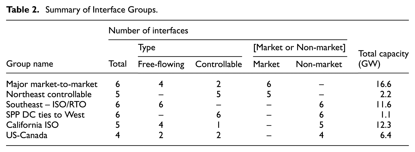
To facilitate high-level comparisons between different categories of interfaces and individual comparisons of an interface to its peers, we have partitioned the interfaces into groups that share similar geographic, physical, and economic characteristics. The groups are: Major market-to-market, Northeast controllable, Southeast ISO/RTO interfaces, Southwest Power Pool DC ties to West, California ISO, and US-Canada. Table 2 summarizes the composition of each group while Table 3 and Figure 1 label each interface according to their peer group and whether they are free-flowing or controllable. The SPP DC ties to West group consists of six back-to-back converter stations linking the asynchronous eastern and western interconnections. These interfaces utilize different technology and operating procedures than the meshed AC networks consisting of many transmission lines that span from utilities in the Southeast to their neighboring ISOs and RTOs. It is natural to wonder if these specific differences or other differences between groups (e.g., the presence of international borders or an energy imbalance market) contribute to distinct patterns of use, and grouping interfaces helps facilitate such comparisons.

Table 2.

Summary of Interface Groups.

Group name	Number of interfaces					Total capacity (GW)
	Total	Type		[Market or Non-market]
	Total	Free-flowing	Controllable	Market	Non-market
Major market-to-market	6	4	2	6	–	16.6
Northeast controllable	5	–	5	5	–	2.2
Southeast – ISO/RTO	6	6	–	–	6	11.6
SPP DC ties to West	6	–	6	–	6	1.1
California ISO	5	4	1	–	5	12.3
US-Canada	4	2	2	–	4	6.4

Table 3.

Summary Statistics of Data.

	Import/Export capacity (MW)	Line type	Share imports	Net flow (MW)		Price spread ($/MWh)		Utilization (%)
Interfaces and groups	Import/Export capacity (MW)	Line type	Share imports	Mean	SD	Mean	SD	Mean	SD
Panel A: Major market-to-market
1. NYISO-NE ISO	1,600/1,800	Free-flowing	0.05	−624	545	1.6	35.9	47	27
2. NYISO-PJM	2,950/2,700	Free-flowing	0.87	407	636	−1.1	45.7	27	23
3. PJM-MISO	3,710/6,557	Free-flowing	0.10	−1,843	2,002	−0.5	34.0	52	30
4. SPP-MISO	4,446/2,195	Free-flowing	0.08	−381	410	1.4	44.5	34	20
5. SPP-ERCOT E	602/610	Controllable	0.19	−89	222	−4.8	166.0	25	32
6. SPP-ERCOT N	221/234	Controllable	0.29	−38	124	−7.5	161.0	41	41
Panel B: Northeast controllable
7. NYISO-NE CSC	330/330	Controllable	1.00	202	135	4.2	56.3	62	41
8. NYISO-NE Northport	200/200	Controllable	0.80	52	94	0.7	54.5	50	35
9. NYISO-PJM Hudson	660/660*	Controllable	1.00	216	215	2.7	59.1	33	33
10. NYISO-PJM Linden	315/315	Controllable	0.95	186	154	4.0	57.6	66	39
11. NYISO-PJM Neptune	660/660*	Controllable	1.00	542	164	11.6	62.2	82	25
Panel C: Southeast – ISO/RTOs
12. MISO-LGEE	1,058/277	Free-flowing	0.14	−75	104	22.9	47.9	41	25
13. MISO-SOCO	1,011/2,532	Free-flowing	0.45	−23	338	−2.1	35.6	31	24
14. PJM-CPLE	1,840/1,310	Free-flowing	0.29	−41	176	6.4	63.3	9	14
15. PJM-Duke	1,679/1,619	Free-flowing	0.78	261	542	1.0	61.9	36	26
16. PJM-LGE	1,210/509	Free-flowing	0.05	−102	78	26.0	70.8	33	19
17. PJM-TVA	1,581/3,330	Free-flowing	0.70	134	443	8.9	66.5	22	20
Panel D: SPP DC ties
18. SPP-WECC Blackwater	198/185	Controllable	0.52	1	42	−15.0	76.7	23	28
19. SPP-WECC Eddy	60/185	Controllable	0.01	−12	31	8.3	81.8	50	33
20. SPP-WECC Miles	148/198	Controllable	0.14	−66	84	−10.3	123.6	50	29
21. SPP-WECC Rapid City	202/205	Controllable	0.18	−22	59	−1.7	88.2	24	32
22. SPP-WECC Sidney	198/200	Controllable	0.02	−90	78	−11.0	84.2	48	37
23. SPP-WECC Stegall	107/110	Controllable	0.22	−20	53	−5.6	89.8	33	41
Panel E: CAISO
24. CAISO-BPA Malin	3,200/2,450	Free-flowing	0.99	1,849	862	6.1	35.0	59	24
25. CAISO-BPA Nob	1,622/1,496	Controllable	0.99	881	610	5.9	42.0	56	37
26. CAISO-LDWP Ipputah	202/812	Free-flowing	0.89	79	92	4.3	30.8	46	31
27. CAISO-LDWP Sylmar	2,600/2,600	Free-flowing	0.57	32	275	1.2	16.1	11	8
28. CAISO-SRP Palo Verde	4,028/4,028	Free-flowing	0.99	1,980	772	5.5	38.3	56	20
Panel F: US-Canada
29. MISO MI-Ontario	1,550/1,550	Controllable	1.00	1,001	341	4.4	40.4	87	21
30. MISO MN-Ontario	140/81	Controllable	0.84	27	48	6.0	38.7	45	38
31. MISO-MHEB	2,836/1,325	Free-flowing	0.96	983	766	0.3	16.3	54	28
32. NYISO-Ontario	1,900/1,900	Free-flowing	0.99	758	408	6.0	41.4	65	30

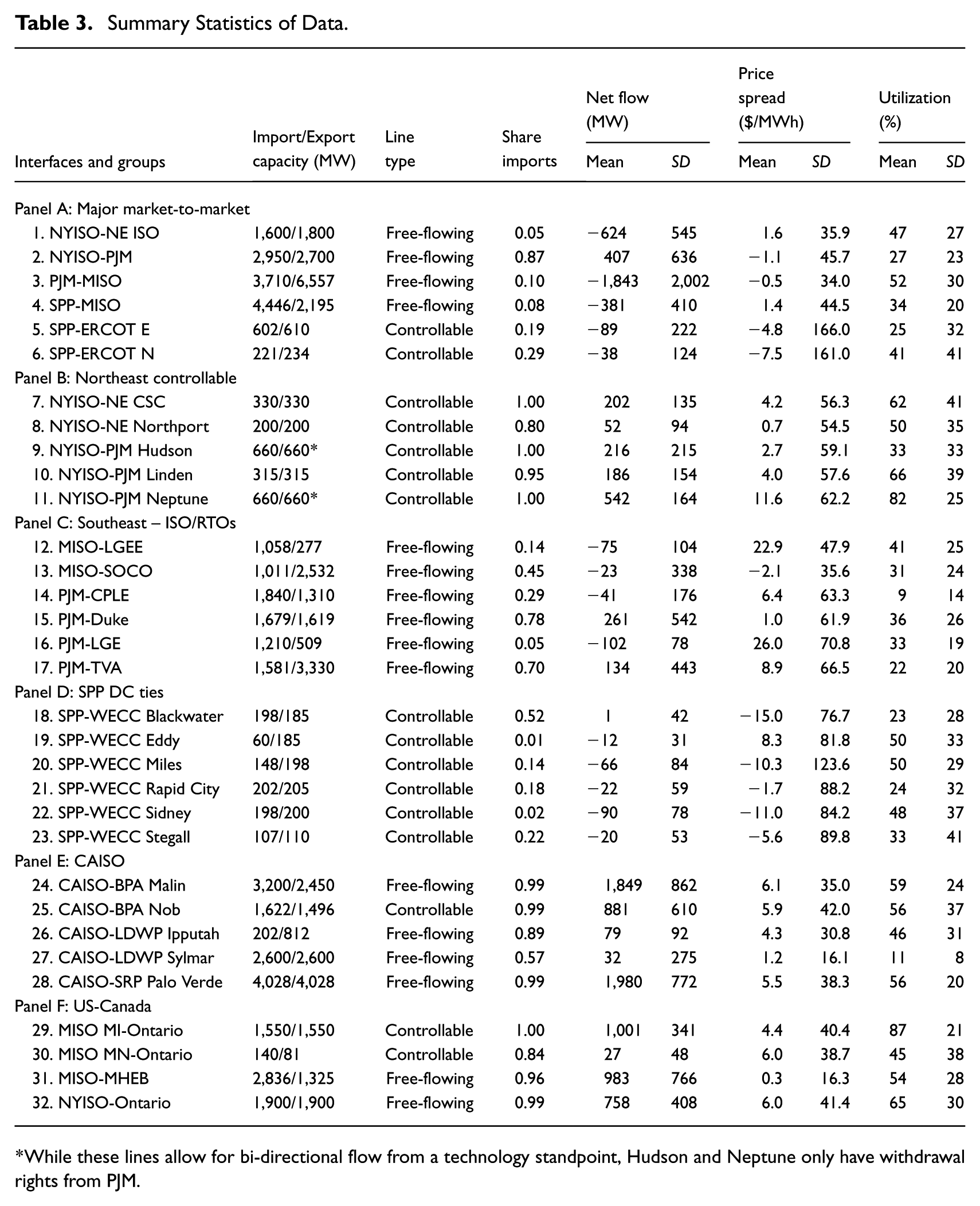
While these lines allow for bi-directional flow from a technology standpoint, Hudson and Neptune only have withdrawal rights from PJM.

2.2. Power Flow

We utilize hourly data on real-time net flow on each interface. Positive flow indicates net import to the first listed region in each of the interface name, such that, for example, a positive value of net flow on the “NYISO-PJM” interface indicates that, on net, electricity flowed from PJM into NYISO. When available, we report scheduled real-time flows. This choice minimizes the impact of loop flows – unscheduled flows along an interface that result from scheduled flow in a nearby area – on our analysis. However, if scheduled real-time flows are not available, we report actual real-time flows. Table 1 lists the transmission path and type of flow used in our analysis for each interface. In the Supplemental Information, Figure 18 presents a sensitivity analysis on the choice between scheduled and actual flows for a key result for the interfaces where both are available. In most cases the results are not sensitive to this choice; however, the choice has a significant impact on the MISO MN-Ontario interface and some interfaces between PJM and neighboring utilities in the Southeast. The latter is consistent with the finding in (Monitoring Analytics, LLC 2023) that PJM’s SOUTH interface pricing point had the largest loop flows of any interface pricing point, resulting in net actual interchange more than twice the net scheduled interchange in 2022.

2.3. Prices

We assign two prices to each interface with the goal that the difference between these two prices captures the scheduling incentive on the interface. Regional differences in market structure and terminology necessitates tailored approaches to assigning interface price pairs:

Major market-to-market, Northeast controllable: When the interface connects two US-based ISOs, our proxy for the electricity price in each region is the nodal pricing point that each ISO assigns to the interface. Consider, for example, the NYISO-PJM interface which connects two ISOs: New York ISO and PJM. NYISO has a nodal price called “PJM” that is used for imports or exports along their interface with PJM, and so we use NYISO’s “PJM” interface pricing node to represent the price of electricity in NYISO at this interface. We identify the pricing points assigned to each interface by consulting market monitor reports and other technical documents released by the ISOs.

US-Canada: Interfaces between the US and Ontario (IESO) use the same methodology as the major market-to-market and Northeast controllable groups. Because Manitoba does not have a separate wholesale electricity market, the MISO-MHEB interface pairs MISO’s MHEB interface price with MISO’s Minnesota Hub price to capture the incentive within MISO of exporting to MHEB.

Southeast ISO/RTO interfaces: These interfaces connect the wholesale market footprints of PJM and MISO to utilities in the Southeastern U.S. that are not wholesale market participants. The price node for the market side of the interface is always the interface price assigned by the ISO or RTO to the corresponding southeast utility: For PJM, this is the SOUTH interface in all cases we study. For MISO, there are distinct SOCO and LGEE interface prices. The value used for the non-market side of the interface is the utility’s hourly incremental cost of energy known as the “system lambda” as reported in FERC Form 714.

Southwest Power Pool DC ties to West: SPP has a distinct interface price node for each DC tie that we use to represent the SPP side of the interface (e.g., BLKW for Blackwater, RCEAST for Rapid City). When the utility across the tie from SPP participates in the Western Energy Imbalance Service market (WEIS) administered by SPP, we pair a relevant WEIS price with the SPP interface price. This is the case for the Rapid City, Stegall, and Sidney ties. For the other three ties, we use FERC system lambda data, as in the Southeast.

California ISO: The relevant price (i.e., “scheduling point name”) in the adjacent balancing area associated with a specific interface (i.e., “intertie constraint”) is reported by CAISO in (California ISO 2024b). These prices are each paired with a zonal price node within CAISO that was selected based on the set of connected substations shown in (California ISO 2024a).

As outlined above, we primarily utilize electricity prices from wholesale markets. Specifically, we focus on hourly average real-time prices, with day-ahead prices considered as a sensitivity case. Nodal prices – also known as locational marginal prices – reflect the marginal cost of delivering electricity to a given location in a wholesale electricity market where generation resources are dispatched by the system operator in the order of least cost. Because transmission constraints within a region can make it infeasible for least cost generation to reach local demand, nodal prices can vary within a region. In the context of interregional transmission, a price assigned by an ISO to an interface will reflect the price of trade with the neighboring system. Outside of a wholesale market, system lambdas are the closest analog to the average system price, as they represent the marginal cost being used for the economic dispatch of thermal generators (FERC 2021). However, they differ from interface prices because they are a marginal cost, not a marginal price, and they reflect the aggregate system, not an interface specifically.

There are a number of challenges associated with the accurate construction of interface pricing nodes. In order to model changes in transmission constraints due to net interchange, each ISO must make assumptions about which generation ramps down (up) in response to imports (exports) from the external region (Potomac Economics 2020). For example, PJM’s MISO interface price is the straight average of ten bus-level price nodes and PJM’s NYISO interface price is a weighted average of four bus-level price nodes. In this paper, we do not assess the efficacy of interface price definitions themselves, rather we base our analysis on the prices currently in use.

Finally, we converted IESO prices from CAD to USD based on daily exchange rates published by the Bank of Canada and then standardized all prices to real $2023-terms using a U.S. GDP-based deflator conversion. Table 1 lists the price nodes used for each interface.

2.3.1. Limitations of Energy Price Signals

While resource adequacy, resilience, and risk mitigation are priced into wholesale energy markets to varying degrees, energy prices alone are not sufficient to ensure all system needs are met. Thus, there are additional market products such as operating reserves and markets or bilateral contracts for long-term capacity commitments and power purchase agreements. These signals, which are not considered in this analysis, may help explain the interchange transaction decisions of specific actors. However, from the system perspective on an operational timescale, energy prices are the most direct measure of the impact of changing supply and demand at different places in the grid. The gains and costs discussed in this work only reflect values beyond generation costs to the extent that they are reflected in energy prices. Additionally, sub-hourly price dynamics that differ from what is captured by hourly average prices are out-of-scope.

2.4. Interface Capacity

Interfaces capacities, which may vary over time due to infrastructure changes (e.g., construction or decommissioning of transmission lines) and seasonality, are established in order to assess interface utilization. For three system operators, we obtained data on interface flow capacity through their reported hourly total transfer capability: New York ISO, California ISO, and Ontario ISO. Total transfer capability (TTC) is the maximum amount of power that can be transported on the lines connecting the two balancing authorities under reasonable system conditions. This measure of capacity is different from operational transfer capacity which adjusts the line capacity in response to seasonal line deratings and outages.

For interfaces that are not connected to the three ISOs listed above, we impute seasonal interface import and export capacities using the 99th percentile of observed flow in each direction within the season. Using the 99th percentile instead of the maximum value safeguards against outliers that may be data errors; a similar approach was used in (Deyoe et al. 2024). A season is defined as a six-month period, with the Spring/Summer season ranging from April-September of a given year and Fall/Winter ranging from October-March of the following year. We selected two seasons because ISOs conduct thermal transfer capability studies separately for Fall/Winter and Spring/Summer months. The resulting capacities can be lower than what is generally reported, for example, SPP states that it has over 6,000 MW of AC interties with MISO (Southwest Power Pool 2023), yet the largest import or export capacity we calculate for the SPP-MISO interface is 4,446 MW. This difference could be because we are using net flows or because the infrastructure was not close to fully utilized for at least 1 percent of any season. In 2023, the U.S. Congress enacted legislation directing NERC to conduct a study of the current total transfer capability between each pair of neighboring transmission planning regions (NERC 2024). The results based on simulations designed to reflect summer 2024 and winter 2024/2025 are not directly applicable here, because there is not a one-to-one correspondence between the interfaces studied here and the FERC Order 1000 planning areas used in NERC’s study and because of the different time frame.

We interpret periods where an interface has zero import and export capacity (i.e., TTC of zero or zero flow in > 99% of hours that season) as transmission outages and omit them from our sample (2.4% of hours). We also omit the 0.08% of hours where the implied interface utilization is greater than 1.3, as it is improbable that net flow would exceed the interface capacity by such a margin.

3. Analysis Framework

Conclusions in this paper are drawn from the magnitude and direction of price spreads, the magnitude and direction of net energy transfers, and how these variables coincide. Consider the examples in Supplemental Figure 12 that illustrate the relationships between price spreads and energy transfers for two interfaces between NYISO and ISO-NE. On the major ISO-NE – NYISO interface (Figure 2a), energy predominantly flows from NYISO to ISO-NE, but NYISO imports of <500 MW are not uncommon. Flow on the Cross-Sound Cable (Figure 2b) is unidirectional; the nonnegative vertical axis shows that NYISO always imports energy from ISO-NE, with power flow almost always either at capacity (330 MW) or 0. In contrast, for both interfaces, the distribution of price spreads is centered near $ 0 and each side is higher-priced in a similar number of hours, though very large price spreads (≥$50) are usually due to a higher interface price in NYISO. The imbalance of power flows with respect to price spreads in Figure 12 reveals some surprising patterns. Hours in the lower right quadrant of Figure 2a correspond to ISO-NE importing energy from NYISO, even though it is more expensive. Similarly, at the top of the heatmap in Figure 2b, we see that there are hours in which NYISO is maximally importing on the Cross-Sound Cable, despite being on the lower side of the price spread.

Figure 2.

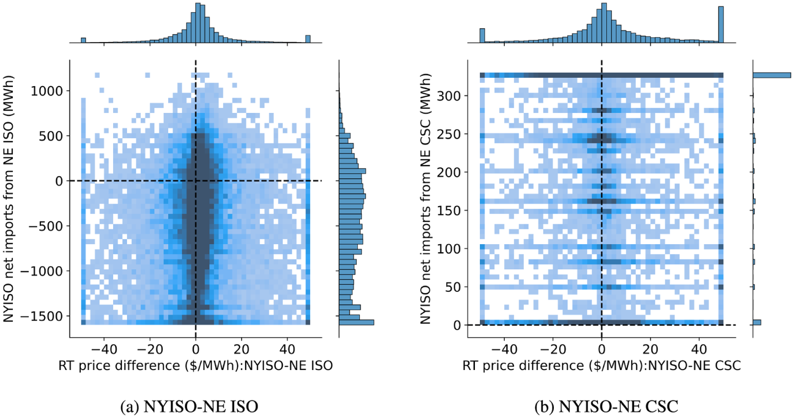
Distribution of hours during 2021 to 2023 according to observed price spread and energy transfer on two interfaces. (a) NYISO-NE ISO and (b) NYISO-NE CSC.

Figure 3 compares the directional balance of power flow and price spreads for all interfaces in this study. The left column, a value of 1 reflects an interface where power always flowed in the same direction, for example NYISO-ISONE CSC; a value of 0.5 reflects an interface where power flowed in each direction 50 percent of the time. This study includes interfaces across this spectrum. We can also infer an expected direction of power flow in each hour based on the low-to-high price direction and, in turn, an expected level of balance which is shown in the right column of Figure 3. A line crossing 0.5 corresponds to an interface where the side that typically exports is expected (based on price spreads) to import the majority of the time. Again, we see some surprising patterns highlighted by steeply sloped lines. In general, these results suggest that we would expect imports and exports to be much more balanced across the seams we analyzed than what we observe empirically. Section 4 will formalize these ideas, explore interchange patterns in more detail, and quantify their impact. Section 5 will discuss the economic, physical, and geographic characteristics that may contribute to the observed patterns.

Figure 3.

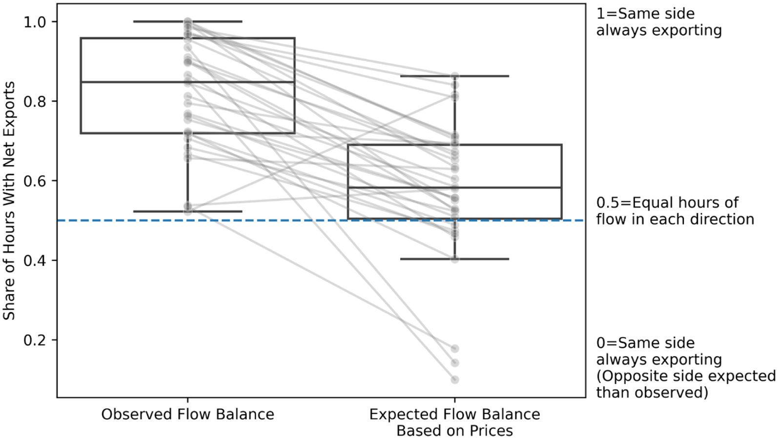
Interface balance based on the number of hours that power flowed (left) and was expected to flow (right) in each direction.

4. Measuring Efficiency in Usage of Interregional Transmission

Interregional transmission can increase allocative efficiency through static gains from trade; when price differences exist between the two regions, market integration allows for low-cost power plants to export electricity across the interface and replace higher-cost generation in the neighboring region. To study if transmission usage is efficiently coordinated between regions, we devise a simple measure of allocative efficiency by observing if the direction of net scheduled flow on the interface is consistent with the direction of real-time prices in that hour. We use this measure to categorize flow in each hour as being “economic”– when electricity is imported by a region with comparatively higher prices – or “uneconomic”– when electricity is imported by region with comparatively lower prices. Table 4 lists how we categorize flow under all possible combinations of price differences and net flow directions.

Table 4.

Definition of Economic Flow Between Regions A and B.

Direction of prices in regions A and B	Net flow direction with respect to region A	Flow type
A > B	Import	Economic
A < B	Export	Economic
A = B	Any	Economic
A < B	Import or 0 net flow	Uneconomic
A > B	Export or 0 net flow	Uneconomic

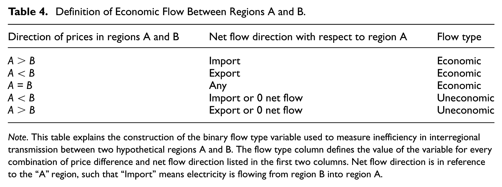
Note. This table explains the construction of the binary flow type variable used to measure inefficiency in interregional transmission between two hypothetical regions A and B. The flow type column defines the value of the variable for every combination of price difference and net flow direction listed in the first two columns. Net flow direction is in reference to the “A” region, such that “Import” means electricity is flowing from region B into region A.

This categorization is defined from the centralized perspective of a combined two-region system operator seeking to minimize total energy generation costs. While bilateral contracts and other out-of-market hedging mechanisms are important to how individual actors make decisions and categorize system outcomes, they are not relevant to the centralized operator perspective taken here. The need for and costs of other services including frequency regulation, operating reserves, ramping, black start, and capacity obligations are not directly considered. Instead, they are only accounted for to the extent that they affect energy prices, as discussed in section 2.3.1. The focus on energy is justified because it is the predominant component of the all-in price of electricity. (For ERCOT, MISO, PJM, NYISO, ISO-NE, and SPP in 2020–2022, energy typically made up 85 percent of the all-in price, with capacity being the next-largest cost contributor [Potomac Economics 2023a]). An analysis of the efficiency of interregional transmission when used for additional electricity system services is left for future work. The role of time-coupled constraints, such as generator ramping or minimum run time requirements, on the economics of commitment and dispatch decisions is also left for future work; this analysis considers each hour independently.

We divide our analysis into two sections: (a) periods with economic flow and (b) periods with uneconomic flow. In the first section, we quantify the benefits realized by economic flows, measure each interface’s utilization rate during these periods, and quantify the opportunity cost of underutilization. In the second section, we examine the prevalence and cost of uneconomic flow and test these findings for sensitivity to the choice of market time frame (i.e., day-ahead vs. real-time). Finally, we summarize the quantitative results for the historical status quo and the opportunities to increase value from the existing interface infrastructure.

4.1. Economic Interchange

During periods of economic flow, trade can lower the overall cost of electricity by enabling lower-cost power plants to produce a greater share of the power needed than would otherwise be used within one region. Still, even economic flows (as defined in Table 4) may not be perfectly efficient. Specifically, if an interface’s flow is below its transfer capacity and a significant price difference persists, then the interface is likely underutilized. In this section we examine the benefits that these interfaces delivered and their utilization rates.

We estimate the gains from trade on interface i connecting balancing authorities l and j in year t as the sum over the hours of the year, $H$ _t , of the price spread between the two regions multiplied by volume of economic imported electricity:

\begin{matrix} Gains from economic flo w_{it} = \sum_{h \in H_{t}} 1 (flow typ e_{ih} \\ = Economic) \cdot | net flo w_{ih} | \cdot | pric e_{ilh} - pric e_{ijh} | \end{matrix}

(1)

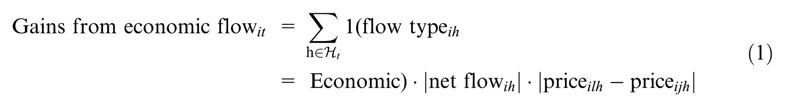
This calculation assumes that the observed price difference would be unchanged if all power flow on the interface was eliminated. The price difference would likely increase if the flow was reduced due to changes in each region’s marginal generator, so this is a conservative estimate of the gains. A sensitivity analysis conducted in the Supplemental Information uses an assumed linear rate of price convergence based on (Kemp et al. 2025) and estimates gains from economic flow that are 15% greater than those calculated using (1) for the median interface.

Over the 2014 to 2023 period, gains from economic flow summed across all thirty-two interfaces was $1.23 billion per year on average. Figure 4 plots the average annual gains per unit of transfer capacity at each interface, obtained by scaling equation (1) by the interface’s annual transfer capacity to allow comparison across differently sized interfaces. Higher bars indicate interfaces where, on average, net flow led to greater gains relative to available transfer capacity. The interfaces that produce the greatest per-capacity gains from economic flow are all controllable interfaces – those between SPP and ERCOT, between NYISO and PJM or ISO-NE, three of the DC ties between the eastern and western interconnect, and the DC line between CAISO and the Nevada-Oregon Border (NOB). Additionally, there are reliability, resilience, and resource adequacy benefits provided by these interfaces that are not fully captured by energy market prices. The annual values across the study horizon are provided in the Supplemental information.

Figure 4.

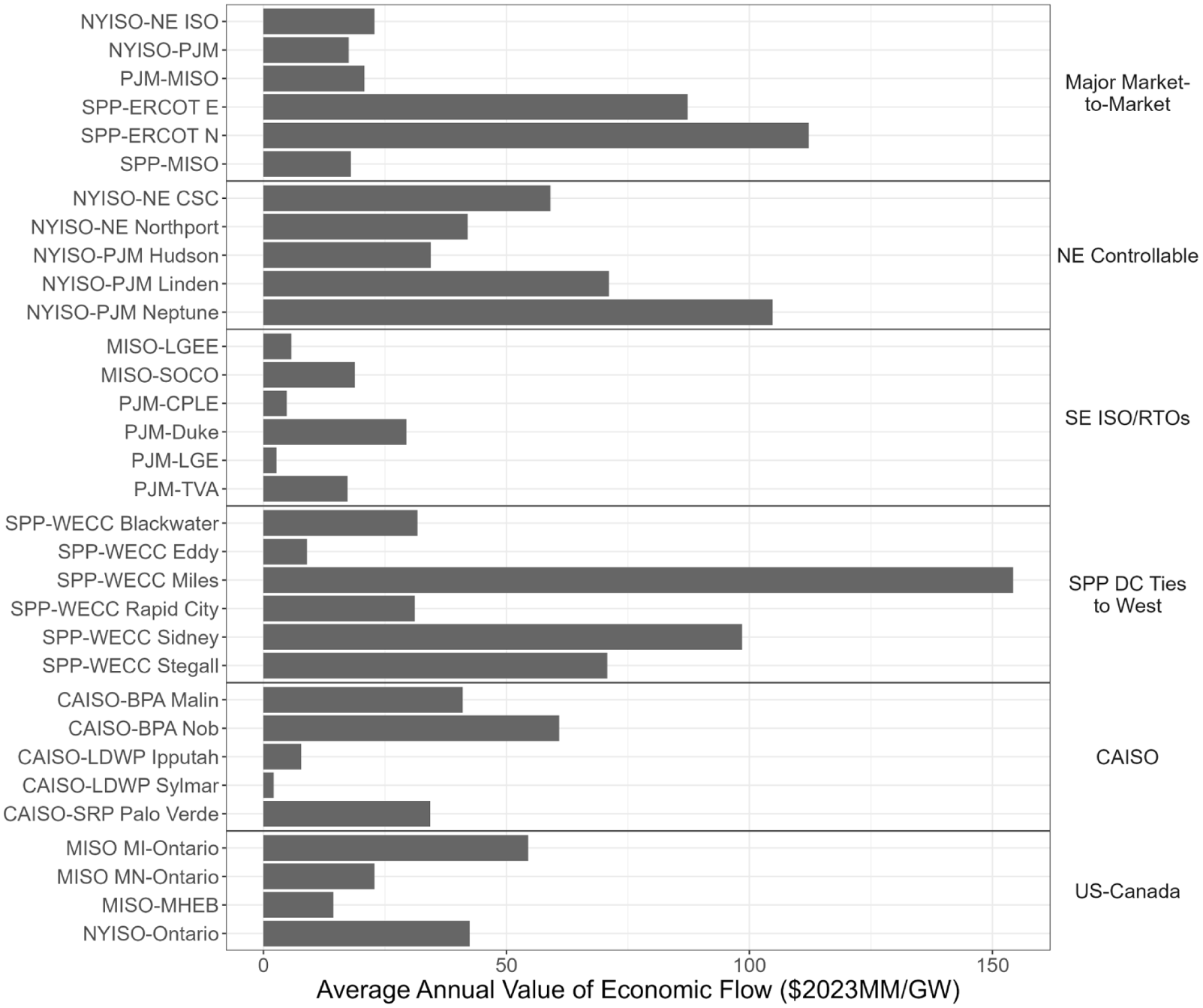
Value of gains from economic flow per gigawatt of transfer capacity.

4.1.1. Interface Utilization

When lines have spare capacity, gains from trade can theoretically increase if that capacity is used to transfer additional power from low to high price regions. In an idealized economic model, we would expect transmission constraints to bind (i.e., flow to hit the capacity or ramping limit) unless prices between the markets have converged (i.e., the price spread is $ 0). Therefore, even when energy flows in the economic direction, it still may be inefficient if price convergence has not been achieved and there is available, unused capacity on transmission ties. A positive correlation between interface utilization and price difference magnitude would indicate a level of price responsiveness, even if utilization is lower at small price differences due to other factors.

Figure 5 shows interface utilization segmented by price difference magnitude when flow is economic. Here, utilization is defined as the ratio of the magnitude of net flow to the current interface capacity in the direction of net flow. Utilization values over 100% are not unexpected due to the interface capacity methodology detailed in Section 2.4. Some interfaces are highly utilized, regardless of the price difference, for example, CAISO-BPA NOB and some of NYISO’s controllable interfaces with PJM and ISO-NE. Other interfaces typically have low or moderate utilization regardless of the price difference, such as CAISO-LDWP Sylmar, PJM-CPLE, and SPP-WECC Rapid City. Finally, utilization on some interfaces is positively correlated with the price difference: the SPP-ERCOT N interface is the quintessential example, while SPP-ERCOT E, NYISO-PJM, NYISO-NE ISO, NYISO-NE Northport, and SPP-WECC Stegall are all examples of more muted versions of this pattern. The interface-level utilization rates for each year of the study horizon during hours with a price spread of at least $20/MWh are provided in Supplemental information Figure 15.

Figure 5.

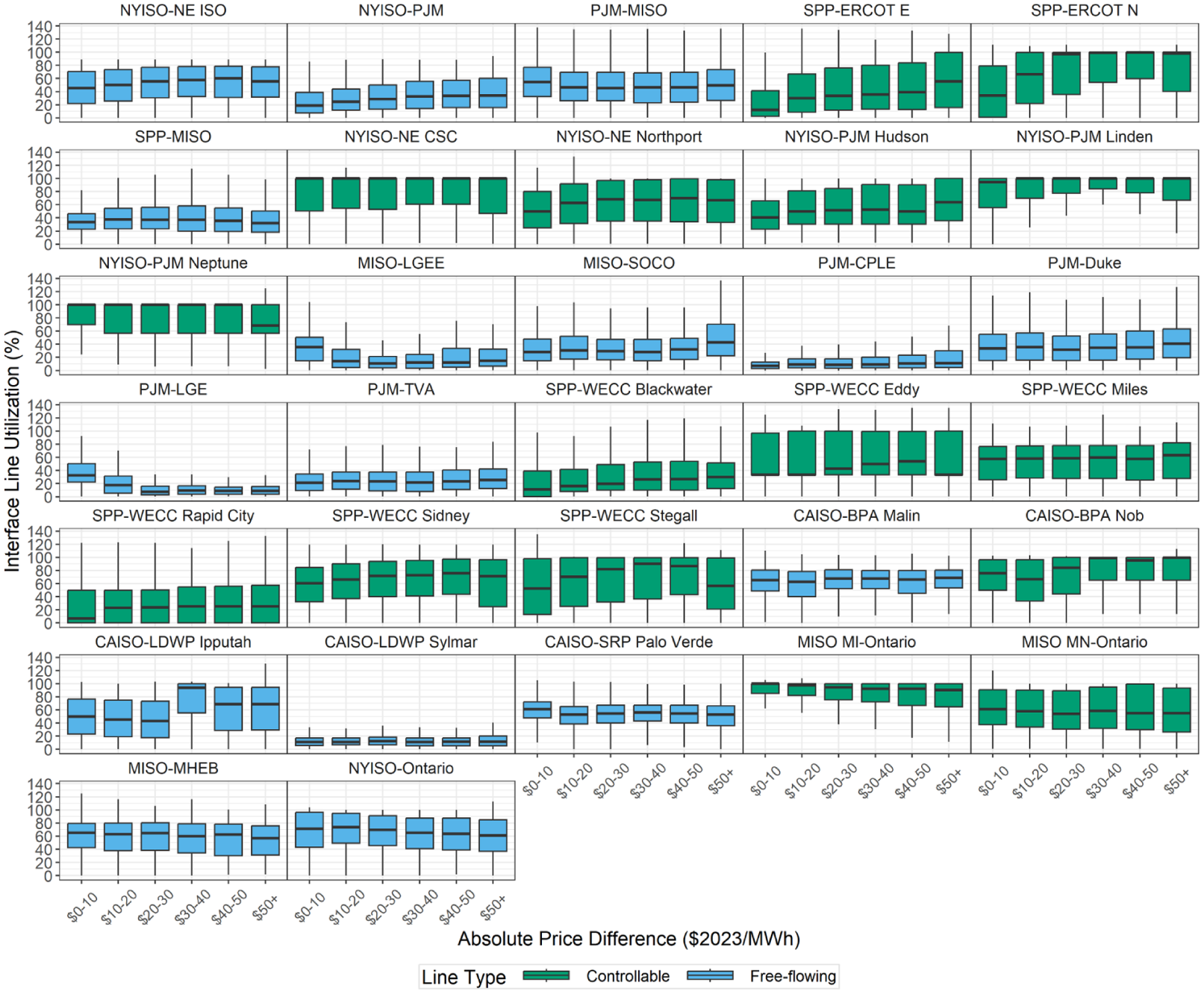
Interface utilization segmented by price spread when flow was economic.

Increasing interface utilization is one way to increase the value an interface provides. A utilization increase of 20 percentage points up to a maximum of 100% during hours with a price spread of at least $20/MWh would have raised the value during economic hours by 19% on average, an aggregate opportunity across the thirty-two interfaces of $238 million per year on average. Figure 6 shows the relative size of this opportunity for each interface. In the terminology of equation (1), this consists of increasing |net flow| _ih when the first term of the summation is 1. As increasing economic flow could reduce price spreads, an effect not modeled here, this marginal opportunity value is an upper bound. A sensitivity analysis conducted in the Supplemental Information uses an assumed linear rate of price convergence based on (Kemp et al. 2025) and estimates an opportunity value 3% less than those shown in Figure 6 for the median interface. Large step changes in generation costs – a scenario not modeled in our linear sensitivity analysis – may result in a lower value if prices converge after only a small increase in utilization. Further, it may not always be possible to increase power flow across an interface even when we observe a utilization value less than 100%, because, for example, internal constraints within one or both balancing areas can limit power flow on interfaces (Glazer et al. 2023), an interface ramping constraint may be binding, transmission capacity may be reserved to provide reliability in case of a contingency, or transmission outages may exist. This analysis hedges against these factors by providing a high-level estimate of the opportunity associated with a moderate improvement in interface utilization during a minority of hours.

Figure 6.

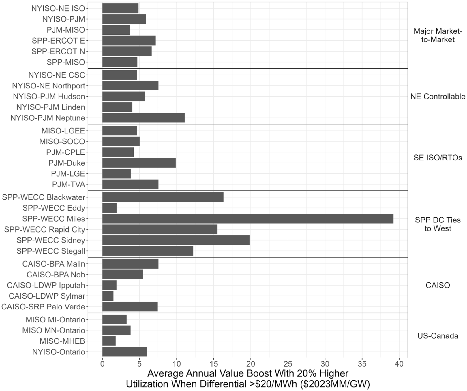
Impact of increasing interface utilization by 20 percentage points (e.g., moving from 50% to 70% utilization) when the price spread is over $20/MWh.

4.2. Inefficiency Due to Uneconomic Interchange

Despite the significant gains from interregional trade, we find that 26% of all interregional electricity flows by volume in our sample are uneconomic, which we interpret as evidence that there is substantial inefficiency in the usage of the interregional transmission capacity. However, as Figure 7 shows, this number masks the heterogeneity at the interface level, where the share of uneconomic flow ranges from 11% to 81%. This share of energy transferred on an interface that is uneconomic (Figure 7 blue bars) is often lower than the share of time with uneconomic flow (Figure 7 black crosses), indicating that uneconomic flow is more common in hours with lower flow volumes.

Figure 7.

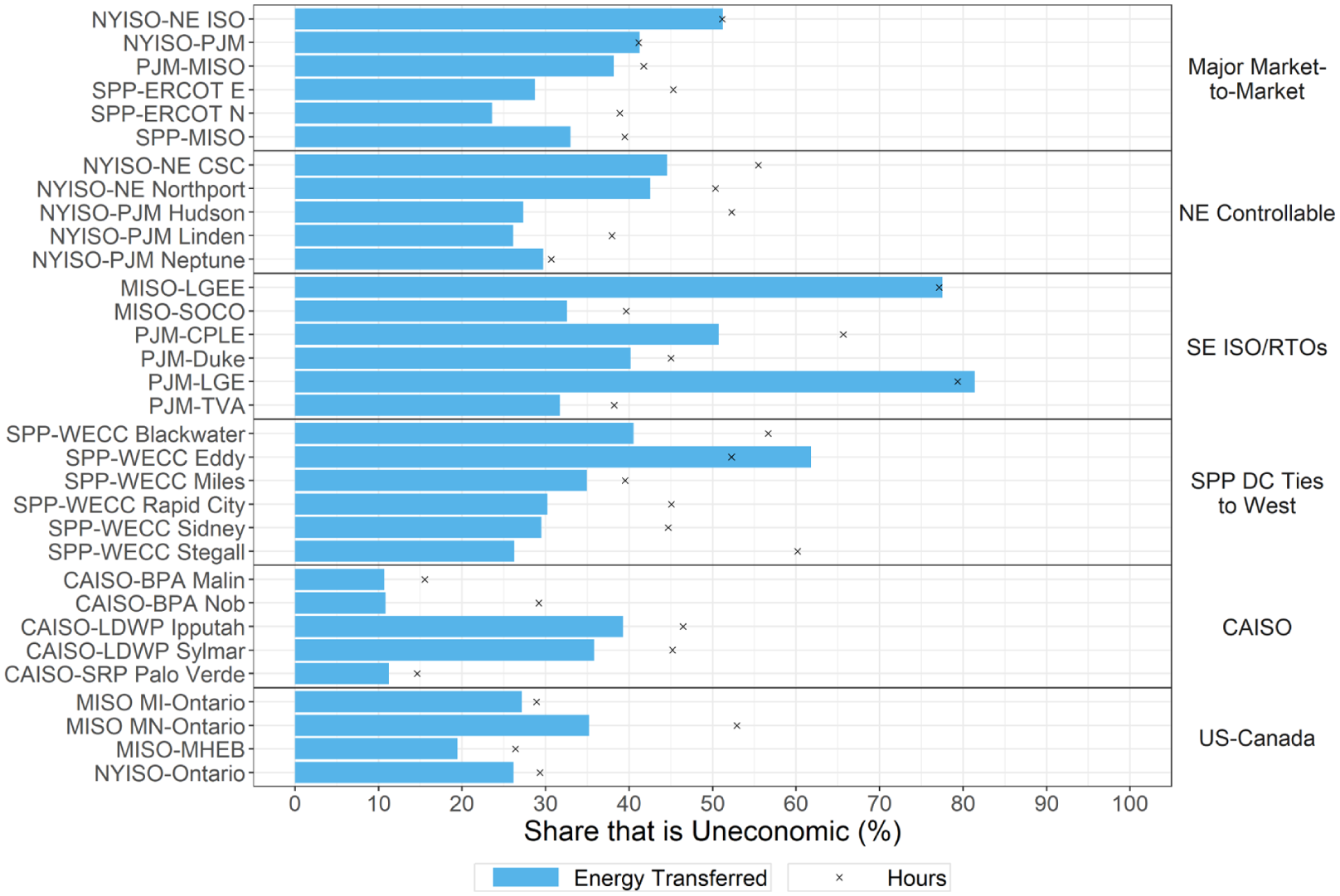
Prevalence of uneconomic interchange.

4.2.1. Relationship Between Price Spreads and Interchange Economics

Our preferred measure of efficiency implicitly weights hours with larger flow volumes more highly than those with lower volumes – we care more about the total share of energy that is uneconomic, not the total share of hours, some of which may have very little net flow at all. However, another critical factor in determining the level of efficiency is the magnitude of the price difference during a given hour. Uneconomic flow during hours where price differences between the two regions are large can lead to greater inefficiency as within-region generation is offset by out-of-region electricity that is significantly more expensive. For example, the contribution of uneconomic flow to inefficiency will be higher when out-of-region generation is priced $30 higher than when it is only priced $1 higher. If uneconomic flow is concentrated during low price difference hours, the economic cost may not be high. Studying the usage on transmission lines during extreme pricing periods is particularly relevant because previous work suggests that 45 percent of transmission’s congestion value comes from only 5 percent of hours (Kemp et al. 2025).

We test whether uneconomic flow persists during high-value hours by comparing the distribution of uneconomic interface flow across price spread ranges. Figure 8 shows that, for most groups, the average share of energy that is transferred in an uneconomic direction exceeds 25% even when the price difference between regions exceeds $50/MWh. A price spread of $50+ is large compared to the average observed absolute price difference of $16/MWh. While the share of uneconomic flow decreases or remains flat as price differences grow for most groups, it is striking that the degree of inefficiency for most Major Market-to-Market interfaces rises, because flow on this group constitutes roughly one quarter of all observed volumes. If the observed flows were settled at real-time prices, this figure would indicate that for over 40% of flows scheduled during a price spread of $50+, traders were losing at least $50 on every unit. To see the trends for individual interfaces within each group and over time, we refer the reader to the Supplemental information file.

Figure 8.

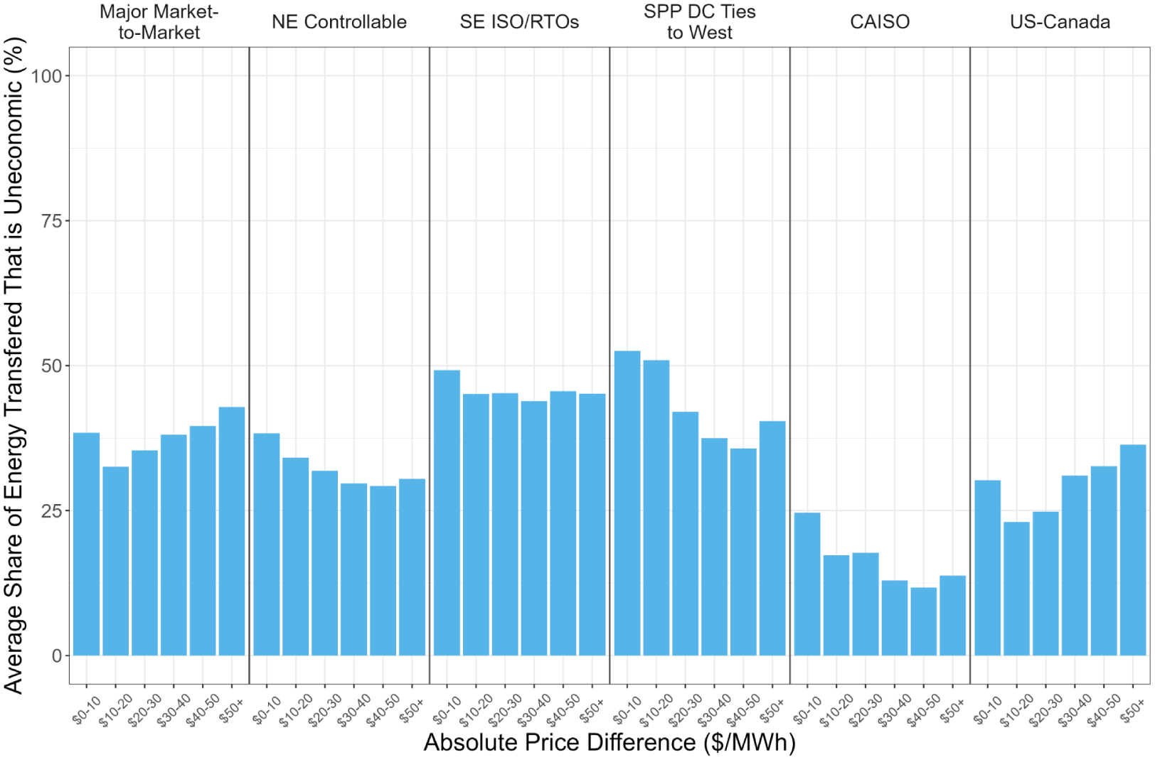
Prevalence of uneconomic flow by real-time market price spread.

4.2.2. Sensitivity to Transaction Costs

One limitation of our uneconomic flow definition is that it ignores transaction costs which may make it unprofitable to use interregional transmission when price spreads are not high enough to cover the cost of trade. In our setting, these transaction costs can include tariffs charged by ISOs on external transactions, uplifts paid as guarantees, or other kinds of charges such as CAISO’s border adjustment on its emissions trading system. Previous work has modeled interregional transmission usage under assumed transaction charges that range from $3 to $10/MWh (Pfeifenberger, DeLosa, et al. 2023; Southwest Power Pool 2020). If costs to trade are responsible for explaining our observed metric of inefficiency, we should see a large drop in the median share of uneconomic flow above $10/MWh, when price spreads are assumed to be large enough to outweigh transactional charges. Figure 8 does not find evidence to support this hypothesis, except in the case of interfaces in the CAISO group, where the average uneconomic flow share drops by over one-third as we compare hours with a price spread less than $10/MWh to those with a spread of $10 to 20/MWh or more. However, in other regions, we do not see sharp declines in our measure of inefficiency after price spreads exceed $10/MWh, suggesting that transaction costs cannot fully explain the prevalence of uneconomic flow.

4.2.3. Sensitivity to Market Timelines

Another consideration is that our measure of inefficiency determines whether flow is uneconomic from the perspective of prices settled in the real-time electricity market, despite the fact that 95% of power transactions in ISOs are scheduled in a forward electricity market known as the day-ahead market (FERC 2020). We focus on real-time prices to measure inefficiency to align with our use of real-time flows and because real-time markets are physically binding and used to balance actual demand and supply on the system, and therefore real-time prices reflect the value of delivering the marginal unit of electricity to a region. However, if the gap between real-time and day-ahead prices is sufficiently large, our measure of inefficiency may overlook the fact that interchange was economic when it was scheduled in the previous day, even if the real-time scheduled or actual flow is no longer economic according to real-time prices.

To determine if the scope of inefficiency is similar across market time frames, in Figure 9 we compare the level of inefficiency found in our main estimates using real-time prices to levels of inefficiency using day-ahead prices, where possible. The flow data used in these two cases is the same, as described in Section 2.2. Consistent with the fact that interregional flows are often scheduled in the day-ahead time frame, day-ahead prices seem to better rationalize observed net flow for some groups of interfaces, though often only marginally. The total share of uneconomic flow in our sample drops from 26% to 18% when changing the definition from real-time to day-ahead prices. Results for the Northeast Controllable group are most sensitive to the choice of reference market, with the share of uneconomic flow based on day-ahead markets typically less than half that when considering real-time. This finding suggests that some interfaces are scheduled more economically day-ahead, but lack or under-utilize the flexibility to adjust in real-time operations.

Figure 9.

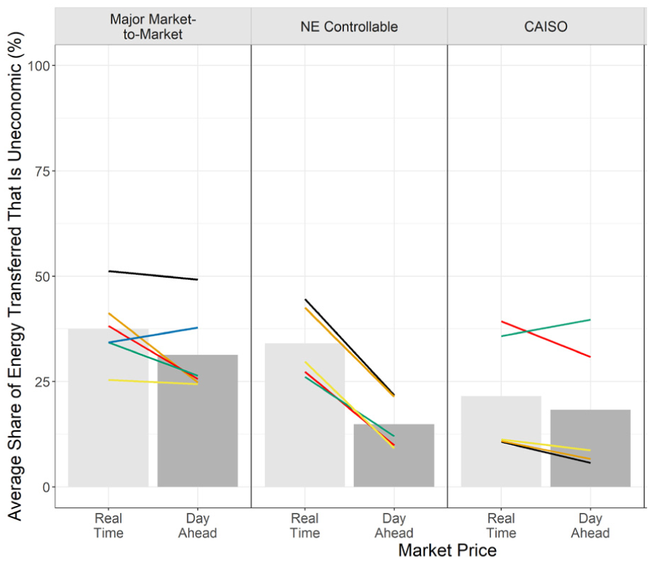
Prevalence of uneconomic flow under different definitions of market price.

4.2.4. Value from Eliminating Uneconomic Flow

We can derive an economic cost of inefficient interregional transmission usage by calculating the value of eliminating imports during uneconomic hours. Implicitly this calculation asks: what would the total savings be if regions did not import relatively expensive electricity, but instead increased generation at cheaper within-region prices? Similar to our approach for estimating the gains from economic flow, let the value of eliminating uneconomic flow on interface i connecting balancing authorities l and j in year t be the sum over the hours of the year, $H$ _t , of the price spread between the two regions multiplied by total volumes of uneconomic imported electricity:

\begin{matrix} Value of eliminating uneconomic flo w_{it} = \sum_{h \in H_{t}} 1 (flow typ e_{ih} = uneconomic) \cdot \\ | net flo w_{ih} | \cdot | pric e_{ilh} - pric e_{ijh} | \end{matrix}

(2)

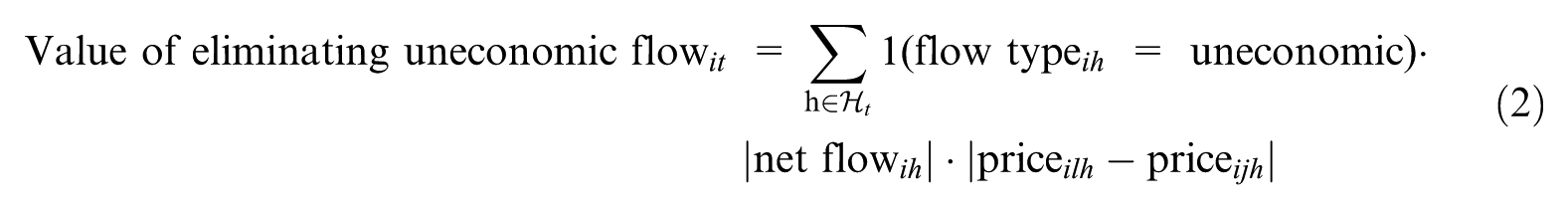
This calculation is marginal in that it assumes that the prices we observe represent the marginal cost of delivering electricity to the region around the interface and that shifting generation from out-of-region producers to within-region producers does not shift local prices. As the price difference would be expected to decrease if the uneconomic flow was reduced, this value is an upper-bound estimate. However, it is a reasonable approximation if the uneconomic net flow is a low share of within-region capacity, and (Reed and Xu 2022) found that electricity transmission transfer capacity between adjacent FERC Order 1000 planning regions was at most 20% and typically <10% of the peak load of the larger region. A sensitivity analysis conducted in the Supplemental Information uses an assumed linear rate of price convergence based on (Kemp et al. 2025) and estimates gains from economic flow that are 8% less than those calculated using (2) for the median interface. Note that this value of eliminating uneconomic flow is not the same as the value of moving from the observed flow to the optimal flow, which at times would be in the opposite direction. Instead, it is just moving from the observed flow to zero net transfer across the interface.

Using this methodology, we estimate that inefficiencies from uneconomic flow from 2014 to 2023 have led to a combined $551 million in excess electricity costs per year on average across the thirty-two interfaces. To understand which interfaces have the highest cost of inefficiency, we calculate the annual value of eliminating uneconomic flow for each interface and plot the average in Figure 10a. To compare across interfaces of different sizes, each annual value is scaled by the maximum interface capacity (see Section 2.4) in that year. Across all interfaces, the average annual value of eliminating uneconomic flow is $17 million per GW of transfer capability. The value of eliminating uneconomic flow varies significantly across interfaces and is not always highest in the interfaces with the greatest share of uneconomic flow. In particular, interfaces in the Northeast controllable group and the Miles, Sidney, and Stegall DC Ties stand out as having particularly high cost per unit of capacity, despite the share of flow that is uneconomic being similar to many other groups. This is because these interfaces are more highly utilized than others and tend to experience large price spreads during uneconomic hours, both factors which drive up per-unit costs.

Figure 10.

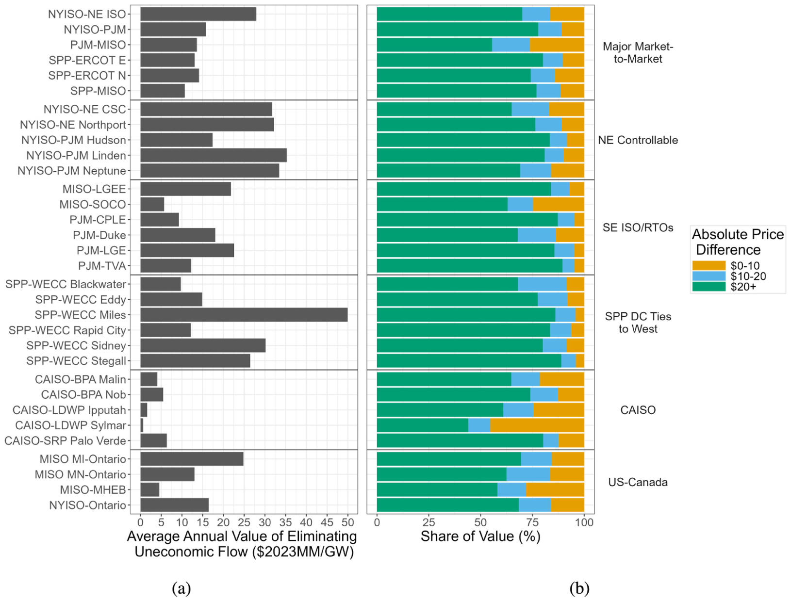
Annual value of eliminating uneconomic flow. The left panel (a) shows the average annual value of eliminating uneconomic flow on each interface per gigawatt of transfer capacity. The right panel (b) shows that the majority of savings from reducing uneconomic flow comes from hours in which the price spread is > $10/MWh, or even > $20/MWh.

Figure 10b decomposes the total cost of uneconomic flows for each tie by the magnitude of the price spread between the two regions. We plot the share of the value in the left panel that stems from hours with a price difference of $ 0 to $10/MWh, $10 to $20/MWh, and over $20/MWh to better understand the composition of uneconomic periods. For most interfaces, the majority of the cost of uneconomic flow comes from hours with a $20+/MWh price premium. Our previous finding in Figure 8 showed that uneconomic flow occurs during high-value hours. Here, we see that these hours occur frequently enough to contribute in an economically significant way to the overall cost of inefficient interface usage. The orange segments representing the cost of uneconomic flows associated with price differences under $10/MWh are relevant to the discussion of transaction costs in Section 4.2.1. If fees and tariffs on external transactions between regions are solely responsible for uneconomic flows at these price differences, then Figure 10b shows the share of uneconomic value that could possibly be recovered from changes to such policies.

4.3. Results Summary

In sections 4.1.1 and 4.2.4 we separately quantify the value of economic flow and the cost of uneconomic flow for each interface relative to its size. In aggregate, we find that these thirty-two interfaces delivered average net gains of $674 million per year, as shown in the green bar in Figure 11. For reasons discussed previously, this value is likely a conservative estimate. Due to differing study horizons for different interfaces there are multiple potential approaches to calculating an overall average annual value. Here, we sum the average value for 8,760 hours for each interface, where the average is taken over the study horizon. We also measured the impact from two sets of changes to interregional interchange that could increase the value provided by the existing infrastructure. These opportunities for increased value are additive, not mutually exclusive.

Figure 11.

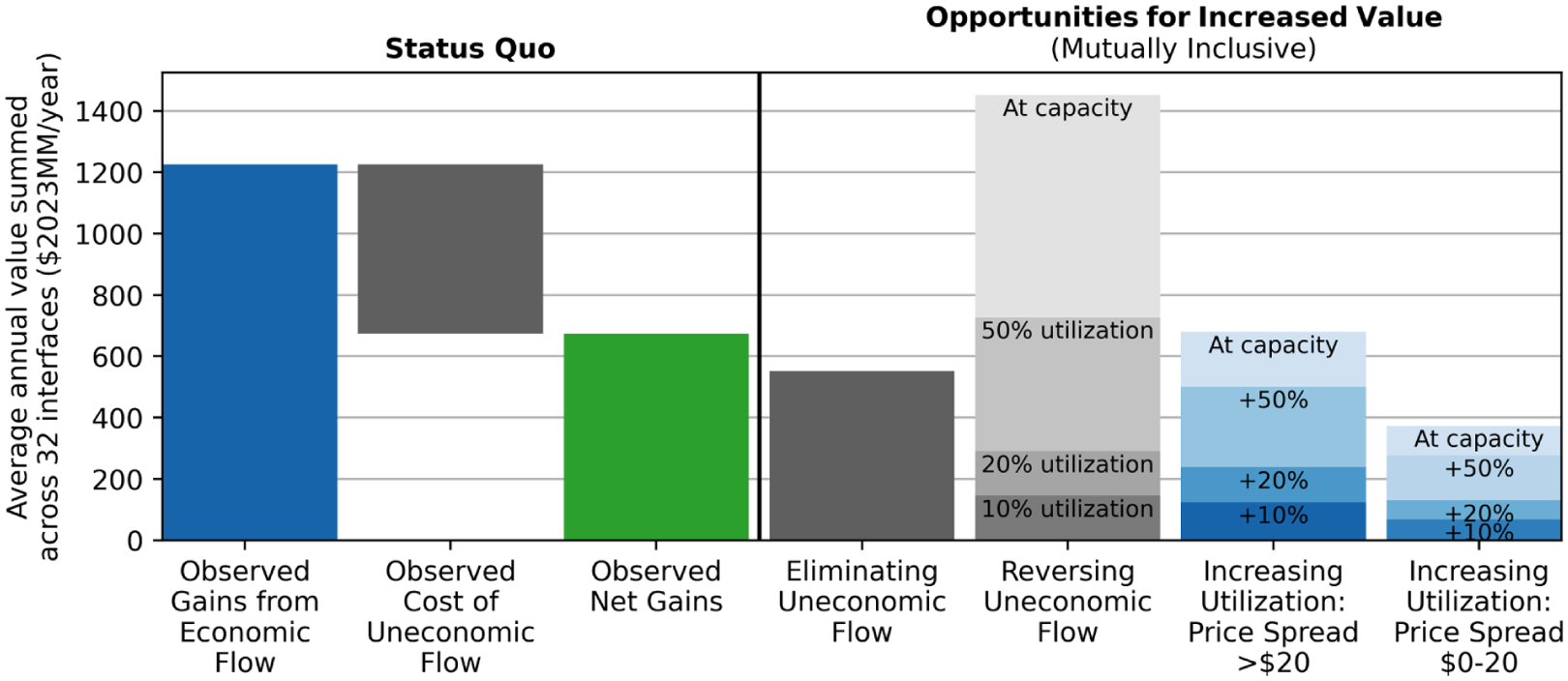
Results summary.

The first change to interregional interchange is increasing volumes when flow is in the economic direction. The value of increased economic flow depends on the level of utilization achieved and whether the utilization increases are concentrated in hours with large price spreads, as shown in the rightmost blue bars in Figure 11. For example, increasing utilization by 20 percentage points when the price spread was over $20/MWh for all thirty-two interfaces could increase gains by $238 million per year on average. The feasibility of increasing utilization depends on interface ramping, reliability, and within-region transmission constraints, as discussed in Section 4.1.1. Because prices will eventually converge given sufficient interchange, there is greater uncertainty in this value assessment (which does not account for price convergence) at higher levels of volume change and when the price spread was smaller to begin with. A first-order estimate of this opportunity size for all interfaces in the continental U.S. and in-scope U.S.-Canada interfaces (i.e., not only the thirty-two interfaces studied here) is $400 million per year, based on the 60% coverage rate of the thirty-two interfaces discussed in Section 2.

The second set of changes to interregional interchange address uneconomic flow. The value of eliminating uneconomic flow for all thirty-two interfaces as defined and discussed in section 4.2.4 is $551 million per year on average (first-order estimate of $920 million per year for all interfaces in the continental U.S. and in-scope U.S.-Canada interfaces). This value is based on a methodology that considers each hour independently, and it may include some flow that was rationalized by time-coupled constraints. In virtually all cases the optimal interchange in these periods would not be zero (the result of eliminating uneconomic flow) but some flow level in the opposite direction. We do not attempt to determine this optimal level; instead, we estimate the gains from various volumes of economic flow in Figure 11. Similar to increasing utilization for flows that were already economic, uncertainty in this value assessment increases with the magnitude of the change. Assuming prices remain at observed levels associated with uneconomic flow, economic flow at 10% utilization during the same periods would be worth $97 million/year on average (first-order estimate of $160 million per year for the all interfaces in the continental U.S. and in-scope U.S.-Canada interfaces).

The magnitude of these opportunities motivates additional research on market and technology solutions to improve the efficiency of interregional electricity trade in the U.S.

5. Discussion

We have presented evidence that suggests 26% of all net flow on the interfaces we study between 2014 and 2023 displaces relatively cheaper within-region generation with more expensive generation and that most interfaces are regularly underutilized, even when the energy being exchanged is economical. However, our results also show significant heterogeneity in the level of inefficiency by interface. Here we discuss a number of economic, physical and geographical features of interfaces that may contribute to interface efficiency and explain differences in our findings across groups of interfaces.

5.1. Controllable Interfaces

On interfaces with some controllable element, 25% of flow is uneconomic, compared to 26% on free-flowing interfaces. That interfaces with controllable power flow have similar levels of uneconomic flow as free-flowing interfaces suggests that adoption of controllable line technology is not sufficient to create the conditions under which market participants will maximize real-time gains from trade.² However, in the northeast where NYISO has both types of interfaces with PJM and ISO-NE, free-flowing interfaces do have greater levels of uneconomic flow than controllable interfaces between the same markets: at least 10 percentage points greater for PJM-NYISO interfaces and 5 percentage points for ISO-NE-NYISO interfaces.

Our results suggest that controllable line technology does affect interchange on other measurable dimensions. Specifically, controllable interfaces are utilized more fully during economic hours: an average of 62% relative to 47% for free-flowing interfaces. Put differently, if market structures foster economic interchange, participants choose to take greater advantage of interregional lines when power can be directly delivered from source to sink.

5.2. Market Design

A natural question is whether interfaces that have adopted more coordinated scheduling mechanisms have more efficient outcomes. Several of the free-flowing interfaces in the “Major Market-to-Market” group we study (i.e., NYISO-NE ISO, NYISO-PJM, and PJM-MISO) allow generators to trade power through a market dispatch mechanism known as Coordinated Transaction Scheduling (CTS) which “relies on forecasted prices to allow bilateral market participants to project whether a submitted intertie transaction would be profitable in the real-time market” (Pfeifenberger, DeLosa, et al. 2023). Previously, Pfeifenberger, DeLosa, et al. (2023) demonstrates the negative impact of latency on effective scheduling and Ndrio et al. (2022) developed a game-theoretic model of CTS to show that market efficiency degrades with liquidity shortfall and transaction costs. We find that even in these markets, 38% to 51% of flow volumes ultimately increase system costs.

The efficiency of interfaces using CTS depends on how the CTS mechanism is designed and used. While MISO and PJM began using CTS in 2017, the MISO market monitor reports that participation remains extremely minimal even in 2022 and that “high transmission charges and persistent forecast errors” are likely to have contributed to the low utilization of the process (Potomac Economics 2023a). The ISO-NE market monitor highlights that “many CTS participants take on day-ahead positions and offer price-insensitive real-time bids and offers,” with over half of CTS transactions in 2022 willing to clear at greater than a $25/MWh loss (Potomac Economics 2023c). Others have also noted that excessive transmission charges, the quality of forecasted prices, and the frequency of scheduling may limit the ability for CTS to optimize power flows between regions (Pfeifenberger, DeLosa, et al. 2023; Potomac Economics 2023b; Southwest Power Pool 2020).³ While we do not evaluate CTS directly in this study, our results are in line with previous work that finds that the efficacy of CTS in coordinating gains from trade may be limited by its design and uptake by market participants.

California ISO also operates a market within the western United States that coordinates interface flows known as the Western Energy Imbalance Market (WEIM). Created in 2014, the WEIM allows for sub-hourly least-cost dispatch on the interregional transmission capacity that remains available after scheduled flows are cleared, similar to the real-time market dispatch mechanism that ISOs themselves use within a balancing region. CAISO-BPA Malin, CAISO-BPA NOB, and CAISO-SRP Palo Verde have the lowest rates (11%) of uneconomic flow of any interfaces we studied. The remaining interfaces that involve CAISO have around average rates of uneconomic flow, but they do appear to be price responsive with generally decreasing rates of uneconomic flow as price spreads increase. Note that we have not tested the extent to which these results are attributable to the WEIM or to other factors.

5.3. “Winners” and “Losers”

This paper examines efficiency from the point of view of a combined two-region system for each interface. While eliminating uneconomic flow would lower the total cost of electricity production across the combined system, it would not impact all parties equally. For example, if Region A is exporting to Region B despite having a higher marginal price, eliminating that flow would lower and raise revenues for the marginal generators in Region A and B, respectively. Further, the change could be large enough to affect electricity prices. While we leave an investigation into specific winners and losers of changes in interchange patterns for future work, it is important to note that efficiency improvements from the system perspective may present as positive or negative changes to different groups of producers and consumers.

6. Conclusion

This study analyzes data on energy transfers and nodal prices and finds inefficiencies in interregional transmission usage within the United States’ electricity system. We estimate the impact of economic and uneconomic flows across market seams and find that the cost of inefficiencies is large. Aggregating the thirty-two interfaces we study, the average cost savings achieved is at least $1,226 million per year, but that positive impact is offset by an average annual cost of uneconomic flow of $551 million. Additional value could be enabled by increasing utilization. Notably, uneconomic flows and low utilization rates can persist even during hours where the price spread between regions are large. We also explore key factors that may contribute to these inefficiencies, including differences in market operating rules and technologies.

Our findings highlight an immense opportunity in improved usage of interregional transmission. Solutions designed to address this opportunity have been proposed and are discussed in (Alagappan et al. 2024; Pfeifenberger, DeLosa, et al. 2023; Simeone and Rose 2024). These solutions include the market-based optimization of available interregional transmission capacity (for which [Zhao et al. 2013] developed and demonstrated an important algorithmic capability), improved price forecasting or reduced need for sophisticated forecasting through shortening the time between the transaction window closing and dispatch, developing consistent methods for calculating transfer capability, and eliminating transaction fees.

Our findings also raise the importance of accounting for or acknowledging inefficiency in electricity system studies. The appropriate method for incorporating this information will depend on the study objectives and time frame and the researchers’ expectations for reforms. For example, transmission planning models that inform long-term investment decisions for assets that take years to build may decide not to include current seams inefficiencies in their base case under the assumption that seams management will be improved in the interim. This assumption should be listed explicitly alongside other study assumptions, and it may be prudent to study a sensitivity case with this assumption relaxed. Shorter-term forecasting studies or retrospective policy analyses may be improved by incorporating the type and degree of inefficiencies reported here.

Supplemental Material

sj-pdf-1-enj-10.1177_01956574251399644 – Supplemental material for Interregional Electricity Transmission in the United States: Realized Savings and Opportunities for Increased Value, 2014 to 2023

Supplemental material, sj-pdf-1-enj-10.1177_01956574251399644 for Interregional Electricity Transmission in the United States: Realized Savings and Opportunities for Increased Value, 2014 to 2023 by Leila Safavi, Julie Mulvaney Kemp, Will Gorman, Dev Millstein and Ryan Wiser in The Energy Journal

Footnotes

Acknowledgements

This research was supported by Paul Spitsen and Ashna Aggarwal of the Strategic Analysis Team and Patrick Gilman and Gage Reber of the Wind Energy Technologies Office. This manuscript has been authored by employees of Lawrence Berkeley National Laboratory under Contract No. DE-AC02-05CH11231 with the U.S. Department of Energy. The U.S. Government retains, and the publisher, by accepting the article for publication, acknowledges, that the U.S. Government retains a non-exclusive, paid-up, irrevocable, world-wide license to publish or reproduce the published form of this manuscript, or allow others to do so, for U.S. Government purposes.

ORCID iDs

Leila Safavi

Julie Mulvaney Kemp

Will Gorman

Dev Millstein

Ryan Wiser

Funding

The authors disclosed receipt of the following financial support for the research, authorship, and/or publication of this article: This work was supported by the U.S. Department of Energy’s Office of Energy Efficiency and Renewable Energy under Lawrence Berkeley National Laboratory Contract No. DE-AC02-05CH11231.

Declaration of Conflicting Interests

The authors declared no potential conflicts of interest with respect to the research, authorship, and/or publication of this article.

Supplemental Material

Supplemental material for this article is available online.

1

Approximately 60% based on a comparison of the maximum capacities listed in Table 3 to ().

2

Note that we are not able to observe counterfactual interface usage on controllable interfaces in the scenario where they had been free-flowing. Thus, the observed differences in average uneconomic flow between interfaces with and without controllable power flow may not reflect the benefits from transitioning a different interface from free-flowing to controllable.

3

Latency issues on interfaces with CTS arise when system conditions and market prices change between the time interchange is scheduled and when power flows. This differs from coordination issues due to mismatched scheduling intervals across balancing authorities, such as hourly versus fifteen-minute interchange scheduling. In that situation, after the scheduling window closes in one region, traders lose flexibility to adjust positions in response to updated price expectations in the other, which can reduce utilization and distort real-time price formation.

References

Alagappan

Moore

Joseph

Mueller

Olson

2024. “Collaborative Enhancements to Unlock Interregional Transmission.” Technical Report, NARUC and E3, Washington, DC.

Bloom

Townsend

Palchak

, et al. 2016. “Eastern Renewable Generation Integration Study.” Technical Report, National Renewable Energy Laboratory, Golden, CO.

Borenstein

Bushnell

J. B.

Wolak

F. A.

2002. “Measuring Market Inefficiencies in California’s Restructured Wholesale Electricity Market.”American Economic Review 92 (5): 1376–405.

Brown

P. R.

Botterud

2021. “The Value of Inter-Regional Coordination and Transmission in Decarbonizing the US Electricity System.”Joule 5 (1): 115–34.

Bushnell

J. B.

Mansur

E. T.

Saravia

2008. “Vertical Arrangements, Market Structure, and Competition: An Analysis of Restructured US Electricity Markets.”American Economic Review 98 (1): 237–66.

California ISO. 2024a. “FNM Reference Document for Intertie Constraint (ITC) and Branch Group (BG) Information.”California ISO, Folsom, CA.

California ISO. 2024b. “POR/POD-Scheduling Path Cross Reference.”California ISO, Folsom, CA.

Cicala

2022. “Imperfect Markets versus Imperfect Regulation in US Electricity Generation.”American Economic Review 112 (2): 409–441.

Davis

Hausman

2016. “Market Impacts of a Nuclear Power Plant Closure.”American Economic Journal: Applied Economics 8 (2): 92–122.

10.

Davis

L. W.

Wolfram

2012. “Deregulation, Consolidation, and Efficiency: Evidence from US Nuclear Power.”American Economic Journal: Applied Economics 4 (4): 194–225.

11.

Denholm

Brown

Cole

, et al. 2022. “Examining Supply-Side Options to Achieve 100% Clean Electricity by 2035.” Technical Report, National Renewable Energy Laboratory, Golden, CO.

12.

Deyoe

Stenclik

Lasher

2024. “Interregional Transmission for Resilience: Using Regional Diversity to Prioritize Additional Interregional Transmission.” Technical Report, Energy Systems Integration Group, Reston, VA.

13.

Fabrizio

K. R.

Rose

N. L.

Wolfram

C. D.

2007. “Do Markets Reduce Costs? Assessing the Impact of Regulatory Restructuring on US Electric Generation Efficiency.”American Economic Review 97 (4): 1250–77.

14.

FERC. 2020. “Energy Primer: A Handbook for Energy Market Basics.” Report, Federal Energy Regulatory Commission, Washington, DC.

15.

FERC. 2021. “Form 714 - Annual Electric Balancing Authority Area and Planning Area Report Instructions.”https://www.ferc.gov/media/form-714-instructions.

16.

Frew

B. A.

Becker

Dvorak

M. J.

Andresen

G. B.

Jacobson

M. Z.

2016. “Flexibility Mechanisms and Pathways to a Highly Renewable US Electricity Future.”Energy 101: 65–78.

17.

Garg

2015. “Electric Transmission Seams: A Primer White Paper.”National Regulatory Research Institute, Silver Spring, MD.

18.

Glazer

Foley

Lynch

J. M.

2023. “Post-Workshop Comments of PJM Interconnection, L.L.C on FERC Docket No. AD23-3-000.”Federal Energy Regulatory Commission, Washington, DC.

19.

Goggin

Zimmerman

2023. “The Value of Transmission during Winter Storm Elliott.”American Council on Renewable Energy, Washington, DC.

20.

Gonzales

L. E.

Ito

Reguant

2023. “The Investment Effects of Market Integration: Evidence from Renewable Energy Expansion in Chile.”Econometrica 91 (5): 1659–93.

21.

Hausman

2024. “Power Flows: Transmission Lines and Corporate Profits.”SSRN Electronic Journal. doi:10.2139/ssrn.4709144.

22.

Hortaçsu

Luco

Puller

S. L.

Zhu

2019. “Does Strategic Ability Affect Efficiency? Evidence from Electricity Markets.”American Economic Review 109 (12): 4302–342.

23.

Hortaçsu

Puller

S. L.

2008. “Understanding Strategic Bidding in Multi-Unit Auctions: A Case Study of the Texas Electricity Spot Market.”The RAND Journal of Economics 39 (1): 86–114.

24.

ISO New England Inc. Internal Market Monitor. 2023. “2022 Annual Markets Report.”ISO New England Inc., Windsor, CT.

25.

Kemp

J. M.

Millstein

Gorman

Jeong

Wiser

2025. “Electric Transmission Value and Its Drivers in United States Power Markets.”Nature Communications 16 (1): 8055.

26.

LaRiviere

Lyu

2022. “Transmission Constraints, Intermittent Renewables and Welfare.”Journal of Environmental Economics and Management 112: 102618.

27.

Larson

Greig

Jenkins

, et al. 2021. “Net-Zero America: Potential Pathways, Infrastructure, and Impacts.” https://netzeroamerica.princeton.edu/the-report

28.

MacDonald

A. E.

Clack

C. T. M.

Alexander

Dunbar

Wilczak

Xie

2016. “Future Cost-Competitive Electricity Systems and Their Impact on US CO₂ Emissions.”Nature Climate Change 6 (5): 526–31.

29.

Mai

Mulcahy

Hand

M. M.

Baldwin

S. F.

2014. “Envisioning a Renewable Electricity Future for the United States.”Energy 65: 374–86.

30.

Mansur

E. T.

White

2012. “Market Organization and Efficiency in Electricity Markets.”Unpublished results. https://faculty.tuck.dartmouth.edu/images/uploads/faculty/erin-mansur/mansur_white_pjmaep.pdf

31.

Monitoring Analytics, LLC. 2023. “State of the Market Report for PJM: Volume 2: Detailed Analysis.”Monitoring Analytics, LLC, Eagleville, PA.

32.

Ndrio

Bose

Tong

Guo

2022. “Coordinated Transaction Scheduling in Multi-Area Electricity Markets: Equilibrium and Learning.”IEEE Transactions on Power Systems 38 (2): 996–1008.

33.

NERC. 2024. “Interregional Transfer Capability Study (ITCS) - Transfer Capability Analysis (Part 1).” Technical Report, North American Electric Reliability Corporation, Atlanta, GA.

34.

Ovaere

Kenis

Van den Bergh

Bruninx

Delarue

2023. “The Effect of Flow-Based Market Coupling on Cross-Border Exchange Volumes and Price Convergence in Central Western European Electricity Markets.”Energy Economics 118: 106519.

35.

Panteli

Mancarella

2015. “Influence of Extreme Weather and Climate Change on the Resilience of Power Systems: Impacts and Possible Mitigation Strategies.”Electric Power Systems Research 127: 259–70.

36.

Pfeifenberger

J. P.

Bai

Levitt

2023. “The Operational and Market Benefits of HVDC to System Operators.”The Brattle Group and DNV.

37.

Pfeifenberger

J. P.

DeLosa

III Gonzalez

Bay

Chum

2023. “The Need for Intertie Optimization: Reducing Customer Costs, Improving Grid Resilience, and Encouraging Interregional Transmission.”The Brattle Group Inc. and Willkie Farr & Gallagher LLP.

38.

Pineau

P.-O.

Lefebvre

2009. “The Value of Unused Interregional Transmission: Estimating the Opportunity Cost for Quebec (Canada).”International Journal of Energy Sector Management 3 (4): 406–423.

39.

Potomac Economics. 2020. “OMS-RSC Seams Study: Interface Pricing.”Potomac Economics, Fairfax, VA.

40.

Potomac Economics. 2023a. “2022 State of the Market Report for the MISO Electricity Markets.”Potomac Economics, Fairfax, VA.

41.

Potomac Economics. 2023b. “2022 State of the Market Report for the New York ISO Markets.”Potomac Economics, Fairfax, VA.

42.

Potomac Economics. 2023c. “2022 State of the Market Report of the ISO New England Electricity Markets.”Potomac Economics, Fairfax, VA.

43.

Reed

2022. “FERC is Coalescing around the Idea of Minimum Transfer Capacity but Needs Data and Definitions.”Niskanen Center, Washington, DC.

44.

Ringkjøb

H.-K.

Haugan

P. M.

Solbrekke

I. M.

2018. “A Review of Modelling Tools for Energy and Electricity Systems with Large Shares of Variable Renewables.”Renewable and Sustainable Energy Reviews 96: 440–59.

45.

Ryan

2021. “The Competitive Effects of Transmission Infrastructure in the Indian Electricity Market.”American Economic Journal: Microeconomics 13 (2): 202–242.

46.

Simeone

Rose

2024. “Barriers and Opportunities to Realize the System Value of Interregional Transmission.” Technical Report, National Renewable Energy Laboratory, Golden, CO.

47.

Southwest Power Pool. 2020. “Coordinated Transaction Scheduling (CTS) Study.”SPP, Little Rock, AR.

48.

Southwest Power Pool. 2023. “State of the Market 2022.”SPP, Little Rock, AR.

49.

U.S. Bureau of Labor Statistics. 2024. “Average Price: Electricity per Kilowatt-Hour in U.S. City Average [apu000072610].”Federal Reserve Bank of St. Louis. Accessed November 14, 2024. https://fred.stlouisfed.org/series/APU000072610

50.

U.S. Department of Energy. 2023. “National Transmission Needs Study.”United States Department of Energy, Washington, DC.

51.

Wolak

F. A.

2015. “Measuring the Competitiveness Benefits of a Transmission Investment Policy: The Case of the Alberta Electricity Market.”Energy Policy 85: 426–44.

52.

Zhao

Litvinov

Zheng

2013. “A Marginal Equivalent Decomposition Method and Its Application to Multi-Area Optimal Power Flow Problems.”IEEE Transactions on Power Systems 29 (1): 53–61.

Supplementary Material

Please find the following supplemental material available below.

For Open Access articles published under a Creative Commons License, all supplemental material carries the same license as the article it is associated with.

For non-Open Access articles published, all supplemental material carries a non-exclusive license, and permission requests for re-use of supplemental material or any part of supplemental material shall be sent directly to the copyright owner as specified in the copyright notice associated with the article.

0.00 MB

11.60 MB

Interregional Electricity Transmission in the United States: Realized Savings and Opportunities for Increased Value,2014 to 2023

Abstract

Keywords

1. Introduction

2. Geographic Scope and Data

2.1. Interface Classification

2.2. Power Flow

2.3. Prices

2.3.1. Limitations of Energy Price Signals

2.4. Interface Capacity

3. Analysis Framework

4. Measuring Efficiency in Usage of Interregional Transmission

4.1. Economic Interchange

4.1.1. Interface Utilization

4.2. Inefficiency Due to Uneconomic Interchange

4.2.1. Relationship Between Price Spreads and Interchange Economics

4.2.2. Sensitivity to Transaction Costs

4.2.3. Sensitivity to Market Timelines

4.2.4. Value from Eliminating Uneconomic Flow

4.3. Results Summary

5. Discussion

5.1. Controllable Interfaces

5.2. Market Design

5.3. “Winners” and “Losers”

6. Conclusion

Supplemental Material

sj-pdf-1-enj-10.1177_01956574251399644 – Supplemental material for Interregional Electricity Transmission in the United States: Realized Savings and Opportunities for Increased Value, 2014 to 2023

Footnotes

Acknowledgements

ORCID iDs

Funding

Declaration of Conflicting Interests

Supplemental Material

1

2

3

References

Supplementary Material