
Abstract
Implementing new environmental policies or schemes require rulings on the eligibility criteria for incumbent facilities – which often differ to the rules for new facilities. We examine the eligibility rules covering pre-existing hydroelectric facilities under Australia’s Renewable Energy Target. Here, pre-existing renewable generators can earn renewable energy certificates (RECs) for production during a calendar year that exceeds a fixed annual baseline. We find evidence that this mechanism incentivizes the amplification of variation in year-to-year hydroelectric production, reflecting profit-maximizing behavior by firms to have years with low levels of production (earning no RECs, but storing additional water in dams) followed by years with relatively high levels of production (releasing more water to earn extra RECs). We further document that the year-on-year production distortions are offset by fossil-fuel production, but in a manner that has the potential to increase carbon emissions. We discuss motives for including pre-existing facilities in such a scheme, and options for removing the non-linearity of the policy rule that drives the existing year-to-year operating incentives.
Keywords
1. Introduction
Renewable Energy Targets (RETs) are a common policy mechanism used to support the transition from a fossil-fuel dominated energy mix to one with higher levels of renewable energy production. RETs create a market for new renewable energy production through the provision of tradeable Renewable Energy Certificates (RECs). 1 While already well established in many jurisdictions, RETs are likely to become increasingly popular amongst policymakers as countries strive to meet their commitments under the Paris Agreement. 2
Given the potential for widespread adoption, it is crucial that policymakers understand how certain aspects of RET design impact the overall effectiveness of the policy. A key area of contention is defining rules for eligibility, with the question of how to treat existing renewable plants often generating political debate for reasons relating to both policy effectiveness and equity. In general, the objective of a RET is to encourage investment in new renewable capacity. Therefore existing plants are frequently excluded from such programs as they do not contribute new capacity and have sunk investment costs, unless the facility invests in some form of capacity upgrade that can increase lifetime energy. Differential treatment for units that existed prior to the establishment of a particular policy is informally known as “grandfathering.” 3 Although policy changes often contain phase-ins or different treatment for new versus pre-existing facilities, such vintage-differentiated settings can distort production incentives if not designed carefully (Bushnell and Wolfram 2012; Gruenspecht 1982; Heutel 2011; Stavins 2005). Our study investigates the treatment of pre-existing plants under one of the longest-standing RETs globally.
Implemented in 2001, Australia’s RET awards RECs to eligible renewable stations when they generate electricity. These RECs hold value – they can be onsold to electricity retailers that are in turn required to surrender a designated number of RECs to the regulator to meet their renewable energy target. 4 However, pre-existing renewable plants only earn RECs for output that exceeds their average historical levels – their baseline being set at their average annual amount of energy generated over the 1994, 1995 and 1996 years. 5 Pre-existing renewable plants were included in the RET under the “main objective to […] encourage additional generation of electricity from renewable energy sources” (Clean Energy Regulator 2013, 6). Therefore, a pre-existing facility may be able to benefit from investments or changes to its operations that allow them to generate more energy.
Prior to 2001, hydroelectricity was Australia’s main form of renewable energy. It may have been envisioned that by including pre-existing hydro facilities in the RET, the operators are further incentivized to expand or maintain their operations to increase their lifetime output in some manner. However, including pre-existing hydro in the RET can also lead to windfalls for the operators of these facilities (relative to a status quo without a RET) even if their lifetime output is not increased. First, if operations are not changed, where year-to-year output exhibits natural variation resulting from variation in rainfall and consequently electrical output, then they will accrue RECs. For example, consider a plant with a baseline of 1,200 MWh, because it consistently produces 1,000 MWh and 1,400 MWh in alternate years due to variation in annual rainfall and thus catchments. It follows that in the “wet” year they will be granted 200 RECs, representing a windfall given their behavior is unchanged by the policy. 6
Second, given the ability for hydro operators to store water (potential energy), the REC formula for pre-existing units will lead to incentives to distort year-to-year production relative to a world where they are not included in the RET. This is a distinct characteristic available to dam-backed hydro facilities, and not to wind and solar facilities. If the facility has the ability to store additional energy in the “dry” year, allowing it to shift some production to the “wet” year, it can earn additional RECs and potentially additional overall revenue. Continuing the previous example, the operator might be incentivized to instead generate 900 MWh and 1,500 MWh in alternate years, to grant them an additional one hundred RECs when compared to business as usual. 7
This potential impact on hydro operating incentives is central to the investigation of this paper, and forms our hypothesis – that the baseline method for awarding RECs to pre-existing hydro facilities provides incentives for operators to strategically exploit their storage capabilities and change their operating behavior. To do this, we (1) empirically classify year-to-year production distortions among Australia’s hydroelectric plants (variation beyond that predicted by weather and market conditions); and (2) examine the potential for market-level spillovers from these distortions. Because different fuel sources act as production substitutes in energy markets (Eyer and Wichman 2018), if a policy distorts production by one fuel source, this could have spillover effects in the rest of the market.
First, we describe observed hydroelectric production as a function of known profit drivers including current and forecast electricity prices, weather conditions and REC prices. Production not attributable to these factors is interpreted as the REC formula for pre-existing units distorting annual production decisions. We classify years with uncharacteristically high levels of production as REC years, and years with uncharacteristically low levels of production as Storage years. We verify our findings by modeling hydroelectric production in both REC and non-REC years, on days either side of the administrative annual reset date of January 1. We find that quantity of energy generated by a hydro facility exhibits sensitivity to this January 1 reset date, with clear output discontinuities at this otherwise arbitrary date threshold. Although we do not directly model the production decisions of plants from an economic model of profit maximization, we see few alternative explanations for the cause of such distortions outside of the methodology used for awarding RECs to pre-existing facilities.
With these findings, we turn to the market-level implications of our results. Using our REC and Storage year classifications as explanatory variables, we describe observed production by different fuel sources in Australia’s National Electricity Market (NEM). This allows us to examine whether our REC and Storage year classifications are correlated with the output of different fuel sources. As expected, we find that aggregate hydroelectric output increases in REC years and decreases in Storage years. Conversely, aggregate fossil fuel output decreases in REC years and increases in Storage years. Our results also demonstrate that it is plausible that variations in hydroelectric output are introducing year-level substitution patterns that are not one-to-one at a plant level, and therefore can have overall carbon emission impacts. That is, year-on-year variation in hydro output can result in more output from coal and less output from natural gas. However, we note that RETs are a second-best policy to address carbon emissions, and while studying the treatment of pre-existing facilities is relevant to the implementation of any RET, we do not speak to the overall economic costs and benefits of the program (including emission impacts), which is central to the analyses in Quiggin (2014); Freebairn (2016); Nelson et al. (2022), for example.
The remainder of this paper proceeds as follows. Section 2 provides a brief review of the related literature. Section 3 provides necessary background context for the paper. Section 4 formulates a stylized production problem for hydroelectric plants to demonstrate the incentive consequences of the annual baseline method for REC accrual. Motivated by the model in section 4, sections 5 and 6 outline our data and empirical approach. Section 7 presents our findings and discusses these results and their implications, with reference to the treatment of pre-existing plants in RET-related programs around the world, and alternative options for including pre-existing plants that do not contain year-to-year distortionary incentives. Finally section 8 concludes our analysis.
2. Related Literature
Our paper contributes to three well established areas of the literature: the analysis of RETs and REC trading schemes as a mechanism for renewable energy transition; distortionary effects of environmental Vintage-Differentiated Regulation and finally, spillover effects in energy markets arising from regulatory constraints.
RETs and REC trading schemes have the potential to be ineffective or entail significant wealth transfers if not designed carefully. Such outcomes have received attention in the literature, particularly within a European context. For example, under the Swedish Tradeable Green Certificate system, a large number of mature and already profitable renewable stations were eligible to earn certificates for their production (Bergek and Jacobsson 2010). 8 This had the effect of awarding certificates to existing plants at the expense of investment in new technologies. 9 We study a scheme that covers existing plants via rules tied to output levels, highlighting that setting a production baseline in a non-linear manner can distort operating incentives and introduces the potential for inefficient economic outcomes.
Policies that regulate a unit differently based on their date of entry into a market are known as Vintage-Differentiated Regulation (VDR). VDR is a well-established policy tool that helps protect sunk investments, however its application and study has focused on carbon intensive industries such as the building, automotive and energy sectors. Environmental VDRs have been shown to alter the profit maximizing decision for pre-existing units in these industries, often resulting in unintended consequences (Stavins 2005). This can include under-investment and utilitization of newer, cleaner facilities, and the prolonged life of older facilities – both the antithesis of outcomes sought by the overarching environmental policy (Bushnell and Wolfram 2012; Gruenspecht 1982; Heutel 2011). For example, the United States New Source Performance Standard required installation of pollution control equipment for major coal-fired power stations. However, pre-existing power stations were subject to VDR that exempted them from the policy, unless they undertook major capital upgrades. Bushnell and Wolfram (2012) find that vintage differentiated exemptions for pre-existing coal-fired power stations may have directly contributed to delayed investment in pollution control equipment.
Australia’s RET has vintage-differentiated rules. Pre-existing plants only have the opportunity to earn RECs for energy production above their baseline level, whereas new renewable power stations earn RECs for their entire production. Similar to the New Source Performance Standard, this represents a different treatment of pre-existing units to new units. However, unlike the New Source Performance Standard which is grounded in minimizing compliance costs for pre-existing units, the RET’s vintage differentiated baseline is the method for subsidizing production by pre-existing units. Most environmental VDR is akin to the New Source Performance Standard case, where the overarching policy objective is to discourage unwanted behavior that contributes to environmental damage. Australia’s RET applies VDR in a different context where the overarching policy objective is to incentivize renewable energy production to improve environmental outcomes. Therefore, our study extends the current literature by analyzing the potential distortionary effects of VDR applied to a policy that is trying to incentivize, rather than discourage, a specified output.
Our focus on a single design element of the RET – the treatment of pre-existing plants – adds to prior work on the broader impacts of Australia’s RET. Quiggin (2014); Freebairn (2016) discuss the RET in the Australian context as a second-best policy instrument for addressing externalities resulting from carbon emissions. Nelson et al. (2022) perform a retrospective analysis of the RET, focusing on investment in wind and solar plants, documenting that it coincided with emissions reductions in the 2010s. Such analysis of the broader economic and environmental impacts of the scheme are of first-order importance, but not the focus of our study. Our focus has relevance in considering how to refine the design of RETs with regard to the treatment of legacy hydro assets.
We predict that the RET’s method for awarding certificates to pre-existing facilities is distorting the production decisions of pre-existing hydroelectric plants by altering their profit function. In energy markets, different fuel sources act as production substitutes. Therefore, if a policy distorts production decisions for one fuel source, it can have spillover effects in the rest of the market. In our case, if hydroelectric generators are altering their production in response to the RETs baseline, other fuel sources are likely to replace this lost production, including fossil fuels. Prior work in the United States has documented fuel substitution resulting from water scarcity or regulatory constraints on hydroelectric plants (Archsmith 2022; Eyer and Wichman 2018). 10 Archsmith (2022) investigates the costs of environmental regulation that directly alters hydroelectric production decisions. They estimate spillover costs that represent over half of the true costs of the policy, with the potential for significant additional pollution externalities.
3. Background and Policy Context
In this section we provide some background and briefly review the necessary policy context to support the rest of the paper. We first provide relevant detail on the Australian RET including how the baseline requirement was formulated. We then outline how the market for RECs is administered. Finally, we present some summary statistics on hydroelectric production in the National Electricity Market (NEM) following establishment of the RET.
3.1. Australia’s Renewable Energy Target
Australia’s RET was implemented in 2001 under the Renewable Energy (Electricity) Act 2000, and is administered by the Clean Energy Regulator (CER). This policy aims to encourage the expansion of new renewable energy to help reduce Australia’s carbon emissions. The original aim of the policy was to achieve 20 percent share of Australia’s generated electricity from renewable sources by the year 2020 (Clean Energy Regulator 2013). This target was ultimately achieved in September 2019, one year ahead of schedule (Clean Energy Council 2022). The target will remain at its current level annually until the scheme ends in 2030 (Department of Industry, Science, Energy and Resources 2021).
Implementation of the RET sees the CER award tradable RECs to power stations for energy production that exceeds that station’s annual baseline in a calendar year. This baseline requirement is implemented on a vintage-differentiated basis. Figure 1 highlights the RETs baseline requirement. A power station that first generated renewable electricity after the 1st of January 1997 has no baseline, meaning they receive RECs for every MWh they produce (Clean Energy Regulator 2013). In contrast, power stations that operated prior to 1997 have a baseline equal to the average annual renewable energy they generated between 1994 and 1997. 11 This means they only receive RECs for each MWh they produce in a calendar year above their baseline. We examine hydroelectric generators as it is the most mature technology, and so existed for many decades prior to 1997. Hence, unlike solar and wind, which are new technologies, hydroelectric plants are subject to the baseline requirement. Further, hydroelectric plants have the ability to shift energy production due to their dam-backed storage potential.

Baseline requirement under the RET.
3.2. The Market for Renewable Energy Certificates
Most renewable energy targets reward new renewable energy production through the provision of tradeable RECs. Tradeable RECs operate in combination with legislated quotas on the proportion of energy that must be generated by renewable sources. This creates a market for RECs and a monetary incentive for renewable energy production. Australia’s RET follows this convention by administering tradable RECs which are assigned a monetary value in the primary REC market. 12 One REC is equivalent to 1 MWh of renewable energy generated above a power station’s baseline and can be sold to liable entities (Clean Energy Regulator 2013).
Demand is driven by liable entities, who are wholesale purchasers of electricity. These entities must annually surrender RECs to the Clean Energy Regulator, which meet their compliance obligations under the RET. Failure to comply results in a shortfall charge of $65 per certificate. 13 The annual compliance obligation, set by the share of energy generated by eligible renewable power sources, increased each year until the annual target of 33,000 GWh was reached in late 2019 (Clean Energy Council 2022; Department of Industry, Science, Energy and Resources 2021). 14
Through creating supply and demand for RECs, a spot price is established. This provides an incentive for renewable power stations to increase production and investment. However, the vintage-differentiated nature of Australia’s RET policy could be distorting production incentives for pre-existing hydroelectric generators, thereby impacting the effectiveness of the policy.
3.3. Hydroelectric Production in the NEM Post the RET
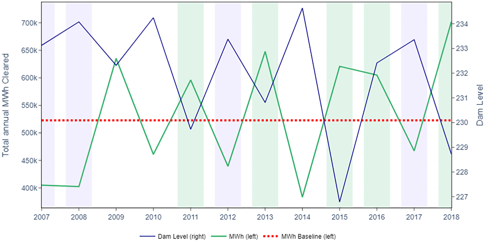
Figure 2 presents aggregate annual hydroelectric production in the NEM from 2007 to 2018. Although an ideal research design will examine production patterns before and after the introduction of the RET, our sample is restricted for reasons explained in section 5.1. Of most significance is the fact that Tasmania’s power stations were only connected to the NEM in late 2005. 15 This is important as several of Australia’s hydroelectric plants are located in Tasmania. The other significant event for hydroelectric production was Australia’s Millennium drought which peaked between 2007 and 2009. Aggregate hydroelectric production is depressed over this period. From 2009 onwards, there is significant year on year variability in annual hydroelectric production across the entirety of the NEM. This trend implies that there are factors that lead hydroelectric power stations to vary their year-on-year production decisions. We are interested in whether this year-on-year variability is the product of natural factors such as the weather and wholesale market conditions, or if the baseline method for awarding RECs to pre-existing facilities is contributing to this variation.
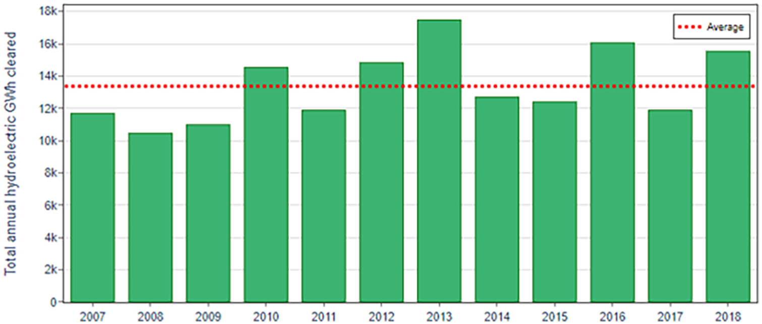
Annual hydroelectric energy generated in the NEM.
Figure 3 presents annual hydroelectric production for Tasmania’s John Butters Power Station between 2007 and 2018 against the baseline that applies to the facility. For John Butters, annual volatility in production observed in Figure 2 persists at the station level. We see that low output years are associated with rising dam levels, which are then followed by high output years above the station’s baseline level. Even in years where output is closest to the baseline, production levels rarely come within 10 percentage points of baseline levels.
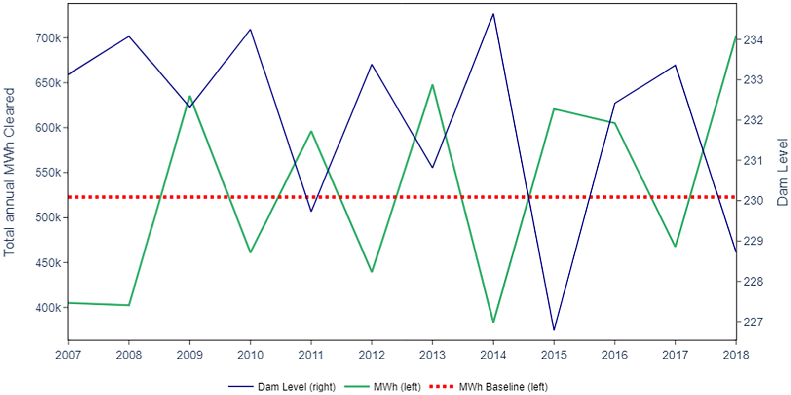
Annual hydroelectric energy generated by John Butters Power Station.
Figure 4 presents John Butters daily MWh generated for the last and first month of each year from 2009 to 2018 (excluding years impacted by the Millennium drought). The REC formula resets each calendar year, where RECS are only awarded for annual production within that year that exceeds the facility’s baseline. Therefore, if the RET is distorting annual production decisions, we would expect to observe a change in production behavior around the beginning and end of each calendar year since that is the administrative reset date. While there are no abrupt discontinuities for this facility, there are several years with either a relative increase or decrease in production behavior. For example, in 2010 to 2011, 2014 to 2015 and 2017 to 2018 we observe increases implying that the station may be entering a REC year. Conversely, in 2009 to 2010, 2015 to 2016 and 2016 to 2017 we observe decreases, implying that a station may be entering a Storage year. In most cases, this change in behavior coincides with high and low output years observed in Figure 3.
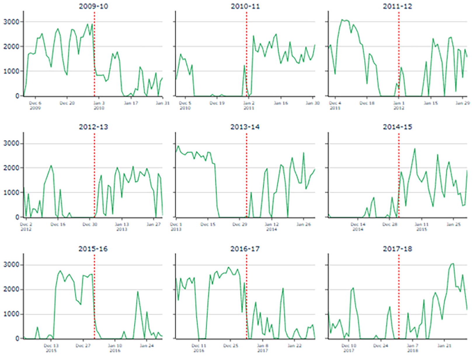
Hydroelectric energy generated by John Butters Power Station in RET year transition periods.
These observations demonstrate that annual variation exists, and has done so for the decade or so prior to 2018. Figure 4 also suggests that a hydroelectric plants decision to alter annual production may align with the administrative definition of a year in the context of the REC formula. To understand whether the baseline method contributed to this variation we define a simple theoretical model of a hydroelectric firms production problem with and without the RET as it applies to pre-existing units. Motivated by this theoretical model, we then conduct an empirical exercise examining hydroelectric production in the NEM.
4. A Conceptual Framework for Hydropower Economics
In this section we give attention to the production incentives for hydroelectric firms. Hydroelectric energy is generated when water is channeled through turbines that drive an electrical generator. The amount of energy generated is influenced by (but not limited to) gravity, the height from which the water falls (head), the flow that can be achieved and turbine efficiency. 16 Because hydro-gravity power stations have the ability to store water in dams, their production decisions entail forward-looking elements. Using water for production today leaves less water in the dam tomorrow, with the expected additional benefit from having a higher dam level representing the opportunity cost of generation (Førsund 2015). The dynamic nature of their production decisions means hydroelectric output varies with factors beyond current electricity prices (Førsund 2015) – for example if price levels are expected to increase in the future, then the opportunity cost of using water today increases. Further the treatment of pre-existing hydro facilities under the RET could also incentivize year-to-year distortions in production observed in Figures 2 to 4. Recall, if a power station has a baseline of 1,200 MWh, then producing 1,000 MWh (Storage year) in one year and 1,400 MWh (REC year) in the following year grants them 200 RECs. Conversely, producing 1,200 MWh in both years grants them zero RECs. The remainder of this section formulates this production problem. In doing so we draw on the two-period bathtub model developed by Førsund (2015).
4.1. Hydroelectric Production Problem (Without the RET)
The stylized model of hydro operation we present includes numerous simplifications and a baseline of symmetric year-to-year conditions. This is to demonstrate the impacts of introducing a RET that allows pre-existing units to earn RECs for annual output that exceeds their baseline – a non-manipulable value equal to the historical, pre-RET, average.
The simplified physical assumptions include, for example, the absence of evaporation or replenishment, and the absence of broader water network considerations or regulatory water targets. The economic assumptions allow for a clear depiction of the incentives the operator faces: First, the marginal wear-and-tear cost of production is assumed to be zero; second, prices for all periods are known and follow the same distribution each year and third, producers are price takers. It has been specified with annual intervals containing hourly sub-periods to later demonstrate the specific implications of the REC rules in Australia.
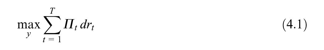
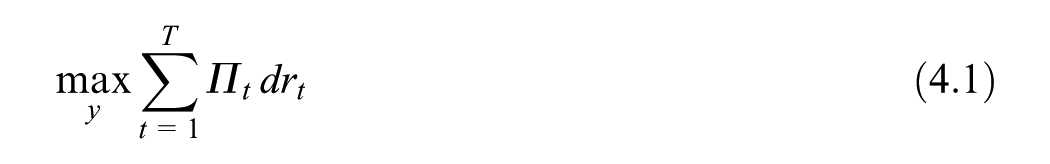
With this backdrop, the hydroelectric production problem is to maximize profit subject to a resource (water) constraint. We consider the following profit function:
Objective
where
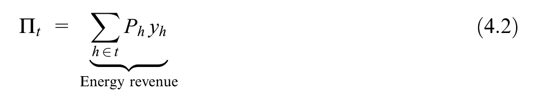

subject to

Equation (4.1) imposes that the hydroelectric plant maximizes profit (
For demonstration purposes, Figure 5 presents this production problem as a simple two-period bathtub model (T = 2), with
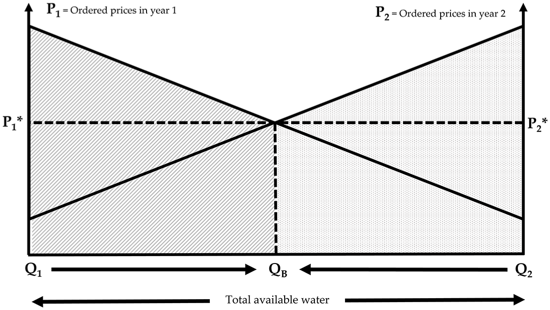
Hydroelectric production problem over two periods (years).
This stylized model demonstrates the dynamic nature of hydroelectric production decisions. Consider if the hydroelectric plant were to deviate from
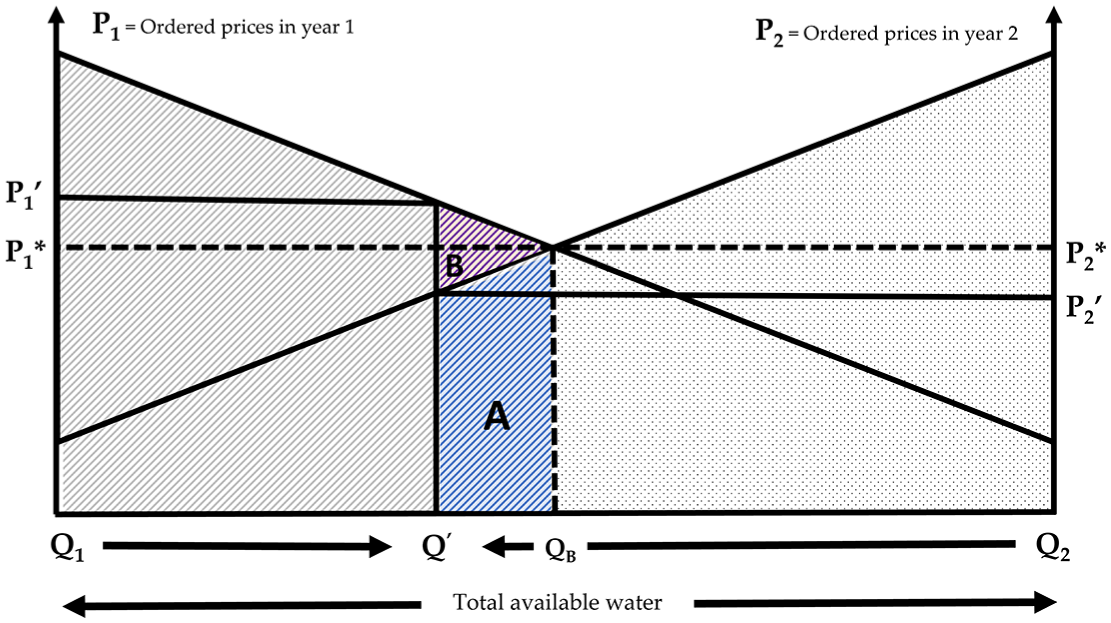
Effect of a change in hydroelectric production over two periods (years) on firm profits.
4.2. Hydroelectric Production Problem (with the RET)
The presence of the RET alters the hydroelectric production problem. With the possibility of generating REC revenue, the profit function is reformulated as:
Objective
where
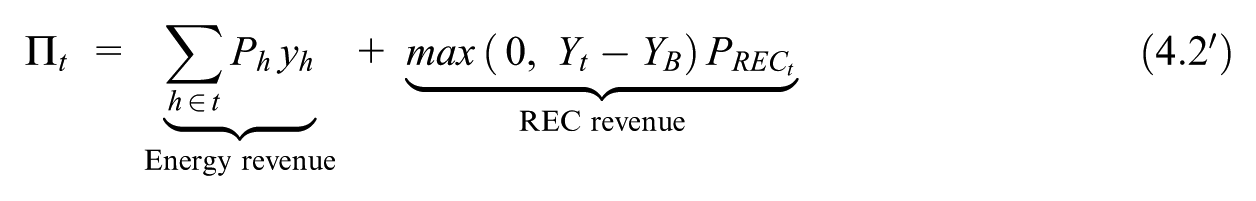

subject to

Equation (4.1) remains unchanged. Similarly, equation (4.3) and our constraints remain unchanged. However, our profit function in equation (4.2) is replaced by equation (4.2’) which now includes a function that seeks to maximize the revenue generated from REC production above a station’s (non-manipulable) baseline (
Figure 7 replicates the simple two-period bathtub model presented in the previous section for this new production problem. Consider the case where
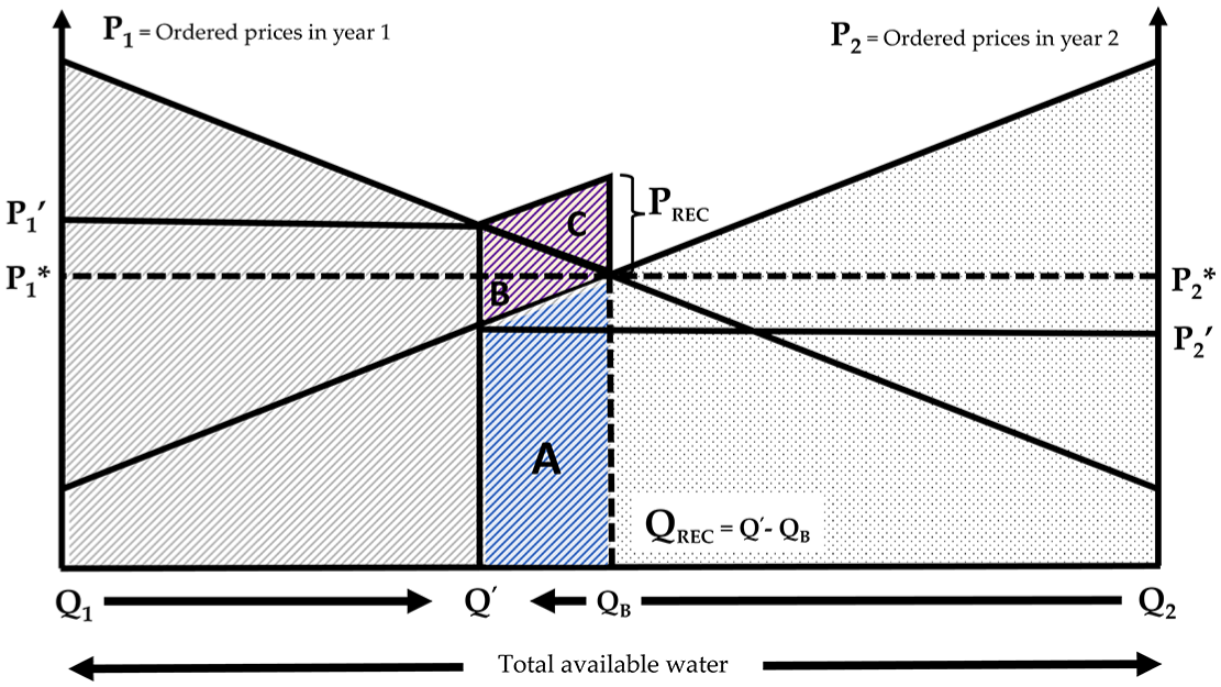
Effect of a change in hydroelectric production with RECs over two periods (years).
5. Data
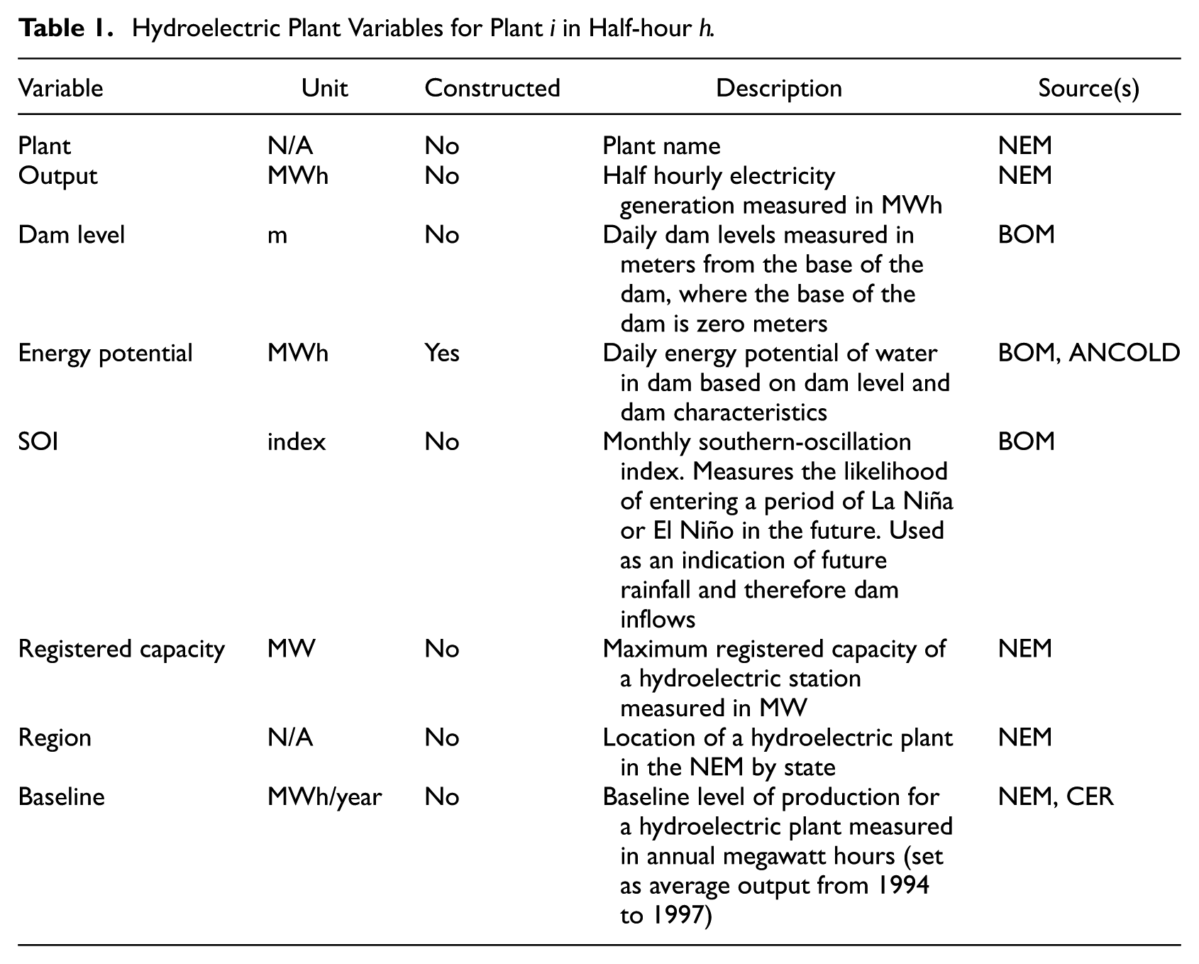
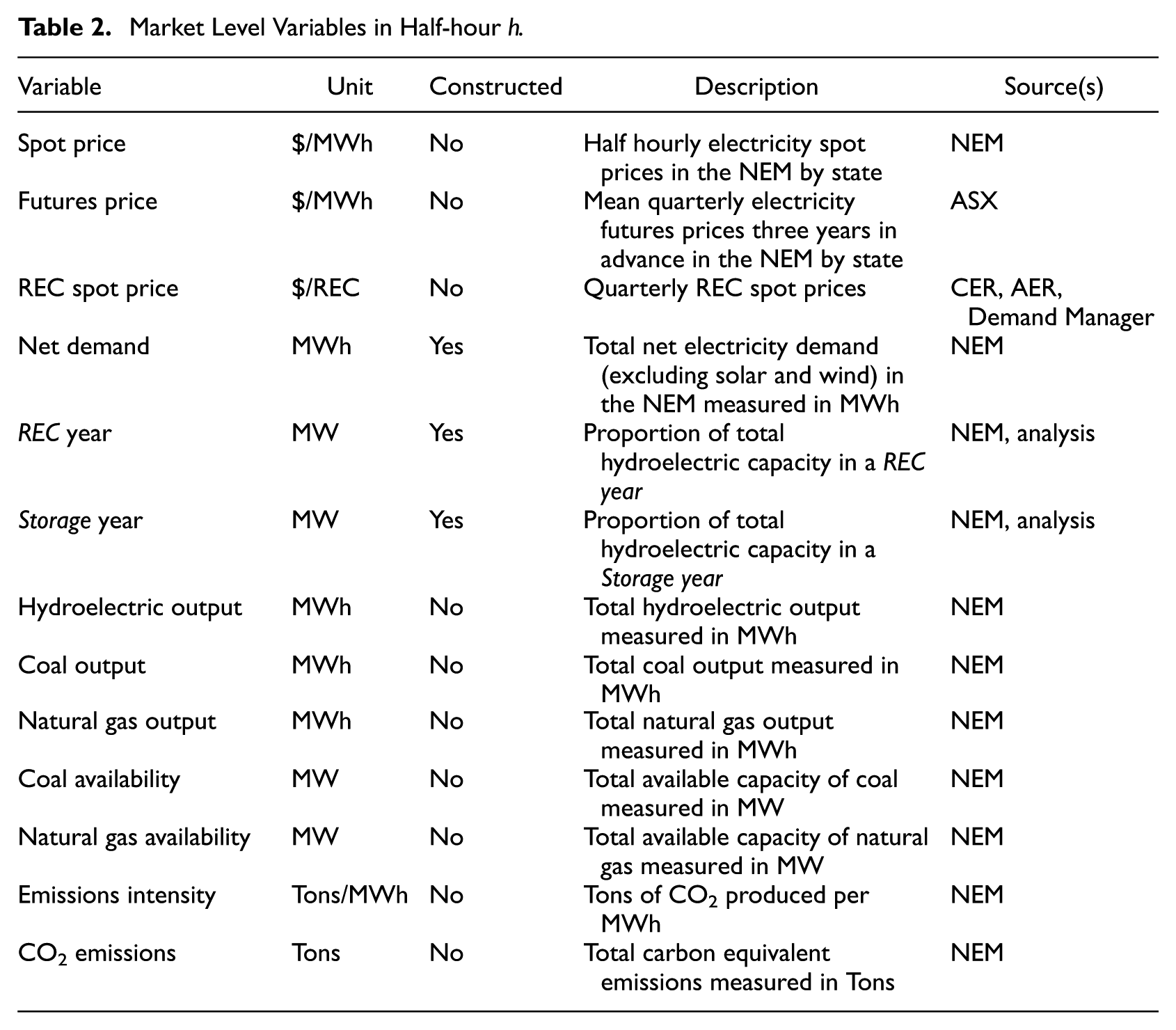
We combine half-hourly electricity market output and price data with daily hydrological data, plant characteristics, and REC price data from 2007 to 2018. An ideal analysis would commence pre-RET; however the analysis period is determined by available data – the RET was introduced adjacent to the introduction of market-based electricity dispatch in Australia, with operational data pre-NEM not available. Data availability and constraints are outlined explicitly in Section 5.1. For the first stage of our analysis, data is collected and analyzed at a plant level. For the second stage electricity output data is aggregated by fuel source and analyzed at a market level. The main sources of data include the NEM, Australian Energy Market Operator (AEMO), Australian Energy Regulator (AER), Clean Energy Regulator (CER), Bureau of Meteorology (BOM) and Australian National Committee on Large Dams (ANCOLD) database. Each dataset has varying levels of completeness and reporting frequency. To overcome these limitations, for some variables we backfill between observations. For example, dam levels are only reported once daily. We therefore adopt the same dam level for all half-hourly periods in that day. For others, we construct the variable based on other observed variables. Tables 1 and 2 indicate whether a variable was constructed. Variable construction is outlined in Appendix A1.
Hydroelectric Plant Variables for Plant
Market Level Variables in Half-hour
5.1. Data Availability and Analysis Period
We compile datasets for twenty-two of Australia’s forty-nine hydroelectric gravity plants. Seventeen plants were omitted as they are mostly inactive and therefore did not have consistent output data. For a further five plants, BOM did not capture data on dam levels. Finally, in a small number of instances, separate plant names shared the same NEM identifier and were therefore combined and considered the same plant. Importantly, the twenty-two plants captured in our analysis are responsible for roughly 75% of registered hydroelectric capacity in the NEM and include all of Australia’s hydroelectric plants with an overall capacity greater than 50 MW. Our analysis period is determined by several factors. Tasmania contributes a large proportion of the NEMs hydroelectric capacity but was only connected to the NEM in 2005. Incomplete datasets for several key variables, including REC prices, and dam levels, leaves a balanced panel from 2007 to 2018.
5.2. Hydroelectric Plant Data
To analyze the effects of the RET on hydroelectric production we collect data on electricity production, dam storage levels, hydroelectric plant capacity and other plant characteristics, and finally RET production baselines. We also utilize the Southern Oscillation Index, which relates to projected seasonal rainfall. Table 1 outlines plant-level data used in our analysis.
5.3. Electricity Market Data
Both stages of analysis rely on electricity market data. We collect data on electricity market prices, electricity production by fuel type, emission intensities, electricity demand and available capacity by fuel type. Market data, including units and timestamps, is outlined in Table 2.
6. Empirical Approach
Our analysis contains two parts. First we empirically classify year-to-year production distortions among Australia’s hydroelectric plants. Second, we examine the market level spillovers from these distortions. Each stage requires its own empirical approach. The remainder of this section is focused on detailing these approaches. The results for each stage are presented and discussed in Section 7.
6.1. Analyzing the Effect of the REC Formula for Pre-existing Units on Hydroelectric Production Decisions at the Plant Level
We first describe how we classify high and low hydroelectric output years that are not being driven by weather and wholesale market conditions. To do this we estimate a descriptive linear model of hydroelectric production on a plant by half-hourly dataset. Using the outputs of this model we establish a classification algorithm that identifies when output is significantly different from mean levels for each hydroelectric plant conditional on market and weather conditions present in that year. We refer to years with uncharacteristically high levels of production as REC years, and years with uncharacteristically low levels of production as Storage years. These are years in which hydroelectric output is most likely being distorted by the RETs vintage differentiated baseline. We verify our classifications by observing changes in daily output on days either side of the RETs administrative reset date of January 1.
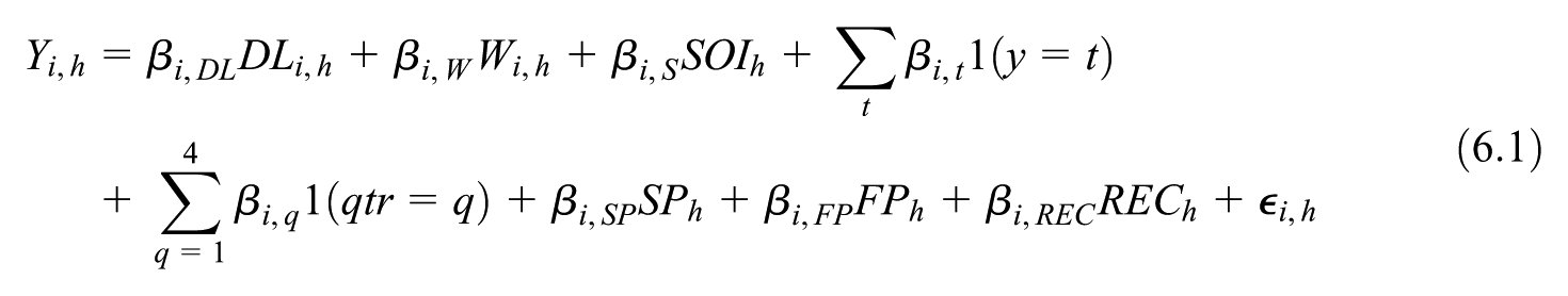
Modeling Hydroelectric Production
Equation (6.1) describes plant-level production as a function of known profit drivers for each hydroelectric plant. This linear function includes wholesale market prices, weather conditions and renewable energy certificate prices. Estimating this model returns a best linear predictor function for plant-level output over our sample window. The nature of this model is descriptive, with coefficients not having a causal interpretation.
The purpose of this model is to identify whether there is unexplained year-to-year variation that aligns with administrative REC years that are not captured by variation in the profit drivers of hydroelectric dams. To do this, we estimate the model without a constant and instead includes a fixed effect for each year
Model
Where
Classifying REC and Storage Years
We interpret variation in the year fixed-effects
1. Calculate the mean year-fixed effect for each hydroelectric plant:

2. Subtracting

Because our regression measures hydroelectric output in megawatt hours,
Low thresholds classify more years, and high thresholds less. We take a data-driven approach to select the threshold that best fits our market-level model. Given that equation (6.1) is estimately separately for each facility, we use a method that chooses the threshold that maximizes the market-level fit of the data, which is described in the next section. Specifically, we select for the threshold that minimizes the mean squared error of equation (6.3) (see Section 6.2) on hydroelectric output. This process defines a threshold as

In summary, having controlled for the main factors that influence hydroelectric output, we classify a plant
Verifying the Classification of REC and Storage Years: Hydroelectric Output (Dis)continuity at Administrative Reset Dates
To verify whether hydroelectric plants are in fact adjusting output in accordance with our REC and Storage year classifications, we analyze daily hydroelectric output levels at the beginning and end of each calendar year. As mentioned, the RET only awards RECs for production in a given calendar year. If the REC formula for pre-existing units is distorting production decisions, we should expect to observe a change in output behavior either side of the January 1 threshold. Equation (6.2) specifies the fixed-effects model used to estimate average daily output
Model
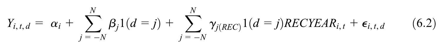
Where
6.2. Analyzing the Effect of the REC Formula for Pre-existing Units on the Composition of Energy Production at the Market Level
After classifying REC and Storage for each plant, we move to analyzing market-level measures of output.
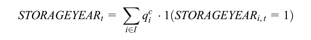
Creating Market Level REC and Storage Year Variables
To understand market-level effects of hydroelectric plants likely amplifying their annual production in response to the incentives under the methodology for awarding RECs, we first have to aggregate the results of our REC and Storage year classifications. The spillover effect of a given hydroelectric plant entering a REC or Storage year depends on the size of that plant. For example, in a REC year, a small plant would produce far less energy than a larger equivalent. Hence, we weight each plants REC and Storage year classification according to its NEM registered capacity

Determining the Effect of the REC Formula for Pre-existing Units on Output and Emission Levels for Different Fuel Sources
Equation (6.3) models market-level output for various fuel sources in the NEM as a function of market demand, fuel availability and the REC and Storage year variables defined above. This allows us to examine whether our classification of REC and Storage years are correlated with the market-wide output of different fuel sources, including aggregate hydroelectric output. Through the same process, we examine their correlation with on net carbon equivalent emissions. We estimate our model using ordinary least squares with HAC standard errors.
Model

7. Results and Discussion
To align with our two-part method, sections 7.1 and 7.2 present our results as two discrete but complementary sections. Section 7.3 discusses the robustness of our results. Finally, section 7.4 considers policy implications.
7.1. Hydroelectric Production Decisions at the Plant Level
Here we present our REC and Storage year classification and verify whether the classification is being driven by the REC formula for pre-existing units. This discussion reflects the combined outputs of equations (6.1) and (6.2).
REC and Storage Year Results
Figure 8 replicates Figure 3 with the results of our REC (green) and Storage (blue) year classifications as shaded columns for John Butters power station. As hypothesized, we observe a pattern of low output Storage years, followed by high output REC years. We observe mostly similar results for the twenty-one other hydroelectric plants included in our analysis – namely that low output, high storage level years are classified as Storage years, and are generally followed by high output years that get classified as REC years. Estimated parameter values from equation (6.1) that inform these classifications are presented in Tables A1 and A2 of Appendix A2.
REC and storage year classifications for John Butters Power Station.
Despite the prevalence of REC and Storage years in Figure 8, there are three years which are not classified as either REC or Storage years. These years are of interest because they imply something about the robustness of our classification algorithm. For example, despite not being classified, 2010 has some of the characteristics of a Storage year. However, when also observing spot prices in 2010, we see that NEM spot prices were at their lowest point over the entire analysis period. Given such conditions, our classification algorithm interprets output levels in these years as normal. 2010 therefore reflects a year in which, given weather and wholesale market conditions, output was neither abnormally high nor low. This provides confidence that the classification algorithm is reasonably performing the descriptive exercise to distinguish between unclassified, REC, and Storage years. Further we note what looks to be often a year-to-year swing in production from REC to Storage year with the exception of 2015 to 2016. 2016 was the fifteenth wettest year on record in Australia, allowing for generation levels to remain high while also seeing storage levels increase.
While compelling, these results do not guarantee that the REC formula for pre-existing units is the cause of observed yearly swings in output. They only suggest that there is some unknown factor that is reliably altering year-to-year production. To further verify our hypothesis we narrow our focus to the period either side of the RET reset date.
Verifying Our REC and Storage Year Results: Administrative Deadline Discontinuities
If the REC formula for pre-existing units is the cause of distortions, we should expect to observe a change in output behavior either side of its January 1 reset date for earning RECs. Other than representing the reset date for earning REC certificates, January 1 has no significance for a hydroelectric plants output decisions. We consider estimates from equation (6.2) around the January 1 RET reset date for three scenarios:
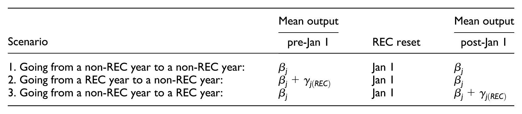
If the REC formula for pre-existing units does not impact production decisions, we expect the
Model results are presented in Figure 9 and Table A3 of Appendix A3. Figure 9 presents estimates for our three scenarios of interest. Panel one reflects scenario 2 and Panel two reflects scenario 3. Scenario 1 is not explicitly presented but is simply the combined Non-REC year results across both panels.
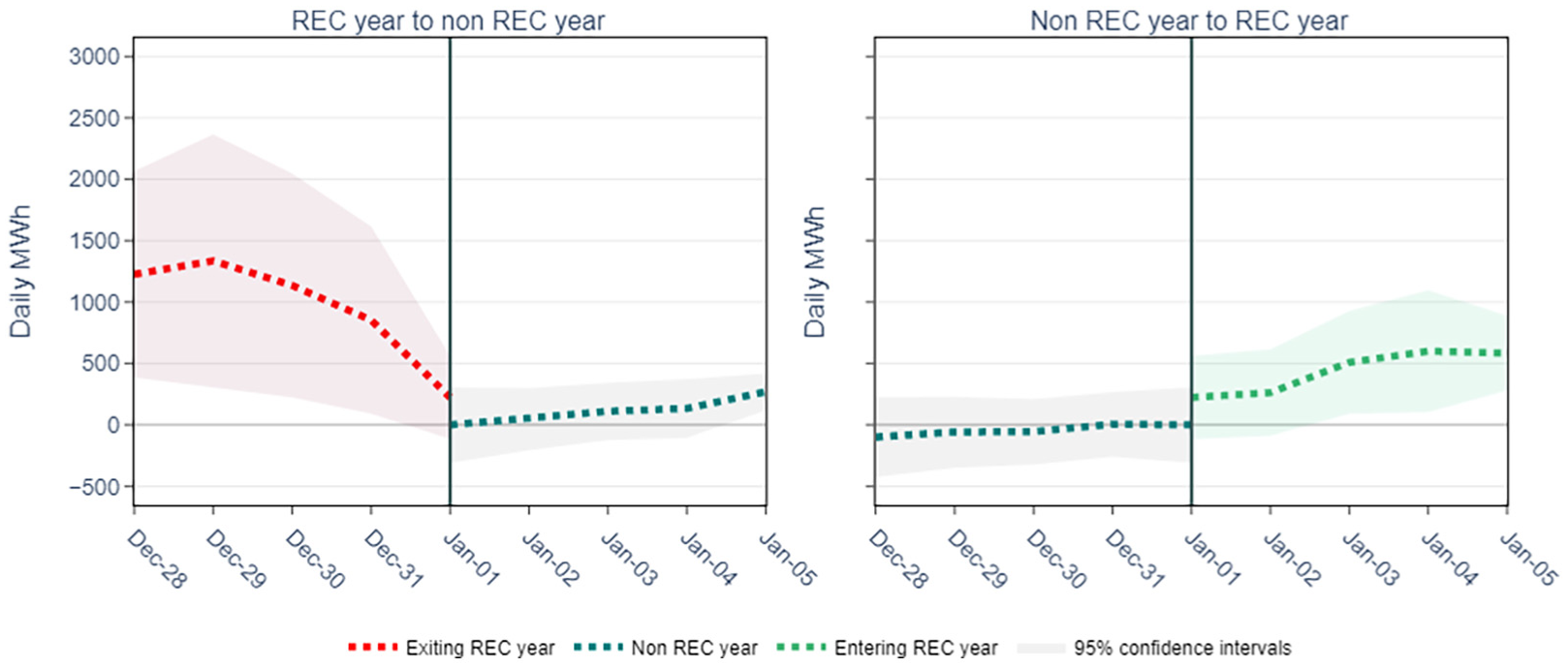
Average daily output for NEM hydroelectric plants either side of the RET reset date.
We see REC year output is on average higher than non-REC year output on days either side of the REC administrative year reset date
Overall these results are in support of the impacts suggested by the stylized model – hydroelectric plants are responding to the design of the RET where they only receive RECs on output that exceeds their baseline in a given year. The fact that we observe abrupt changes in output across firms around a narrow window either side of the RET reset date further reinforces this hypothesis.
7.2. Effect of the REC Formula for Pre-existing Units on Market Level Production and Carbon Emissions
We extend our results from section 7.1 to examine whether our classification of REC and Storage years has predictive power for market level production for different fuel sources. Table 3 presents the outputs of equation (6.3) for four dependent variables – hydroelectric output (column 1), coal output (column 2), natural gas output (column 3) and carbon equivalent emissions (column 4). These results examine whether our REC and Storage year classification are correlated with the composition of fuel types in the market, and equivalently net carbon equivalent emissions. We include p-values for a joint hypothesis test that determines whether the model predicts that the net impact of a REC year followed by a Storage year is zero. If zero, this implies that there are no net production distortions when aggregated across multiple years – or that average production over a two-year horizon for a given fuel source is not predicted to differ if hydro facilities enter a storage year that is followed by an equivalent REC year.
OLS Results for Half-hourly Output (MWh) by Fuel Type and Carbon Equivalent Emissions (Tons).
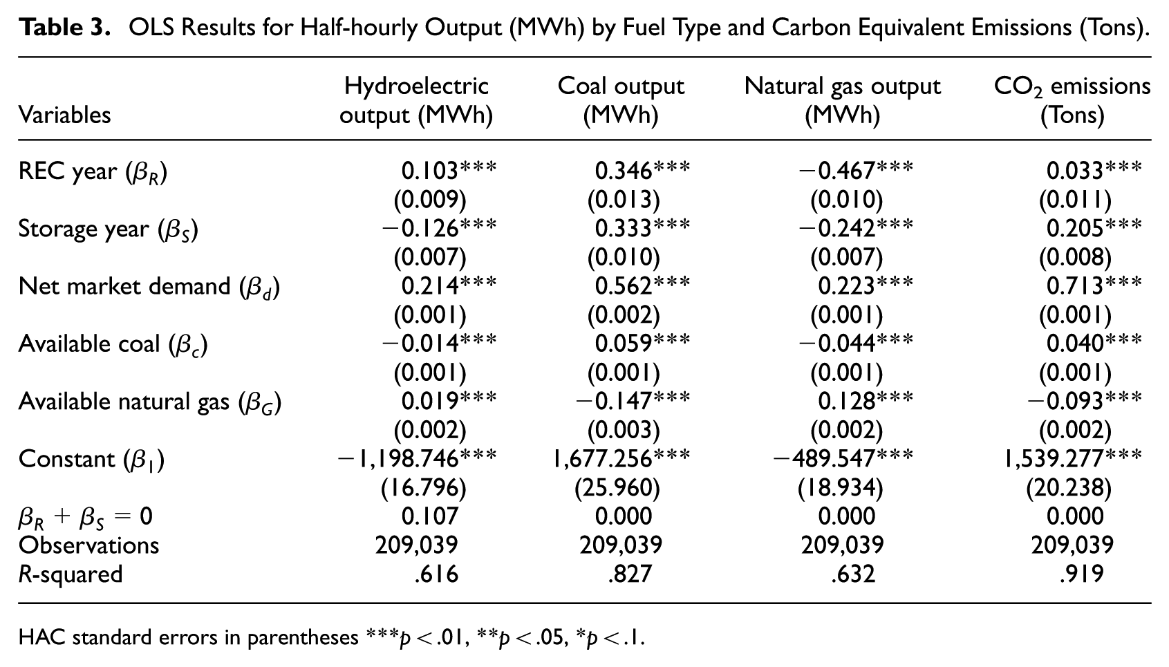
HAC standard errors in parentheses ***p < .01, **p < .05, *p < .1.
Effects on Hydroelectric Production
As expected, we observe in column 1 of Table 3 higher aggregate hydroelectric output in REC years relative to Storage years. Specifically, our model predicts that for every additional MW of registered hydroelectric capacity in a REC year, half-hourly hydroelectric output in the NEM is on average 0.103 MWh higher. Conversely, for every MW of registered capacity in a Storage year, half-hourly output is predicted to be on average 0.126 MWh lower.
22
Hypothesis tests for the REC and Storage year coefficients being zero are rejected at a 5% level. The observed swings in market level hydroelectric output when entering either a REC or Storage year are almost the inverse of one another. We formally test and cannot reject the joint hypothesis test that
Because of the structure of energy markets, we should expect to observe these changes in production being offset by a roughly equivalent change in production from alternative fuel sources. Hence these year-on-year variations are likely to have spillover effects in the rest of the market (Archsmith 2022; Eyer and Wichman 2018).
Effects on Fossil Fuel Production
To understand how the RET’s baseline treatment of pre-existing hydro facilities might spill over to fossil fuel production, we observe how the output by coal (column 2) and natural gas (column 3) vary across REC and Storage years throughout our sample. Somewhat surprisingly, half-hourly coal output on average was 0.346 MWh higher with every additional MW of hydroelectric capacity in a REC year during our sample period. The corresponding figure for natural gas output is 0.467 MWh lower. These results make more sense when observing changes in REC year output across all three fuel types. Combined increases in half-hourly hydroelectric and coal output (0.449 MWh) are roughly offset by the predicted decrease in half-hourly natural gas output (0.467 MWh).
In Storage years, this pattern is inverted. Half-hourly coal output on average was 0.333 MWh higher with every additional MW of hydroelectric capacity in a Storage year during our sample period. The corresponding figure for natural gas output is 0.242 MWh lower. This represents a net increase in half-hourly fossil fuel output of 0.091 MWh, proximal to the 0.126 MWh decrease in half-hourly hydroelectric output in a Storage year. Despite observed decreases in natural gas output, output levels for natural gas are higher in Storage years relative to REC years. Coal output is actually slightly lower in Storage years. However, this decrease is small, with net output coming from fossil fuels in Storage years increasing. This gives rise to the possibility that the substitution patterns between fuel sources may be emissions-increasing.
For both coal and natural gas output, we reject the joint hypothesis test that
Effects on Carbon Equivalent Emissions
Our results so far imply that, through distortions to hydroelectric production incentives, the REC formula for pre-existing units may increase output coming from fossil fuels and by extension carbon equivalent emissions. Column 4 of Table A1 presents these results. We see that carbon equivalent emissions on average were higher during our sample in both REC and Storage years. However, the magnitude of this increase is far greater in Storage years when hydro generates less energy. Our model predicts that half-hourly carbon equivalent emissions increase by 0.033 and 0.205 tons for every MW of hydroelectric capacity in a REC and Storage year respectively. These results are unsurprising in the context of the observed changes in fossil fuel output in a Storage year. That is, we expect carbon emissions to increase with increased net output coming from fossil fuels. Our REC year results are somewhat surprising given the net decrease in output coming from fossil fuels in these years. However, the composition of this change is important. While net fossil fuel output was lower in REC years, output coming from coal was higher. In general, the emissions intensity of energy from coal is approximately 0.3 tons per MWh higher than natural gas. Hence the decrease in emissions coming from natural gas appears to be outweighed by the increase in emissions coming from coal.
We now stretch the interpretation of this exercise in an attempt to demonstrate the potential magnitude the REC baseline incentives might have on carbon emissions. Assuming hydroelectric plant operations conform to our REC and Storage year predictions, if all hydroelectric plants were to simultaneously transition from a REC year to a Storage year, our model predicts that substitution patterns result in a net increase in half-hourly carbon equivalent emissions of 510 tons, or an increase of roughly 24,500 tons per day. Assigning a social cost to carbon equivalent emissions of $50 per ton, this equates to incremental damages of roughly $1,225,000 per day above a counterfactual scenario where production is not being distorted. We stress this is not a counterfactual grounded in a microfounded model of energy production, rather a demonstration that any subsequent substitution effects from distorting year-on-year hydro production may be meaningful.
Consistent with findings by Archsmith (2022) our results suggest that suboptimal policy design can create inefficiencies in the subsequent markets that hydro generators participate in, resulting in unintended social costs. The true social cost of the inclusion of pre-existing facilities in Australia’s RET, which incorporates its impact on carbon equivalent emissions, is uncertain, but we demonstrate the potential for emissions to increase. Further, our paper only focuses on the spillovers to energy markets from this treatment of pre-existing facilities in the RET. There is also the potential for spillovers to irrigators and the environment in downstream locations. Finally, this is not a holistic policy evaluation of the RET, as the program promoted significant development of new wind and solar resources (Nelson et al. 2022).
7.3. Additional Specifications
As outlined in Section 6.1, there was discretion over the threshold used to classify REC and Storage years in the results presented above. We ultimately took a data driven approach to derive a value that minimized the mean square errors of equation (6.3) (10% threshold). Results show that 6% and 12% threshold provide local minima and are the next best fit for thresholds. We test the sensitivity of our results to this threshold by observing how they change under different specifications. For completeness we replicate our analysis using both the 6% and 12% thresholds. The results for these thresholds are presented in Tables A4 and A5 of Appendix A4.
The relative pattern of results in Table 3 do not change under the 6% and 12% thresholds, their relative magnitudes just change slightly. We still observe higher hydroelectric output in REC years and lower hydroelectric output in Storage years. To offset these values, we observe increases in coal output and decreases in natural gas output, with net carbon equivalent emissions increasing in the transition from a REC year to a Storage year.
7.4. Policy Implications
Awarding RECs to pre-existing hydroelectric plants can return windfall gains for these hydroelectric plants, all else held equal. Importantly, when considering the counterfactual behind this claim, it requires carbon, the externality motivating the introduction of a RET, to remain unpriced. If instead the counterfactual is a world with carbon pricing in a fossil-dominated grid like Australia’s, electricity prices, and thus hydro profits, would be higher in the carbon tax world.
These gains to pre-existing plants under the RET represent a cost to consumers through increased electricity prices and are essentially a transfer of wealth. While undesirable to consumers, windfall gains are often observed in transitional policy arrangements (Bergek and Jacobsson 2010; Fraser et al. 2023), and often viewed by policymakers as politically necessary to pass reform (Stavins 2005). This is not an observation on the overall consumer and welfare impacts from the RET, which includes emission and market impacts, following from additional new renewable energy investment (see Nelson et al. 2022, for further discussion). Rather, this comment relates specifically to the treatment of pre-existing plants under the RET.
The design of the REC allocation to existing hydroelectric dams impacts their operating incentives. This can be accompanied by economic impacts beyond wealth transfers. Because of the nature of electricity markets, these incentive distortions are having spillover effects in the rest of the NEM. This reallocation of production may even lead to an increase in carbon equivalent emissions when compared to a world where pre-existing plants are not included under the scheme – an outcome that is the antithesis of the RET. Our analysis demonstrates that the non-linearity in the REC accrual rule for hydroelectric generators, that might appear to be sensibly based on historical yearly production averages, has the potential to deliver unintended (and often unobserved) social costs.
Removing the baseline methodology for pre-existing plants is likely to improve the efficiency of the policy. However, if inclusion of pre-existing plants into a RET is deemed necessary, we discuss several approaches that will remove or diminish the year-on-year distortionary incentives the existing baseline approach provides.
The first is to award RECs to pre-existing hydroelectric plants for their entire output in a given year. While this would remove the incentive to distort production, it is unlikely to be viewed as equitable. However, one may take the view that introducing a carbon tax, the first-best approach to addressing a carbon externality, is the most relevant counterfactual to consider and also introduces a windfall to pre-existing renewable energy resources. Carbon taxes are passed through to higher wholesale electricity prices as fossil-fueled plants experience an increase in their operating costs, resulting in higher profits to hydro plants. A zero-baseline approach to awarding RECs will provide incentives for pre-existing plants equal to new renewable plants to perform operating, maintenance and investment/expansion decisions to increase their lifetime energy production.
A similar approach is seen with the UK’s Renewable Energy Guarantees of Origin (REGOs). 23 Although these are not surrendered under a regulated scheme to achieve a RET, they treat all output from renewable resources equally, regardless of vintage. To the extent REGOs hold value (to allow “clean” energy retailers to certify their procurement), this equal treatment across resources does not incentivize distortions in year-to-year output patterns by hydro operators.
The second is to consider any capacity expansion of pre-existing plants in a bespoke manner. That is, pre-existing plants can only gain entry to the scheme following a credible expansion in lifetime energy capacity. In this case, for a large enough expansion, a baseline approach may be less susceptible to year-to-year distortionary operating incentives if the expansion means the whole facility always exceeds annual baselines and consequently has no incentive to shift output across years to maximize their creation of RECs. For example, the Arizona RET (coined a Renewable Portfolio Standard, or RPS), allows pre-existing hydro facilities to enter the scheme if they have increased their capacity. 24
Finally, numerous US States apply different credit multipliers or carve-outs within their RPS certificate schemes based on the generation technology (Lips 2018). Many credit multiplier amendments to RPS/RET schemes are predicated on promoting newer technologies, or to achieve other state and community priorities. In principle, pre-existing generating assets can be subject to no output baseline, but instead receive a discounted credit multiplier on their output for certificate creation purposes. Although this would reduce the large gains to pre-existing resources relative to full inclusion to a REC scheme, it also mutes their incentive to improve their lifetime output if they are permanently subjected to a reduced multiplier. We do not offer an economic rationale for applying different multipliers to pre-existing resources, we simply note that such an approach would not incentivize distortions in year-to-year output patterns by hydro operators.
8. Conclusion
Policymakers introducing new policies or regulation need to decide if and how rules and requirements differ for existing and new entities. We demonstrate that the introduction of Australia’s Renewable Energy Target created significant changes to the operating incentives of existing hydroelectric generators. Plant owners receive a Renewable Energy Certificate for every MWh generated beyond their historical yearly average output. This creates a nonlinearity in their profit function that incentivizes annual fluctuations in output – storing additional water one year, and then generating additional output the next. Empirically, we see plants often generate in ways consistent with this pattern, which is made more stark at the administrative REC year deadline.
This design may have resulted from real or perceived political necessity in order to pass reform, or may have been an attempt to incentivize existing renewable energy facilities to increase their lifetime energy output in some manner. With many jurisdictions around the world considering ways to implement a clean energy transition, potential schemes will require explicit decisions whether and how to treat existing plants. We demonstrate that what might appear to be an innocuous and perhaps small benefit to existing clean energy plants can return significant changes in their operating incentives. These incentives then can result in changes to the allocation of production, which in turn can impact economic efficiency and perhaps even carbon emission outcomes that run counter to the intention of the policy. Although the impacts identified in this paper may be small relative to the overall impacts of the scheme, there are approaches to including pre-existing facilities to renewable certificate schemes without distorting incentives to increase year-to-year variation in output that may better achieve policy goals. This can include a more bespoke eligibility process, that examines whether operational or investment decisions have expanded the lifetime energy generating capabilities of a facility. This approach is seen in the Renewable Portfolio Standards of some U.S. State jurisdictions, where pre-existing facilities need to demonstrate changes to the technical characteristics of the plant to be eligible to earn certificates.
Other approaches, such as full inclusion in a scheme or applying differentiated certificate credit multipliers, can remove the year-to-year operating incentive distortions, but may have other drawbacks. For example, full inclusion may deliver windfalls to pre-existing schemes that policy makers wish to avoid, or fractional credit multipliers may limit the incentives to increase lifetime energy output relative to new facilities. This further demonstrates that any policy reform does not simply apply to a future state of the world – it cannot be implemented without consideration of the transitional period. This entails explicit rulings on the treatment of pre-existing plants, with careful consideration of these transitional rules needed to achieve the outcomes desired by policymakers.
Footnotes
Appendix A
Funding
The authors received no financial support for the research, authorship, and/or publication of this article.
Declaration of Conflicting Interests
The authors declared no potential conflicts of interest with respect to the research, authorship, and/or publication of this article.
1
In other jurisdictions names include Tradeable Green Certificates, Green tags or Tradeable Renewable Certificates.
2
For example, Multiple jurisdictions in the United Kingdom, European Union and United States operate some form of RET policy.
3
Environmental grandfathering is typically implemented to reduce the cost of a new policy on old or pre-existing units that need to reduce their impacts on the local environment, by excluding incumbents from full policy exposure. However, less attention has been given to grandfathering in settings where incumbents can actually benefit from being exposed to a new environmental scheme, such as a RET.
4
For example, a jurisdiction with a 20% renewable energy target will achieve this by requiring retailers to surrender twenty RECs for every 100 MWh sold to their customers, with non-compliance facing a financial penalty which will lead to an implicit ceiling price for RECs.
5
6
The comparison to a non-RET status quo makes this a windfall. This might not represent a windfall relative to a world with no RET but with a carbon price, and thus higher electricity prices in a fossil-fuel-dominated grid such as Australia’s.
7
That is, business-as-usual operations will result in 200 RECs in the wet year (1400–1200), but each additional MWh generated in the wet year where output already exceeds the baseline earns an additional REC. So (assuming it is technically feasible) generating 900 MWh in the dry year, using their storage to delay generating 100 MWh to result in a total of 1,500 MWh in the wet year, will return 300 RECs, or an additional 100 from business-as-usual.
8
9
10
See Leslie (2018); ![]() for other examples that examine fuel switching in the context of carbon pricing or shocks to fuel costs.
for other examples that examine fuel switching in the context of carbon pricing or shocks to fuel costs.
11
A power station’s baseline can change if data was incomplete, or any errors were made when originally calculating the baseline. A baseline may also be altered if a Federal policy impacts a power station’s ability to produce energy (Renewable Energy (Electricity) Regulations 2001 (Aus))
12
13
See the Renewable Energy (Electricity) (Large-scale Generation Shortfall Charge) Act 2000. If a liable entity fails to meet their RPP obligation, they must pay a non-tax-deductible shortfall charge of $65 per certificate. Because it is non-tax deductible it is considered to have an effective value of around $93 (![]() ).
).
14
15
Connection occurred in 2005 following construction of the submarine interconnector Basslink.
16
Maximum flow rate is dictated by the size of the turbine and storage volume.
17
Ordered price distributions represent the prices at which a plant sells different bundles of electricity within one period. For example, hourly prices within a year ordered from highest to lowest
18
REC prices tend to only show meaningful variation at a monthly to quarterly timescale and vary less than electricity prices.
19
We explicitly exclude a constant from our model so each fixed effect can be separately estimated and compared to the mean fixed-effect.
20
We use future prices one year ahead to align with the annual nature of the REC administrative formula for pre-existing units.
21
Coal is an umbrella term that captures brown and black coal output. Natural gas is an umbrella term that captures gas, diesel, oil and coal seam gas output.
22
Although these results are sensible in a directional sense, we reiterate the non-causal nature of this descriptive exercise when interpreting the magnitudes. The magnitudes predicted by the model suggest approximately a 20 percentage point change in the capacity factor of a single unit that enters a REC year, which is material. It compares with, for example, the annual capacity factor of