
Abstract
Using 5-minute locational marginal prices for approximately 16,500 locations in ERCOT over a 152-day period in the summer and fall of 2023, we find strong evidence of a merit order effect from increased wind and solar output. We also find that increased wind and solar output can affect the component of locational marginal prices arising from transmission constraints. Backing out thermal generation to accommodate increased solar and especially wind output made transmission constraints more likely to bind and, especially in peak periods, exacerbated the most severe transmission constraints. Growth in non-dispatchable capacity coupled with roughly constant dispatchable capacity thus has exacerbated operational problems arising from rapid load growth. At least one transmission constraint was binding for 78 percent of the periods in our sample. Transmission is most stressed during peak loads and least stressed under intermediate loads. Increased thermal generation generally alleviated transmission constraints, as did increased physical response capability.
Keywords
1. Introduction
The marginal costs of wind and solar generation are zero (or, with subsidies, negative). Adding them to the supply stack should displace higher marginal cost thermal capacity, resulting in marginal system output being supplied by a lower marginal cost generator. This is known as the merit order effect. However, transmission constraints and the need to maintain system stability can require higher marginal cost generation to be retained. Furthermore, binding transmission constraints directly affect locational marginal prices (LMP) in ERCOT, potentially obscuring the merit order effect. Such constraints have become more common in ERCOT as lines built to serve historical supply and demand patterns have become less suitable. Growth in population, per capita economic output, and electrification have spurred strong growth in electricity demand (load), and new generators often have not been well-located to serve that load growth. Furthermore, while increased weather-dependent generation has raised the need for dispatchable generation, new natural gas capacity has merely offset retirements.
ERCOT calculates LMP for thousands of electrical buses on the network at least once and sometimes several times every five minutes. After LMP are grouped by location, they are aggregated using a weighted average into hundreds of preliminary “settlement point” prices (SPP). The final SPP are derived by adding additional pricing components, including the Online Reserve Price Adders and the Real-Time Online Reliability Deployment Price Adders. 1 The SPP are further aggregated temporally into fifteen-minute intervals to yield wholesale market payments to generators from distributors and other buyers. Since the LMP reflect both merit order effects and operational constraints so also should wholesale market prices.
Although LMP and SPP are called prices, they do not equal the marginal cost to the system of meeting a marginal increase in demand or the marginal value to the system of a marginal increase in supply at each location. To begin with, they reflect supply bids from generators, which need not correspond to their marginal costs if the wholesale market is not sufficiently competitive. In addition, the transmission component omits marginal transmission losses. 2 Nevertheless, the ERCOT LMP analyzed in this paper reveal substantial information about the locations, causes, and effects of transmission constraints, the role of load forecasts in contributing to or alleviating them, and the effects of marginal changes in generation on system operation including, but not limited to, the merit order effect.
Sections 2 and 3 outline recent developments in ERCOT loads and generation capacity. Section 4 discusses the extensive literature on measuring merit order effects. Our main contribution to this literature lies in using data with higher temporal and geospatial granularity that also allows us to examine the effects of transmission constraints. We also test for endogeneity and find that it matters. Section 5 provides an overview of our data. The statistical analysis of LMP begins in Section 6 by focusing on causes of binding transmission constraints. Section 7 examines determinants of the “shadow price of power balance” common to all the LMP. This is where the merit order effect should be most evident. Section 8 examines the locations of buses most affected by binding transmission constraints. Section 9 examines changes in the cross-sectional distributions of LMP over time.
2. Recent Developments in ERCOT Loads
Strong population growth and economic expansion account for much of the growth in ERCOT load over the recent twenty years shown in Figure 1. Since 2002, average annual load has increased 2.2% per year, cumulating to almost 20 GW. Peak load, which acutely affects the need for flexible, dispatchable resources, increased by almost 30 GW. Since 2000, commercial sector demand (34% of 2022 load) has increased the most (by 66%). Electrification of oil and gas operations has been a source of industrial sector growth (30% of 2022 load). Electrification of home heating (61.5%), which is already significantly higher than the national average (39.8%), has been a source of residential sector (36% of 2022 load) growth. Growth in cryptocurrency mining, data centers, the adoption of electric vehicles (EVs), 3 and a drive to electrify energy use more generally, are set to ensure demand continues to grow. In the longer term, carbon capture and storage and the “green” hydrogen industry may further increase demand.
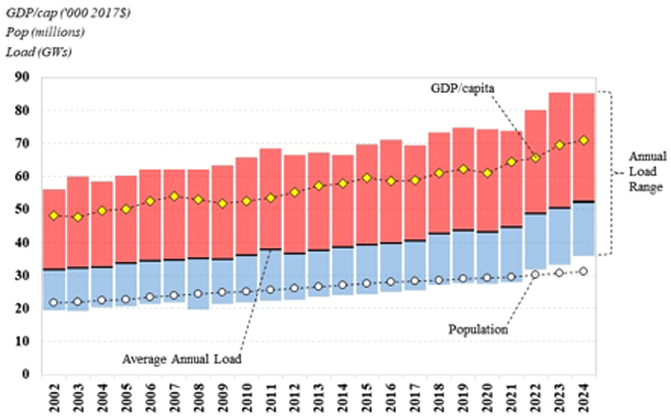
ERCOT load, Texas GDP per capita, and Texas population, 2002 to 2024.
The regional distribution of load growth helps determine transmission needs. Figure 2 disaggregates ERCOT into four load zones. The current official ERCOT load zones include four additional zones: Austin Energy, CPS Energy, Lower Colorado River Authority, and Rayburn Electric Cooperative. In our modified grouping (consistent with the data on forecasts we use later), Rayburn is included in the North zone, and the remaining three in the South zone. Figure 3 graphs monthly averages of hourly loads (sourced from ERCOT) in these zones from December 2010, when ERCOT officially transitioned to the current nodal market. Table 1 compares the zonal annual average and peak loads, and the hourly standard deviations of load in 2024 versus 2011.

ERCOT territory by modified load zone. 4
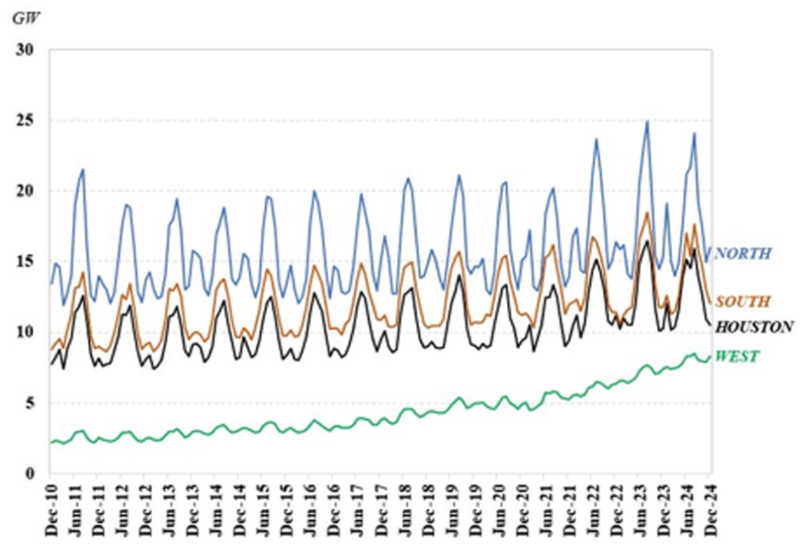
Monthly averages of hourly loads by modified zone, 12/1/2010 to 11/1/2024.
2011 Versus 2024 Load (in MW) by Modified Zone.
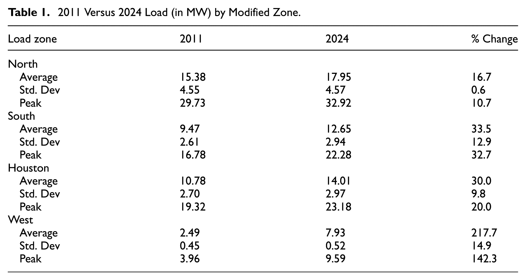
The North, South, and Houston zones have historically had the largest loads, but the West load increased by 218 percent from 2011 to 2024. This corresponds to rapid increases in oil and gas production in the Permian Basin coupled with efforts to electrify upstream operations, partly for environmental reasons. Load growth was second highest in the South zone, at 34%, and lowest in the North load zone, at 17%. Peak load growth, which critically affects the need for regional generation and grid resources, was closest to average load growth in percentage terms in the South zone.
3. Recent Developments in ERCOT Generation Capacity
As of summer 2023, the ERCOT generation portfolio totaled over 127 GW of nameplate capacity, categorized as natural gas (47.1 GW), wind (37.7 GW), solar (15.5 GW), coal (14.4 GW), nuclear (5.0 GW), and hydro/biomass/batteries (4.0 GW). In addition, there are DC ties (1.2 GW) to neighboring regions and natural gas capacity (3.7 GW) that is switchable between ERCOT and neighboring regions. Since 2000, the average annual growth rate of wind capacity exceeded 26% and of solar capacity exceeded 35% (Figure 4).
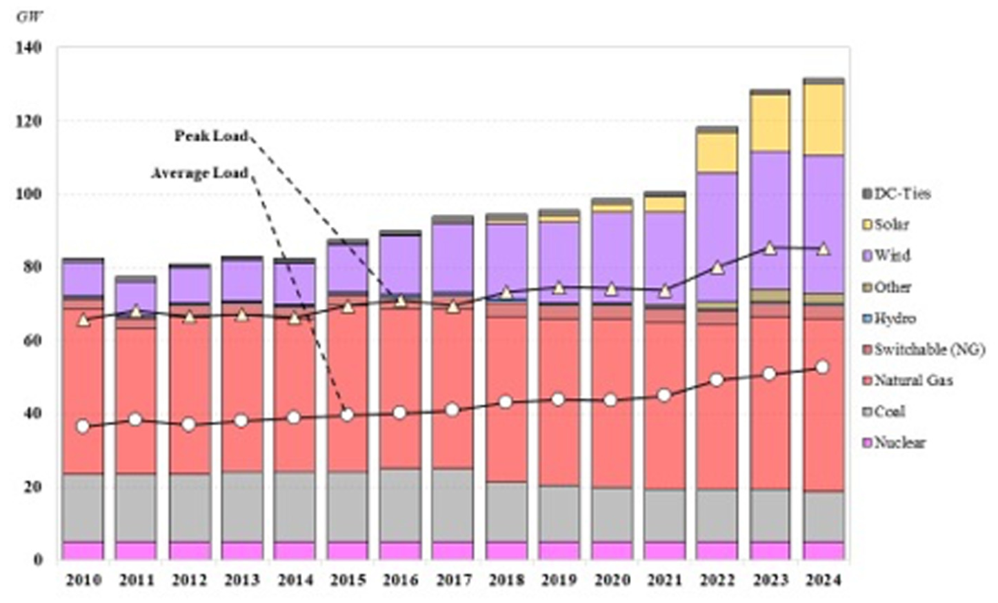
Generation capacity by type plus peak and average load, 2010 to 2024.
Average wind and solar outputs have increased in tandem with their capacities, but wind and solar often deliver well above or well below their monthly mean outputs. Moreover, wind and solar outputs are less complementary than Slusarewicz and Cohan (2018), for example, suggested. Figure 5 graphs the distributions of mean-normalized (generation in each fifteen-minute interval divided by the monthly average generation within that same month 5 ) generation for wind, solar, and wind plus solar. The normalization controls for growth over time, as well as monthly seasonality in generation patterns. The mean of each series is one, while the deviations reflect variation in generation relative to its monthly average. The standard deviation of mean-normalized wind alone exceeds that of wind plus solar, but the decline from 0.55 to 0.51 is modest. The variability of intermittent and non-dispatchable generation affects the dispatchable generation needed to ensure adequate reliability. 6
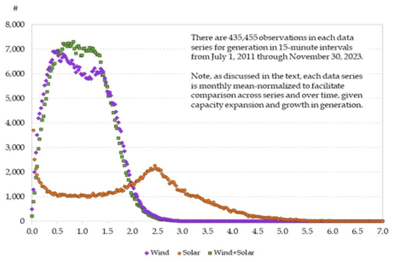
Mean-normalized distributions of wind, solar, and wind + solar.
Combined-cycle natural gas generation provides most flexible dispatchable capacity in ERCOT. Since 2010, new natural gas plants have merely compensated for older coal facility retirements. When wind plus solar output is high, dispatchable generators are either taken offline, reducing their total operating hours, or they face low, sometimes even negative, wholesale electricity prices. Intermittency also increases the ramping costs of thermal generators. Reduced profitability weakens incentives to maintain old or invest in new dispatchable thermal capacity.
As Figure 4 shows, the annual peak load has exceeded dispatchable thermal capacity since 2018. More ominously, Figure 6 shows that daily peak loads have been exceeding dispatchable thermal capacity with increasing frequency. Energy Emergency Alerts (EEAs) and Voluntary Conservation Notices (not pictured), issued when operating reserve margins pass specified thresholds according to rules established by the Public Utility Commission of Texas (PUCT), have also become increasingly frequent.
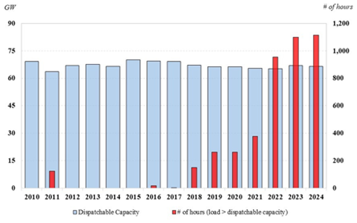
Hours when load exceeded dispatchable thermal capacity, 2010 to 2024.
Charged batteries are also dispatchable, but their ability to store energy is very limited compared to the fuels used by thermal generators. While batteries have proved valuable for providing ancillary services over very short periods, they have not yet been proven practical or competitive for providing bulk energy storage over longer periods.
Inadequate dispatchable capacity is likely to be a continuing problem. ERCOT’s Capacity, Demand, and Reserves Reports (https://www.ercot.com/gridinfo/resource) project that most new generation capacity will be wind and solar (very low current battery capacity makes its expected growth rate higher). Recent policies aimed at subsidizing additional dispatchable generation may be effective, but the large ERCOT electricity market is growing rapidly. Furthermore, over 36% of Texas’s operational thermal capacity is over forty years old (over 65% of coal capacity and 30% of natural gas capacity). Expected retirements and new capacity additions translate to a roughly 30 GW supply-demand gap to be filled by 2027, even excluding future load growth.
Another emerging problem is that much of the retiring dispatchable capacity, including over 6,500 MW of coal and natural gas retired between 2018 and 2022, is located near demand centers. The nine most populated counties in ERCOT, totaling 16.8 million, represent 56% of the state population (texas-demographics.com) and even more of the ERCOT load. Coal, natural gas, and nuclear account for roughly 90% of the installed capacity in these counties. The remaining 10% is mostly solar. Wind is sited in locations with better wind resources and lower land prices, which tend to be far from major demand centers. Transmission capacity is augmented slowly as long lines used at low capacity factors have high costs per unit of power transmitted. Transmission constraints can then prevent supply from meeting demand even if total system-wide generation is adequate. The substantial growth in wind capacity in recent years has thus presented ERCOT with a transmission challenge. A 2022 report (ERCOT December 2022b) found that both exports from renewable resource centers and imports into major demand centers faced transmission constraints. Another study (ERCOT January 2022a) identified a need for new transfer pathways and long-distance transfer technologies beyond the typical 345 kV circuit line to increase export capacity from remote generation sites.
4. Merit Order Effects
The merit order effect arises when increased renewables output generated at zero (or, with production subsidies, negative) marginal cost displaces higher marginal cost generation at the top of the merit order. Market-clearing wholesale prices set by the bid of the highest marginal cost generator ought then to decline.
The existence and magnitude of the merit order effect will vary not only from one system to the next but also over time within a given system. The set of generators actively supplying output can vary over time. Ramp-up and ramp-down costs cause the marginal cost for thermal generators to vary with output in previous periods and anticipated output in future periods. 7 Changes in the competitiveness of the wholesale market can affect the divergence between bids and marginal costs. Stronger connections with neighboring systems allow power imports or exports to dampen price movements. Finally, transmission constraints and the need to maintain power quality and system reliability may require generation units to be committed out of merit order.
An extensive literature has used wholesale electricity prices 8 from many locations to test for the merit order effect measured as a negative effect of increased renewables output on prices. Table A-1 in Tsai and Eryilmaz (2018) summarizes eleven such papers using data from Germany, Ireland, Italy, The Netherlands, and Spain, and four papers using data from different ISO’s in the U.S. Only two of the eleven use real-time market (RTM) as opposed to day-ahead market (DAM) data. Seven use data at the hourly frequency, three at the daily frequency, and only one uses data observed every fifteen minutes. All but two of them use data aggregated to the national or zonal level. Almost all of them estimate ordinary least squares (OLS) regression models. A paper that Tsai and Eryilmaz do not mention (Ketterer 2014), uses DAM price and predicted wind generation data from Germany to estimate a GARCH model. She finds that increased predicted wind generation reduces the mean but increases the variance of the day-ahead price. Cutler et al. (2011) use a non-parametric graphical presentation that illustrates a merit order effect on average but also substantial variation around that trend. They use thirty-minute RTM price, load, wind output, and net import/export data from South Australia at a time when wind output supplied about 16% to 18% of the load.
Of more relevance to our analysis, Millstein et al. (2021) examine hourly average LMP at the network connection points of approximately 2,100 wind and solar installations located across seven major electricity markets in the U.S., including ERCOT. They study a concept related to the merit order effect, namely variable renewable energy (VRE) value decline. This attempts to measure all factors affecting the change in revenues earned by wind and solar plants as the total capacities of such plants change. Reductions in average wholesale electricity prices via the merit order effect is partly responsible. Other critical factors include the correlations between outputs and wholesale prices. For example, wind output tends to be highest in early morning hours when low loads reduce wholesale prices, but in ERCOT, for example, the positive correlation between solar output and demand significantly increases value for solar plants. Millstein et al also identify reductions in LMP due to transmission congestion as a significant factor in VRE value decline. That finding illustrates the value of using LMP data instead of zonal average prices. Curtailments because of transmission constraints also marginally reduce the value of wind output in some ISOs including ERCOT. 9
Tsai and Eryilmaz (2018) is one of several papers that have focused on the merit order effect in ERCOT after LMP were introduced. 10 They use fifteen-minute SPP and output data for each thermal generator in ERCOT to examine how increasing wind generation affected thermal generator revenues. The main explanatory variable is fifteen-minute, ERCOT-wide, wind-generation output. Other variables included in the panel estimation were aggregate fifteen-minute ERCOT load, the natural gas price, 11 a vector of time dummies, and a node-specific fixed effect. They found a significant merit order effect, measured as a reduced price at non-wind resource nodes, that ranged from $1.45 to $4.45 $/MWh per additional 1 GW of wind generation, depending on the season and whether the fifteen-minute intervals were in peak or off-peak periods.
An earlier paper by Zarnikau et al. (2016) focused on the difference between the merit order effect of day-ahead wind generation forecasts on DAM prices versus the merit order effect of actual wind generation on RTM prices. They used ERCOT zonal hourly data to estimate two price regressions for each of the West, North, South, and Houston zones, yielding a system of eight seemingly unrelated linear regressions. The RTM results are most relevant to our analysis. A 1 GW increase in wind generation in the combined West and North zones reduced RTM from $2.43 to $6.27/MWh. A 1 GW increase in wind generation in the combined South and Houston zones had a larger range of effects (a reduction of $1.42 to $7.29/MWh for a 1 GW increase). However, since the same 1 GW increase is a smaller percentage increase in the combined West and North zones, the elasticities evaluated at the means range from −0.184 to −0.484 for the combined West and North zones versus from −0.033 to −0.176 for the combined South and Houston zones.
Rudolph et al. (2021) quantified the merit order effect of wind, solar, and nuclear generation on ERCOT zonal RTM prices at fifteen-minute intervals from 2015 to 2018. They used quantile regression (based on quantiles of the error as discussed in Section 7) and found that OLS misestimated the true marginal effects of the variables in all zones. They found variations of merit order effects by energy source, time of day, and zone. For increases in wind generation, the estimated elasticities ranged from −0.061 to −0.705 while for solar generation they were not statistically significantly different from zero (and ranged from −0.088 to +0.066).
Finally, Ajanaku and Collins (2024) compared merit order effects of wind generation on DAM and RTM prices in PJM and ERCOT. Like Rudolph et al. (2021) they used quantile regression analysis, but the data was more aggregated both temporally (hourly) and geographically (system-level). The explanatory variables in the RTM model were lagged RTM price, wind as a percentage of total load, load, separate positive and negative load forecast errors, the natural gas price, 12 cooling and heating degree days, and a set of time dummies. Since their data covers the period 01/01/2011 through 12/31/2019, which has witnessed dramatic changes in ERCOT demand and supply conditions (as detailed in Sections 2 and 3 above), it probably makes sense to scale the wind generation variable by dividing by total load. Nevertheless, the coefficient on the resulting “wind penetration” variable has a different interpretation to the estimates of the merit order effect obtained by the other papers mentioned above. 13 For the RTM in ERCOT, they found a small negative effect of wind penetration at the median and higher quantiles, but the effects were small and positive at the lowest quantiles.
Our analysis of the merit order effect in ERCOT LMP takes more care to avoid bias arising from correlations between the explanatory variables and the error terms, for example because of curtailment. First, we ensure that all explanatory variables are measured prior to when LMP are calculated. Since this may not be sufficient if the error terms are autocorrelated, however, we also use several instrumental variable methods.
More importantly, the higher temporal and geospatial granularity of our data allows us to separate a “true” merit order effect of increased VRE output, whereby it reduces the equilibrium price by displacing higher marginal cost thermal output, from its effects on transmission constraints. To explain this further, we need to understand how the LMP are calculated. The LMP (in $/MWh) at bus i in period t can be written:

ERCOT calls λt the “marginal energy price” or the “shadow price of power balance” and μit the “congestion component.” In practice, λt and the set of μit are calculated simultaneously by solving a linear optimization problem known as the security-constrained economic dispatch (SCED). Using the supply schedules submitted by generators, the SCED solves for the least-cost dispatch required to meet the prevailing loads while respecting various physical and operational constraints. The most important constraints for our purposes are limits on energy flows through transmission elements (such as lines, transformers, and switchyards) required to protect against thermal overload, transient instability, dynamic instability, or voltage collapse.
More explicitly, λ is the solution for the Lagrange multiplier on the system-wide power balance constraint. 14 Without any physical and operational constraints, the costs of dispatching generation to meet the load should be minimized, and λ should equal both the incremental cost of supplying a marginal additional load 15 and the bid to supply incremental power from the active generator with the highest bid. However, satisfying the constraints may require units to be committed out of merit order as determined by the submitted supply schedules. The SCED will also fail to minimize cost if price caps limit any of the calculated LMP. 16
Each transmission constraint j in the SCED solved at t has an accompanying Lagrange multiplier, νjt ≥ 0, that becomes positive if constraint j binds. Separately from the SCED, ERCOT determines a “shift factor”
Equations (1) and (2) imply that
Since the data allows us to separately identify λ and μ, we measure the merit order effect by the change in the shadow price of power balance λ as increased wind or solar generation displaces thermal generation. As observed when discussing Millstein et al. (2021), however, congestion effects are also relevant when assessing the value of adding wind or solar generation to different locations on the network. We therefore also separately examine how changes in generation affect the probability that at least one μit ≠ 0 and the cross-sectional distribution of μit when one or more μit ≠ 0.
5. Data
We obtained T = 44,649 successive observations (around 152 days of mostly 18 5-minute intervals) of LMP ($/MWh) for the approximately 19 16,500 electrical buses on the network from July 6 to December 5, 2023. We obtained data on λ ($/MWh) for the same periods. From (1), subtracting λt from LMP it yields μit ($/MWh) for bus i in period t.
Potential explanatory variables included load, generation from thermal (defined as generation from coal plus natural gas plus nuclear), wind, and (utility-scale) solar sources, and physical response capability (PRC) (all measured in GW). These were collected for each 5-minute interval in the 152-day sample period. The values reported at, for example, 1:05 pm are the averages over the interval 1:00 pm–1:05 pm. To reduce endogeneity bias, the values pertain to the five-minute interval closest to, but preceding, the LMP measurement time. 20
The pairwise correlations of load with thermal (.890) wind (.502), and solar (.293), of thermal with wind (−.079) and solar (−.380), and of wind with solar (−.383) are not large enough to raise concerns about multicollinearity. However, the correlation between load and the sum of thermal, wind, and solar is very high (.9995). The sum can exceed load (energy delivered) due to transmission losses, which vary with load and the distribution of loads and generation inputs across the network. Conversely, load can exceed the sum when other generation (hydroelectric, biomass, or distributed generators), supply from storage, 21 or imports of DC electricity from neighboring systems are high. In our sample, the sum deviates from load by 6.7% at most, and is within 2% of it for 95% of the periods. The VIF statistic in an OLS regression of λ on load, thermal, wind, and solar strongly implies multicollinearity is a problem. Hence, we excluded load from the explanatory variables in the subsequent analysis.
ERCOT defines PRC as “the generation and load resources that are available to respond quickly to system events in case of sudden changes, such as an unexpected outage at a large generating unit.” This measure of spare capacity changes over the day as generators or loads are turned on or off. Higher PRC could be related to transmission constraints for several reasons. Lower load would reduce transmission levels and could also raise PRC. Higher load forecasts also produce more available online capacity (and thus higher PRC), and the automatic deployment, or governor response, of PRC generators might unintentionally reduce transmission congestion by altering transmission patterns.
The scatter plots in Figure 7 reveal that wind tends to be lower when load is higher, while the opposite is true for solar. Whereas wind output is high in the early morning hours, solar output is high when demand for power for air conditioning is high. The stripes in the scatter plot of solar against load occur around sunrise and sunset. They reflect a strong correlation between ambient temperature and incident solar radiation. The positive correlation between load and thermal reflects the backup role of thermal plants. The decline in PRC with load suggests that plants that provide PRC when load is low are called upon for normal supply when load is high.
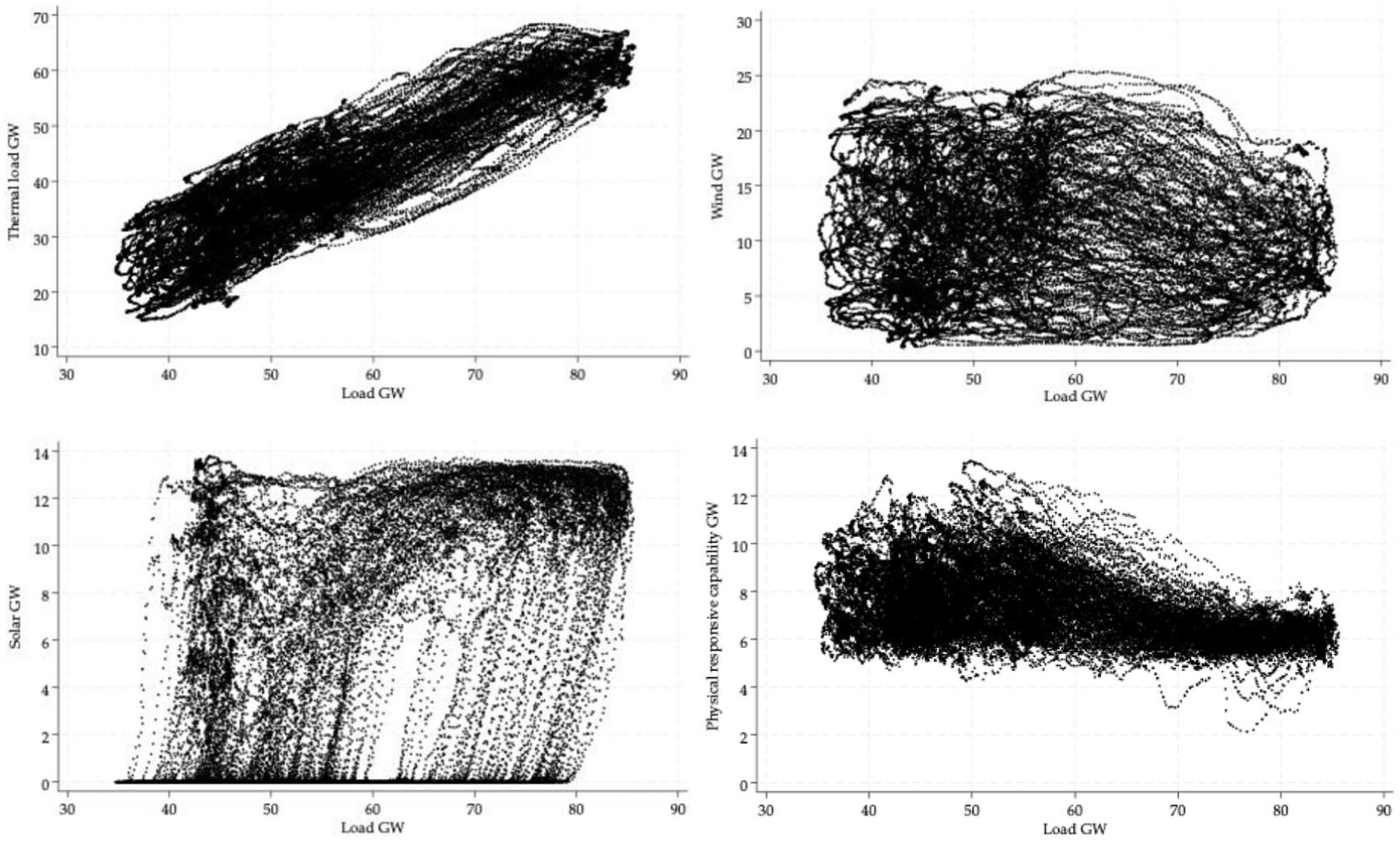
Scatter plots of generation and PRC against load.
We also obtained forecasts of the total ERCOT load and the loads in the four zones depicted in Figure 2. We converted the latter to load shares for the North, Houston, and South zones. The West zone share is dropped to avoid collinearity with the constant term. The forecasts, published at half past every hour, pertain to averages expected over an entire hour starting thirty or ninety minutes later. We use the most recent forecasts for each hour to derive forecasts for each five-minute interval. These are weighted averages of forecasts for the hour containing the five-minute interval with forecasts for the previous or following hours. We explain the weighting procedure with an example.
Consider a five-minute interval between 2:00 pm and 3:00 pm. In the first thirty minutes, we use a weighted average of the final forecast (made at 12:30 pm) for 1:00–2:00 pm and the final forecast (made at 1:30 pm) for 2:00–3:00 pm. Weights on the 2:00–3:00 pm hour forecast start at 0.5225 for the 2:00–2:05 pm interval and increase linearly to a maximum of 0.9725 for the 2:25 pm–2:30 pm interval. At the end of that interval, a final forecast for 3:00 pm–4:00 pm is published. The remaining five-minute intervals in the 2:00–3:00 pm hour use a weighted average of the newly published 3:00–4:00 pm forecast with the same 2:00–3:00 pm forecast. The weight on the 2:00–3:00 pm forecast remains at 0.9725 for the 2:30–2:35 pm interval. It then declines linearly across successive five-minute intervals, reaching 0.5225 for the 2:55–3:00 pm interval.
Since the correlation between the expected and measured loads is very high, an OLS regression of expected load on thermal, wind, and solar yields an R2 = .9960. Thus, we do not include expected load as a separate explanatory variable. However, the difference between load and expected load could measure stress on the system. As in Ajanaku and Collins (2024), to allow the effects of the actual exceeding the expected load to differ from the effects of the expected exceeding the actual, we defined two variables:

While various long-term pricing contracts 22 should reduce the dependence of load on calculated LMP, reverse causation could remain an issue. Large industrial customers might respond to real-time SPP. ERCOT customers with demand-side management contracts could have their supply curtailed at short notice, typically when operating reserve margins cross certain thresholds. These are likely to be times with high LMP. Wind and solar generation can be curtailed when the network becomes congested. PRC may also have an endogenous component if ERCOT schedules more responsive capability as the system load approaches capacity.
Measuring the explanatory variables prior to when the LMP are calculated should reduce endogeneity bias. However, it may not eliminate it because the error terms could be autocorrelated. Then, lagged explanatory variables could also be correlated with the current period error terms. We therefore added variables that can serve as instruments. They need to be correlated with the explanatory variables and affect the calculated LMP only via the included explanatory variables.
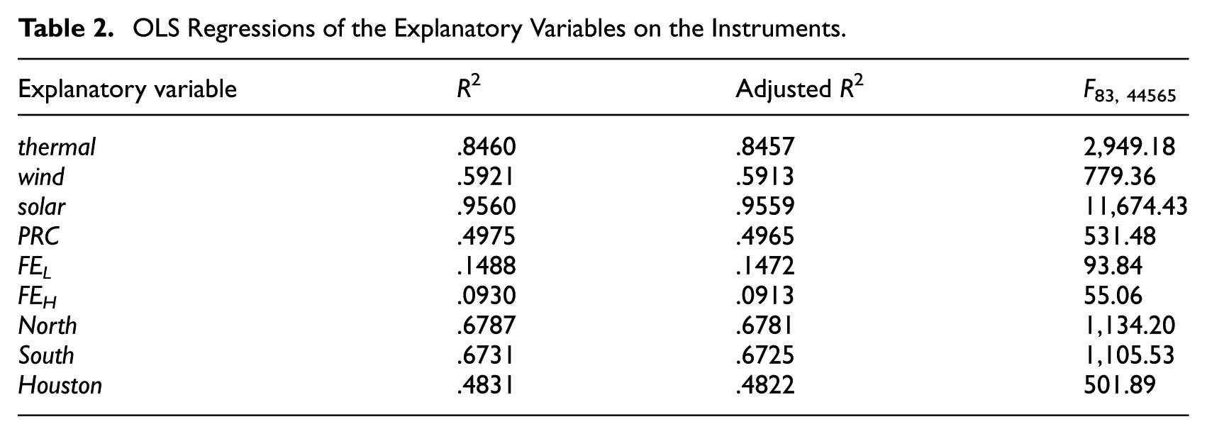
Since electricity demand is correlated with working hours, indicator variables for the day of the week and the hour of the day (measured allowing for daylight saving, not universal time) should qualify as instruments. After omitting one day and one hour, these provide twenty-nine instrumental variables (hereafter IV). We also used data from all nine U.S. Climate Reference Network (USCRN) stations across Texas. These stations continuously measure, among other variables, temperature, wind speed, solar radiation, relative humidity, and precipitation. 23 Wind speed and solar radiation should directly affect wind and solar generation. Both temperature and humidity, and their combined effect, should affect air conditioning demand. Precipitation will be correlated with cloud cover, which would affect solar generation and limit the use of air conditioning. The weather data is reported as five-minute averages with the same measurement intervals as the explanatory variables discussed above. The six weather variables measured at nine stations provide another fifty-four IV. The R2, adjusted R2, and F-test values in Table 2 show that these eighty-three variables have explanatory power for the explanatory variables in Table 3. The relationship is weakest for FEL and FEH, but even in those cases, forty or more of the coefficients on the IV are significantly different from zero at p-values less than .001.
OLS Regressions of the Explanatory Variables on the Instruments.
Moments of Explanatory Variables as a Function of χ.
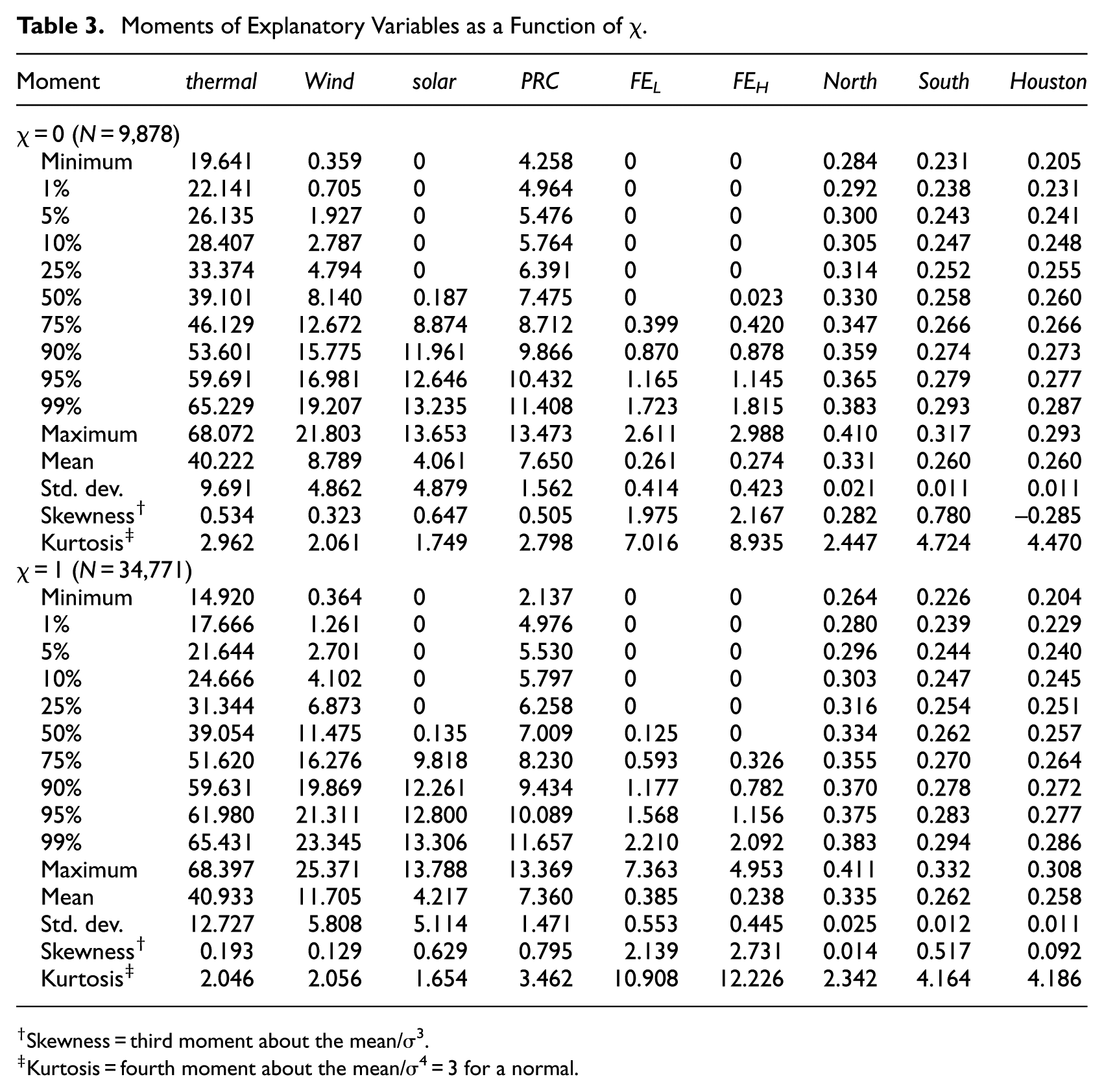
Skewness = third moment about the mean/σ3.
Kurtosis = fourth moment about the mean/σ4 = 3 for a normal.
6. What Makes Transmission Constraints Bind?
In about 22 percent of the five-minute intervals, the cross-sectional standard deviation σ in LMP is zero, implying binding transmission constraints were absent. To investigate the causes of binding transmission constraints, we defined an indicator variable, χ = 0 for σ = 0 and χ = 1 for σ > 0, and estimated a probit model with χ as the dependent variable.
Table 3 gives moments of the explanatory variables as a function of χ (in GW apart from the regional shares). The mean thermal is about 1.8% higher, and the mean solar is about 3.8% higher when χ = 1. The distributions of thermal and solar also are more dispersed when χ = 1. The quantiles below the median are lower, and those above it are higher. The standard deviations and the fourth moments around the mean are also higher.
The entire distribution of wind is shifted to the right when χ = 1. All quantiles are larger, although the extent of the increase is greater for the larger quantiles. The mean of wind is more than 33% larger when χ = 1. The standard deviation is also slightly larger, as are the third and fourth moments around the mean.
The distribution of PRC across the two subsets is more similar for high values than for low ones. While physically responsive generators can help mitigate the effects of binding transmission constraints, ERCOT does not procure ancillary services on a regional basis and PRC is not directly used to manage congestion. Thus, physical responsive generators are not always well-located to alleviate the constraints, and PRC can remain large in the presence of transmission constraints.
Forecast errors where load exceeds the expected load tend to be larger when χ = 1. The quantiles that are not zero are all larger, as is the mean. FEL also is more dispersed when χ = 1 with a higher standard deviation and kurtosis. It is also more positively skewed. Forecast errors where the expected load exceeds load can also be much larger when χ = 1. However, in this case, the median, 75th, and 90th quantiles are higher when χ = 0. The mean FEH is also higher when χ = 0. The distributions of forecast zonal load shares are more similar for the two values of χ.
Table 4 gives the parameter estimates for two probit models for χ. The first column presents maximum likelihood estimates, assuming that the explanatory variables are uncorrelated with the error. The heteroskedasticity- and autocorrelation-consistent (HAC) Huber-White sandwich standard errors are in parentheses beneath the coefficient estimates. The second column of Table 4 gives estimates for the probit model using IV and Newey’s (1987) minimum-chi-square two-step estimator. The standard errors are derived from asymptotic theory, but bootstrap standard errors are almost the same except for the coefficients of FEH and FEL, where p-values increase slightly to .001. The discussion focuses on the IV results since a Wald test (
Probit Models for χ as the Dependent Variable.
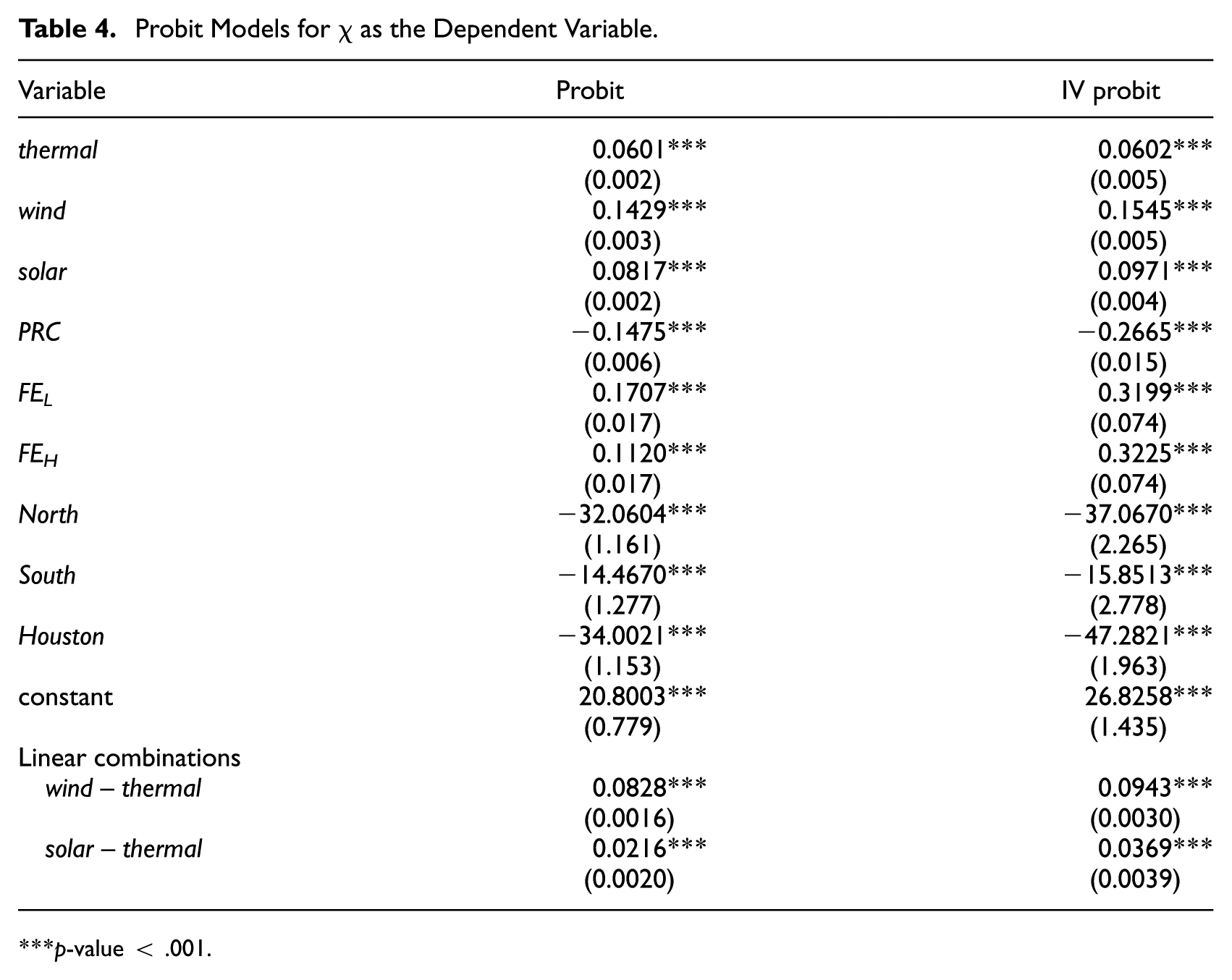
p-value < .001.
The coefficient on thermal measures the effect of increasing thermal output while holding the other explanatory variables, including especially wind and solar, constant. That means that load is increasing by approximately the same amount as thermal. The small, statistically significant positive value is consistent with the notion that increasing the amount of power transmitted across the network increases the probability that χ = 1. 25
Similarly, the coefficient on wind represents the effect of increasing wind and load by approximately the same amount. The larger value suggests that the extra wind generation usually is not well-located relative to the extra load, further increasing the probability that χ = 1. In fact, the coefficient of wind – thermal measures the effect of an increase in wind accommodated by an equal back-down in thermal. The strong positive coefficient supports the conclusion that the additional wind generation is less well placed to serve the load than was the displaced thermal generation.
Increasing the output from utility-scale solar generators in concert with an increase in load has a similar, albeit smaller effect than a matched increase in wind and load. An increase in solar accommodated by an equal reduction in thermal also increases the likelihood of binding transmission constraints, but by a lesser amount than for wind.
Higher PRC substantially reduces the likelihood of a binding transmission constraint. The positive coefficients on FEL and FEH imply that any load forecasting error increases the likelihood of binding transmission constraints. The coefficient on North measures the effect of increasing the forecast load share in the North zone holding South, and Houston fixed. It thus measures the effect of a forecast switch in load from the West to the North zone. This reduces the likelihood that χ = 1. Similarly, a forecast switch in load from the West to the South or Houston zones also reduces the likelihood that χ = 1. The difference North–South measures the effect of a switch in load from the South to the North zone, which also reduces the likelihood that χ = 1, as does a switch in load from the South to the Houston zone or the North to the Houston zone. Evidently, transmission capacity is most needed in the West, then South, then North zones.
7. Determinants of the Shadow Price of Power Balance λ
Table 5 gives summary statistics for the distributions of λ when χ = 0 versus when χ = 1. A Wilcoxon rank-sum test and a Kolmogorov–Smirnov test both reject the hypothesis that the two distributions are identical at a better than .0001 p-value.
Summary Statistics for the Distribution of λ as a Function of χ.
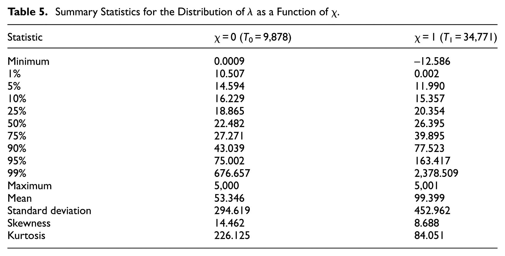
The distribution when χ = 1 has more low values, including some negative values. 26 Nevertheless, λ tends to be higher overall when χ = 1. Both the mean and the median are larger. The almost identical maximum values probably reflect the price ceilings (see footnote 15). The distribution of λ when χ = 1 is also more variable. The standard deviation σ and the third and fourth moments around the mean (skewness × σ3 and kurtosis × σ4) are much higher. The distribution when χ = 1 also has more values less than 16 or greater than 75.
Table 6 presents full sample (44,649 observations) OLS and generalized method of moments (GMM) IV estimates of the effects on λ of the same explanatory variables
27
as used in Table 4. The IV in the GMM estimation also are the same as were used in Table 4. The OLS standard errors are HAC Huber-White sandwich estimates, while the GMM standard errors are also HAC using a Newey-West kernel with the lag order selected using Newey and West’s (1994) optimal lag-selection algorithm. For the OLS, R2 = .0960, the RMSE = 402.69, and the test of joint statistical significance of the parameter estimates is
Regression Models for λ.
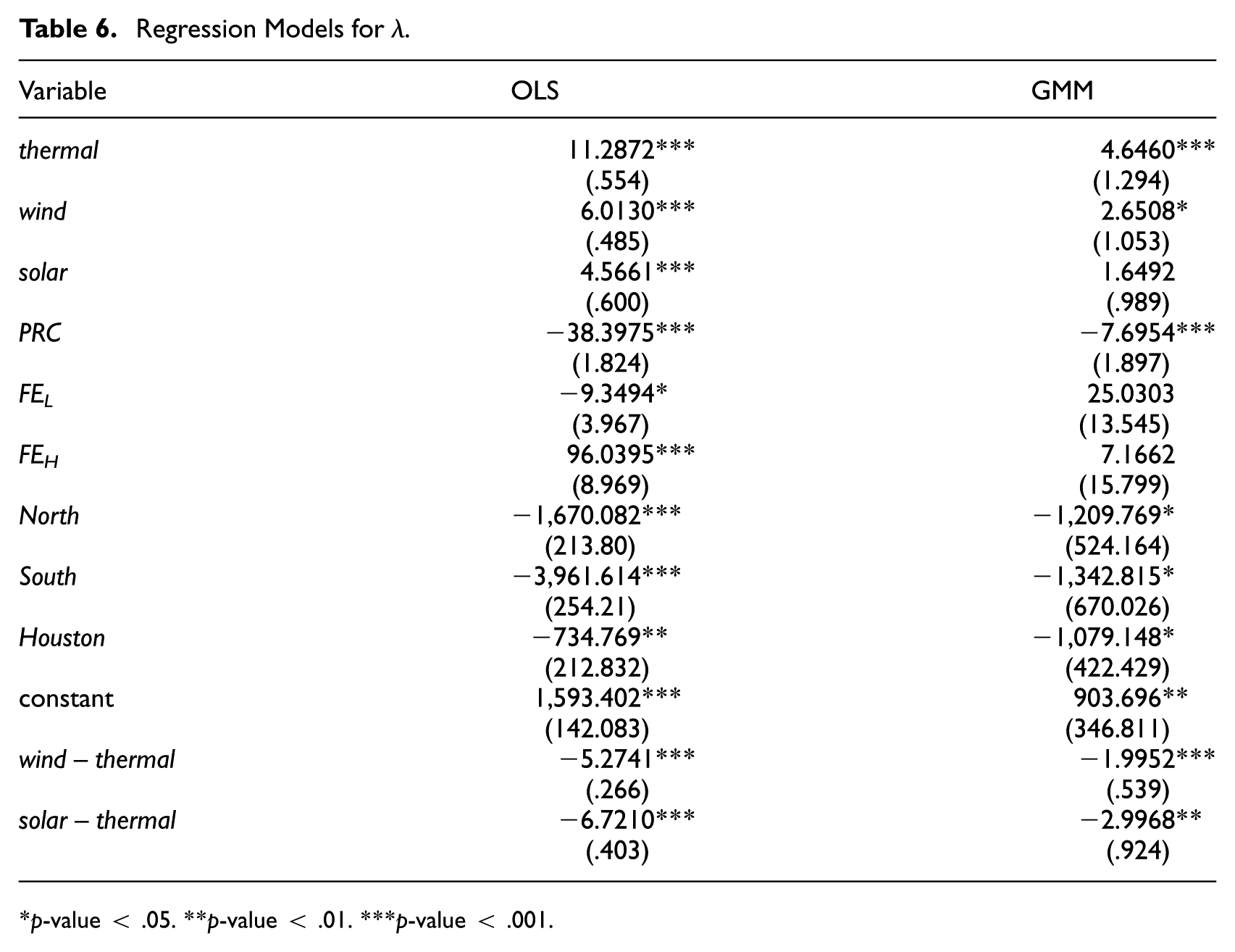
p-value < .05. **p-value < .01. ***p-value < .001.
The implications of the estimates for the merit order effect are of most interest. The negative coefficients on wind – thermal and solar – thermal imply that increasing wind or solar while backing out an equivalent amount of thermal generation reduces λ as hypothesized. A 1 GW swap of wind for thermal reduces λ about $2/MWh. A 1 GW solar/thermal swap reduces λ about $3/MWh. Although the difference between displacing thermal by wind versus solar is not statistically significantly different at the 10% level, the smaller magnitude of the coefficient on wind – thermal suggests that increased wind output may require more out-of-merit-order scheduling of thermal plants to maintain system stability. This is also the implication of the positive coefficient on wind alone, which implies that a 1 GW increase in wind matched by a 1 GW increase in load raises λ about $2.65/MWh. By contrast, the smaller coefficient on solar alone (which is not statistically significantly different from zero at the 5% level) suggests that a matched change in solar and load requires much less re-scheduling of thermal plants.
We can also compare our estimated merit order effects in ERCOT with those obtained by prior authors as discussed in Section 4. Since the growth of solar generation in ERCOT has been relatively recent (Figure 4), those papers focused on wind. Their estimates ranged from a decrease of $1.40/MWh to $7/MWh for a 1 GW increase in wind (holding load fixed). Our OLS estimates are toward the upper end of that range, while the IV estimates are closer to the lower end.
Turning to other variables, 1 GW of additional PRC is estimated, consistent with its purpose, to significantly reduce λ by around $7.70/MWh. The large change in the coefficient on PRC from the OLS to the GMM estimation suggests that the endogenous reaction of PRC to current conditions further moderates λ. Forecasting errors of either sign increase λ on average, but the effect of under-forecasting load is substantially larger. However, neither of the coefficients is statistically significant from zero at the 5% level (the coefficient of FEL has a p-value of .065). Finally, the estimated coefficients on the expected regional load shares imply that a higher fraction of load in the West zone tends to increase λ. Shifts in forecast load shares between the North, South and Houston zones have about one-quarter the effect. A shift from either North or Houston to South, or from Houston to North, decreases λ.
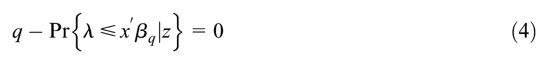
Following Rudolph et al. (2021) and Ajanaku and Collins (2024), quantile regression can deal with heteroskedasticity by allowing the relationship between the explanatory variables and λ to depend on the quantiles of the random error. Let xt denote the vector of explanatory variables at t including 1 as the first element. For quantile q, choosing parameter vector βq to ensure Pr{λt≤xt′βq} = q is equivalent to choosing βq to minimize

For q = 0.5 (the median), βq is the least absolute deviations estimator, which focuses on the “average” relationship, like least squares, but is less sensitive to outliers. However, for q = 0.05, for example, observations with negative errors receive 19 times the weight of those with positive errors. Conversely, for q = 0.95, observations with positive errors dominate the estimation. Quantile regression thus allows the relationship between λ and x to differ for extreme lower outliers, “more typical” observations and upper outliers. Heteroskedasticity in the error term related to x will be reflected in different values of βq for different values of q.
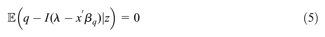
The analysis conducted thus far suggests that the explanatory variables are likely to be correlated with the error term. Fortunately, the analysis also suggests that the proposed IV are valid instruments. Suppressing t subscripts and denoting the vector of IV by z, we can estimate the IV quantile regression model by choosing βq for quantile q to satisfy
Using the definition of expectation (4) can be written
where I(u) = 1 for u ≤ 0 and 0 otherwise. Let
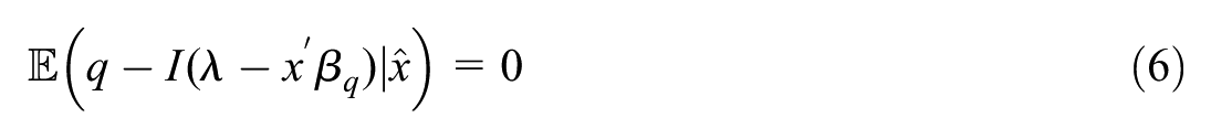
The moment condition (6) can form the basis for GMM estimation, but the function I(u) is not smooth. The estimator proposed by Kaplan and Sun (2017) replaces I(u) with a smooth approximating function.
Table 7 reports the IV quantile regression estimates (using the same IV as above). 28 Many coefficients in Table 7 are statistically significantly different from zero. 29 The joint test that they are all zero is soundly rejected. The hypothesis that the coefficients are identical across values of q is also strongly rejected. The test comparing the coefficients to those estimated by quantile regression based on (3) soundly rejects the hypothesis that the explanatory variables are exogenous.
Instrumental Variables Quantile Regression Estimates for λ (T = 44,649).
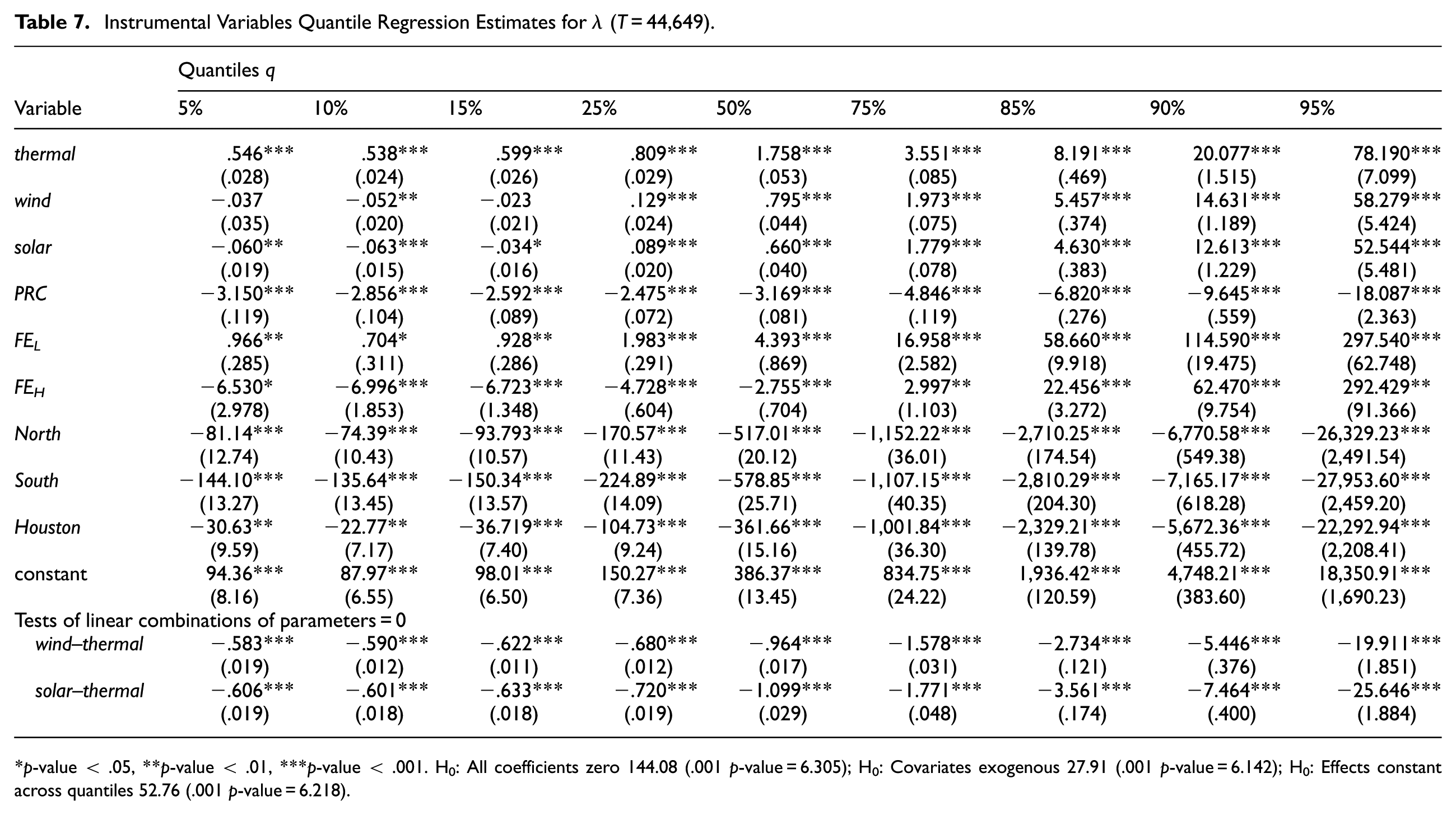
p-value < .05, **p-value < .01, ***p-value < .001. H0: All coefficients zero 144.08 (.001 p-value = 6.305); H0: Covariates exogenous 27.91 (.001 p-value = 6.142); H0: Effects constant across quantiles 52.76 (.001 p-value = 6.218).
The coefficients on thermal, wind, and solar reflect situations where other generation outputs are fixed while increases in one of thermal, wind, or solar approximately match increased load. The positive, and for q ≥ 0.1 increasing, coefficients on thermal suggest that the aggregate supply curve for the thermal power plants is convex. The negative coefficients on wind and solar for q = 0.05, 0.1, and 0.15 suggest that when
The negative coefficients in the last two rows of Table 7 reveal a merit order effect at all q for both wind and solar. Consistent with the IV GMM results, the effect is larger for solar, although barely so for the 10th and 15th quantiles. While the magnitudes of the wind – thermal coefficients increase monotonically with q, the magnitudes of the solar – thermal coefficients slightly decrease from q = 0.05 to q = 0.10 but then increase to end up approximately one-third larger than the coefficient on wind – thermal for q ≥ 0.85. For the most extreme 5 percent positive outliers, a 1 GW wind/thermal swap reduces λ about $20/MWh, while a 1 GW solar/thermal swap reduces λ about $25/MWh. This is consistent with the notion that the marginal costs of the marginal thermal generator are higher under extreme conditions. These effects are larger, and more sensitive to q, than estimated in Rudolph et al. (2021) or Ajanaku and Collins (2024). However, they estimate effects on RTM price (not just λ) after a change in wind or solar.
The coefficients on PRC measure the effect on λ of a 1 GW change in PRC holding thermal, wind, and solar constant, and hence load approximately constant. They imply that PRC becomes less critical for moderating movements in λ as q increases up to the 25th quantile but then becomes very important for large positive values of
Under-forecasting the load (FEL > 0) has a statistically significant positive and increasingly large effect on λ as q increases. Evidently, it leads to scheduled patterns of generation that are not least cost for the load. The negative coefficients on FEH for q ≤ 0.5 imply that over-forecasting load tends to reduce λ for lower values of
The coefficients on the forecasted load shares in the North, South, and Houston zones are all negative at all values of q. The magnitudes of the share coefficients decrease slightly as q increases from 0.05 to 0.1 but then increase substantially thereafter. As implied by the regression results in Table 6, a shift of load from the West zone to any of the North, South, and Houston zones raises λ. A shift from either North or Houston to South, or from Houston to North, decreases λ.
8. The Locations of Binding Transmission Constraints
We considered using a panel data estimator to examine influences on the distributions of the up to 17,000 μit in the T1 = 34,771 periods t where σ > 0. However, the number of nonzero μit can vary greatly across periods, with many μit truncated to zero in many periods. Also, since the number of buses on the network changes over time, the panel is unbalanced. The presence of endogenous regressors adds complications, as does the extremely large number of observations.
30
Instead we examine first the time averages of μit denoted
There is a trade-off between the number of buses present for all periods and the length of time we examine. We found 16,431 buses present for all 27,768 periods when daylight savings time was in place and at least one transmission constraint was binding. Table 8 gives summary statistics for the 16,431 time averages across the 27,768 periods.
Summary Statistics for Time Averages
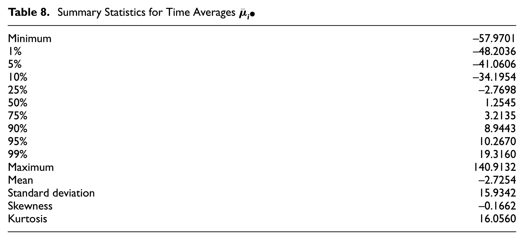
Following the discussion in Section 4, if μit > 0 an increase in demand at i in period t exacerbates constraints while if μit < 0 an increase in supply at i in period t exacerbates constraints. Hence, we call a bus with
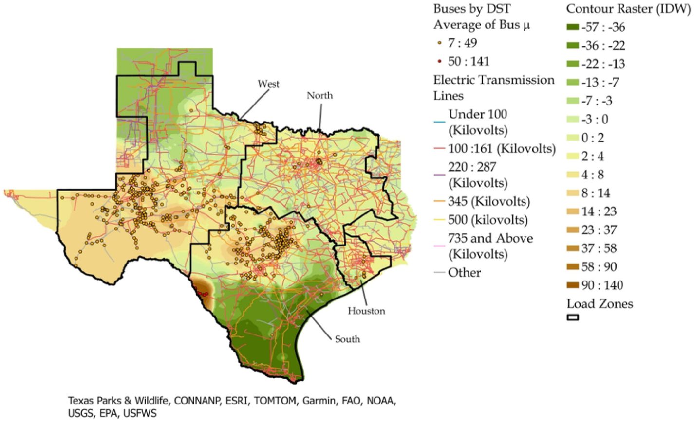
ERCOT does not publicly disclose bus locations. However, we were able to match 11,047 of the 16,431 buses to entries in the Velocity Suite data, which includes latitude and longitude coordinates. Figure 8 maps these 11,047 matched buses by their
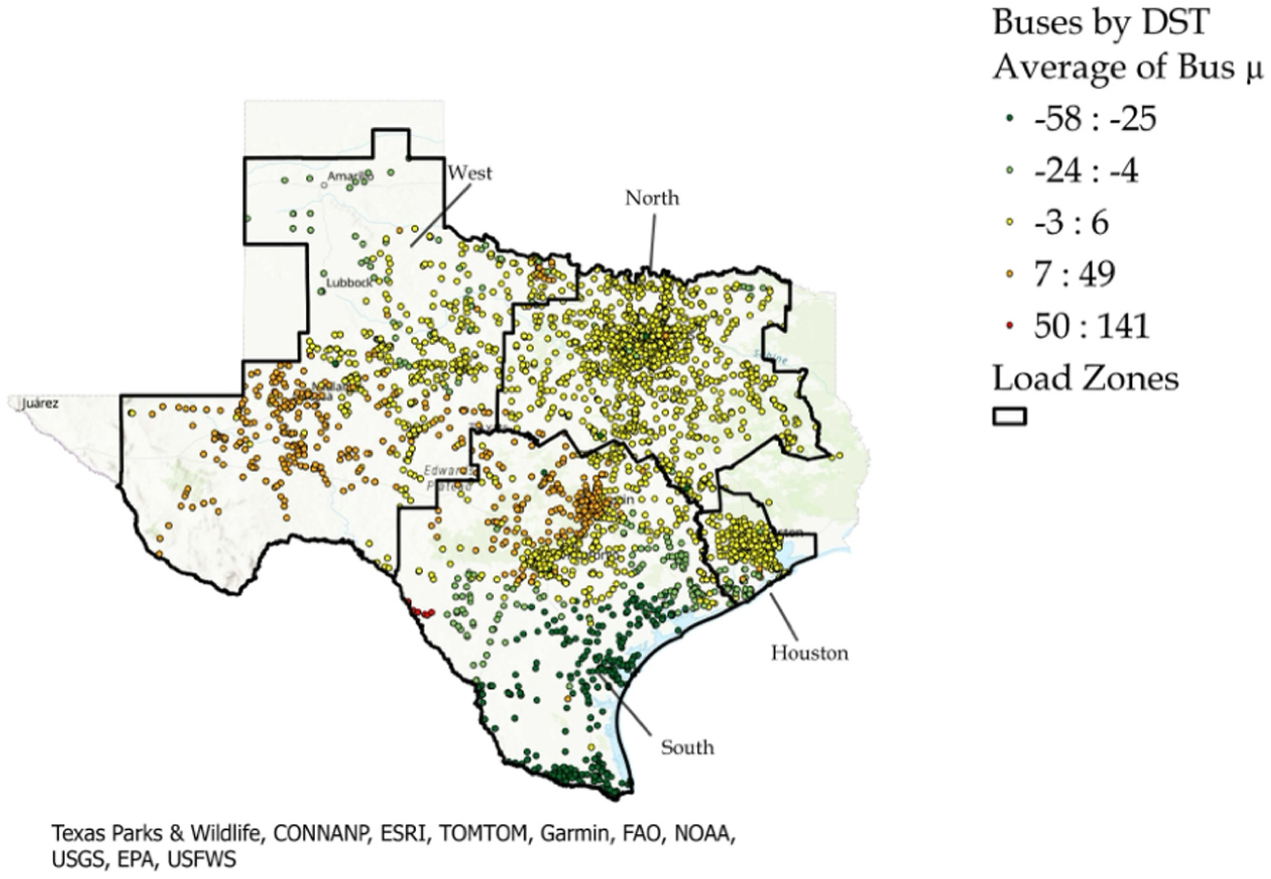
Bus locations colored by time averages
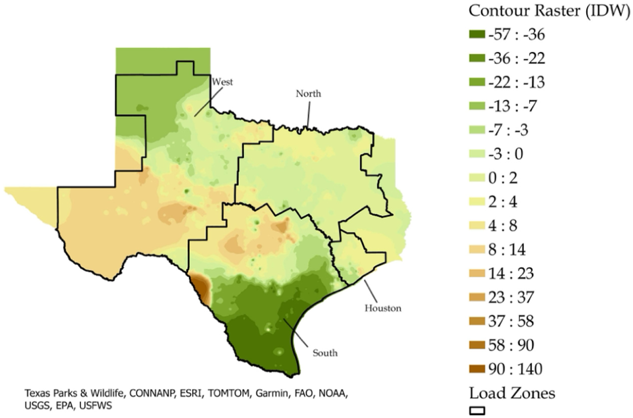
Contour map based on time averages
Figure 10 plots the 2,254 buses in the 2 most negative categories in Figure 8 against the colored contours from Figure 9. These more frequently and/or more severely constrained supply buses tend to be concentrated in the south and northwest, which Figure 11 shows are areas with substantial wind generation. Wind has expanded rapidly in South Texas in recent years without a corresponding build-out in new transmission capacity. Figure 11 also shows that thermal plants and near-zero values of

Locations of the most predominant constrained supply buses.
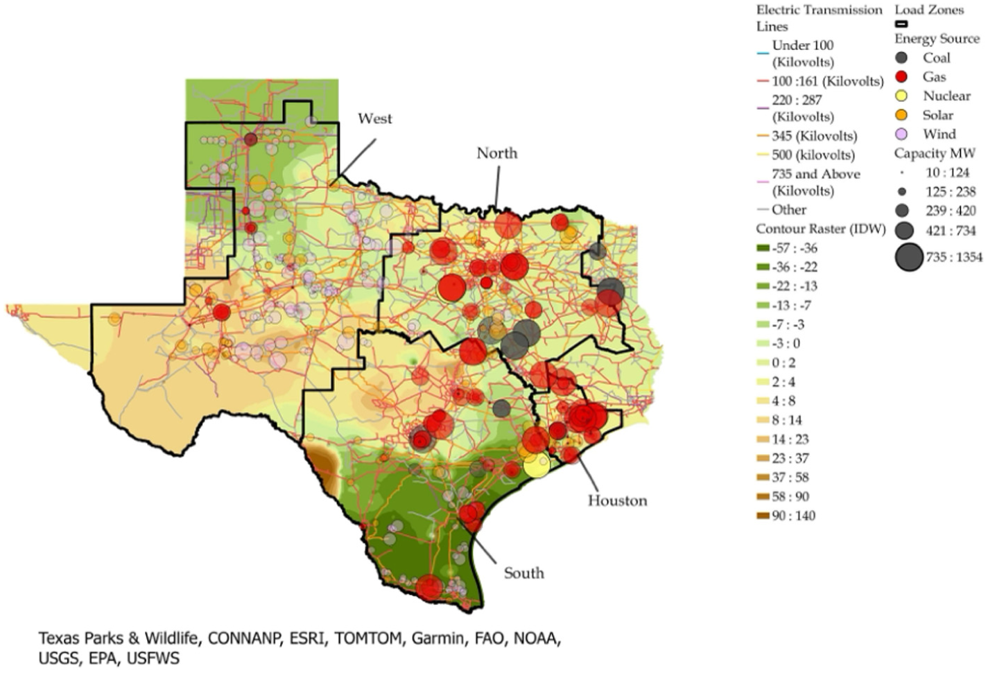
Locations of major generators in Texas.
Figure 12 plots the 1,571 buses in the 2 most positive categories in Figure 8. These more frequently and/or more severely constrained demand buses are around Laredo and Eagle Pass in the Mexican border area, followed by the Austin area in Central Texas, and then the oil-producing regions in the Permian Basin. As noted in Section 2, Central and West Texas have been areas of recent rapid load growth. These constrained demand buses also generally coincide with projects selected for evaluation in the Regional Transmission Plan (ERCOT 2024b). In that report, ERCOT highlighted locations of new loads as a critical driver of flow patterns.
Locations of the most predominant constrained demand buses.
ERCOT (2024a) highlighted the top 10 constraints as of November 2024 with projections to 2029. They coincided with the locations of constrained buses in the Permian Basin and the wind-producing regions in South and West Texas. The report identified the West Texas Export Interface as the second largest constraint with a congestion rent of $148M. Areas of severe constraints were projected to shift to the Northwest, south of Dallas, and areas near load centers. ERCOT’s top 10 planned improvements are located close to the Permian Basin, Dallas, and the Austin-San Antonio area.
Transmission constraints also can be addressed by adding dispatchable generation closer to demand centers. ERCOT’s latest estimate of capital costs for new units found that the overnight cost for all natural gas technologies is lower than any other technologies except for two-hour battery storage (ERCOT 2023). To send efficient siting signals to market participants or appropriately alert ERCOT about needed transmission upgrades, prices should reflect not only capacity constraints but also marginal transmission losses. Alleviating constraints via transmission upgrades could be less effective when the costs are “socialized” via a retail surcharge, as was done with the CREZ lines, since it weakens incentives to efficiently site new generation capacity or large loads. Including marginal transmission losses into LMP also would incentivize more efficient use of generation and improve short-run operations. 32
9. Influences on the Cross-sectional Distributions of μit
We examine next the cross-sectional distributions of the μit across all 34,771 periods when σ > 0. The rows in Table 9 present summary statistics for the cross-sectional quantiles and means (denoted
Summary Statistics of Cross-sectional
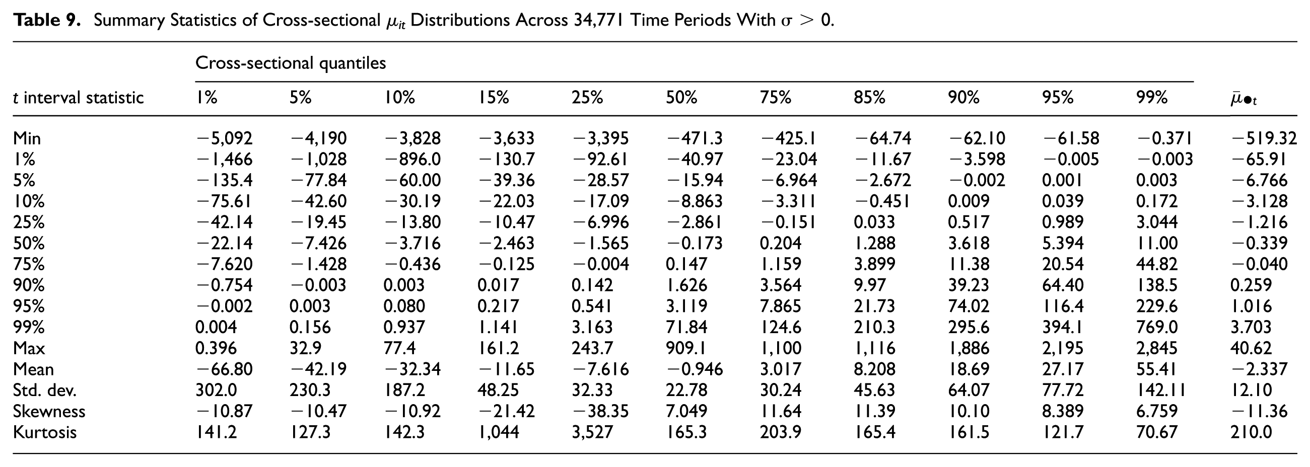
The means and medians cluster near zero. From Table 9, almost 80% of the medians and 93% of the means are less than 5 in magnitude. This reflects a tendency for a positive μit to cancel a negative μjt because a constrained line flowing power from bus i to bus j in period t contributes to both a negative μit and a positive μjt that depend on the same Lagrange multiplier. However, cancellation is incomplete for several reasons. First, the shift factor for bus i need not have the same magnitude as the shift factor for bus j. Second, since a line flowing power from bus i to bus j that is constrained in period t will generally contribute to μkt ≠ 0 for k ≠ i or j, equation (2) shows that each μit is affected by multiple constraints. Third, the number of buses negatively affected by a single constrained line need not equal the number of positively affected buses.
Figure 13 graphs the means (excluding the outlier −519.32 for clarity) against the medians and load. While the medians are relatively symmetrically distributed about zero, the means
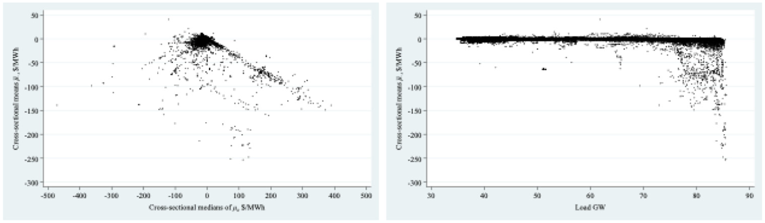
Scatter plots of
From the second graph in Figure 13, the most negative
More generally, the second graph in Figure 13 suggests that differences in load systematically affect the cross-sectional μit distributions. Table 10 gives the means of the cross-sectional moments in the column headings of Table 9 (and row headings in Table 10) for six arbitrarily chosen 10 GW categories of load. The number of five-minute intervals in each category is given by N. The means of the moments in columns 2 to 4 of Table 10 are alike but differ noticeably from those in the first column and substantially from those in column 6. Tentatively, we conclude that the cross-sectional quantiles tend to fall into three different load regimes with boundaries around 40 GW and 70 GW.
Means of Cross-sectional Moments of
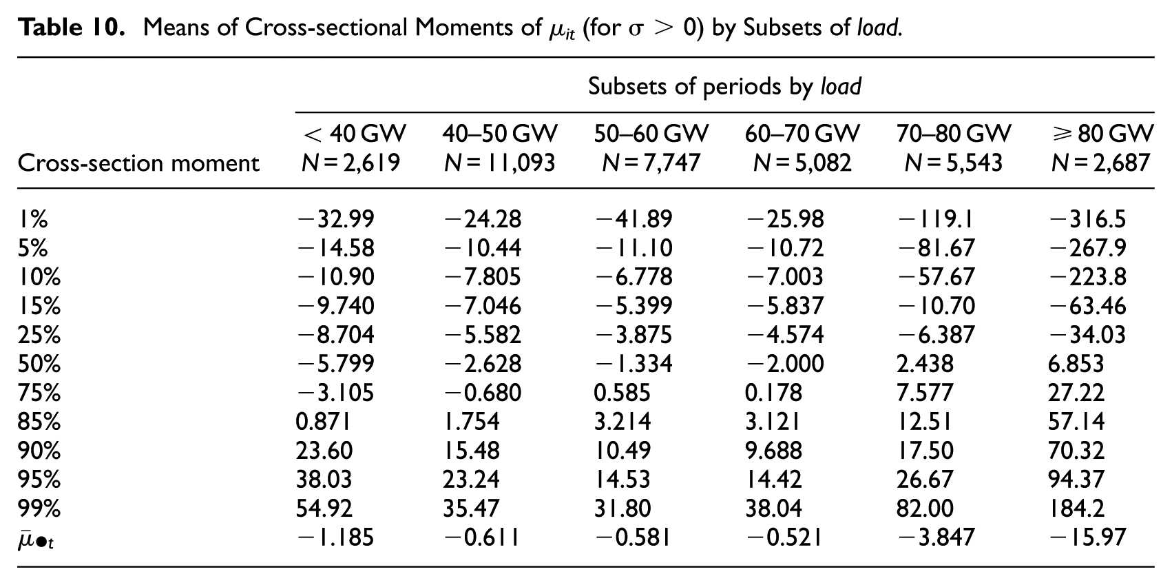
Figure 14 graphs Lowess smoothing regressions of the 5th, 10th, 25th, 50th, 75th, 90th, and 95th quantiles of the μit distributions against load. 33 The vertical lines at 44 GW and 72 GW separate the distributions into three different load regimes. The existence of three load regimes is consistent with the traditional approach in the economic analysis of electricity supply that distinguishes system behavior under base, intermediate, and peak load conditions.
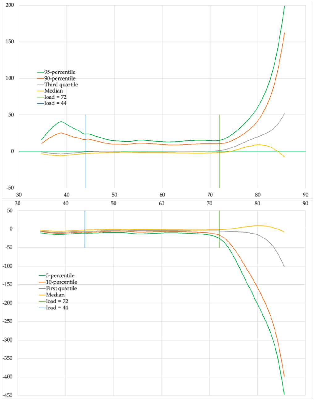
Lowess relationship between quantiles of the
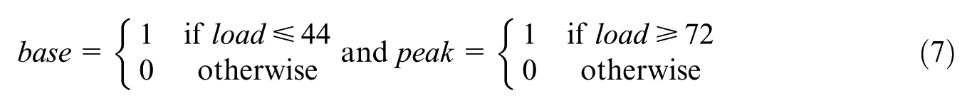
Based on this evidence, we estimated an IV GMM regression for each of the twelve cross-sectional moments while allowing parameters to vary under base, intermediate, and peak load conditions. This can be accomplished while preserving the time series ordering of the data by defining two indicator variables
and including the products of base and peak with the explanatory variables and the constant term. The coefficients on a variable x measure the effects during intermediate load periods. The effects of variable x in base or peak periods are obtained by adding the coefficients of x and x × base, or x and x × peak respectively. Each regression equation contains 29 explanatory variables, yielding 348 estimated coefficients. For clarity, Table 11 presents the results after eliminating any variable whose coefficient was not significantly different from zero at the 10% level both in the full model and when added back to the model in Table 11. The chi-square statistic in the fourth last row, which tests for the hypothesis that all the coefficients of variables excluded from an equation together equal zero, is far from being rejected in every case. The hypothesis that the coefficients of all the included variables are zero, tested by the statistics in the third last row of Table 11, is rejected at a p-value less than .001 in every case. The second last row gives Hansen’s J-test statistics for the validity of the overidentifying restrictions. None are statistically significant at the 5% level. The statistics in the final row are for the GMM C (or difference-in-Sargan) tests of the exogeneity of the explanatory variables. Apart from
GMM Regression Results for Quantiles and Means of the Cross-sectional Distributions of
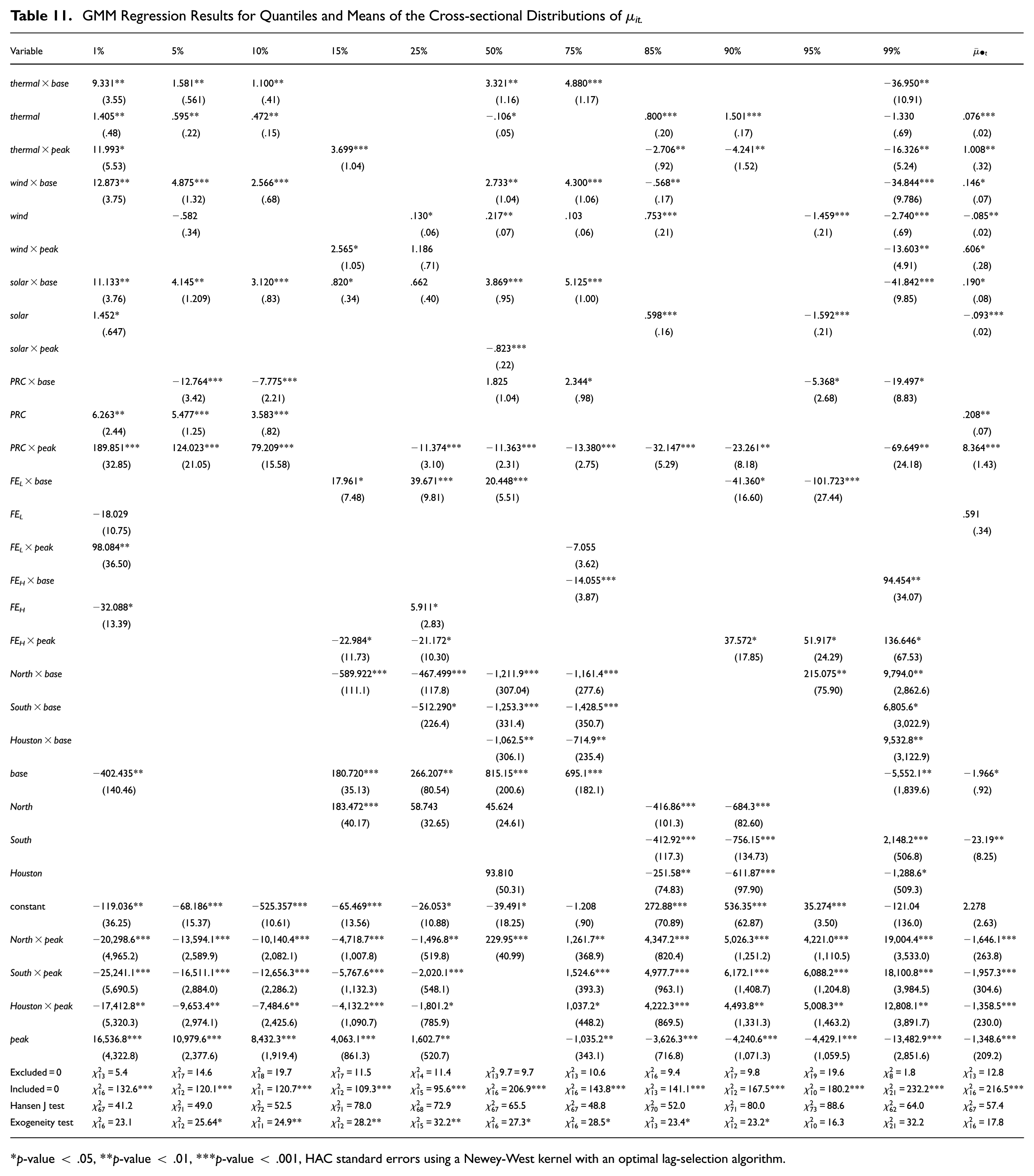
p-value < .05, **p-value < .01, ***p-value < .001, HAC standard errors using a Newey-West kernel with an optimal lag-selection algorithm.
The coefficients on wind or solar in Table 11 measure their effects on the prevalence or severity of transmission constraints. Prior studies that have used zonal and/or time averages of LMP or SPP would have recorded these as components of merit order effects.
To understand the consequences of a substitution of thermal generation by an equal amount of either wind or solar generation, we focus on the effects on the μit distribution of differences wind – thermal and solar – thermal. The differences in these coefficients measure effects under intermediate loads. To obtain the effects under base or peak loads, we need to consider the differences multiplied by base or peak respectively.
The left column of three graphs in Figure 15 plots the responses of quantile q (on the x-axis) of the μit distribution to changes in generation and load in the three regimes. The difference in vertical scales in the graphs (chosen to maximize the differences between the curves within each figure) shows that the effects are smallest under intermediate loads and largest under peak loads. As was evident also in Table 10 and Figure 14, this suggests that the system tends to be most stressed under peak loads and least stressed under intermediate loads.
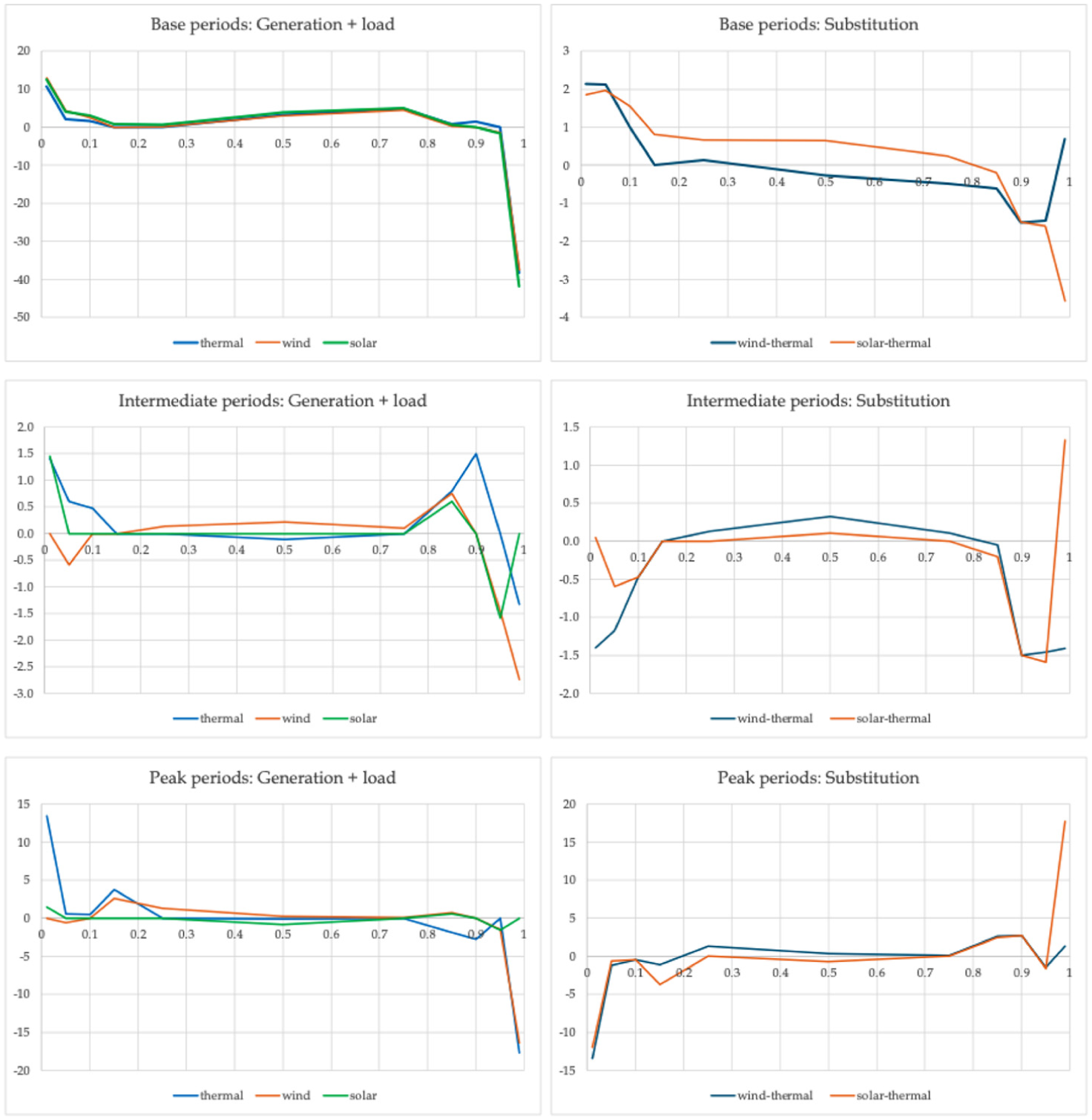
Generation effects ($/MWh) by quantile in the results from Table 11.
Similarly, the graphs in the left column suggest that the responses appear most uniform during base load periods. However, the right column of three graphs in Figure 15 show that this also is largely a consequence of the different vertical scales. The differences in coefficients are smallest in intermediate load periods.
To aid in interpreting the graphs in Figure 15, observe that the first column of Table 10 shows that, under base load conditions, the means of the quantiles are negative up to q = 0.75, slightly positive for q = 0.85, and then increase quickly with q thereafter. From the top left graph in Figure 15, increasing each type of generation commensurately with load tends to drive both negative and positive μ closer to zero and thus alleviate transmission constraints. Since this is so regardless of the type of generation, the increase in load appears to be the dominant factor.
The coefficients in the final column of Table 11 show that, in base periods, a 1 GW increase in both generation and load has approximately the same effect on
The top right graph in Figure 15 shows the effects during base periods of increasing either wind or solar by 1 GW while simultaneously backing out 1 GW of thermal. In the case of wind, the positive effects for q = 0.01, 0.05, and 0.1 and the negative effects for q = 0.85, 0.9, and 0.95 imply a reduction in the severity of constraints. Conversely, the positive effects for q = 0.99 and negative effects for q = 0.5 and 0.75 suggest that such a substitution exacerbates some transmission constraints. Increasing solar during base periods
35
by 1 GW while backing out 1 GW of thermal has positive effects on all quantiles up to q = 0.75, and negative effects for q = 0.9, 0.95, and 0.99, suggesting it tends to alleviate constraints. Nevertheless, the changes in
The middle two graphs in Figure 15 pertain to intermediate periods. As reflected in columns 2 to 4 of Table 10, the means of the quantiles in intermediate periods are negative up to q = 0.5, slightly positive for q = 0.75, and then increase with q, but not as much as in base load periods. The graphs in Figure 14 also show that the μit quantiles in base and intermediate periods differ mainly for the largest q. Increasing thermal along with load in intermediate load periods increases the 1st through 10th quantiles. These changes thus tend to reduce the severity of transmission constraints. On the other hand, the increases in the 85th and 90th quantiles suggest a tendency to exacerbate some constraints.
The middle graph in the right column of graphs in Figure 15 indicates that backing out 1 GW of thermal to accommodate a 1 GW increase in wind decreases the 1st through 10th (de-stabilizing) and 85th through 99th quantiles (stabilizing), while increasing the 25th through 75th quantiles (largely stabilizing).
The bottom two graphs in Figure 15 pertain to peak load periods. As reflected in columns 5 to 6 of Table 10 and the graphs in Figure 14, the μ distributions have much higher spreads in peak load periods. The graphs in Figure 15 indicate that changes in generation have much larger effects in peak periods. Increasing thermal along with load increases the 1st through 15th quantiles and decreases the 50th, 85th, 90th and 99th quantiles.
Increasing either wind or solar while backing out thermal exacerbates the effects of constraints on buses with the most extreme negative μit. Increasing solar while decreasing thermal also exacerbates constraints for buses with the most positive μit. Following the 1 GW wind/thermal swap,
Summarizing, the effects of 1 GW wind/thermal and solar/thermal swaps on the cross-sectional means
Since the merit order effects are our focus, we summarize the remaining results in Table 11 without graphing them. The effects of PRC under base loads are negative on the 5th and 10th quantiles, small and positive on the 50th and 75th quantiles, and negative again on the 95th and 99th quantiles. Under intermediate loads, greater PRC has a positive effect on the lowest three quantiles, but an effect that is indistinguishable from zero on the remaining quantiles. Higher PRC during peak loads has very strongly positive effects on the lowest three quantiles and negative effects on quantiles from the 25th and above. Apart from the negative effects of PRC on the 5th and 10th quantiles during base periods, these effects imply that increased PRC alleviates transmission constraints. The final column of Table 11 shows that increased PRC has moderate positive effects on
Under-forecasting (FEL > 0) base and intermediate loads exacerbates constraints on the buses with the most negative μit, but under-forecasting peak loads strongly alleviates them. Under-forecasting base loads also moderates the negative 15th to 50th quantiles and the positive 90th and 95th quantiles. The effects of FEL on
Over-forecasting load (FEH > 0) exacerbates constraints on buses with the most negative μit in all periods. Over-forecasting peak loads also exacerbates a wider range of constraints, as indicated in the reductions in the 25th and 50th quantiles and the large increases in the 90th, 95th, and 99th quantiles. Over-forecasting base loads also strongly increases the 99th quantile, indicating increased congestion of buses with the largest μit. On the other hand, the positive coefficient on FEH in the 25th quantile, and the negative coefficient on FEH × base in the 75th quantile, suggest that over-forecasting low-moderate loads can alleviate some moderate transmission constraints. The effects on
The effects of changes in forecast zonal load shares are in the second half of Table 11. Under intermediate loads, forecasting changes in zonal load shares have relatively minor effects. The largest is a forecast shift in load from the West to the South zone, which significantly increases the largest
Changes in forecast zonal load shares have larger effects on a wider range of quantiles in base periods. The 99th quantile is again most affected. A forecast shift of load from West to any other zone significantly increases the largest
Under peak loads, forecasting a lower West zone load share tends to greatly increase the dispersion in μit independent of where the offsetting share increase occurs. Large decreases in the 1st to 25th quantiles accompanied by somewhat smaller increases in the 75th to 99th quantiles suggest an exacerbation of transmission constraints. The accompanying decrease
10. Concluding Comments
ERCOT load has grown substantially over the last twenty years, driven by strong population and economic growth and electrification of activities including oil and gas operations. Because of the last factor, the West experienced the largest percentage increase. At the same time, wind and solar generation have supplied most of the increase in generation capacity. Total dispatchable capacity has changed little as net new natural gas capacity has barely matched coal retirements.
Texas wind generators tend to produce more output at night, while solar plants produce more in the early afternoon. This complementarity should enable more consistent output from the two sources together, but this effect is quite weak in practice. The standard deviation of the mean-normalized wind plus solar distribution (0.51) is only marginally smaller than the standard deviation of the mean-normalized wind distribution alone (0.55). Wind and solar often fail to produce when load is high and cannot be called upon at short notice to provide additional supply. The number of hours each year when load exceeds dispatchable capacity has increased substantially.
The added renewable capacity also is often located in sparsely populated areas remote from the major load centers. It requires substantial new transmission capacity extending over long distances and used at low capacity factors. Despite considerable expenditure on the CREZ lines built to bring remote wind-generated power to market, transmission capacity has again become inadequate.
The merit order effect is a frequently touted offsetting benefit of increased wind and solar generation. Since these sources have zero marginal costs, they shift the supply stack to the right. An increase in wind or solar generation as load remains unchanged reduces thermal (nuclear, coal, or natural gas) output. The marginal cost of the marginal thermal plant supplying output should decline.
To investigate how these developments have affected market prices, we examined bus-level LMP and generation output data covering around 152 days in the summer and fall of 2023. In contrast to the papers cited above, we used instrumental variable methods to avoid biased estimates arising from correlation between the explanatory variables and the error terms. The high temporal and geospatial granularities of our data allow us to separately examine the component of LMP arising from transmission constraints and identify a “true” merit order effect as a reduction in the shadow price of power balance λ when wind or solar output displaces thermal generation.
We found the merit order effect to be stronger for solar than for wind. In the IV GMM model, a 1 GW swap of wind for thermal reduced λ by about $2/MWh while a 1 GW solar/thermal swap reduced λ by about $3/MWh. In the IV quantile regression model, the reductions ranged from just under 60¢/MWh up to almost $20/MWh for a 1 GW wind/thermal swap, while for a 1 GW solar/thermal swap, the range was from almost 61¢/MWh up to almost $26/MWh. While statistically significantly different from zero, these effects are small in percentage terms. Higher levels of utility-scale solar and especially wind generation increase the likelihood of transmission constraints, which requires ERCOT to make out-of-merit order decisions to keep the system running.
Previous papers using wholesale prices to measure the merit order effect of wind and solar confound it with the effects of changes in the prevalence or severity of transmission constraints measured by the congestion components μ in LMP. A constrained transmission line flowing power between buses i and j in period t contributes to μit < 0 and μjt > 0. The magnitudes of the effects depend on shift factors, which essentially measure the distance of the bus from binding constraints and network density surrounding a binding constraint. A denser set of connections will give many alternative pathways for exchanging power with the rest of the network, thereby moderating the effect of a constraint.
In most periods t, the average μ across all buses,
The temporal averages of μit at each bus i,
Several results indicate that transmission constraints more severely affect generators than loads. Although the maximum
Transmission constraints are most frequent and severe under peak loads, but they are also more prevalent under base than intermediate loads. Both negative and positive μit tend to be larger in magnitude under base than intermediate loads, making the standard deviation and range noticeably larger. Apparently, the geographic distribution of loads and generation is often poorly matched under low load conditions. This is especially so when low loads are combined with high output from wind generators. As the EIA has noted, substantial curtailment of wind generation is occurring in ERCOT.
While the effects of changes in generation and load are of interest because of their implications for merit order effects, physical responsive capability PRC generally has much larger effects on LMP. The amount of PRC is a critical determinant of ancillary service deployments and energy emergency alert events. We found that higher PRC substantially reduces λ and the probability of encountering at least one binding transmission constraint. PRC can also reduce the largest positive congestion component of LMP under base and especially peak loads. PRC also reduces moderately positive congestion components in peak periods, and increases the most negative ones (i.e., moves them closer to zero) in all periods, substantially so in peak periods. Since wind and solar capacity don’t contribute to PRC, a continuing rise in their share is likely to affect λ and the calculation of future merit order effects in addition to impacting grid management. ERCOT has recently revised its operating protocol to incorporate ancillary services into the SCED while simultaneously replacing the operating reserve demand curve with demand curves for ancillary services. The change was motivated in part by the recognition that PRC plays a critical role that needs to be adequately rewarded by the scarcity pricing mechanism.
Footnotes
Acknowledgements
We thank Richard Green, Kelly Neill, and two anonymous referees for very valuable comments on earlier drafts.
Funding
The authors received no financial support for the research, authorship, and/or publication of this article.
Declaration of Conflicting Interests
The authors declared no potential conflicts of interest with respect to the research, authorship, and/or publication of this article.
2
![]() assessed the consequences of including transmission losses in LMP. With low and medium gas prices, changes in the locations of active generators reduced power flows, transmission losses, and fuel use and hence overall production costs. Production costs rose slightly under high gas prices as increased coal-fired generation displaced gas-fired units closer to major loads. Nevertheless, total annual generation fell even in that case. Wind generation curtailments did not change, while thermal units lost revenue from price and output reductions. Although generator revenues increased in the Houston and to a lesser extent South zones, they declined overall. West zone revenues declined modestly while North zone losses exceed the gains in Houston under all three scenarios. The difference between daily energy revenue and operating costs of units committed to maintain reliability also increased.
assessed the consequences of including transmission losses in LMP. With low and medium gas prices, changes in the locations of active generators reduced power flows, transmission losses, and fuel use and hence overall production costs. Production costs rose slightly under high gas prices as increased coal-fired generation displaced gas-fired units closer to major loads. Nevertheless, total annual generation fell even in that case. Wind generation curtailments did not change, while thermal units lost revenue from price and output reductions. Although generator revenues increased in the Houston and to a lesser extent South zones, they declined overall. West zone revenues declined modestly while North zone losses exceed the gains in Houston under all three scenarios. The difference between daily energy revenue and operating costs of units committed to maintain reliability also increased.
3
To our knowledge electricity use by EVs is not recorded. Expansion of EV use could impair assessments of future load growth. EVs may also become an uncertain source of potential demand response capacity.
4
5
For example, the average generation from wind in November 2023 was 10,851 MW, with a max of 24,597 MW and min of 361 MW, producing mean-normalized values of 1.000, 2.267, and 0.033.
6
If expected monthly mean generation was chosen to match non-stochastic monthly load, a fully insured system in November 2023, for example, would need about 15 GW of dispatchable capacity on stand-by to offset wind plus solar generation falling to its minimum value that month. Required stand-by capacity would be less (more) if wind plus solar generation is positively (negatively) correlated with load.
7
For example, a thermal generator may pay to stay online if that allows it to avoid some ramp-up costs and it anticipates a quick recovery in price.
8
Many other papers use a dispatch model to simulate the operation of the power system.
9
For plants in ERCOT, they use actual hourly wind and solar plant generation and curtailment. For other ISOs, they used weather data and engineering models to develop output forecasts.
10
Tsai and Eryilmaz (2018) reference an earlier paper ![]() that used fifteen-minute real-time zonal price data from the period before LMP were introduced.
that used fifteen-minute real-time zonal price data from the period before LMP were introduced.
11
They use two natural gas prices. The first was a monthly series on the natural-gas price sold to electric power consumers in Texas. The second was the daily Henry Hub natural-gas spot price. The monthly variable was preferred, but the coefficient on wind generation was not very sensitive to the choice.
12
The natural gas price was not specified, but presumably they used the Henry Hub daily spot price.
13
The implication that increased wind generation reduces RTM prices by less under peak than base load conditions is inconsistent with the notion that it moves the supply stack to the right. The marginal costs of the marginal thermal plant ought to be much higher under peak than under base load conditions.
14
![]() presents a stylized model of a SCED in the Appendix to his paper. For y = [yi] as the vector of loads net of generation at each bus i on the network, he defines the power balance constraint as Σiyi = 0 with Lagrange multiplier λ. In the actual ERCOT SCED, the power balance constraint requires total generation to equal total loads plus transmission losses, which also depend on y.
presents a stylized model of a SCED in the Appendix to his paper. For y = [yi] as the vector of loads net of generation at each bus i on the network, he defines the power balance constraint as Σiyi = 0 with Lagrange multiplier λ. In the actual ERCOT SCED, the power balance constraint requires total generation to equal total loads plus transmission losses, which also depend on y.
15
ERCOT assumes that a marginal (1 MW) change in load occurs at a calculated “distributed load reference bus” where the additional load is assumed to be spread across the network in proportion to the existing loads. This protocol was adopted in 2011 after it was found that using a single physical reference bus produced unstable and less accurate linear approximations to the non-linear load flow problem.
16
The PUCT currently caps SPP at $5,000/MWh. ERCOT caps λ and transmission constraint shadow prices in the SCED to ensure that outcome. These price caps also result in out-of-merit-order generation and, if that cannot restore balance, voluntary and perhaps involuntary load shedding. In the long run, price caps also distort incentives for least-cost siting of generation, major loads, and transmission line upgrades. When resolving constraints, ERCOT also tries to avoid non-competitive situations where a small number of generators become pivotal.
17
Hogan (2013) writes the transmission constraints as Hy ≤ b for a matrix H, vector b, and y as in footnote 14. νj is the Lagrange multiplier on the transmission constraint in row j. The (j, i)-element of H is ![]() ) affect shift factors.
) affect shift factors.
18
Infrequent additional calculations made some successive observations much less than five minutes apart. For convenience we always will refer to the time dimension of the observations as “5-minute intervals.”
19
The number of buses changes as new supplies and demands are connected to the network, new transmission lines are built, and some old transmission lines or supply or demand points are eliminated.
20
When successive LMP were not five minutes apart, explanatory variable values from the previously concluded five-minute interval were repeated.
21
Consumption by storage devices and exports via DC connections are included in load.
22
Customers experiencing high LMP from a constrained transmission line can hedge the expected costs using Congestion Revenue Rights (CRR) – Obligations or Options – tied to a transmission line. The holder of an Obligation receives hourly revenue equal to the MWh of CRR owned times the difference between the sink and source average hourly LMP on the line. The holder of an Option receives the maximum of the Obligation and zero. CRR ownership should reduce sensitivity to current LMP.
23
The stations use high-quality, calibrated instruments and are sited to minimize local incidental effects on the measurements (such as vegetation, artificial surfaces, or local incidental heat sources). Duplicate measurements limit the effect of instrument failure. In our sample period, no observations were missing.
24
The McFadden pseudo-R2 and related goodness of fit measures are not defined for the Newey IV probit model. However, the probit model suggests that the regressors have predictive value. The pseudo-R2 is .12, the area under the ROC curve is 0.74 (a model with no predictive power has area = 0.5, a perfect model 1.0) and, for a cutoff of 0.5, 77.8% of the outcomes are correctly classified.
25
The effect of a change in an explanatory variable on the probability of a positive outcome cannot be calculated in the IV probit model. ![]() comment that “even though the IV probit … consistently estimate[s] the coefficients on all regressors regardless of the sources of endogeneity, the effects of the covariates on the outcomes are only partially identified.” Maximum likelihood or pseudo maximum likelihood estimation of the IV probit would have allowed the effects to be calculated, but neither estimation converged.
comment that “even though the IV probit … consistently estimate[s] the coefficients on all regressors regardless of the sources of endogeneity, the effects of the covariates on the outcomes are only partially identified.” Maximum likelihood or pseudo maximum likelihood estimation of the IV probit would have allowed the effects to be calculated, but neither estimation converged.
26
To obtain λ < 0, the marginal generator must have submitted a supply schedule with a negative price step. This can happen when renewable generators receiving a production subsidy are willing to pay up to the amount of the subsidy to avoid curtailment. It can also happen when a generator with high ramping costs is willing to pay to avoid changing output. In our sample, this occurs only when χ = 1.
27
Several papers reviewed in Section 4 included a natural gas price as an explanatory variable. The previous day’s Henry Hub spot price had a statistically significant positive coefficient in the OLS model for λ, but the sign became negative and statistically insignificant (p-value .15) in the GMM IV model. Similarly, the natural gas price had a significant and unexpectedly negative (a higher natural gas price should make χ = 1 more likely) coefficient in the probit model in Table 4, but in the IV probit model it was about one-sixth the magnitude and not statistically significant (p-value .18). We dropped the natural gas price from the remaining analysis. From the conclusion that the distribution of λ when χ = 0 differed significantly from the distribution when χ = 1, we also initially included each of the explanatory variables in ![]() (including the constant) times an indicator variable for χ = 0 to allow the coefficients to differ in the two regimes. A test for the joint statistical significance of the coefficients on these additional variables in the GMM estimation yielded
(including the constant) times an indicator variable for χ = 0 to allow the coefficients to differ in the two regimes. A test for the joint statistical significance of the coefficients on these additional variables in the GMM estimation yielded
28
The algorithm failed to converge when we allowed separate coefficients when χ = 0 versus χ = 1.
29
30
Ye et al. (2018) discuss estimating unbalanced panel data Tobit models, but do not consider endogenous regressors. ![]() discuss endogeneity in a panel data model with a censored dependent variable but assume the panel is balanced. Assuming normally distributed errors is also untenable in our case.
discuss endogeneity in a panel data model with a censored dependent variable but assume the panel is balanced. Assuming normally distributed errors is also untenable in our case.
31
They were converted to Z values using Inverse Distance Weighted (IDW) interpolation and the geometric interval method was used to derive twenty classes for the contours.
32
![]() used fifteen-minute SPP data from 2011 to 2019 to investigate whether the shift from zonal prices to LMP provided similar incentives. They included data on system load and generation by technology, Henry Hub natural gas prices, existing and planned generation plants and solar and wind resources. They found evidence that single-cycle gas turbine investment responded strongly to peak hour prices, while combined-cycle gas turbines were “observed to locate near the backbone of the transmission network with higher off-peak and lower on-peak expected nodal prices.” VRE generators were most likely to locate close to existing VRE capacity and areas with higher resource potential. The authors note, however, that many factors other than prices, such as site availability, transmission access, connection costs, and local regulations, are likely to affect siting decisions for new capacity.
used fifteen-minute SPP data from 2011 to 2019 to investigate whether the shift from zonal prices to LMP provided similar incentives. They included data on system load and generation by technology, Henry Hub natural gas prices, existing and planned generation plants and solar and wind resources. They found evidence that single-cycle gas turbine investment responded strongly to peak hour prices, while combined-cycle gas turbines were “observed to locate near the backbone of the transmission network with higher off-peak and lower on-peak expected nodal prices.” VRE generators were most likely to locate close to existing VRE capacity and areas with higher resource potential. The authors note, however, that many factors other than prices, such as site availability, transmission access, connection costs, and local regulations, are likely to affect siting decisions for new capacity.
33
Let xt denote the load and yt the dependent variable. Re-order the data by increasing values of xt and estimate a (local) weighted linear regression with the weight declining cubically with the distance between a load and xt. The value plotted at xt is the predicted value from this local regression.
34
The coefficient on wind + base × wind–thermal is –0.015 with a standard error of 0.05, while that on solar + base × solar–thermal is 0.021 with a standard error of 0.068.
35
Although base periods more often occur at night in Texas, ![]() shows solar output can be positive for load ≤ 44 GW. In our sample, peak solar output in base periods with χ = 1 is almost 13.8 GW, and although the median is 0 the mean exceeds 1.6 GW. Nevertheless, in half the base load periods with σ > 0 solar = 0 and in about 77% of them solar < 1 GW.
shows solar output can be positive for load ≤ 44 GW. In our sample, peak solar output in base periods with χ = 1 is almost 13.8 GW, and although the median is 0 the mean exceeds 1.6 GW. Nevertheless, in half the base load periods with σ > 0 solar = 0 and in about 77% of them solar < 1 GW.