
Abstract
Two-sided Contracts for Difference (CfD) are a remuneration mechanism that stabilizes revenues and leads to better financing conditions for offshore wind farms. Despite the EU Commission’s efforts to make two-sided CfDs a mandatory remuneration scheme, many leading offshore wind markets in Europe still apply one-sided CfDs, which, combined with competitive auctions, often result in zero bids and merchant risk exposure. We contribute to the debate on the two-sided CfD effect on financing by quantifying their impact on debt size. Our approach combines a stochastic power price and wind-power feed-in model with cash flow liquidity management in a project financing setting. We show that offshore wind farms with two-sided CfDs experience less financial distress, increasing debt size between 15 and 27 percentage points compared to a project with merchant revenues. The leverage increase could save consumers between 12 and 19 EUR/MWh in electricity generation costs. This emphasizes the importance of continuing revenue stabilization measures to ensure a cost-effective mobilization of investments for financing Europe’s energy transition.
Keywords
1. Introduction
Government policies have been instrumental in driving the energy transition in Europe and globally (Kitzing, Mitchell and Morthorst 2012). Policy instruments like feed-in tariffs and premiums in the past two decades facilitated renewable energy (RE) investments by de-risking their revenues and securing grid connection and electricity offtake (Couture and Gagnon 2010; Pahle and Schweizerhof 2016). However, the decline in investment costs (IRENA 2023) and reduction in cost of capital (Egli, Steffen and Schmidt 2018) decreased support needs, inducing a scale-back in policy support. Since 2014, under the European Commission’s State Aid Guidelines (European Commission 2014), European Union (EU) governments have reformed policies to expose RE generators to electricity price risks, encouraging responsiveness to prices and market integration of renewables.
A central element of the new policies is auctioning contracts-for-difference (CfDs), where bidders compete for support contracts primarily based on price criteria (Fleck and Anatolitis 2023) and in the case of offshore wind for single locations (Jansen et al. 2022). High competition from leading EU utilities and oil & gas majors and changes to auction designs—such as introducing qualitative selection criteria in Germany and the Netherlands—led to an increasing number of zero bids (Đukan et al. 2023). When investors bid zero in a CfD auction, they imply they do not need support remuneration and expose their future generation to merchant or electricity price risks.
The auction outcomes depend on CfD designs (Kitzing et al. 2024). One-sided CfDs allow producers to retain the market upside when electricity prices exceed the auction strike price (Klobasa et al. 2013). Because investors factor the uncertain market upside into their bids, such CfDs tend to decrease strike prices, often resulting in zero bids (Đukan and Kitzing 2021; Đukan et al. 2023), albeit the auction winners gain access to seabed rights. Two-sided CfDs, conversely, remunerate producers when the reference price—typically a time-weighted market electricity price—is below the strike price and claw back any revenues earned when prices rise above this level (see Annex, Figure A1). Depending on their design, two-sided CfDs increase revenue stability to varying degrees. For instance, so-called financial and yardstick CfDs (Newbery 2023; Schlecht, Maurer and Hirth 2024) also reduce production risks caused by wind intermittency, while standard CfDs with referencing periods remove only price risks (Kitzing et al. 2024).
Revenue predictability from two-sided CfDs improves financing conditions (Beiter et al. 2023; May, Neuhoff and Richstein 2018), particularly in project financing (Steffen 2018)—one of the primary means for financing Europe’s offshore wind expansion (Brindley and Fraile 2021). In contrast, zero bids in one-sided CfDs increase merchant risk and worsen financing conditions, raising the project’s capital and electricity generation costs (Beiter et al. 2023; Đukan et al. 2023). High merchant risk exposure also deters bidder participation, like the Danish 2024 offshore wind auctions, where the state offered no support remuneration and received no bids (Wind Europe 2024), underscoring the need for revenue stabilization to support offshore wind build-out.
While many offshore wind markets in Europe—such as the UK, France, and Poland—are already remunerating projects with two-sided CfDs, other major markets like Germany and the Netherlands apply one-sided CfDs (Jansen et al. 2022). There is, at present, no policy convergence between the leading offshore wind markets in Europe regarding the choice of remuneration scheme, despite the EU Commission’s efforts to make two-sided CfDs mandatory for member states (European Commission 2023; Wind Europe 2023). Since the EU plans to increase offshore wind capacity from 27GW in 2021 (Jansen et al. 2022) to 300GW by 2050 (European Commission 2020), it is essential to understand the financial benefits and disadvantages of remuneration schemes, one of them being the extent to which they reduce price risks and the effect of this on financing.
Our study contributes to this debate and answers the following research question: What is the impact of two-sided CfDs on debt sizing for offshore wind farms? Banks adjust their loan exposure in response to anticipated revenue stability (Bodmer 2014; Đukan and Kitzing 2023; Mora et al. 2019; Stetter et al. 2020), making debt size a suitable proxy for price risk and financing conditions in general. To quantify the two-sided CfD impact on debt size, we compare it with selling electricity at wholesale market prices for a hypothetical offshore wind farm in the German North Sea as a case study. Here, we assess a single CfD design with hourly referencing and twenty-year duration, a contract structure frequently implemented in leading EU markets like the UK, and with one of the largest impacts on revenue stability among the considered CfD designs (Kitzing et al. 2024), making it a stark contrast to the merchant revenue case.
Our debt size quantification method consists of two steps. First, we generate revenues for an offshore wind farm under the two different payment schemes (merchant and two-sided CfD) by extending the hourly stochastic power-price model developed by Keles et al. (2013). The model simulates stochastic hourly electricity prices for single years by learning from historical prices and their volatility. Further, it accounts for the price impacts of the expected future increase in solar and wind energy via the merit order effect. To generate long-term revenues, we model hourly price volatility around plausible future annual prices, derived from Yilmaz et al. (2022), who simulate the European power system under assumptions of deep decarbonization and increasing carbon prices—a realistic future price projection, albeit one among many possible scenarios.
Second, we calculate shareholder value at different debt sizes using Kitzing and Weber’s (2015) liquidity management model as a starting point. In doing so, we find the optimal capital structure at the debt size that maximizes shareholder value. Our study borrows from trade-off theory, suggesting that companies target a debt level that maximizes the benefits of leverage—the tax-deductibility of interest payments—until the potential financial distress costs of additional debt reduce the company’s value (Kraus and Litzenberger 1973). Finally, we quantify the impact of our modeled two-sided CfD on electricity production costs, expressing its benefit to electricity consumers who bear the final cost of revenue stabilization.
Despite the growing literature on energy infrastructure finance, studies on renewables and the effect of remuneration mechanisms on debt size are limited. Several academic studies relate closely to our analysis. Gohdes (2023) and Gohdes et al. (2023) examine the bankability of different revenue mixes, comprising corporate Power Purchase Agreements (PPAs) and merchant revenues, under the bank’s debt covenants and capital structure constraints. Similarly, Gohdes et al. (2022) and Hundt, Jahnel and Horsch (2021) investigate the impact of different off-taker creditworthiness and merchant risk on onshore wind electricity production costs and project financing conditions, including debt size. Mora et al. (2019) model the impact of wind speed uncertainty on debt size and electricity production costs, while Ostrovnaya et al. (2020) estimate the impact of merchant risk on the WACC (weighted average costs of capital) for an onshore wind farm in the UK. Further, Newbery (2016) examines the impact of introducing CfD as part of UK market reform (Grubb and Newbery 2018) on reducing WACC for renewable energy generators. Other industry reports investigate the impact of merchant risk on RE financing (Arup 2018; Aurora Energy Research 2018; Deloitte 2020; Heiligtag et al. 2018; Hern et al. 2013; IEA 2021; PwC 2020). However, they mostly quantify the effect on WACC, disregarding the impact on debt size and shareholder value.
We fill this research gap by quantifying the effect of uncertainty on debt size. Specifically, we make the following contributions. First, we bridge the gap between capital structure theory and renewable energy financing, building upon earlier work (Gohdes 2023; Gohdes et al. 2022, 2023; Hundt, Jahnel and Horsch 2021; Mora et al. 2019; Ostrovnaya et al. 2020). Second, we make several methodological contributions, including the following:
We extend the Keles et al. (2013) stochastic wind-power production and power-price model to generate long–term revenues for an offshore wind farm. The Keles et al. (2013) model simulates stochastic hourly price scenarios for one calendar year. As initially suggested by Keles et al. (2012), we combine this model for the first time with long-term electricity price projections generated with the PERSEUS-EU.
We adjust Kitzing and Weber’s (2015) liquidity management model to account for project financing, deviating from the original model version that assumed a corporate finance cash-flow structure. Furthermore, we define financial distress as occurring when the project violates its debt covenants, unlike Kitzing and Weber (2015), who define financial distress as the liquidity account consisting of retained earnings and shareholder equity being negative. We combine the long-term revenues and the liquidity management model into one modeling framework to derive optimal debt size, considering financial distress caused by cash-flow volatility.
Third, by quantifying the effect of merchant risk on the capital structure of RE projects, we contribute to the ongoing policy debate on the future of support policies for renewables in Europe. We highlight the importance of revenue stabilization via a government-backed CfD or premium support scheme for maintaining favorable financing conditions for offshore wind investments.
We structure the remainder of the paper as follows. Section 2 provides a theoretical background supporting our modeling approach. Section 3 presents the modeling approach and our basic assumptions. Section 4 outlines the results of our analysis, compares them with earlier research, and critically reflects on our methods. Section 5 provides conclusions and recommendations for future work.
2. Theoretical Background
2.1 Capital Structure and Financial Distress
The choice of financing through either debt or equity has been the core of the debate over capital structure ever since Modigliani and Miller’s (1958) capital irrelevance theory. Although debt typically has lower costs than equity, Modigliani and Miller showed that under perfect capital markets, a change in the capital structure (i.e., a shift between debt and equity) does not influence the average cost of capital overall. Higher leverage (more debt) increases the risk for equity holders and offsets the benefits of debt financing, thereby making companies indifferent between the level of the two financing sources. Despite the theoretical validity of the model, the years of academic debate that followed showed that the financing source does matter under real-world conditions and that it affects the value of companies, not least because of distortions such as taxes (Myers 2001).
Companies benefit from debt because interest payments are tax-deductible (Bräutigam, Spengel and Stutzenberger 2017; Warren 1974), meaning that taxable incomes are lower at higher debt levels, increasing shareholder value. However, greater leverage increases the probability of financial distress. Therefore, according to trade-off theory, firms target an optimal debt level where the additional marginal benefits of debt are higher than the marginal costs of financial distress (Kraus and Litzenberger 1973). Financial distress occurs when a company cannot service its debt (Crosbie and Bohn 2003) or when cash reserves are low compared to its liabilities, causing illiquidity and default (Kitzing and Weber 2015). The costs of financial distress are substantial, amounting to between 11 percent and 17 percent of the company value before distress (Altman 1984). These costs include direct bankruptcy costs related to the reorganization and liquidation process (Branch 2002) and indirect costs such as loss of sales, the reluctance of customers to do business with the distressed company, and undervalued asset sales (Opler and Titman 1994; Shleifer and Vishny 1992).
To avoid illiquid states and costly financial distress, companies adopt liquidity management measures. These include hedging against revenue downside and creating capital buffers from revolving loan facilities, cash reserves, or retained earnings and equity injections (Kitzing and Weber 2015; Schober, Schäffler and Weber 2014). There is strong evidence pointing out that cash-flow volatility increases the default risk (Tang and Yan 2010) and reduces leverage (Fama and French 2002; Graham and Harvey 2001; Keefe and Yaghoubi 2016; Minton and Schrand 1999). We demonstrate the economic rationale behind the relationship between cash-flow volatility and leverage in Figure 1. A company with greater cash-flow volatility frequently experiences financial distress, leading to more costly liquidity management and lower shareholder value, as shown in Figure 1a. This would lead to lower optimal debt levels in line with trade-off theory. Furthermore, as demonstrated by Figure 1b, greater revenue volatility would cause greater variation in shareholder value around an expected mean value, implying a higher risk for shareholders.
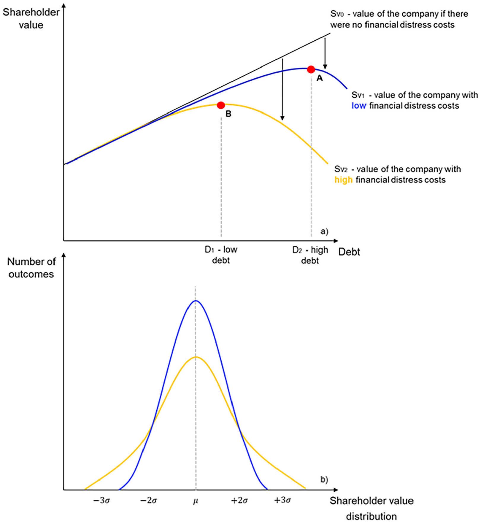
Optimal debt levels and shareholder value for projects with different levels of cash-flow volatility and financial distress costs. (a) a company with less volatile revenues will experience financial distress less frequently, leading to lower costs of liquidity management and financial distress (blue), as opposed to a company with more volatile revenues (yellow). Accordingly, their optimal debt levels, shown at points A and B, would differ. (b) greater revenue volatility will lead to shareholder returns that are more dispersed around the mean (yellow), as opposed to a company with lower levels of cash-flow volatility (blue).
2.2 Financial Distress and Project Financing
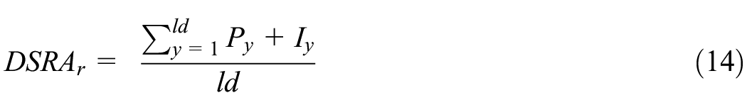
Although trade-off theory primarily deals with corporate finance settings, we apply its basic principles and adjust it to a single-project company or project financing. The first sign of financial distress in project financing is the violation of debt covenants (Asquith, Gertner and Scharfstein 1994; Baldwin and Mason 1983). Debt covenants are financial and non-financial restrictions that a lender places on a borrower to maintain the financial sustainability of the loan agreement (Gatti, Caselli and Steffanoni 2012). For instance, lenders frequently require the borrower to maintain a Debt Service Reserve Account (DSRA) worth between six and twelve months of debt service (Bodmer 2014) to be drawn on if the borrower fails to service debt in the short term due to temporary and unexpected events. In addition, they usually impose financial covenants like a debt service coverage ratio requirement
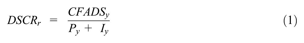
In renewable energy financing, lenders couple the
Within our model, we differentiate between the financing conditions of the merchant and the CfD-backed project to replicate the lenders’ anticipated response to these two different revenue risk profiles. While referring back to Figure 1, we expect that the merchant project will experience financial distress more frequently and require more cash liquidity to avoid violating debt covenants than the CfD-backed project because of its greater cash flow volatility. Therefore, the merchant project would maximize shareholder value at a lower debt level than the CfD project. We developed a modeling framework that quantifies the costs of financial distress to test this hypothesis, as explained in the next section.
3. Methods
3.1 Overview of the Modeling Approach
When estimating the financial viability of an offshore wind farm, expected electricity production and electricity prices play a crucial role. To model project cash flows, lenders typically purchase power-price forecasts from data providers or power-market consultants (Raikar and Adamson 2020). However, such forecasts are a large source of uncertainty due to their underlying assumptions, which are not publicly available. As illustrated in Figure 2, we address this gap by extending a stochastic power price and wind feed-in model (Keles et al. 2013) to calculate revenues for an offshore wind farm.
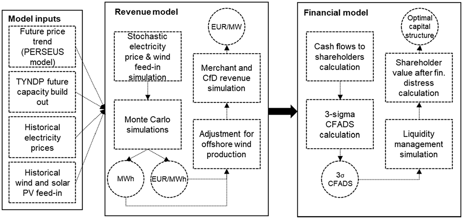
Overview of the methodology.
The Keles et al. (2013) stochastic price model generates yearly price time series, which is insufficient for modeling long-term revenues spanning the thirty-year lifespan of an offshore wind farm. To address this limitation while retaining price stochasticity of Keles et al. (2013)—a critical component of our financial distress analysis—we model yearly time series around future annual mean prices at five-year intervals from 2020 to 2050, generating 1000 scenarios for each time step. These prices are derived from PERSEUS-EU (Yilmaz et al. 2022)—a constrained linear optimization model—representing one of many possible price projections. Nonetheless, they provide a plausible depiction of the European energy system and include country-specific price estimates, such as for Germany.
The PERSEUS-EU prices enable the creation of a yearly price time series at levels consistent with expected power system prices. We incorporate future solar and wind capacity additions to account for the price volatility caused by an increasing share of intermittent renewables. We model the impact of these through the in-built Merit Order Effect in the Keles et al. (2013) price model. Therefore, in our price modeling, the generated electricity prices are aligned with expected renewable feed-in levels, resulting in lower prices during high wind and solar PV output periods and higher prices when renewable production is low. Additionally, the model outputs wind production for the entire German wind fleet. To ensure accuracy, we adjust this production profile to reflect the specific generation characteristics of an offshore wind farm in the North Sea.
Next, we build upon Kitzing and Weber’s (2015) liquidity management model, initially developed for a corporate financing setting, to quantify financial distress. As indicated in Figure 2, we develop a model for project financing and reshape the liquidity management module to quantify financial distress as the additional cash liquidity required in periods when the sponsors violate debt covenants, including a DSCR requirement and a Debt Service Reserve Account (DSRA) worth twelve months of debt service. We account for the probability of default by benchmarking the Cash Flow Available for Debt Service (CFADS) 1 of each revenue scenario with a three-sigma CFADS level for debt levels between 40 percent and 90 percent 2 in 5 percentage point steps. Finally, we calculate the project’s optimal capital structure by finding the debt size that maximizes equity holders’ returns or shareholder value within the 40 percent to 90 percent debt size range. We present the two model segments in greater detail in the following sections.
3.2 Revenue Model
The revenue model first simulates the electricity prices and offshore wind production, followed by the CfD and merchant offshore wind project revenues. We proceed by outlining each of these segments in the following sections.
3.2.1 Electricity Price Simulation
In most power markets worldwide, electricity prices are characterized by daily and weekly cycles, high volatility, mean reversion, and frequent price spikes. Many different models can be applied to simulate such variability and reproduce the electricity market merit order—an electricity supply curve created by ranking generators according to their short-term marginal costs (SRMC) (Sensfuß, Ragwitz and Genoese 2008). Econometric time-series models, such as the autoregressive moving average (ARMA) and mean-reversion process, have been used extensively for electricity price simulations (Andreis et al. 2020; Billé et al. 2023; de Oliveira, Mandal and Power 2019; Gudkov and Ignatieva 2021; Lucic and Xydis 2023; Mestre et al. 2020; Yu 2022). Such models simulate the deterministic and stochastic components of historical electricity prices to create short-term price projections and have been shown to replicate historical prices with the smallest simulation errors (Keles et al. 2012). While mean-reversion models have been extended to consider electricity price volatility (Escribano, Peña and Villaplana 2011; Eydeland and Wolyniec 2003), they lack a good representation of seasonality and price cycles (Swider and Weber 2007). In contrast, the ARMA model simulates time-dependencies within a time series, thus modeling short-term price movements better. Furthermore, electricity prices jump from their base regime to other jump regimes and remain there for several hours, for instance, during price spikes. The model used by Keles et al. (2013) simulates these characteristics by combining the ARMA model with regime-switching elements (Weron 2009) and accounts for the merit-order effect leading to lower power-market prices in times of high wind and solar PV feed-in (Sensfuß. Ragwitz and Genoese 2008).
We model hourly electricity prices and wind feed-in for the German power system. The model first excludes the merit-order effect through a least-square regression of electricity prices with respect to wind power feed-in

This generates coefficients

Since modern offshore wind farms have around thirty years of lifetime (Danish Energy Agency 2020), financial models must consider long-term price trends. As discussed earlier, we correct

While we have considered the future merit order effect of the renewables in this modeling approach, we do not include the price effect energy storage can have on the inner-day/year price resolution. They might reduce the price volatility to a certain extent. However, as they will mostly replace other peaking technologies, such as gas turbines, and will follow the bidding behavior of these alternative technologies, their price impact is likely similar to that of the replaced gas turbines, which we implicitly account for with the input data we use.
In parallel with simulating electricity prices, the model follows similar deseasonalization and resesonalization procedures to generate wind feed-in time series
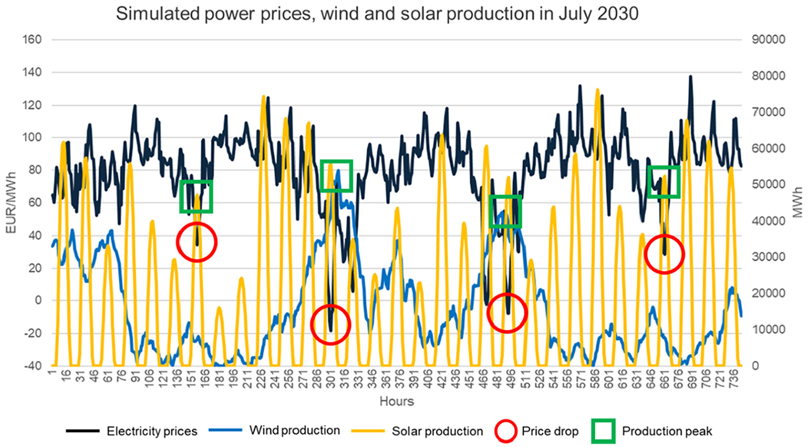
Simulated electricity prices and wind and solar PV production for the high-price scenario in July 2030.
Our model derives 101 TWh of production from solar PV and 203 TWh from wind energy in 2030, compared to 100 TWh and approximately 250 TWh in the German Green Deal scenarios (European Commission 2021). The lower modeled wind production implies that fewer negative prices are generated during periods of high wind production, meaning the price reductions in Figure 3 would have been more pronounced. However, the more extensive price drops would imply an even stronger role of two-sided CfDs in mitigating price risks, supporting the main research question of this study. We provide a more detailed comparison of our results, including assumed installed capacities, modeled production, and the resulting fleet-wide capacity factors in Tables A1 to A3 in the Annex.
3.2.2 Offshore Wind Production Simulation
To account for differences between the production from the entire wind fleet and an individual offshore wind farm, we adjust the output
Since
where

We derive the upscaled capacity factors
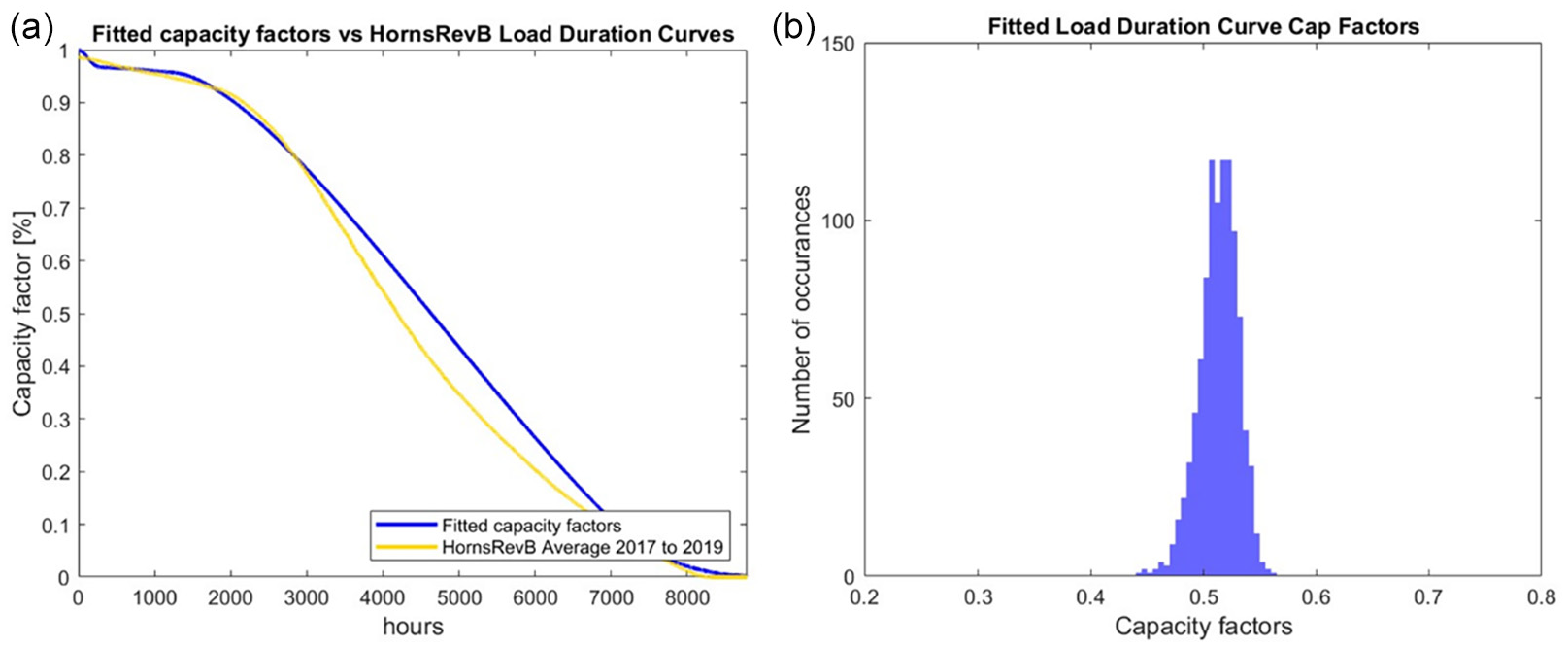
(a) Load duration curves for Horns Rev B versus simulated offshore wind production and (b) Simulated hourly capacity factors. Both images represent averages for all the simulated years.
3.2.3 Revenue Simulation
We derive the electricity prices and offshore wind production in each time-step
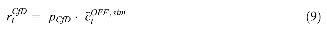

where
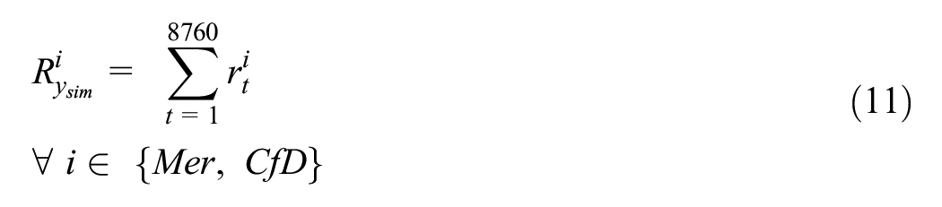
Following this, we then interpolate the revenues between the eleven simulated years and derive thirty-year revenue curves
Herein, we simplify the CfD and merchant revenue calculations in several ways. First, regulators determine the CfD payments by comparing the bid level with a reference price calculated over a pre-defined period. For instance, Denmark’s CfD references payments to the previous year’s average spot electricity prices (Danish Energy Agency 2020), while the German sliding premium applies one month as the reference period (Klobasa et al. 2013). Therefore, the generator’s revenues depend on its periodic trading activity and can exceed or fall short of the reference price. Here, we assume an hourly referencing period, reflecting the CfD design applied in the UK (CEER 2016). Besides the simplicity of calculating revenues for such a CfD—as highlighted in the Introduction—this design also decreases price risk the most (Kitzing et al. 2024).
Second, Germany’s new Renewable Energy Act suspends all support payments when the spot-market price is negative for four consecutive hours to avoid excessive electricity production during those times (BMWi 2020). Although our study assumes an offshore wind project in the German North Sea, we disregard this rule to simplify. Third, our framework does not assume the wind farm stops generating electricity and selling for merchant prices when prices are negative. Arguably, our assumptions deviate from actual offshore wind farm electricity marketing, where production would be halted in negative hours. We subsequently calculate the effect of these simplifications on revenues and elaborate on their implications on optimal debt size in the Results section. Third, to highlight the differences in financial distress between the CfD and merchant revenues, we assume full merchant revenues instead of assessing mixed structures where projects have CfDs or corporate PPAs for part of their lifetimes and a merchant tail thereafter (Gohdes et al. 2023).
3.2.4 CfD Bid Estimation
The CfD bid level directly impacts the project’s financial distress and shareholder value and is crucial in the project sponsor’s negotiations with banks regarding financial terms, including the debt size. Besides financial aspects, the CfD level affects project profitability or net present value (NPV), unlike the merchant case, whose NPV is mainly determined by the assumed electricity price scenario. Our analysis assumes that a single project sponsor chooses between the CfD and merchant cases. Therefore, to make the selection between the two cases comparable from the single-investor perspective, we first have to calculate the CfD bid levels that lead to the same NPV as the equivalent case with merchant revenues at each debt level. This approach eliminates profitability as the primary decision criterion—since the NPV remains comparable between the two projects—and instead highlights revenue volatility as the key factor in decision-making. Considering this, we calculate in 5 percent debt level steps
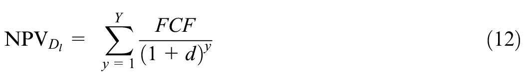
where
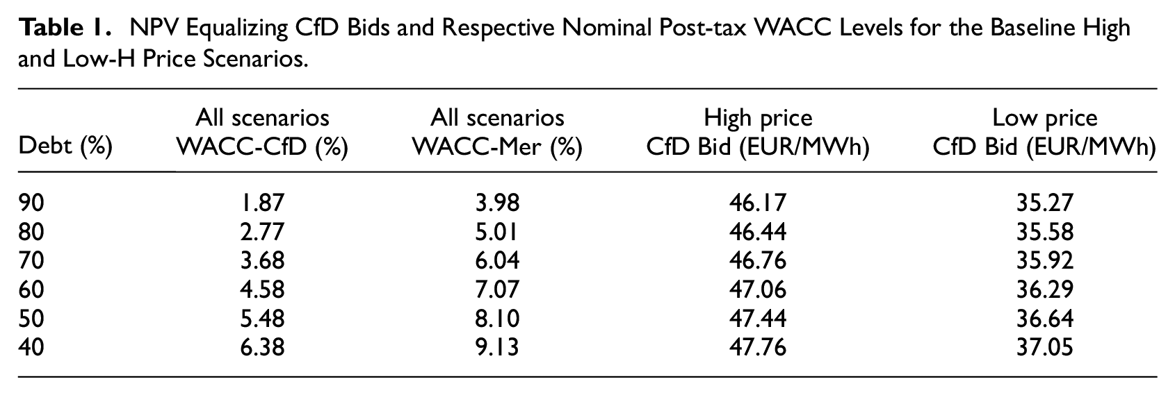
NPV Equalizing CfD Bids and Respective Nominal Post-tax WACC Levels for the Baseline High and Low-H Price Scenarios.
3.3 Financial Model
We use the derived revenues
3.3.1 Cash Flows to Shareholders Before Financial Distress
We expand upon Bodmer (2014) project-financing set-up to construct the financial model. We calculate cash flows to shareholders before financial distress
Cash-Flow Statement.
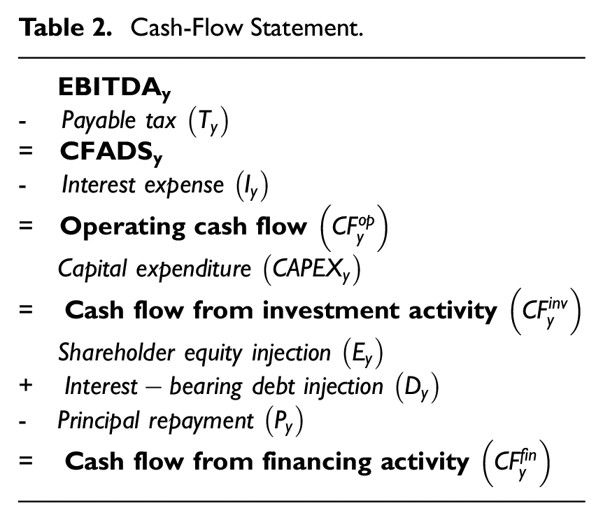
After obtaining the three separate parts of the cash-flow statement, we derive

When calculating the project’s interest and principal payments, we assume an annuity-repayment structure, requiring the borrower to pay the lender a fixed annuity composed of the interest and principal in each debt repayment period (Yescombe 2013). We calculate the initial loan amount as the multiple of the project’s capital expenditures (CAPEX) and the exogenously determined debt size, expressed as the percentage of debt in total CAPEX.
3.3.2 Liquidity Management Module
We develop a liquidity management calculation adjusted to account for financial distress from a project financing perspective. Kitzing and Weber (2015) define a liquidity account
We then apply
Liquidity Management Module.
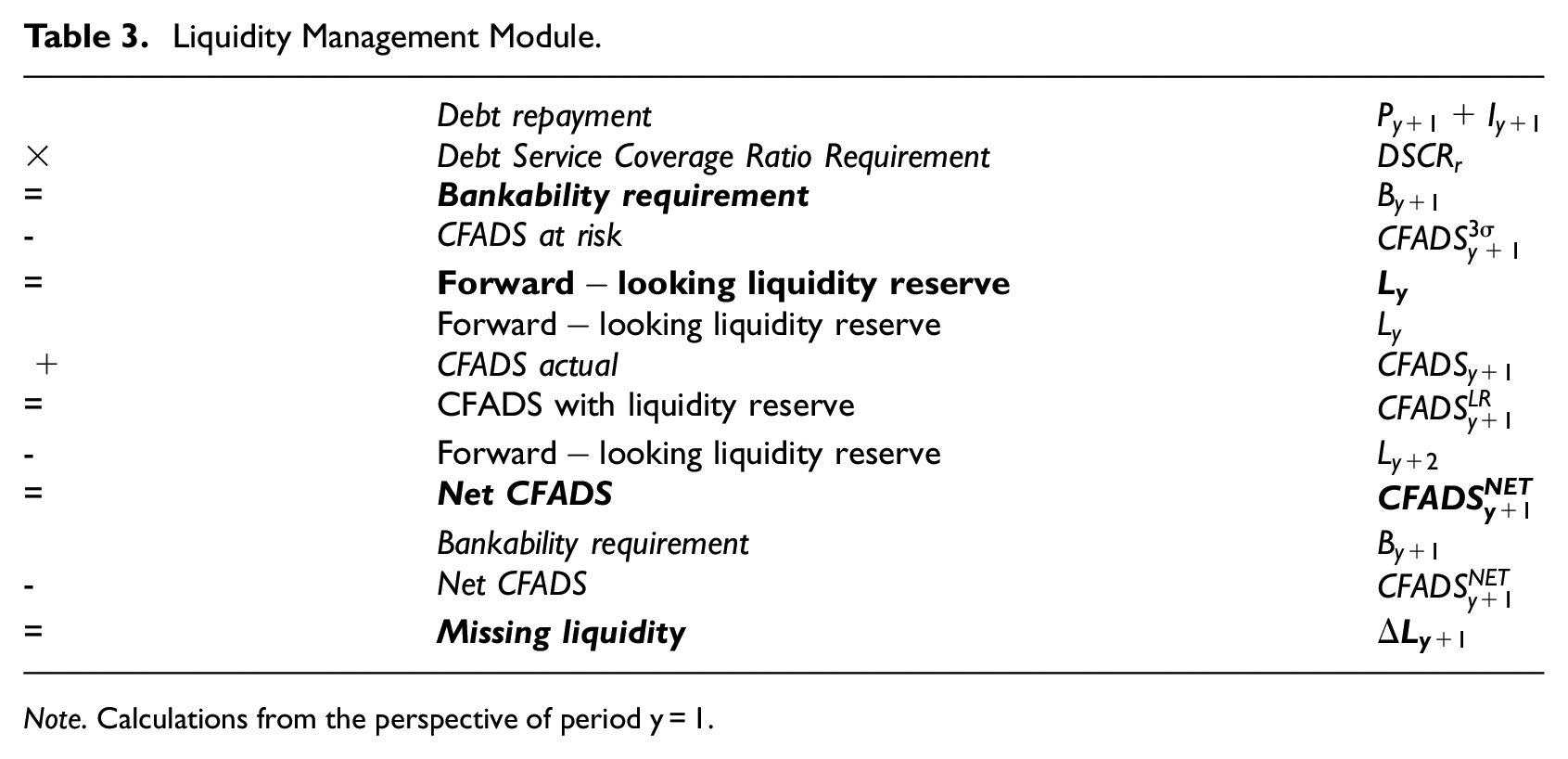
Note. Calculations from the perspective of period y = 1.
3.3.3 Shareholder Value After Financial Distress
We pass the
where
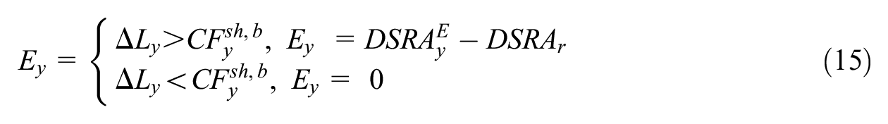
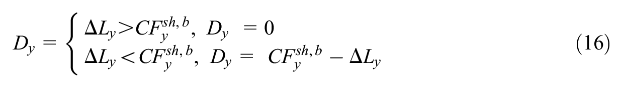
Therefore, the cash flows to shareholders after financial distress
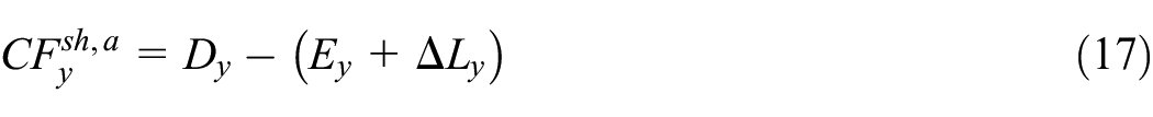
Next, to obtain shareholder value after financial distress
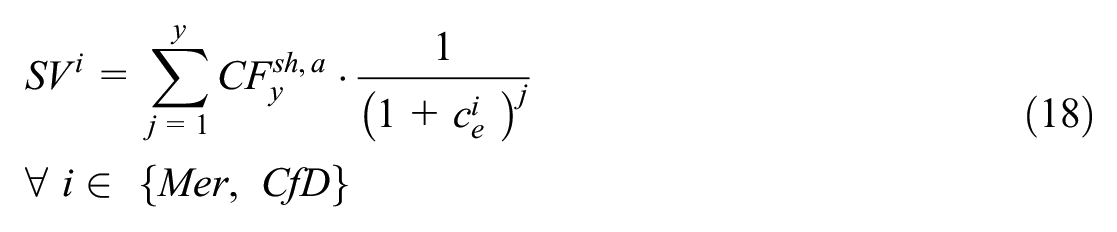
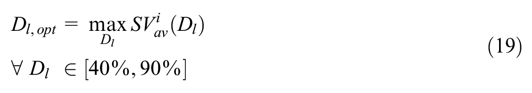
Finally, to find the optimal debt level, we first average
To determine whether the number of Monte Carlo sampling runs we conduct are sufficient, we conduct a test following Winston (2001). 6 We test the number of required runs at 90 percent and 70 percent debt levels for both the high- and low-price situations and the CfD and merchant projects. The resulting required Monte Carlo simulations vary between 70 and 82 for the CfD and 437 and 217 for the merchant project in the case of the high-price scenario and the two debt levels, respectively. The numbers are higher for the low-price scenario, with 454 and 147 simulation runs for the CfD and 827 and 811 for the merchant project for the two respective debt levels. These tests prove at a 95 percent confidence level that conducting 1,000 simulation runs is sufficient.
3.4 Input Data and Scenarios
The generated electricity prices are in real values (see Yilmaz et al. 2022). Hence, we conduct the analysis in real terms, as presented in Table 4, outlining the investment assumptions. Furter, we analyze the offshore wind project on a per MW basis to achieve easier general applicability of results. Next, we assume the same access to the grid connection and seabed for both the CfD and merchant project, including the grid connection paid for by the grid operator and no sea-bed lease payments. Regarding financing conditions, we apply debt levels and project financing conditions from a financing survey that includes offshore wind in Germany, Belgium, France, and the UK (Roth, Đukan et al. 2021). As shown in Table 5, we assume that commercial banks would apply more stringent financing terms for the merchant case, applying a higher DSCR, shorter loan duration and larger interest rate. Further, in alignment with the literature, we also assume the project sponsor would apply higher equity costs to the merchant project than in the CfD case (Gohdes et al. 2022). We derive the cost of equity via the Capital Asset Pricing Model (Lintner 1965; Sharpe 1964) using re-levered equity beta values for a CfD and merchant offshore wind farm based on European Economics (2018), and a respective risk-free rate and expected return on the German market, as indicated in Table 5.
Investment Inputs for the Model (2020 Real Values).
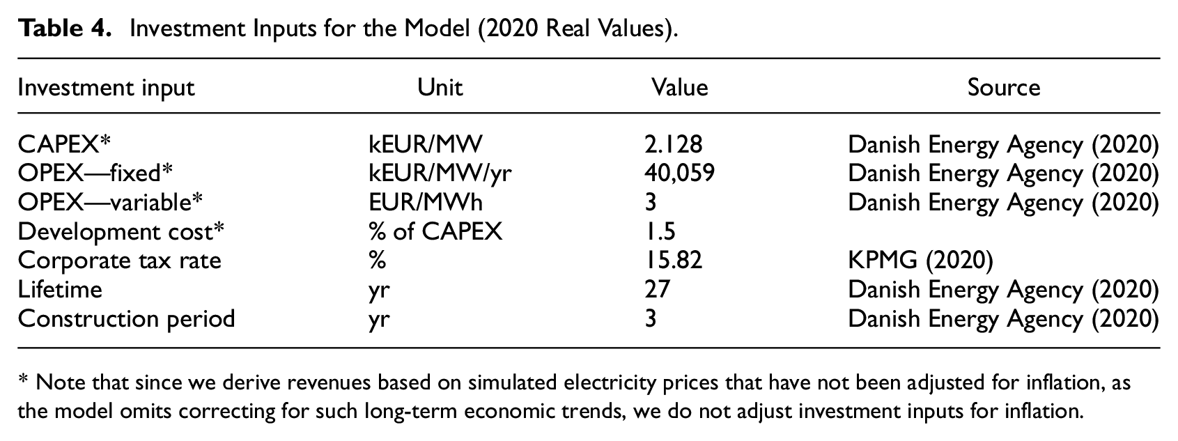
* Note that since we derive revenues based on simulated electricity prices that have not been adjusted for inflation, as the model omits correcting for such long-term economic trends, we do not adjust investment inputs for inflation.
Financing Conditions for the Base Merchant and CfD Cases, Based on Surveyed Financing Conditions for Offshore Wind in Germany, Belgium, France, and the UK.
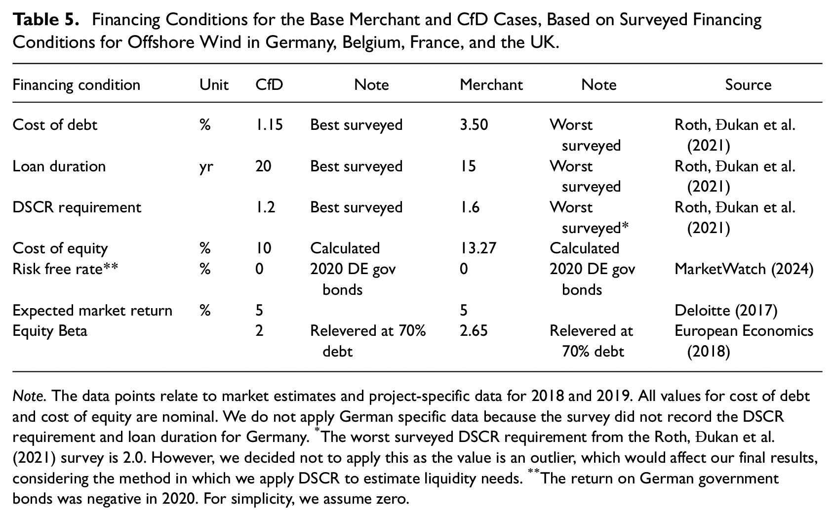
Note. The data points relate to market estimates and project-specific data for 2018 and 2019. All values for cost of debt and cost of equity are nominal. We do not apply German specific data because the survey did not record the DSCR requirement and loan duration for Germany.
The worst surveyed DSCR requirement from the Roth, Đukan et al. (2021) survey is 2.0. However, we decided not to apply this as the value is an outlier, which would affect our final results, considering the method in which we apply DSCR to estimate liquidity needs.
The return on German government bonds was negative in 2020. For simplicity, we assume zero.
Combined, these financing conditions make up the CfD and merchant WACC levels. We use a post-tax real WACC as the discount rate. Since the Roth, Đukan, et al. (2021) data is nominal, we first calculate the nominal post-tax WACC by following Steffen (2020) as:

where
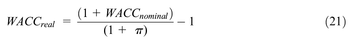
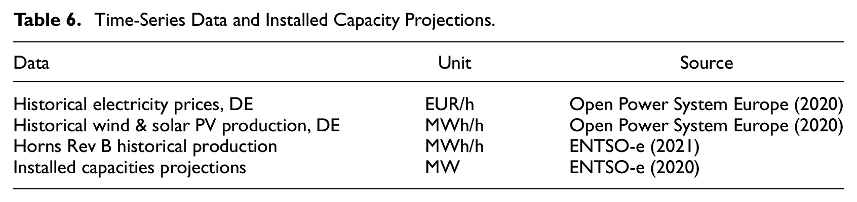
We repeat this procedure to derive the real cost of equity. Further, regarding the time-series data and installed capacity projections, we apply the data shown in Table 6.
Time-Series Data and Installed Capacity Projections.
Further, we apply the results for two long-term electricity price scenarios that examine Germany’s future power system from the perspective of two different increasing carbon allowance price paths. Yilmaz et al. (2022) generate High and Low scenarios, as shown in Figure 5. Instead of conducting the simulation for the Low-price scenario, we calculate another hypothetical scenario with even lower prices, leading to only 50 percent of the price increase shown in the Low price path, as depicted by the yellow line in Figure 5. Doing this enables us to simulate various outcomes regarding financial distress and capital structure. We derive this hypothetical Low price path or Low-H by deducting the difference between the High and Low scenarios from the Low-price path. The applied prices assume a carbon price projection of 140 USD per ton in 2040 (expressed in real 2015 values) (Yilmaz et al. 2022). Finally, the Yilmaz et al. (2022) model assumes perfect foresight, ensuring full recovery of all capacity investments. Consequently, the resulting electricity prices reflect this setup and guarantee cost recovery.
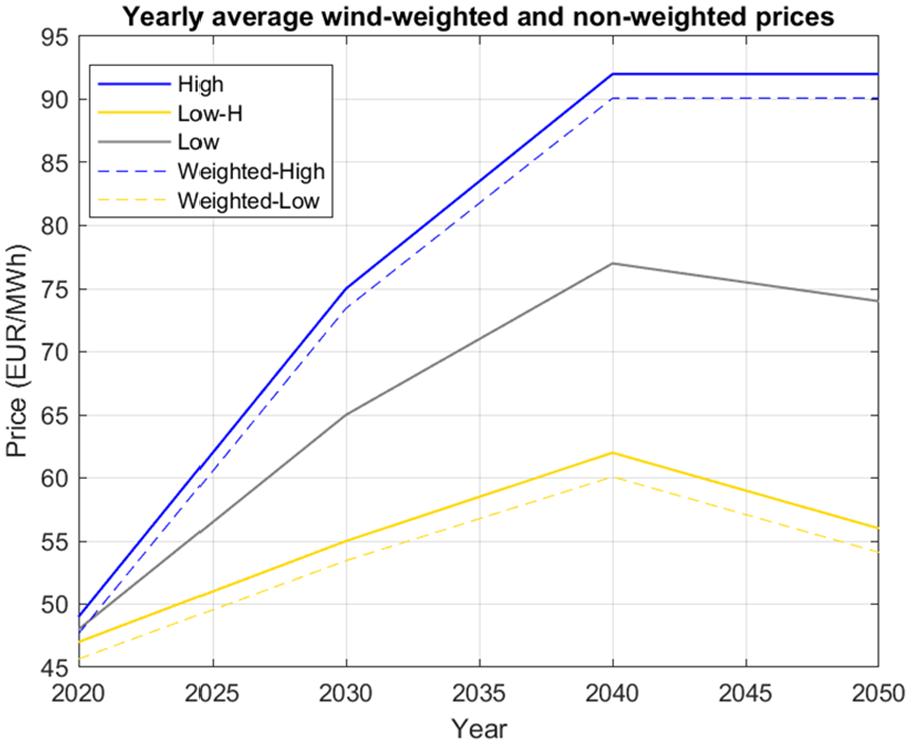
Assumed electricity price scenarios for the period between 2020 and 2050.
In addition to the long-term scenarios, Figure 5 also displays the price duration curves, including the wind-weighted prices for the two scenarios we implement. To present the prices in more detail, we show the 2020 to 2050 weighed and non-weighed hourly prices for the Low-H scenario in Figure 6. We weigh the hourly prices with a weekly capture price, calculated following Hirth (2013). In addition, we show the price duration curves for the High price scenario in Figure A2, and the weekly mean weighted and non-weighted prices for both scenarios in Figures A3 and Figure A4 in the Annex.
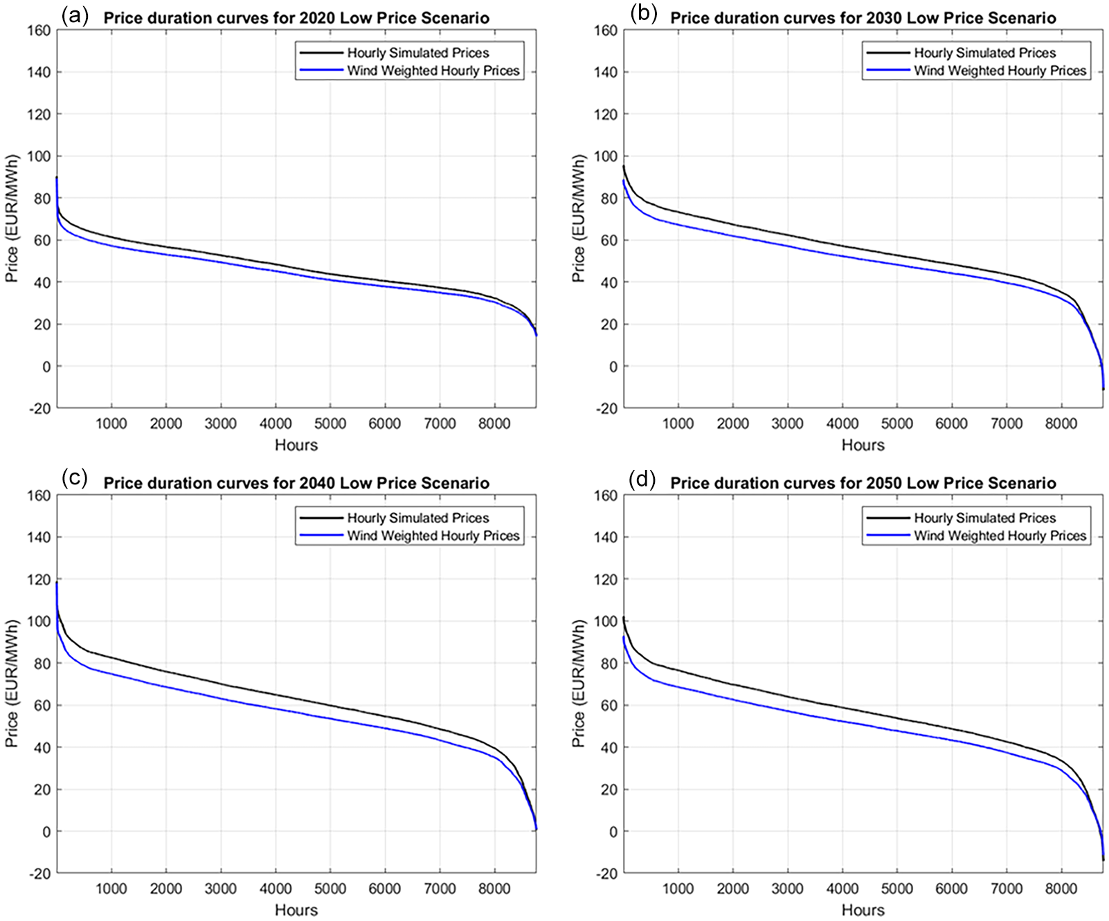
Wind-weighted and non-wind-weighted price duration curves for the low price scenario for the years (a) 2020, (b) 2030, (c) 2040, and (d) 2050. The presented curves are means of all scenarios.
4. Results
4.1 Shareholder Value and Financial Distress Costs in the Base Scenarios
Figure 7 presents the main outcome of our study, showing shareholder values (panels a and b) and financial distress costs (panels c and d) at different debt sizes. The results show that a project backed by a two-sided CfD contract would, on average, achieve between 27 and 15 percentage points higher debt shares than in the merchant case. As Figure 7a indicates, in the high-price scenario, the CfD maximizes shareholder value at the highest measured debt size of 90 percent, while the merchant project does so at a 74 percent debt size. Regarding the low-price scenario, both projects maximize shareholder value at lower debt sizes, the CfD project at 77 percent and the merchant at 50 percent, as shown in Figure 7b. Lower prices reduce revenues and CFADS, leading to more frequent financial distress, especially for the merchant project. These results are for derived bids that equalize the NPV of the CfD and merchant projects (see Section 3.2.3) ranging from 46.17 EUR/MWh to 47.76 EUR/MWh for debt sizes between 90 percent and 40 percent in the high price scenario and between 35.27 EUR/MWh and 37.05 EUR/MWh in the low-price scenario. All the bid levels and the respective WACC values or discount rates for each debt size are presented in Table 1. 7
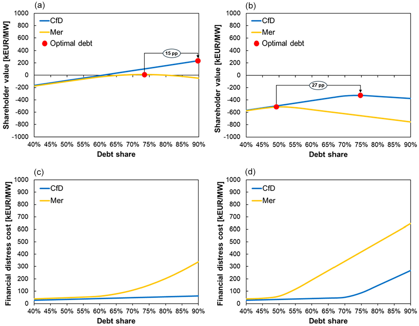
High and low price base results. Graphs (a) and (b) show average shareholder values at individual debt sizes between 40 percent and 90 percent for the CfD (blue) and merchant (yellow) projects in the high and low price scenarios, respectively. Graphs (c) and (d) show financial distress costs for the two projects.
Several other findings arise from Figure 7. First, panels a and b show that the CfD project almost always has higher shareholder value than the merchant project, except at lower debt levels where they are almost identical. At higher leverage, the CfD case leads to lower financial distress, as shown in panels c and d, protecting shareholders from market price volatility. Second, low power prices lead to shareholder values below zero for both the CfD and merchant projects, indicating that under these price and CfD bids (see Table 1), shareholders would not support the projects in practice, stressing the importance of power price risks. Figure 8 further stresses the power risk hedging benefits of CfDs by showing the distribution of mean shareholder values for the two price scenarios at debt levels where their shareholder values are almost the same. In both power price scenarios, the CfD project achieves lower standard deviation of shareholder values than the merchant case, especially in the low price scenario.
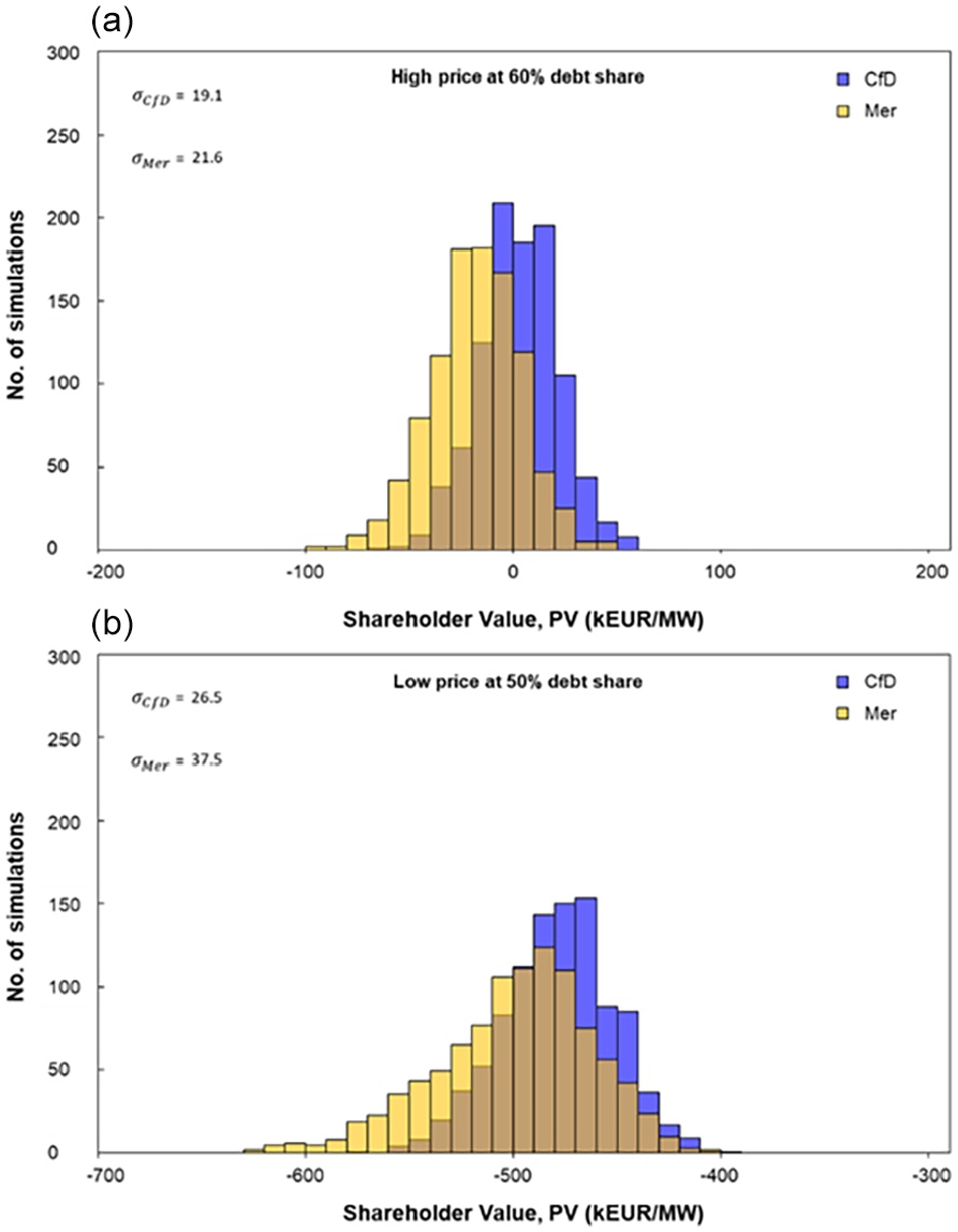
Distribution of shareholder value in the high and low price cases at debt sizes where the shareholder values are equal or nearly equal, as in the case of low prices. These shareholder values hold for post-tax nominal WACC values of 3.4 percent and 5.7 percent for the CfD and merchant cases in the high price scenario and at 60 percent debt, and 4.13 percent and 6.71 percent at 50 percent debt for the low-price scenario and the two price scenarios, respectively. (a) Distribution of shareholder value in the high price case values of 3.4% and 5.7% for the CfD and merchant cases and at 60% debt. (b) Distribution of shareholder value in the low price case values of 4.13% and 6.71% for the CfD and merchant cases and at 50% debt.
These results resemble the theoretical framework we presented in Figure 1. We show that greater cash flow volatility reduces optimal leverage, which aligns with earlier research (Keefe and Yaghoubi 2016; Minton and Schrand 1999). A larger debt size increases the project’s debt service relative to its cash flows, making the violation of debt covenants more likely and financial distress more frequent in the case of volatile revenues. Our estimated optimal debt sizes correspond with survey findings of financing conditions within the EU, which find debt shares for offshore wind ranging between 70 percent and 85 percent for projects in Germany, Belgium, France, and the UK (Roth, Đukan et al. 2021).
4.2 Sensitivity Analysis
The above results depend on several key assumptions, including the assumed CfD design regarding support payments during times of negative prices and variations in financing conditions. Here, we stress-test our model against these inputs.
4.2.1 Impact of Negative Price Rules
Our results would vary slightly depending on the CfD design and merchant revenue rules applied. We demonstrate the impact for the low-price scenario since it has a higher frequency and duration of negative electricity prices (see Figure A9 in Annex). Implementing the four-hour price rule would decrease CfD revenues by 0.04 to 1.35 percentage points (pp) for the years 2020 and 2050 (see Figures A5 and A6 in the Annex), while for the merchant project revenues would increase between 0.09 and 1.9 pp when assuming no sales at negative power prices (see Figures A7 and A8 in the Annex). Under the assumption that we implement the merchant revenue rules of no sales for negative prices and the four-hour CfD rule and omit findings NPV-equalizing CfD bids (assuming the same bids as for the baseline case), the optimal debt size would decrease by 0.35 pp for the CfD project and increase by 0.44 pp in the merchant case in the low-price scenario. In conclusion, the difference in revenues between our baseline case and revenue rules that consider negative prices is small and does not exhibit a large impact on the results.
4.2.2 Impact of Financing Conditions
To investigate the magnitude impact of financing drivers on debt size, we change the financing conditions individually by 20 percent from their base values, as shown in Table 7. Besides this, we vary all the financing conditions simultaneously to the average values between the CfD and merchant bases cases. We conduct each scenario for debt sizes between 40 percent and 90 percent in 5 percent steps. 8 Figure 9 shows the debt sizes that maximize mean shareholder value after financial distress for each sensitivity run and the base cases. As each sensitivity run changes the merchant project’s NPV, we estimate the NPV-equalizing CfD levels for each run, as outlined in Section 3.2.3.
Sensitivity Analysis Assumptions.
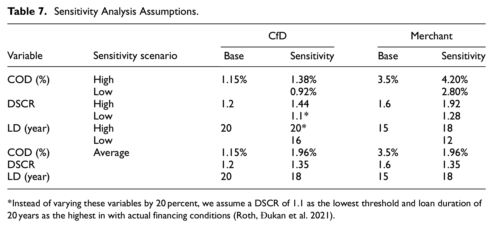
*Instead of varying these variables by 20 percent, we assume a DSCR of 1.1 as the lowest threshold and loan duration of 20 years as the highest in with actual financing conditions (Roth, Đukan et al. 2021).
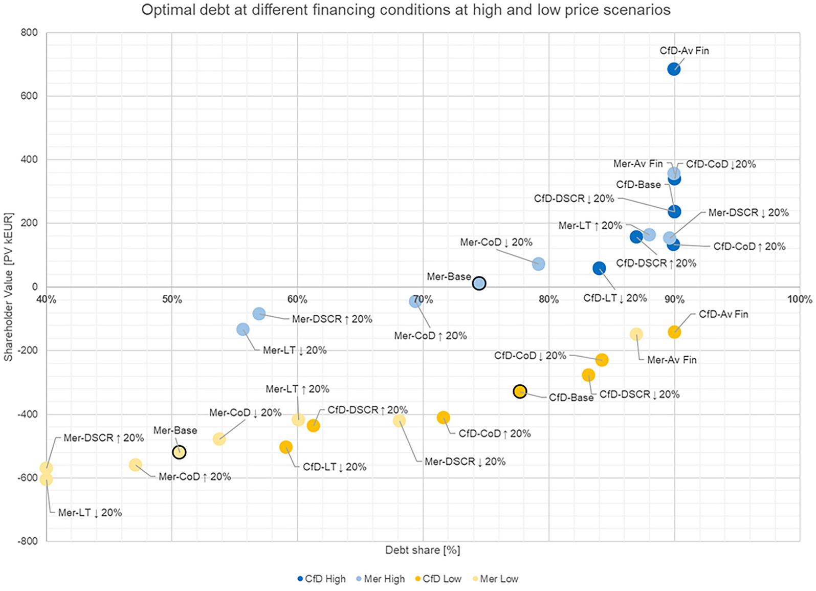
Results of the sensitivity analysis.
We draw several main observations from Figure 9. First, the CfD project delivers higher optimal debt sizes than the merchant case in both the low and high-price scenarios, regardless of the changes in financing conditions, as outlined by the dark blue and yellow points. Second, the CfD level and power prices scenarios have a large impact on leverage. Within the low-price scenario, we assume lower CfD levels, leading to a smaller cash buffer and a higher frequency of financial distress situations. In contrast, the higher bid levels and a merchant tail with larger power prices lead to lower sensitivity of CfD projects to changes to financing conditions in the high-price scenario.
Third, the results are most sensitive to DSCR requirements and loan duration changes and the least sensitive to changes in debt costs. Varying the DSCR requirement and loan duration leads to an average 12 percentage points change in debt size for both projects and power price scenarios. However, in some cases, the variations are greater. For instance, in the high-price scenario, reducing the DSCR requirement for the merchant project from 1.60 to 1.28 increases leverage from 74 percent to the highest measured debt level of 90 percent. Fourth, we observe the most significant changes in optimal debt levels when changing the DSCR requirement combined with loan duration and cost of debt. For instance, a 1.35 DSCR requirement combined with an 18-year loan duration and a 1.96 percent interest rate leads to an optimal debt size of 87 percent for the merchant project, compared to the base level of 51 percent in the low-price scenario.
Overall, changes to financing conditions have a much larger impact on optimal debt size than CfD design rules and merchant revenues that account for negative prices. Furthermore, our results indicate that debt covenants and loan duration are the main drivers of leverage, whereas debt interest rates have a smaller impact. These results align with the financing industry, such as Standard & Poor’s recommendations to increase the DSCR requirement in response to adjusting lender exposure to merchant power plants (Rigby 1999) instead of increasing debt margins, which are more exposed to external influences such as changing macroeconomic conditions (Egli, Steffen and Schmidt 2018; Schmidt et al. 2019).
4.3 Implications of Revenue Stabilization
The implications of our findings go beyond the financing of individual projects. The positive impact of revenue stabilization via two-sided CfDs increases leverage and reduces the project’s WACC, leading to lower electricity production costs and consumer benefits. Figure 10 shows the impact on real LCOE for the high- and low-price scenarios (for the LCOE calculation method, refer to Section “Levelized Costs of Electricity” in the Annex). We subsequently adjust the debt level from its highest level in the CfD case to the optimal debt size we derive in our analysis for the baseline merchant cases (shown in red) and then change the project’s interest rate and cost of equity to that of the merchant case (shown in gray). Figure 10 panels a and c, demonstrate that assuming merchant debt levels, instead of the optimal CfD debt increases the real LCOE by between 4 EUR/MWh and 8 EUR/MWh for the two price scenarios, which, combined with changing interest rates and costs of equity from those assumed under the CfD case to the merchant case level, increase overall LCOE by between 12 and 19 EUR/MWh for the high and low price scenarios, respectively. Assuming merchant revenues instead the CfD increases the real post-tax WACC by between 1.4 pp and 2.4 pp, depending on the price scenario, as shown in Figure 10 panels b and d. Our results provide a rough indication of the benefits to society, where state-led revenue stabilization decreases electricity generation costs, in turn for governments taking on the risk hedging role.
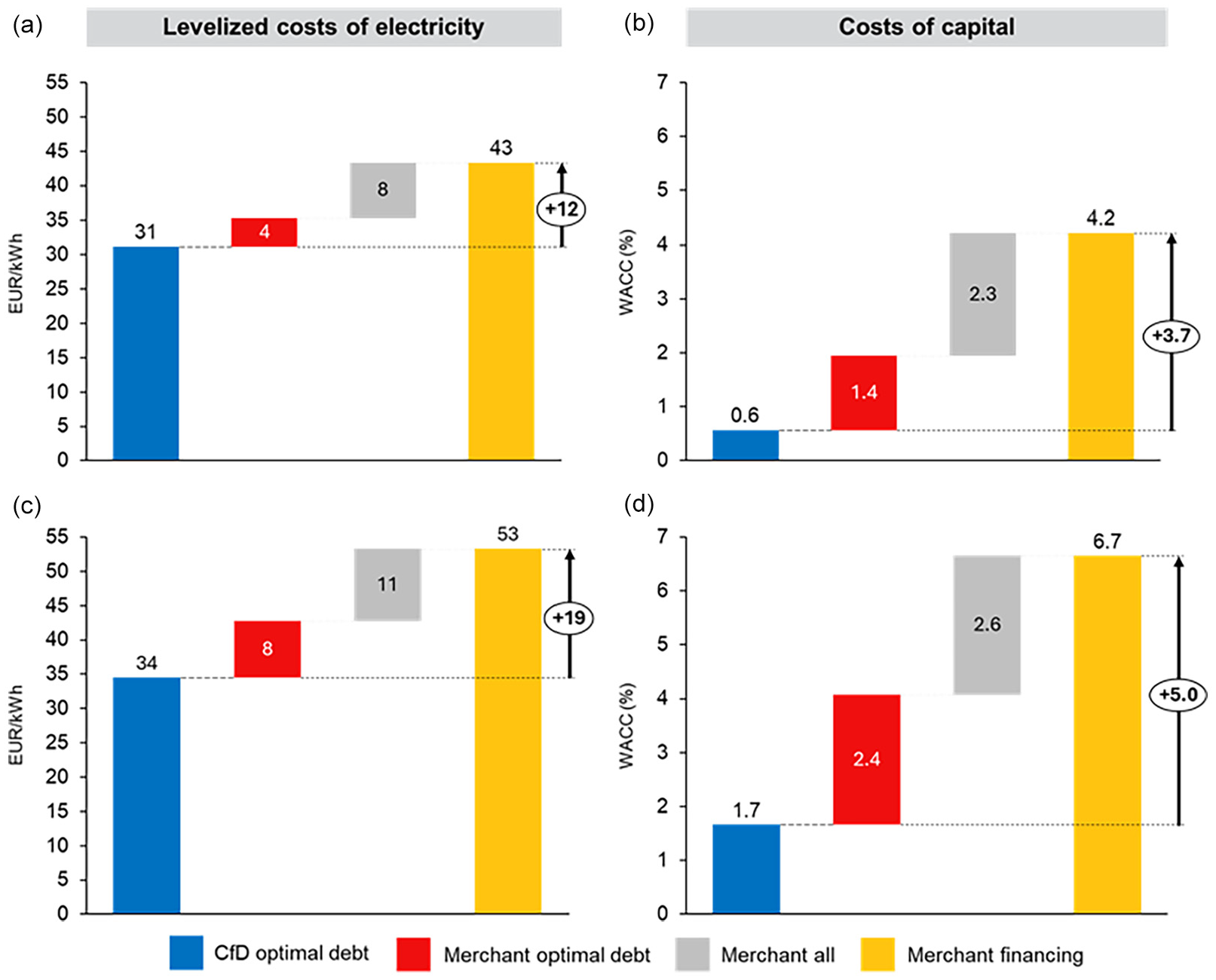
The impact of two-sided CfDs on LCOE and costs of capital: (a and b) high price and (c and d) low price.
5. Critical Reflection and Discussion
Our study is the first to quantify the impact of merchant risk and revenue stabilization via CfDs on financial distress and debt sizing, adding to the dynamic discussion on CfD designs (Kitzing et al. 2024). Nevertheless, there are several considerations regarding our study. First, we assess the impact of revenue stabilization via power purchase contracts. Notwithstanding other revenue risk mitigation mechanisms such as forward electricity contracts (Woo, Horowitz and Hoang 2001) and option hedging involving financial settlements with financial counterparts (Guidera and Jamshidi 2016), PPAs are the backbone of renewable energy financing. The question is who should bare the cost of risk mitigation. Our study assesses government-backed CfDs; however, other PPA mechanisms, such as contracts with corporates, exist in various forms (Bruce et al. 2020; Tang and Zhang 2019) and have been growing by 65 percent year on year since 2013 (Bruce et al. 2020). Relying on corporate PPAs to deliver renewable energy capacity could replace the risk-mitigation role assumed by CfDs and save public finances (Gohdes et al. 2023).
Government-held auctions are administrative processes, and as such, they might be organized inefficiently and lead to sub-optimal outcomes such as not procuring sea bed rights for the least cost or to the counterparty most capable of delivering the project in time (Mora et al. 2017). While there is empirical evidence for this (see for instance, Winkler, Magosch and Ragwitz 2018), it does not imply that corporate PPAs could completely substitute government-procured CfDs. The main reason is the capacity of the corporate PPA market to mitigate power price risks for the volume of offshore wind electricity Europe plants to deploy until 2050. Corporates with investment-grade credit ratings (above BBB- or Baa3, depending on the credit agency) and high and long-term demand for green electricity are limited in supply (Beiter et al. 2023), making the financing of offshore wind farms contracted via corporate PPAs more expensive (Gohdes et al. 2022; Hundt, Jahnel and Horsch 2021). Furthermore, through organizing CfD auctions, governments control the renewable capacity build-out and provide incentives even when market conditions increase the cost of corporate procurement, such as supply chain bottlenecks and rising materials costs (IEA 2023).
Second, implementing two-sided CfDs could have implications for energy markets, which go beyond the main research question of this study. Two-sided CfDs could enable easier access to financing offshore wind projects and, hence, a more active offshore wind market. Besides utilities and oil & gas companies, the biggest investors in offshore wind in Europe (Đukan et al. 2023), higher revenue stability could attract investors with more conservative risk-return investment profiles, such as pension funds and insurance companies. The enhanced actor diversity might reduce the sector’s cost of capital, helping offshore wind become more cost-competitive. These institutional investors could invigorate project acquisitions and capital refinancing back into project developers’ balance sheets, a model known as farm-downs (McKinsey & Company 2020). On the other hand, greater offshore wind penetration could induce revenue cannibalization as the ever-growing wind fleet suppresses electricity prices due to its correlated production profile (Hirth 2013). While the two-sided CfD would hedge project owners against price drops (depending on negative price designs), it could suppress prices for other generators like solar PV (López Prol, Steininger and Zilberman 2020), further reducing the profitability of merchant projects.
Third, our results hold in the absence of other variables that might impact debt size apart from electricity prices and the variability of production volumes. Besides the country and macroeconomic risks (Roth, Brückmann et al. 2021), leverage also depends on regulatory and policy risks, technology failure, and curtailment risks (Egli 2020; Esty 2002), sponsor experience, and the project ownership structure among the involved parties (Vaaler, James and Aguilera 2008). Further, it is worthwhile noting that we define debt size exogenously as the share of debt in total investment costs and use an annuity loan repayment schedule. Project finance practices typically sculpt the debt repayment schedule for RE investments and derive debt size from the project’s variable cash flows (Đukan and Kitzing 2023; Mora et al. 2019; Stetter et al. 2020). By not adjusting debt repayments to the project’s cash flows, our approach enables us to stress-test the project to different debt levels and record financial distress situations where the project violates debt covenants.
Fourth, we also made some notable adjustments in applying the trade-off theory. Trade-off theory primarily concerns corporate finance settings. We simplify assuming a project company with just one asset generating revenues, disregarding the many other corporate factors, such as information asymmetry and agency conflicts (Jensen and Meckling 1976; Myers 1984; Myers and Majluf 1984), that might also influence capital structure. Further, other constraints on banks’ lending might deviate from the optimal leverage derived via our approach inspired by trade-off theory. Moreover, while we account for tax shields by deducting interest expenses from taxable income, we do not explicitly quantify their value (Koller et al. 2005). In addition, the expected distress costs typically equal the probability of distress multiplied by the distress costs, including direct costs such as legal advice and indirect costs such as lost reputation and missed investment opportunities (Esty 2002). We simplify and model financial distress costs as cash flow liquidity required to avoid violating debt covenants.
Finally, the long-term price projection in this study is derived from Yilmaz et al. (2022), who simulate an increasing electricity price trajectory driven by rising CO2 prices. This might come from the missing full-decarbonization approach, leaving some natural and synthetic gas-fueled generation capacities in the German energy system and driving electricity prices high. However, we acknowledge that this might be only one of the possible outcomes. At the same time, other price projections/scenarios in the literature foresee a decreasing trend in the long-run due to the increasingly renewables-dominated and finally fully decarbonized energy market (Energienet 2018; Liebensteiner, Ocker and Abuzayed 2025). It is worth mentioning that the underlying long-term price projection has only limited influence on our main conclusion, highlighting the need for de-risking mechanisms for better financial planning, as price volatility is the main parameter behind this finding.
We also acknowledge that different methods in the literature appropriately describe the stochasticity of electricity prices. Ward, Green and Staffell (2019) argue that generators bid differently from their marginal costs for strategic reasons. The authors suggest a method to simulate the merit order based on multiple possible bidding behaviors, leading to price formation that differs from the SRMC approach. Nonetheless, the statistical model applied in this study has been validated by Keles et al. (2012) and, more recently, by Keles and Dehler-Holland (2022), with a good performance in simulating stochastic electricity prices. Further, our model does not directly capture curtailment; instead, it calculates lower capture prices by including negative price hours. This slightly decreases the reported capture prices compared to assuming that wind and solar producers would curtail at negative prices. However, since curtailment behavior is highly uncertain, depending not only on the contractual situation but also on the individual behavior of grid operators, we have chosen to exclude this from the analysis.
6. Conclusions
Our study quantifies the impact of revenue stabilization via two-sided CfDs on debt size by considering the impact of revenue variability on financial distress costs. While comparing a hypothetical offshore wind farm in the North Sea with two revenue scenarios—one with the CfD and another with fully merchant revenues—we find revenue stabilization to increase debt size by between 27 percent and 15 percent, depending on the power price scenario. The CfD project maximizes shareholder value at the highest measured debt size of 90 percent, while the merchant project does so at a gearing of 74 percent in an electricity price scenario where power prices reach 92 EUR/MWh in 2040. In an alternative electricity price setting with prices reaching 62 EUR/MWh, the difference between the projects is even larger, with optimal debt size at 77 percent for the CfD project and at 50 percent for the merchant project. We subsequently show that revenue stabilization could save electricity consumers between 12 to 18 EUR/MWh in electricity generation costs, depending on the power price scenario. Such savings could justify the government taking on revenue stabilization instead of leaving this to the private market via corporate PPAs. However, a more detailed investigation of the costs and benefits would be needed along the lines of Gohdes et al. (2023). Our analysis also points out the impact of financing conditions on leverage. An improvement in the DSCR from 1.6 to 1.35, an increase in loan duration from 15 to 18 years, and a decrease in interest rates from 3.5 percent to 1.96 percent, increases optimal debt size by 36 pp for the merchant project in the low-price scenario, compared to a 0.44 pp increase from accounting for negative power prices.
These results highlight the importance of revenue stabilization mechanisms, showing for the first time their impact on debt size quantitatively and demystifying the debate (Wind Europe 2018) on the implications of merchant risk on generation costs and financial distress. Revenue stabilization is crucial for helping Europe mobilize low-cost capital (Klaaßen and Steffen 2023) to reach its ambitious offshore wind goals. Along those lines, future research could build upon this study and similar lines of research (Gohdes 2023; Gohdes et al. 2022, 2023) and investigate in more detail the impacts of specific CfD designs (Kitzing et al. 2024). The analysis could deal with both the risk to the bidder and the government that bears the risk of CfD payments. In the wake of soaring electricity prices in 2023 (DG Energy 2023), European governments have started realizing the benefits of CfDs for producers and electricity consumers. However, questions regarding their most optimal design and the impacts of this on renewables rollout, risk, and financing remain.
Footnotes
Annex
Acknowledgements
The authors would like to thank Juan Gea-Bermudez for assisting with obtaining production data for Hors Rev B. We would also like to thank the Energy Economics and System Analysis Group members at DTU Management for their valuable comments during an early presentation of the paper. Furthermore, we are thankful for the feedback received at the Enerforsk workshop hosted by the Copenhagen Business School. Finally, we are also thankful to the Climate Finance and Policy Group and the Energy and Technology Policy Group at ETH Zurich for their support in finalizing this study.
List of Abbreviations
ARMA Autoregressive Moving Average
CfD Contract for Difference
CAPEX Capital Expenditures
CFADS Cash Flow Available for Debt Service
COD Cost of Debt
COE Cost of Equity
DSRA Debt Service Reserve Account
DSCR Debt Service Coverage Ratio
FCF Free Cash Flow
LCOE Levelized Costs of Electricity
LD Loan Duration
NPV Net Present Value
OPEX Operational Expenditures
PPA Power Purchase Agreement
PP Percentage Points
WACC Weighted Average Cost of Capital
Credit Authorship Contribution Statement
Declaration of Conflicting Interests
The author(s) declared no potential conflicts of interest with respect to the research, authorship, and/or publication of this article.
Funding
The author(s) disclosed receipt of the following financial support for the research, authorship, and/or publication of this article: We are also grateful for the co-funding that made this research possible from the Horizon 2020 program, AURES II project (grant agreement no. 817619) and the Technical University of Denmark.
2
We choose this debt range based on the results of a survey of financing conditions for renewable energy in Europe (Roth, Đukan et al. 2021) which indicated that onshore wind, solar PV and offshore wind projects usually have debt sizes of between 40% and 90% of the overall capital investment.
3
A leap year such as 2016 and 2020 has 8784h while a normal year has 8760h.
4
Based on own calculations using production data from the ENTSO-e Transparency Platform.
5
In the case of leap years, including the simulation years 2020 and 2040, we simulate 8784 hours.
6
We conduct the test for a 95% confidence level with the z value
7
Limiting the analysis to a maximum debt size of 85%, would decrease the optimal debt size for the CfD project in the high-price scenario to this level. However, it would not impact the results for the merchant project and would have no effect in the low-price scenario.
8
Apart from the financing conditions, we also test the model for changes in the CFADS sigma level by applying 1-sigma CFADS. However, we exclude this sensitivity scenario from the analysis because this did not produce any relevant changes in the optimal debt levels and shareholder value.