Sage Journals: Discover world-class research

Abstract

Australia’s National Electricity Market (NEM) has amongst the highest take-up rates of rooftop solar PV in the world. As with California, this has produced a distinctive load shape termed the “duck curve.” The Queensland version is being principally driven by non-scheduled (i.e., uncontrolled) rooftop solar PV. When combined with inflexible coal plant, it leads to a “minimum load problem.” In this article, we examine the feasibility of dispatch with ever-expanding rooftop solar PV resources in the NEM’s Queensland region and minimal demand elasticity. We find episodes of intractable dispatch throughout the year with rising intensity in the winter and spring months. Furthermore, we find no ability to “export your way out of the problem” via larger interstate interconnectors because the same problem is emerging in the adjacent region at the same time. Resolution ultimately requires inflexible coal plant exit, and entry of flexible plant.

JEL Classification: D25, D80, G32, L51, Q41

Keywords

rooftop solar PV minimum load problem inflexible legacy generation electricity markets nodal model direct current optimal power flow

1. Introduction¹

As thermal power systems transition from low- to high-levels of intermittent renewable energy market shares, various economic and technical issues emerge. Economic issues are usually the first to be observed (see e.g., Newbery 2017, 2021, 2023a, 2023b), with technical issues becoming prominent as renewable market shares rise to material levels (see Badrzadeh et al. 2021; Hardt et al. 2021; Simshauser and Gilmore 2022).

Specifically, in the initial stages of variable renewable energy (VRE) entry with market shares of up to ~20 percent, few problems typically occur from a technical perspective. More likely are economic issues such as merit order effects and the rising incidence of negative spot prices (see Bunn and Yusupov 2015; Cludius, Forrest and MacGill 2014; Forrest and MacGill 2013). As renewable market shares rise to 20+ percent merit order effects intensify, the exit of the marginal coal plant becomes predictable through the combined forces of falling prices or “price impression effects” during periods of high renewable output (Edenhofer et al. 2013; Hirth, Ueckerdt and Edenhofer 2016) and falling production or “utilisation effects” during those same periods (Hirth 2013; Höschle et al. 2017; Nelson 2018; Rai and Nelson 2020; Simshauser 2018, 2020).

Exit of marginal coal plant can be expected to produce a rebound in wholesale market prices (Felder 2011). All things equal, sharply rising wholesale prices which follow coal plant exit serve to “prime” new VRE entry (Simshauser and Gilmore 2022). Continual VRE entry over time means the remaining inflexible plant will, once again, experience adverse effects on profits from merit order price effects and falling volumes, ultimately forcing the next marginal coal plant into financial distress and exit (Simshauser 2020). This cycle of VRE entry, falling prices and production, coal plant exit and re-bounding prices is initially limited to economic effects.

But if such a cycle occurs continuously it will be accompanied by a slowly rising series of technical problems due to the cumulative loss of synchronous plant, viz. system strength shortfalls and falling inertia² (Simshauser and Gilmore 2022). The short-term solution to a loss of system strength is to constrain-off inverter-based resources in the affected node(s) and to constrain-on synchronous plant until the “shortfall” is cleared (Hardt et al. 2021). In economic terms, this means the potential output of zero marginal cost VRE plant is curtailed, and higher cost coal and gas plant is dispatched in its place with the mass of spinning coal and gas turbines remediating the system strength shortfall.³

However, in the NEM’s Queensland region, a new frontier is emerging—the minimum load problem. Prima facie, the origins of the minimum load problem can be colloquially described as a combination of the “duck curve” (CAISO 2013; Denholm et al. 2015; Sioshansi 2016), viz. the hollowing out of daytime load via solar PV output, and an oversupply of thermal plant with “must run” minimum stable loads. A distinguishing feature of the problem in Queensland is the mass take-up rates of distributed rooftop solar PV across ~45 percent of detached households (Simshauser 2022).

The latest results in Queensland (Qtr-1 2024) for rooftop solar indicate 6,000 MW of installed capacity across 800,000+ households and businesses.⁴ The capacity of Queensland utility scale solar farms operational during Quarter 1 2024 was 3,150 MW.⁵ Using these results, rooftop solar contributes 65.2 percent of the total solar capacity in Queensland. In contrast, at the end of 2023 California had a total of 46,874 MW of solar capacity installed including more than 1.8 million solar systems installed at homes and businesses. 63 percent of solar generation was produced by utility-scale solar farms and 37 percent by distributed generation (e.g., solar panels installed on households and businesses).⁶

These results broadly show a key structural difference in solar production between Queensland and California, namely, that Queensland is heavy in rooftop solar whilst California is heavy in utility-scale solar, in relative terms. For sure, the distributed resources in California would be significantly contributing to the duck curve in that State.

The distinction here between Californian utility-scale output and Queensland rooftop PV output may appear subtle but is crucial. The Californian duck curve is a net-load concept and arises through high market shares of utility-scale solar, which are scheduled, dispatchable plant. Because a majority of solar output is scheduled, it may also be curtailed when required to maintain system security (Ahmad et al. 2020; Denholm et al. 2015). The source of Queensland’s problem comes from non-scheduled (small-scale) rooftop solar PV which is non-scheduled, largely uncontrolled for plant under 10 kW each and therefore non-curtailable—absent deliberately spiking voltage levels above inverter set-points on specific distribution feeders. The minimum load problem in Queensland is intensifying and is now consuming as much focus as the peak load problem ever did.

From a system operations perspective, issues principally arise when the set of inequality constraints employed within wholesale market algorithms vis-à-vis minimum and maximum generation capacity limits and limits on power transfer of transmission branches, are no longer capable of providing technically feasible solutions to clear aggregate final demand. Because rooftop solar PV cannot be constrained off, coal unit de-commitment may be required. This in turn may introduce issues with respect to system strength, or inadequate generation plant for evening peak demand. Longer run remediation by way of synchronous condensers and flexible batteries and gas turbine plant may suffer from imperfect entry (viz. investor hesitation vis-à-vis risks of missing money, construction time lags etc) unless carefully planned in response to this emerging problem.

In this article, we examine the evolution of the minimum load problem in Queensland and analyze the power system in granular detail for the future year 2030 in order to investigate the likely prevalence of intractable dispatch periods. Our agent-based model replicates the National Electricity Market or NEM but radically increases the resolution via incorporating fifty-nine nodes (cf. five regions). The model contains both a mathematical and network structure sufficiently detailed to identify constraint relaxations necessary across generation and transmission transfers in attempts to secure dispatch that is technically feasible.

Our model results are as follows. We find ~700 half-hour intervals per annum in which the minimum load problem becomes binding—driven by duck curve effects and an oversupply of inflexible thermal plant in the NEM’s Queensland region. This occurs primarily in the winter and spring months, with model results suggesting this is a largely coincident problem across regions.

This article is structured as follows. Section 2 surveys relevant literature. Section 3 outlines our ANEM model. Section 4 presents evidence linking the emergence of intractable dispatch issues with the complexities of minimum demand and inflexible production characteristics. Section 5 investigates the nature of constraint relaxations needed to secure technically feasible and optimal market solutions. Concluding remarks follow.

2. Review of Literature and Context

Throughout the twentieth century, there were two primary problems facing power system planners, (i). defining the optimal plant mix given periodic and uncertain demand and (ii). defining efficient prices capable of supporting the overwhelming fixed and sunk costs associated with the optimal plant mix. The classic static partial equilibrium framework which defined the optimal plant mix for a thermal power system emerged through the works of Calabrese (1947), Boiteux (1949), Steiner (1957), Turvey (1964), Williamson (1966) and Berrie (1967). Calabrese (1947) first set out the method for simulating uncertainty of plant availability and Berrie (1967) would develop what would become the benchmark static partial equilibrium model for power system planning, comprising a load duration curve and marginal running cost curves for perfectly divisible mixed technologies. Crew and Kleindorfer (1976) and Wenders (1976) formalized mixed technologies.

The basic premise of this line of research was that for a given load curve, there was an optimal mix of base, intermediate and peak plant that would minimize costs whilst satisfying periodic demand within a given reliability criteria and Loss of Load Probability. Appendix A sets out a relevant example. What such planning led to was a prevalence of large (and inflexible) base load generating fleets in order to minimize system cost in a world in which intermittent and asynchronous VRE was not envisaged.

When electricity utilities first emerged in the late-1800s, it was the first industry to reveal a peak load problem. The proliferation of residential customers was driving capital-intensive capacity additions to meet peak demand (Greene 1896). As a result, power system capacity factors were plunging, and uniform prices were failing to recover the spiraling fixed and sunk costs. The breakthrough in resolving this would combine Hopkinson’s (1892) two-part tariff design, Ramsey (1927), Bye (1929), Hotelling (1938), Lewis (1941), Boiteux (1949) and Houthakker’s (1951) contributions (see also Bonbright, Danielsen and Kamerschen 1988; Joskow 1976; Nelson 1964; Turvey 1968; Williamson 1966). Boiteux (1949) reconciled system marginal cost and long run marginal plant costs—and substantially reconciled average total cost—courtesy of a fundamental proposition. With an optimal investment policy, price set at marginal cost exactly equals the marginal cost of the marginal plant, which in turn is equal to the average cost of the marginal plant.⁷

2.1. The Minimum Load Problem—Base Plant Non-convexities

The power system principles set out above adapt readily when renewables are initially introduced (e.g., less than ~20% VRE market share). Indeed, the classic static partial equilibrium framework set out in Berrie (1967) was modified by Martin and Diesendorf (1983) to accommodate intermittent wind resources (see Figure A1 in Appendix A, net load duration curve). The basic concept involves deducting the forecast output of intermittent renewable resources from the (gross system) load duration curve, thus producing a “net” load duration curve to be met by dispatchable (thermal) resources.

In more advanced stages of decarbonizing a thermal power system, intermittency becomes highly problematic (Newbery 2023a, 2023b). Static modeling begins to unravel as renewable market share reaches non-trivial levels. The reason for this is baseload plant inflexibility. Under the classic static partial equilibrium model, the non-convexities of base plant operations and associated inflexibility is of little consequence. This changes as VRE is introduced.

Operational plant flexibility has two important facets in an operating environment where intermittent renewables, and solar, in particular, dominate the aggregate supply function:

plant which can start-up and shutdown quickly and

plant with fast ramping capability and low “minimum load” capability.

Baseload coal fired generation have non-zero minimum stable operating loads (ca. 40%–50% of nameplate capacity) below which the plant cannot operate on a sustained basis without damaging critical equipment. Furthermore, they have an inability to shut down and start-up quickly. Depending upon whether a coal plant is in a hot or cold mode of operation prior to re-starting, it can take 6 to 24 hours to start-up and synchronize to the grid. In short, such plant struggle to manage production non-convexities in markets increasingly dominated by VRE.

Additionally, the requirement for more aggressive ramping of plant emerges. Although coal generators can and do undertake load following duties, extensive ramping throughout the technical operating envelope can be expected to place considerable strain upon aging legacy plant (especially coal milling equipment) and produce rising forced outage rates and maintenance expenditures.

To summarize, critical non-convexities assumed away in both static and computable general equilibrium models become highly problematic once the VRE fleet market share begins to exceed ~20 to 25 percent (Simshauser and Gilmore 2022), and the subset of solar exceeds ~12 percent, holding the thermal fleet constant (Hirth 2013; Nicolosi 2012; Simshauser 2018).

2.2. The Minimum Load Problem—Solar PV and “The Duck Curve”

The “duck curve” can be first traced back to analysis undertaken by California’s ISO following a wave of utility-scale solar PV investments which over time cannibalized the load available for inflexible generation plant (CAISO 2013; Denholm et al. 2015; Sioshansi 2016). In the NEM’s Queensland region, the “duck curve” has taken on a new level of complexity. It has arisen through mass take-up rates of non-scheduled rooftop solar PV—large numbers of which presently cannot be controlled or curtailed remotely.

Figure 1 illustrates the take-up rate of rooftop solar PV in Queensland over the period 2009 to 2024—rising to 6,000 MW of capacity in a system with a peak demand of ~11,000 MW (i.e., 45% of Queensland’s detached households have installed a rooftop solar PV unit). In Figure 1, the run-up in rooftop solar PV is presented with three market segments, (i). early household adopters who qualified for a premium (i.e., subsidized) feed-in tariff of 44c/kWh for net exports (cf. residential tariff of ~24c/kWh),⁸ (ii). households paid a wholesale market rate of 6 to 8c/kWh for net exports, and (iii). small businesses that have installed rooftop solar PV capacity.

Figure 1.

Rooftop solar PV capacity in Queensland (2009–2024).

During summer months, household air-conditioning loads are high and absorb distributed solar resource output. An example of this from a critical event summer day in Queensland during February 2022 is highlighted in Figure 2. The blue-shaded area depicts grid-supplied electricity, which exhibits a peak of 9,535 MW at 4:40pm. Note that maximum “final” demand of 11,626 MW occurs earlier in the day, at 2pm with rooftop solar contributing ~2,800 MW.

Figure 2.

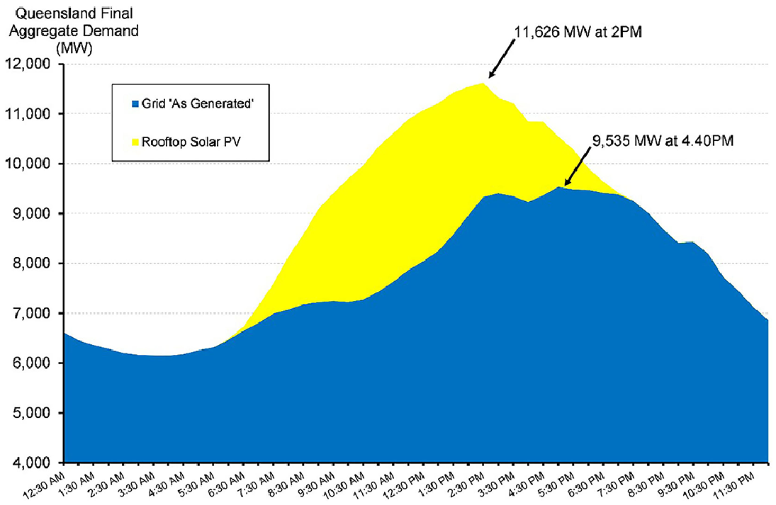
Aggregate final summer demand (grid-supplied & rooftop solar PV)—critical event summer day during February 2022.

During the spring months, and September in particular, ambient temperatures are mild with good solar irradiation, meaning household loads are moderate and rooftop solar output is strong. These conditions combine to produce a pronounced residual demand curve, excluding utility-scale solar PV, consistent with the duck curve (Figure 3). The requirement for more aggressive late afternoon-early evening ramping of plant is also apparent in Figure 3.

Figure 3.

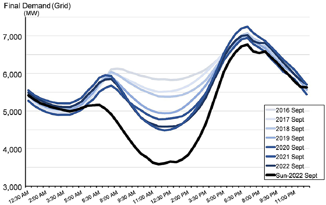
Queensland final (grid supplied) Demand- Avg Sept Day 2016–2022.

The most concerning aspect of Figure 3 is that the primary driver of the Queensland duck curve is primarily non-scheduled and therefore non-controllable rooftop solar PV—spread across ~800,000+ rooftops. Note in Figure 3 that daytime load has reduced significantly below the historic off-peak load point of 4am with the most acute impact occurring on Sundays. This minimum demand problem has led to a similar pattern of relative prices (Figure 4).

Figure 4.

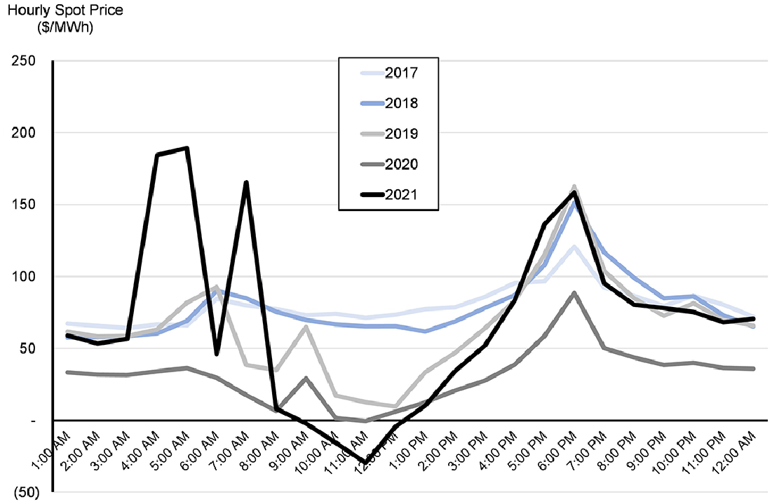
Queensland average spot prices (Sept/Oct) and negative price events.

Ironically, Queensland peak demand continues to rise whilst simultaneously minimum demand is declining (Figure 5, line series). As a result, the ramping of generators over a 4-hour period is increasing over time (Figure 5, bar series).

Figure 5.

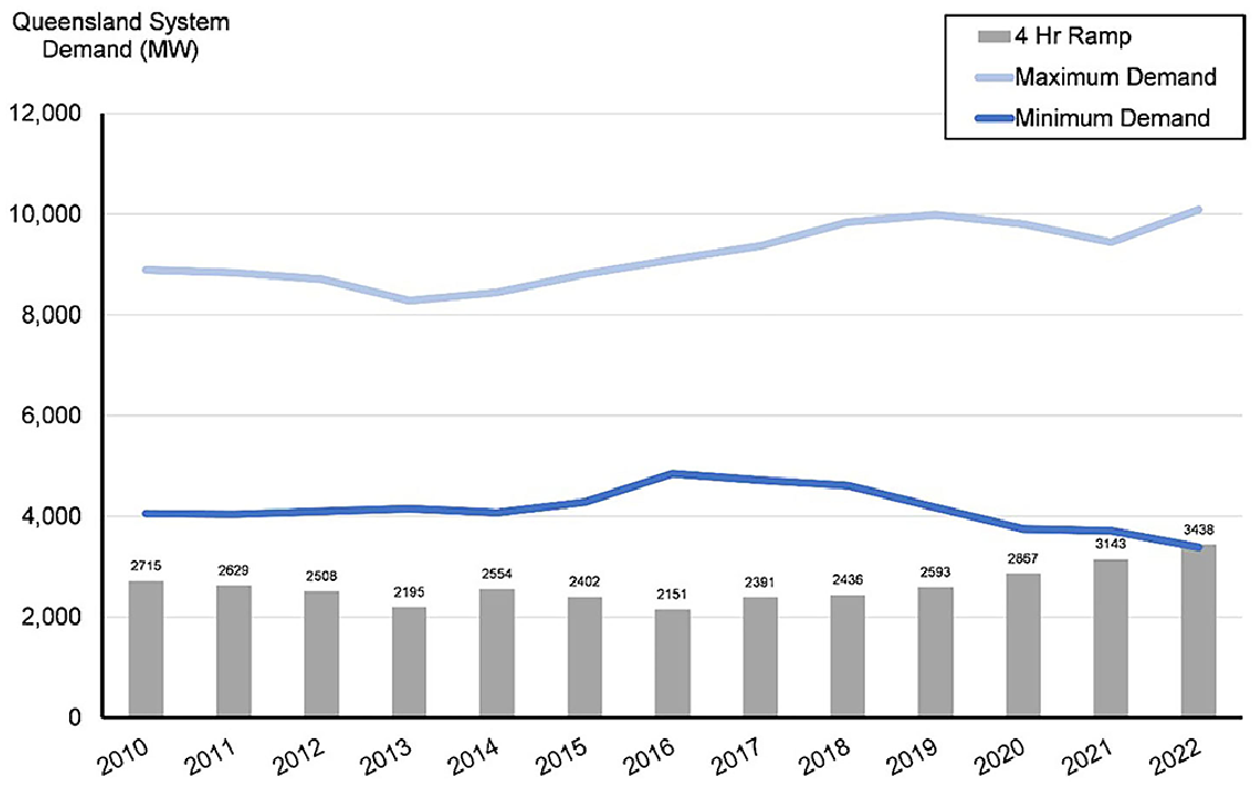
Queensland minimum and maximum demand, and 4-hour ramp.

The minimum load problem gives rise to two distinct issues for inflexible thermal plant. From an economic perspective, a rising incidence of negative prices is predictable and likely to drive financial distress of the marginal coal plant. From a technical perspective, the minimum load problem requires ever increasing interventions by the market operator.

With the benefit of hindsight, remediation appears straightforward. In the short run, install rooftop solar PV with field devices capable of curtailing output, and in the long run, exiting inflexible coal plant with entry dominated by flexible gas turbines and batteries (the latter helpfully adding to minimum loads when charging).

In Queensland, larger rooftop systems (10 kW+) are now required to couple field devices upon installation, which facilitates remote curtailment. But the political economy of applying such a policy to all new installations is surprisingly complex,⁹ and the transaction costs associated with retrofitting the existing 800,000+ rooftops or part thereof is prohibitive.

To summarize, the combination of inflexible thermal plant and rapidly declining minimum loads through rising rooftop solar PV will invariably impact the operation of the market. The non-continuous and unpredictable nature of minimum load events, “must run” requirements of inflexible coal plant and the (profitable) requirement of evening production duties by dispatchable plant means feasibility issues are likely to emerge. The nature of these problems may cause intractable dispatch issues within the mathematical programming methods employed to solve energy market equilibria in each trading interval.

3. Overview of ANEM Model and Data

Our “ANEM Model” is an agent-based structural model of a power system. The agents include demand- and supply-side participants as well as an Independent System Operator (ISO) who operates and clears the market. Nodes and transmission line network structures collectively constrain the behavior of all agents.

3.1. ANEM Model

The methodology underpinning the ANEM Model involves the operation of wholesale power markets by an ISO using Locational Marginal Pricing (LMP). ANEM is a modified and extended version of the American Agent-Based Modelling of Electricity Systems (AMES) model developed in (Sun and Tesfatsion 2007, 2010), and programmed in Java using Repast java toolkit (Repast 2023; Tesfatsion 2023).

A Direct Current Optimal Power Flow (DC OPF) algorithm is used to jointly determine optimal dispatch of generation plant, power flows on transmission branches and wholesale prices. The following unit commitment features are accommodated:

marginal generation costs;

capacity (MW) limits applied to both generators and transmission lines;

generator ramping constraints;

generator start-up costs; and

generator minimum stable operating levels.

Modeling methods used in this article on the minimum load problem are qualitatively similar to the Over-Constrained Optimisation Methods used by the Australian Energy Market Operator (AEMO) in the NEM’s dispatch algorithm (AEMO 2011, 2017). However, the underlying structure of our wholesale market model and the NEM’s dispatch algorithm are different and address quite different structural issues. In particular, our model has a more disaggregated network structure based on a nodal framework. Moreover, our model co-optimizes dispatch and both inter- and intra-regional transmission power flows (the market’s algorithm co-optimizes dispatch and inter-regional transmission branches).

3.2. DC OPF Solution Algorithm Used

Optimal dispatch, wholesale prices and power flows on transmission lines are determined in the ANEM model by a DC OPF algorithm developed in (Sun and Tesfatsion 2010). The (Mosek 2023)¹⁰ optimization software is used to solve the DC OPF problem.

The ANEM model solves the optimization for each half-hourly dispatch interval. The objective function minimizes real-power production levels $P_{G i}$ for all generators i = 1, . . . I, and voltage angles $δ_{k}$ for all transmission lines k = 2, . . . K subject to the three sets of constraints outlined below, relating to equality and inequality constraints. The optimization formally involves:

Objective function: Minimize generator-reported marginal costs and voltage angle differences

\sum_{i = 1}^{I} [A_{i} P_{G i} + B_{i} P_{G_{i}}^{2}] + π [\sum_{I_{m \in B R}} δ_{m}^{2} + \sum_{k m ϵ B R, k \geq 2} {[δ_{k} - δ_{m}]}^{2}],

where:

i = generator number

$P_{G i}$ = real power (MW) production level of generator i

k = transmission line number

$δ_{k}$ = voltage angle (in radians) at node k

subject to

Constraint 1: Nodal real power balance equality constraint

0 = P L o a d_{k} - P G e n_{k} + P N e t I n j e c t_{k}

where:

$P L o a d_{k} = \sum_{j ϵ J_{k}} P_{L_{j}}$ (i.e., aggregate power take-off at node k, e.g., demand)

$P G e n_{k} = \sum_{i ϵ I_{k}} P_{G_{i}}$ (i.e., aggregate power injection at node k, e.g., generation)

P N e t I n j e c t_{k} = \sum_{k m o r m k ϵ B R} F_{k m}

F_{k m} = B_{k m} [δ_{k} - δ_{m}]

(i.e., real power flows on branches connecting nodes “k” and “m”)

k = 1, . . . K

δ₁ ≡ 0, a normalization constraint.

Constraint 2: Transmission line real power inequality constraints

$F_{k m} \geq - F_{k m}^{U R},$ (lower bound constraint: reverse direction MW branch flow limit)

F_km ≤ F^UNkm (upper bound constraint: normal direction MW branch flow limit),

where:

$k m ϵ B R,$ transmission branch km is an admissible transmission branch interconnecting nodes k and m.

Constraint 3: Generator real-power production inequality constraints

$P_{G_{i}} \geq P_{G_{i}}^{L R},$ (lower bound constraint: lower half-hourly MW ramping limit)

P_Gi ≤ F^URki (upper bound constraint: upper half-hourly MW ramping limit),

where:

$P_{G_{i}}^{L R} \geq P_{G_{i}}^{L},$ (lower half-hourly ramping limit ≥ lower MW capacity limit)

P_URGi ≤ F^UGi (upper half-hourly ramping limit ≤ upper MW capacity limit),

i = 1, . . . I.

Note in the above discussion that “U” and “L” denote upper and lower limits, A_i and B_i are linear and quadratic cost coefficients from the generator’s variable cost function. $δ_{k}$ and $δ_{m}$ are the voltage angles at nodes “k” and “m.” Parameter π is a positive soft penalty weight on the sum of squared voltage angle differences. Variables $F_{k m}^{U N}$ and $F_{k m}^{U R}$ are the (positive) MW capacity limits associated with real power flows in the “normal” and “reverse” direction on each connected transmission branch $k m ϵ B R .$ Matrix $B_{k m}$ is negative susceptance matrix (Sun and Tesfatsion 2010).

The linear equality constraint refers to a nodal balance condition which requires that at each node, power take-off by the demand side equals power injection (by generators located at that node) and net power transfers from other nodes on “connected” transmission branches. For those interested in the transmission grid characteristics and the calculation of transmission losses, a summary appears in Appendix B.

3.3. Data: General Use of NEM Planning Assumptions

Our base model assumptions relating to ($/GJ) fuel cost, ($/MWh) Variable Operation and Maintenance (VOM) costs, ($/MW/year) Fixed Operation and Maintenance (FOM) costs, minimum and maximum MW capacities, emission intensity rates, auxiliary load rates and plant closures were sourced from the (AEMO 2022) biannual Integrated System Plan or “ISP assumptions and scenarios workbook v3.4 dated June 2022.”¹¹ Specifically, we follow the AEMO assumptions for the 2022 ISP associated with the “2030 step-change” scenario. Key ISP transmission augmentations accommodated in the modeling are listed in Appendix C. Further, while the model simulates the entire NEM, our model results focus specifically on the Queensland region—being of significant interest and the center of gravity vis-à-vis the minimum load problem.

To summarize the data, maximized dispatched MW capacities and energy output by technology type for Queensland and the entire NEM are listed in Tables 1 and 2. It should be recognized that the data listed in Tables 1 and 2 are for our base case (Scenario A), which is explained in detail in the next Section. For now, Scenario A contains coal generation and the largest number of intractable dispatch intervals of the modeled scenarios.¹²

Table 1.

Generating Capacity and Peak Demand for Queensland and the NEM.

Technology	NEM total	QLD total
Black coal	12,000	7,300
Brown coal	1,200	0
CCGT	3,700	1,500
OCGT	9,300	1,500
Wind	30,000	7,900
Solar (utility scale)	11,300	3,400
Conventional hydro	5,300	130
Pumped hydro	9,000	3,000
Batteries (utility)	6,700	1,800
Total	88,500	26,530
Rooftop solar PV	25,000	7,000
Peak demand	36,750	11,300

Table 2.

GWh by Technology for Queensland and the NEM.

Technology	NEM total	QLD total
Black coal	70,000	40,000
Brown coal	8,100	0
CCGT	13,000	6,000
OCGT	4,300	250
Wind	87,300	22,600
Solar (utility scale)	14,500	4,200
Conventional hydro	1,500	0
Pumped hydro	3,800	500
Batteries (utility)	1,500	250
Total generation	204,000	73,800
Rooftop solar PV	49,000	15,000
Energy demand (operational)	184,000	55,600

From inspection of Table 1 it is apparent that Queensland has a significant portfolio of coal and Combined Cycle Gas Turbine (CCGT) assets within the NEM. Both technologies have non-zero minimum stable operating levels which drive feasibility issues within the wholesale electricity market under “low load, high renewables” conditions.

Queensland also has a significant existing Open Cycle Gas Turbines (OCGT) fleet that is well suited to meeting peak demand events. Forecast levels of wind and solar capacity equate to 7,900 MW and 3,400 MW, respectively. Queensland is also anticipating significant (2,000 MW) pumped-hydro and utility-scale battery capacities located in Northern and Southern Queensland. The forecast of rooftop solar PV for 2030 in Queensland is 7,000 MW, up from the current 6,000 MW.¹³

Finally, the maximum half-hourly peak demand for Queensland in the step-change scenario for 2030 is 11,300 MW. This compares to Queensland’s existing peak of 11,000 MW and the (diversified instantaneous) NEM-wide peak of 36,750 MW.

In Table 2, base case results from our model vis-à-vis energy generated by technology type is listed for Queensland and the entire NEM. By way of brief background, NEM coal plant marginal running costs range from $10 to $60/MWh while CCGT and OCGT plant are typically leveraged to ~$9/GJ gas costs, meaning marginal running costs of ~$65/MWh and ~$100/MWh, respectively.

From inspection of Table 2 it is evident that significant energy is produced by coal and CCGT generation assets in Queensland. Queensland grid-supplied energy demand of 55,600 GWh associated with the 2030 step-change scenario can be compared to the equivalent NEM-wide energy demand of 184,000 GWh. Note this demand is a net concept associated with centralized operational demand.

Energy generated in Queensland by rooftop solar is projected at 15,000 GWh, the third largest contributor after coal and wind generation. Interestingly, the sum of rooftop and utility-scale solar in Queensland equates to 19,200 GWh, thus resembling the contribution from wind generation at 22,600 GWh.

It should be noted that the last row in Table 2 provides operational energy demand that was produced by the market operator (AEMO) as part of their Integrated System Planning process. This demand concept, however, excludes any additional demand determined from the modeling to support:

Storage loads from pumped hydro and utility-scale batteries.

Transmission losses that are allocated as additional nodal demands.

Moreover, significant export of energy from Queensland to New South Wales arose, that is some of the generation in the third column of Table 2 would, in fact, end up serving New South Wales demand. It is for these reasons that total generation (row 11) exceeds operational energy demand (row 14) in Table 2.

Operational demand is calculated by AEMO as a net demand concept equating to gross demand less behind the meter consumer economic resources including rooftop solar and household-level batteries. From the perspective of estimating residential consumption, the latter components include estimations of (AEMO 2023):

Impact of electrical appliance uptake;

Impact of the solar PV rebound effects (Beppler, Matisoff and Oliver 2023; Boccard and Goutier 2021; Deng and Newton 2017; Frondel et al. 2023; Mahdavi Mazdeh 2023; Qiu, Kahn and King 2019)¹⁴;

Impact of climate change;

Impact of consumer behavioral response to retail price changes;

Impact of energy efficiency savings; and

As noted above, the impacts of Consumer Energy Resources comprising rooftop solar PV, household batteries and electric vehicles.

In relation to the solar rebound effects, Mahdavi Mazdeh (2023) found morning and evening peaks were present in PV rebounds in all considered regions in Australia’s NEM, although the morning peak tended to shift to mid-morning when moving from summer to winter. Importantly, these time periods do not closely align with time periods experiencing the greatest duck curve impacts which instead arise during late morning and into the early afternoon.

The projected capacity of residential batteries is also expected to remain below that of rooftop solar PV out to 2030, representing 26.1 percent of rooftop solar PV in terms of battery discharging capacity and increasing to 30.7 percent when converting to effective battery charging capacity assuming a round-trip efficiency of 85 percent that was used in the 2022 ISP (AEMO 2022). Out to 2030, these capacities fall well short of what would be needed to significantly ameliorate duck curve impacts through behind the meter battery charging operations during time periods aligned to the incidence of the most severe duck curve impacts.

Therefore, many distributed consumer resources such as uptake of rooftop PV, electric vehicles and battery storage as well as the solar rebound effects were explicitly estimated or modeled by AEMO when compiling residential demand and, in the case of distributed consumer resources, were subtracted from gross demand to derive the operational demand concept utilized in the modeling.

3.4. Modeling Pumped Hydro and Batteries

The energy contribution of pumped hydro and utility-scale batteries are moderate at 500 GWh and 250 GWh, respectively (Table 2). This outcome reflects the relatively large operational coal generation fleet in Queensland under the base case scenario, which crowds-out opportunities for pumped-hydro and batteries.

The round-trip efficiency for new pumped hydro and batteries was assumed to be 0.76 and 0.84 percent respectively, broadly matching assumptions employed in the ISP.¹⁵ Where available, round-trip efficiencies were derived from actual data for operational pumped hydro plant. The round-trip efficiencies assumed means that 658 GWh of storage energy for pumping would have been expended in the case of Queensland pumped hydro dispatch of 500 GWh and around 298 GWh of energy would have been expended in charging Queensland utility-scale batteries for its dispatch of 250 GWh under Scenario A, for example.

Axiomatically, coal plant exit changes these results considerably. In the case where Queensland’s marginal coal plant is closed, Queensland pumped hydro dispatched 1,590 GWh of energy at a calculated round-trip efficiency of 0.7654 and energy expended for pump actions of 2,080 GWh. Note also that the round-trip efficiency is closer to the assumed rate of 0.76. Pumped hydro output rises as further coal units are closed.

Pumped-hydro and battery technologies undertake a nuanced role in the market given their ability to absorb otherwise “excess output” from intermittent solar PV and wind generation. In the NEM, the typical diurnal cycle of wind is biased to the night-time and solar PV has a day-time bias.

In the modeling, pumping or charging loads of both pumped-hydro and batteries were targeted toward periods where the underlying variable renewable resources were sufficient to supply both underlying aggregate demand as well as additional demand created through pumping or charging loads.¹⁶ Pumping/charging of these resources also facilitates increased power from wind and solar generation plant and reduces curtailment or “spill.”

In practical terms, this generally means that pumping loads occur during the periods:

11 pm to 5.30 am (when excess wind exists) and

10 am to 3.30 pm (when excess solar exists).

For batteries, the equivalent charging periods typically arising are:

Midnight to 4 am and

10 am to 3 pm.

To be clear, pumping and charging loads would typically not occur over morning or evening peaks and in the period leading toward midnight because the diurnal cycle of wind generation is weaker.

In the model, pumped-hydro and battery supply offers generally fall between coal and open cycle gas plant, targeting a balancing roll but with a competitive advantage conferred relative to peak load OCGT technologies. This strategy has two facets: (1) it maximises the roll that storage technologies can contribute to system balancing and (2) determining the minimum sizing of gas generation capacity that might still be needed for system balancing.

4. Salient Features of Minimum Load Events

Our modeling seeks to identify the frequency of binding minimum load events.¹⁷ During these episodes, the dispatch algorithm becomes intractable because of extremely low grid-supplied loads and a prevalence of inflexible generation plant seeking to dispatch at their “must run” minimum stable loads when a clear oversupply exists. In these circumstances, the optimization algorithm has to optimally change the default set of constraints producing episodes of intractable dispatch in order to secure feasible and optimal solutions needed for stable dispatch outcomes. Technically, this process is termed “feasibility repair” and can help identify the sources of intractability arising under the default set of constraints. Once identified, we proceed by examining increasing rates of coal plant closures to identify what level is technically, and economically, inevitable given the ongoing surge in new VRE capacity.

Queensland’s coal fleet currently comprises 8,100 MW of generating plant. Between now and 2030, our base case assumes the closure of only one coal plant 700 MW (i.e., Callide B power station). The coal fleet in New South Wales currently comprises about 10,350 MW and our base case for 2030 assumes ~5,000 MW of coal plant closures (i.e., Liddell and Eraring power stations).

Our base case commences as the highest level of coal capacity in service, at 13,200 MW in aggregate (nb. including 1,200 MW of brown coal in the Victorian region). Our studies then focus on exiting two marginal coal plants in Queensland and New South Wales—the 1,600 MW Gladstone and 1,320 MW Vales Point power stations, respectively.

When our model runs for the 2030 year at 30-minute resolution under the base case scenario, we find a total of 711 minimum load intervals. That is, the model experiences 711 intractable half-hourly dispatch intervals in the base case. The timing of the incidence of dispatch intervals (by month) from the model is presented in Figure 6.

Figure 6.

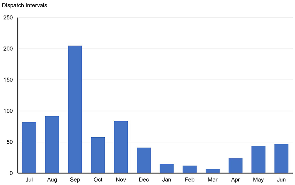
Incidence of minimum loads by month (2030).

Examination of Figure 6 reveals that minimum loads primarily occur during spring (September 205 intervals, November 84 intervals) and winter (August 92 intervals, July 82 intervals). There are notably more intervals over the period July to November. The lowest values occur during the NEM’s peak demand quarter, Jan-Mar. Finally, it is worth noting that dispatch intervals associated with minimum load events occurred across all months.

Figure 7 plots the incidence of minimum load intervals by time-of-day. Binding minimum loads are concentrated during daylight hours, centered either side of 12:00pm with no incidences during overnight periods.

Figure 7.

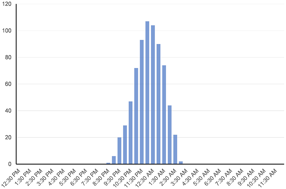
Minimum load events by time of day.

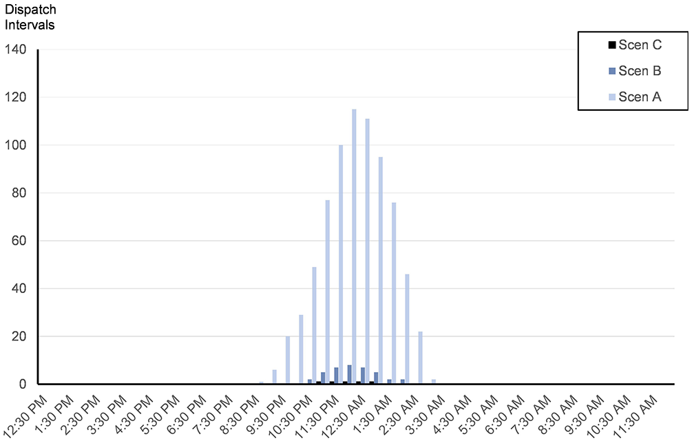
In order to gage the incidence of minimum load intervals vis-à-vis operating coal plant capacity, we compare our base case (labeled Scenario A, dark blue bars) with a scenario in which the two marginal coal plants in Queensland (1,600 MW Gladstone) and New South Wales (1,320 MW Vales Point) exit the market (labeled Scenario B, light blue bars). Output from these coal generators is replaced by renewable and gas generation, and in order to ensure reliability criteria is met in Queensland following the loss of 1,600 MW, an additional 800 MW of dispatchable plant (viz. gas turbines, batteries, pumped hydro) is commissioned. Average prices increase from $35/MWh (Scenario A, which exhibits very material merit order effects) to $67/MWh (Scenario B). These prices shadow supply offer prices of coal plant in Scenario A, increasing to the lower bounds supply offers associated with dispatchable capacity from pumped-hydro, batteries and gas turbines in Scenario B. Scenario C (black bars) deducts an additional 350 MW coal unit in Queensland (from the next marginal coal plant, Stanwell power station).¹⁸ Results are presented in Figure 8.

Figure 8.

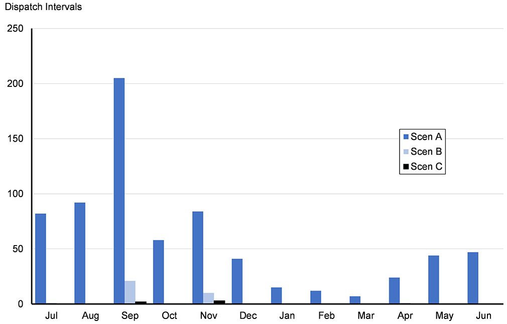
Total incidence of minimum loads by month and scenario.

The first major outcome that we identify in Figure 8 is a very material reduction in minimum load half-hourly dispatch intervals in Scenario B through the exit of the 1,600 MW Gladstone and 1,320 MW Vales Point coal plants. The closure of a 350 MW unit in Scenario C further reduces the incidences of intractable dispatch which appear in September and November, suggesting transient unit de-commitment may be sufficient. To summarize Figure 8:

The total number of minimum load half-hour intervals in Scenario C = 5, (3 intervals in November and 2 in September)

The total number of minimum load half-hour intervals in Scenario B = 33, (21 intervals in September and 10 in November)

The total number of minimum load half-hour intervals in Scenario A = 711

Figure 9 plots the incidence of minimum loads by half-hourly dispatch interval for each Scenario. Consistent with the results from Figure 7, minimum loads were centered either side 12.00pm, with particular concentration around the 11 am to 1 pm time-period.

Figure 9.

Total incidence of minimum load intervals.

It is also emphasized that the results in Figure 9 (and in Figure 8), indicate that there were no minimum load events in Scenarios B and C in any other months besides September and November.

From these model results we may conclude the following:

The incidence of minimum load events was directly linked to an oversupply of inflexible coal plant. Scenario A included the highest level of operational coal plant capacity and had the highest incidence of minimum load events. This tapered off with coal plant closures.

The greatest extent of minimum load events occurs in the months of July, August, September and November. October exhibits a curiously lower incidence likely related to increased maintenance activity during that month.¹⁹

The lowest number of minimum load events occurs over summer when household air conditioning loads are at their peak.

Minimum load events are centered over the half hour 12pm. This links feasibility issues with episodes of the minimum load problem.

All minimum load events occurred during daytime—none emerged overnight or during morning and evening peak periods.

5. The Anatomy of Constraint Violations

Recall that in our model, minimum load events require constraint relaxations to secure primal and dual feasible solutions that are not forthcoming under original constraint settings. In Section 4, we observed feasible repair intervals tended to be concentrated around 12:00pm. We also suggested in Section 4 that the nature of constraint violations, given those patterns, were likely to be produced by emergent duck curve effects where rooftop solar naturally diminishes grid-supplied demand, posing problems for solving the wholesale market when inflexible coal generation plant dominates the (dispatchable) aggregate supply function.

Coal plant non-zero minimum stable loads combine to ensure centralized demand is frequently insufficient to satisfy the minimum “must-run” requirements of the available coal fleet during “minimum load intervals.” In practice, the early warning signs of this will be a gradual increase in the frequency and intensity of negative price events. These events will simultaneously begin to erode the net profit margins and quantities dispatched of inflexible thermal plant. This is well documented in the energy economics literature and comprises a combination of price impression effects (Edenhofer et al. 2013; Hirth, Ueckerdt and Edenhofer 2016; Mills, Wiser and Lawrence 2012; Nicolosi 2012), stochastic production effects (Johnson and Oliver 2019; Simshauser 2020), and utilization effects (Hirth 2013; Höschle et al. 2017; Simshauser 2018).

Conversely, operational flexibility is likely to become an increasingly valuable plant characteristic. Another potentially valuable characteristic may be higher MW transfer capacities on transmission branches to enhance the ability to shift power around the transmission network by enhancing its geographic reach, and diversity of minimum loads.

Accordingly, we now turn our modeling efforts to examining the extent to which these factors emerge within constraint violations. Specifically, we investigate the extent that minimum load events arise as a result of (1) non-zero minimum stable (i.e., must-run) operating levels of coal and CCGT plant and (2) normal and reverse direction MW transfer capacity limits on transmission lines. On (2), particular attention will be given to investigating the presence of network congestion across the Queensland to New South Wales Interconnector—to clarify whether it is possible to “export your way out of the problem”—via accessing inter-regional load diversity.

5.1. Non-zero Minimum Stable Load Constraint Violations

The catalog of constraint violations for all minimum load events across coal and CCGT plant are illustrated in Figure 10. Note in this context, constraint violation would mean that a lower constraint was imposed compared to the original constraint setting associated with primal infeasibility. As such, this process would mimic key aspects of greater operational flexibility: (1) the ability to shut-down quickly and (2) the ability to operate at lower part-load capacities.

Figure 10.

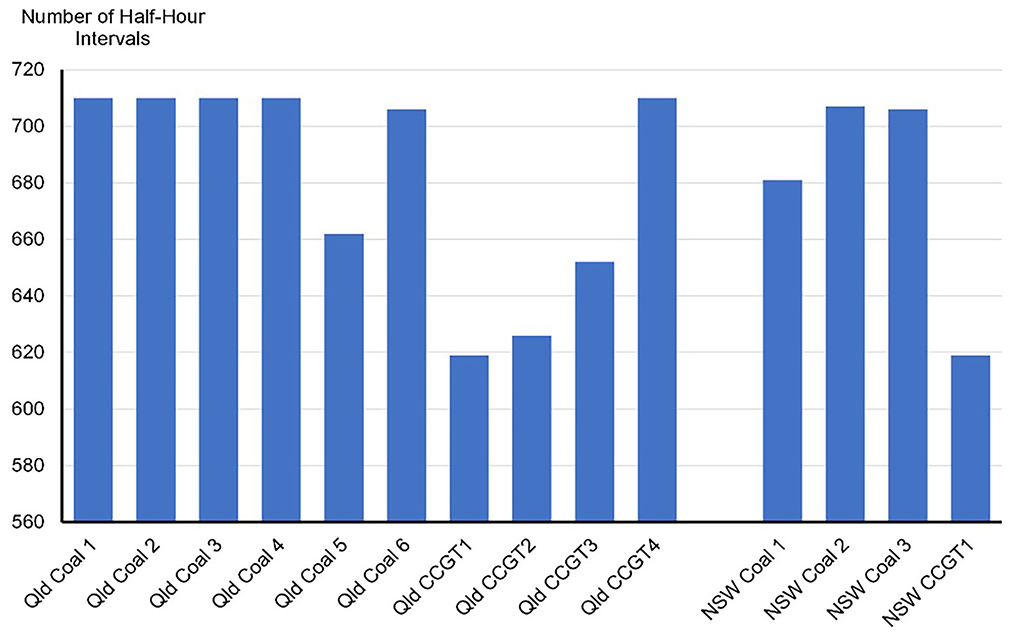
Constraint violations for coal and CCGT by power station (half-hour count).

The data was collated by assessing if the original constraint settings of the plant listed in Figure 10 were violated during a minimum load event. The results for each plant was collated across the 711 minimum load intervals associated with Scenario A.

The first point to note from Figure 10 is the large number of affected plant located in Queensland compared to NSW. But ultimately, all black coal and CCGT plant in both regions are affected. Second, CCGT units were principally aligned to supplying power during the morning and evening peak periods, thus had lesser exposures to minimum load events. Finally, there is some variability across, and within, coal plants. For example, Queensland Coal Plant #5 experienced considerably less constraints than the other coal plants. And while not visible through inspection of Figure 10, Queensland Coal Plant #1 comprises 4 × 350 MW units, and of these, one unit experienced only 200 half-hour intervals of constraints whereas the remaining 3 units were impacted in all 711 dispatch intervals. These variations reflect planned overhauls or forced outages had coincided with elevated episodes of minimum load (i.e., primarily during the spring maintenance season).

To summarize, we can confirm the source of the problem is the combination of low grid-supplied demand and the presence of inflexible thermal plant unable to lower their minimum stable loads.

5.2. Queensland to New South Wales Interconnector

One logical line of inquiry is to test whether a state like Queensland can export its way out of trouble during minimum load events. This requires an examination of underlying demand conditions as well as transmission network properties and flows during minimum load events.

Figure 11 presents a scatter plot of operational demand in Queensland (x-axis) and New South Wales (y-axis) during feasible repair intervals under Scenario A. Note the tighter demand range prevailing for Queensland relative to New South Wales, with Queensland low loads falling between 1,720 and 3,600 MW and New South Wales falling between 1,720 and 9,400 MW (noting state peak demands are 11,300 MW and 14,600 MW, respectively). Examination of Figure 11 reveals sizable concentrations of scatter points encompassing coincident minimum loads, viz. below 4,000 MW in New South Wales and below 3,600 MW in Queensland.

Figure 11.

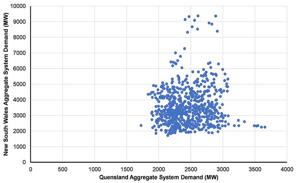
QLD and NSW system demand during QLD minimum load events.

The other crucial factor that may impact Queensland’s ability to export power to the adjacent region is whether the interconnector to New South Wales experiences congestion during minimum load events. Figure 12 depicts power transfers on the main Queensland to New South Wales Interconnector, which is currently a double circuit 330 kV transmission line and an assumed second circuit,²⁰ meaning a southerly flow limit of 1,700 MW. Figure 12 tends to suggest the “exporting your way out” of the minimum load problem is not viable—exports across the interconnector peak at 1,200 MW, well below the 1,700 MW limit. Evidently, the minimum load problem is a largely simultaneous matter affecting both regions.

Figure 12.

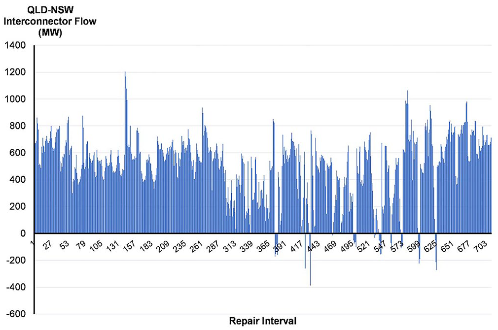
Interconnector flows during QLD minimum load events.

6. Conclusions and Policy Considerations

In this article, we examined a new frontier emerging in the NEM’s Queensland region, the minimum load problem. The origins of the minimum load problem are the hollowing out of daytime grid-supplied load (cf. aggregate final demand) during high solar irradiation and mild weather conditions combined with an oversupply of inflexible coal plant. The situation in Queensland differs in subtle ways from other variants of the so-called “duck curve” effect in that the source of the problem comes principally from non-scheduled (small-scale) rooftop solar PV, large parts of which are uncontrolled and therefore non-curtailable. Production inflexibility of legacy coal generation plant forms the other limb of this emerging problem.

Our results suggest ~700 half-hour intervals per annum in which the minimum load problem becomes binding. Binding minimum loads occurred throughout the year but were heightened in the winter and spring months of July, August, September and November. The minimum load problem was centered around 12 noon. The interconnector to the adjacent region of New South Wales could not be expanded to “export your way out of the problem.”

At a strategic level, if a feasible solution to the wholesale electricity market cannot be attained then spot price and generation dispatch schedules cannot be posted. In these circumstances and without feasibility repair, the wholesale electricity market would experience gross malfunction—in essence, the market would become broken.

The troubling aspect of our modeling, which may understate the nature of the problem, is that our assumptions book included a new 2,000 MW pumped hydro project that is currently unlikely to enter into service prior to 2030. In practical terms, this means the development of a fleet of new entrant, flexible, dispatchable plant to replace aging inflexible legacy coal plant is rather urgent.

What can other potentially solar-rich jurisdictions with inflexible thermal generation fleets learn from Queensland? The first and most obvious policy lesson vis-à-vis the roll-out of rooftop solar PV in large numbers is to ensure appropriate field devices are included during initial installation to allow central coordination (i.e., curtailment) if required for system security purposes. The transaction costs of retrofitting make this quite important.

Second, more thought is required vis-à-vis exit and entry. When energy markets were being designed, and in particular Australia’s National Electricity Market during the early-1990s, the problem being solved was oversupply, prices set above efficient levels, state ownership and underperforming generators in an environment of solid demand growth. Market design therefore focused on productive and allocative efficiency, and the dynamic efficiency of entry (see Bublitz et al. 2019).

To the best of our knowledge, little policy thought was given to exit. Discussions of plant exit while governments were privatizing their power assets would send mixed signals to potential buyers. Yet exit is now an important issue and the NEM’s recent history of coal plant closures has been anything but smooth (see Dodd and Nelson 2019; Nelson, Nolan and Gilmore 2022; Nelson, Orton and Chappel 2018; Rai and Nelson 2020; Simshauser and Gilmore 2022)

Our analysis tends to suggest that the exit of inflexible coal plant in the presence of sharply rising levels of intermittent renewables must be carefully orchestrated, particularly given the proliferation of a vast fleet of non-scheduled (and therefore uncontrollable) rooftop solar PV.

Sudden exit requires the rapid entry of flexible plant, including batteries, gas turbines and pumped hydro plant absent a large, pliable and highly elastic demand-side response. The demand-side has long been the underperforming element of the wave of energy market reforms commencing in the 1990s (see Batlle and Pérez-Arriaga 2008; Bublitz et al. 2019; Cramton and Stoft 2008; Finon and Pignon 2008; Roques 2008). Queensland has witnessed a decade-long solar revolution along with deteriorating midday prices (per Figure 4) and we are not aware of any material change in power system loads in response. What we have observed is the trends and patterns outlined in Figures 3 to 5, namely falling minimum loads, ongoing rises in peak demand, an ever-growing ramp rate requirement, an aging coal fleet (with increasing outage rates), and a sharp rise in the incidence of negative prices which does not bode well for inflexible plant.

Supplemental Material

sj-pdf-1-enj-10.1177_01956574241283732 – Supplemental material for Rooftop Solar PV, Coal Plant Inflexibility and the Minimum Load Problem

Supplemental material, sj-pdf-1-enj-10.1177_01956574241283732 for Rooftop Solar PV, Coal Plant Inflexibility and the Minimum Load Problem by Paul Simshauser and Phillip Wild in The Energy Journal

Footnotes

Appendix A

Appendix B. Modeling Transmission Losses

Transmission losses associated with power flows on transmission branches were determined by the DC OPF solution and were calculated for each transmission branch using the methodology outlined in Section 5 of (AEMO 2012). That is, transmission losses are calculated by multiplying the square of the power flow on each transmission branch determined by the DC OPF solution by that branch’s line resistance and a factor of proportionality associated with conversion of line current to real power in a three-phase electrical system. These losses are allocated as fictitious nodal demand to the receiving end node—that is, to the node that the power is flowing on the transmission branch toward. The key impact of this operation is to ensure that enough power is generated by generators to both cover transmission losses as well as meeting native demand offtake at each node.

Appendix C. ANEM Model Inter-state Interconnector Details

The transmission grid utilized in the ANEM model is an AC grid modeled as a balanced three-phase network defined according to the design features outlined in (Sun and Tesfatsion 2010). The following inter-state interconnectors link the NEM’s five zones:

In addition, the following ISP actionable transmission augmentation relevant to our analysis included in the modeling were:

Table of Acronyms

$/GJ Dollars per Gigajoule

$/KW Dollars per Kilowatt

c/KWh Cents per Kilowatt hour

$/MWh Dollars per Megawatt hour

$/MW/year Dollars per Megawatt per Year

AEMO Australian Energy Market Operator

AMES American Agent-Based Modelling of Electricity Systems Model

ANEM Wholesale Electricity Market Model of the NEM

BESS Battery Energy Storage System

CAISO California Independent System Operator

CCGT Combined Cycle Gas Turbine

DC OPF Direct Current Optimal Power Flow

EV Electric Vehicle

FOM Fixed Operation and Maintenance Costs

GJ Gigajoule

GWh Gigawatt hour

ISO Independent System Operator

ISP AEMO’s Integrated System Plan

kV Kilovolts

KW Kilowatts

LMP Locational Marginal Price

MOSEK Mosek Aps: Optimisation Software Package

MW Megawatt

NEM National Electricity Market

NSW New South Wales (Australian State)

OCGT Open Cycle Gas Turbine

OCT October

PHES Pump Hydro Energy Storage

PV Photovoltaics

QLD Queensland (Australian State)

QNI Large AC interconnector linking QLD and NSW

REPAST Agent-Based Modelling Simulation Software Platform

REZ Renewable Energy Zone

SA South Australia (Australian State)

SEPT September

TAS Tasmania (Australian State)

VIC Victoria (Australian State)

VOM Variable Operation and Maintenance Costs

VRE Variable Renewable Energy

Declaration of Conflicting Interests

The author(s) declared no potential conflicts of interest with respect to the research, authorship, and/or publication of this article.

Funding

The author(s) received no financial support for the research, authorship, and/or publication of this article.

Supplemental Material

Supplemental material for this article is available online at DOI: https://doi.org/10.25904/1912/5530 or alternatively at

Notes

References

AEMO. 2011. “Over-Constrained Dispatch Rerun Process Document.” https://www.aemo.com.au/-/media/Files/Electricity/NEM/Security_and_Reliability/Congestion-Information/2016/Over-Constrained-Dispatch-Rerun-Process.pdf.

AEMO. 2012. “Treatment of Loss Factors in the National Electricity Market.” https://www.aemo.com.au/-/media/Files/Electricity/NEM/Security_and_Reliability/Loss_Factors_and_Regional_Boundaries/2016/Treatment_of_Loss_Factors_in_the_NEM.pdf.

AEMO. 2017. “Constraint Relaxation Procedure.” https://aemo.com.au/media/files/electricity/nem/security_and_reliability/congestion-information/2016/constraint-relaxation-procedure.pdf.

AEMO. 2022. “2022 Integrated System Plan June 2022 for the National Electricity Market.” https://aemo.com.au/-/media/files/major-publications/isp/2022/2022-documents/2022-integrated-system-plan-isp.pdf?la=en.

AEMO. 2023. “Forecasting Approach –Electricity Demand Forecasting Methodology August 2023: Applied in Developing the 2023 Electricity Statement of Opportunities Forecast.” https://aemo.com.au/-/media/files/electricity/nem/planning_and_forecasting/nem_esoo/2023/forecasting-approach_electricity-demand-forecasting-methodology_final.pdf.

Ahmad

S. S.

Al-Ismail

F. S.

Almehizia

A. A.

Khalid

2020. “Model Predictive Control Approach for Optimal Power Dispatch and Duck Curve Handling Under High Photovoltaic Power Penetration.” IEEE Access 8: 186840–50. doi:10.1109/ACCESS.2020.3030100.

Badrzadeh

Emin

Goyal

Grogan

Haddadi

Halley

Louis

2021. “System Strength.” CIGRE Science & Engineering 20: 5–26.

Batlle

Pérez-Arriaga

I. J.

2008. “Design Criteria for Implementing a Capacity Mechanism in Deregulated Electricity Markets.” Utilities Policy 16: 184–93. doi:10.1016/j.jup.2007.10.004

Beppler

R. C.

Matisoff

D. C.

Oliver

M. E.

2023. “Electricity Consumption Changes Following Solar Adoption: Testing for a Solar Rebound.” Economic Inquiry 61: 58–81. doi:10.1111/ecin.13031.

10.

Berrie

1967. “The Economics of System Planning in Bulk Electricity Supply.” Electrical Review 22: 425–8.

11.

Boccard

Goutier

2021. “Solar Rebound: The Unintended Consequences of Subsidies.” Energy Economics 100: 105334. doi:10.1016/j.eneco.2021.105334.

12.

Boiteux

1949. “La tarification des demandes en pointe: Application de la theorie de la vente au cout marginal in Revue. Generale de l’Electricite. Translated by: Izzard, H. (1960).” Journal of Business 33: 157–80. https://www.jstor.org/stable/2351015.

13.

Bonbright

Danielsen

Kamerschen

1988. Principles of Public Utility Rates. 2nd ed. Arlington, TX: Public Utilities Reports Inc.

14.

Bublitz

Keles

Zimmermann

Fraunholz

Fichtner

2019. “A Survey on Electricity Market Design: Insights From Theory and Real-World Implementations of Capacity Remuneration Mechanisms.” Energy Economics 80: 1059–78. doi:10.1016/j.eneco.2019.01.030.

15.

Bunn

Yusupov

2015. “The Progressive Inefficiency of Replacing Renewable Obligation Certificates With Contracts-for-Differences in the UK Electricity Market.” Energy Policy 82: 298–309. doi:10.1016/j.enpol.2015.01.002.

16.

Bye

1929. “Composite Demand and Joint Supply in Relation to Public Utility Rates.” The Quarterly Journal of Economics 44: 40–62. doi:10.2307/1885440.

17.

CAISO. 2013. “What the Duck Curve Tells Us About Managing a Green Grid.” CAISO Publication. https://www.caiso.com/Documents/FlexibleResourcesHelpRenewables_FastFacts.pdf. Accessed March 8, 2023.

18.

Calabrese

1947. “Generating Reserve Capacity Determined by the Probability Method.” Transactions of the American Institute of Electrical Engineers 66: 1439–50. doi:10.1109/T-AIEE.1947.5059596.

19.

Cludius

Forrest

MacGill

2014. “Distributional Effects of the Australian Renewable Energy Target (RET) Through Wholesale and Retail Electricity Price Impacts.” Energy Policy 71: 40–51. doi:10.1016/j.enpol.2014.04.008.

20.

Cramton

Stoft

2008. “Forward Reliability Markets: Less Risk, Less Market Power, More Efficiency.” Utilities Policy 16: 194–201. doi:10.1016/j.jup.2008.01.007.

21.

Crew

M. A.

Kleindorfer

P. R.

1976. “Peak Load Pricing With a Diverse Technology.” Bell Journal of Economics 7: 207–31. doi:10.2307/3003197.

22.

Deng

Newton

2017. “Assessing the Impact of Solar PV on Domestic Electricity Consumption: Exploring the Prospect of Rebound Effects.” Energy Policy 110: 313–24. doi:10.1016/j.enpol.2017.08.035.

23.

Denholm

O’Connell

Brinkman

Jorgenson

2015. “Overgeneration From Solar Energy in California: A Field Guide to the Duck Chart.” NREL TP-6A20-65023. National Renewable Energy Lab, Golden, CO.

24.

Dodd

Nelson

2019. “Trials and Tribulations of Market Responses to Climate Change: Insight Through the Transformation of the Australian Electricity Market.” Australian Journal of Management 44: 614–31. doi:10.1177/0312896219874096.

25.

Edenhofer

Hirth

Knopf

Pahle

Schlomer

Schmid

Ueckerdt

2013. “On the Economics of Renewable Energy Sources.” Energy Economics 40: S12–23. doi:10.1016/j.eneco.2013.09.015.

26.

Felder

2011. “Examining Electricity Price Suppression Due to Renewable Investments.” Electricity Journal 24: 34–46. doi:10.1016/j.tej.2011.04.001.

27.

Finon

Pignon

2008. “Capacity Mechanisms in Imperfect Electricity Markets.” Utilities Policy 16: 141–2. doi:10.1016/j.jup.2008.01.006.

28.

Forrest

MacGill

2013. “Assessing the Impact of Wind Generation on Wholesale Prices and Generator Dispatch in the Australian National Electricity Market.” Energy Policy 59: 120–32. doi:10.1016/j.enpol.2013.02.026.

29.

Frondel

M. F.

Kaestner

Sommer

Vance

2023. “Photovoltaics and the Solar Rebound: Evidence From Germany.” Land Economics 99: 265–82. doi:10.3368/le.070621-0077R1.

30.

Greene

1896. “A Method of Calculating the Cost of Furnishing Electric Current and a Way of Selling It.” The Electrical World 23: 222–8. Republished in: “The development of scientific rates for electricity supply.” Reprints of selected original rate papers. Detroit: The Edison Illuminating Company of Detroit, 1915, Detroit.

31.

Hardt

Premm

Mayer

Mosallat

Goyal

2021. “Practical Experience With Mitigation of Sub-Synchronous Control Interaction in Power Systems With Low System Strength.” CIGRE Science & Engineering 21: 5–13.

32.

Hirth

2013. “The Market Value of Variable Renewables. The Effect of Solar Wind Power Variability on Their Relative Price.” Energy Economics 38: 218–36. doi:10.1016/j.eneco.2013.02.004.

33.

Hirth

Ueckerdt

Edenhofer

2016. “Why Wind is Not Coal: On the Economics of Electricity Generation.” The Energy Journal 37: 1–27. doi:10.5547/01956574.37.3.lhir.

34.

Hopkinson

1892. “On the Cost of Electric Supply.” Transactions of the Junior Engineering Society 3: 1–14. Republished in: The development of scientific rates for electricity supply. Reprints of selected original rate papers. Detroit: The Edison Illuminating Company of Detroit, 1915, Detroit.

35.

Höschle

De Jonghe

Le Cadre

Belmans

2017. “Electricity Markets for Energy, Flexibility and Availability — Impact of Capacity Mechanisms on the Remuneration of Generation Technologies.” Energy Economics 66: 372–83. doi:10.1016/j.eneco.2017.06.024.

36.

Hotelling

1938. “The General Welfare in Relation to Problems of Taxation and of Railway and Utility Rates.” Econometrica 6: 242–69. doi:10.2307/1907054.

37.

Houthakker

H. S.

1951. “Electricity Tariffs in Theory and Practice.” The Economic Journal 61: 1–25. doi:10.2307/2226608.

38.

Johnson

E. P.

Oliver

M. E.

2019. “Renewable Generation Capacity and Wholesale Electricity Price Variance.” The Energy Journal 40: 143–68. doi:10.5547/01956574.40.5.ejoh.

39.

Joskow

P. L.

1976. “Contributions to the Theory of Marginal Cost Pricing.” The Bell Journal of Economics 7: 197–206. doi:10.2307/3003196.

40.

Lewis

1941. “The Two-Part Tariff.” Economica 8: 249–70. doi:10.2307/2549332.

41.

Mahdavi Mazdeh

2023. “Solar PV Rebound Effect on Regional Demand.” IEEE Sustainable Power and Energy Conference 2022, Perth, Australia, 1–5. IEEE. doi:10.1109/iSPEC54162.2022.10032991.

42.

Martin

Diesendorf

1983. “The Economics of Large-Scale Wind Power in the UK: A Model of an Optimally Mixed CEGB Electricity Grid.” Energy Policy 11: 259–66. doi:10.1016/0301-4215(83)90082-4.

43.

Mills

Wiser

Lawrence

E. O.

2012. “Changes in the Economic Value of Variable Generation at High Penetration Levels: A Pilot Case Study of California.” U.S. Department of Energy Office of Scientific and Technical Information, 1–111. https://eta-publications.lbl.gov/sites/default/files/lbnl-5445e.pdf

44.

Mosek. 2023. “MOSEK: Our Solver is the Answer for all Your LPs, QPs, SOCPs, SDPs, and MIPs. Includes Interfaces to C, C++, Java, MATLAB, .NET, Python, and R”. http://www.mosek.com/.

45.

Nelson

J. R.

eds. 1964. Marginal Cost Pricing in Practice. Englewood Cliffs, NJ: Prentice Hall Inc.

46.

Nelson

2018. “The Future of Electricity Generation in Australia: A Case Study of New South Wales.” The Electricity Journal 31: 42–50. doi:10.1016/j.tej.2018.01.003.

47.

Nelson

Nolan

Gilmore

2022. “What’s Next for the Renewable Energy Target – Resolving Australia’s Integration of Energy and Climate Change Policy?” Australian Journal of Agricultural and Resource Economics 66: 136–63. doi:10.1111/1467-8489.12457.

48.

Nelson

Orton

Chappel

2018. “Decarbonisation and Wholesale Electricity Market Design.” Australian Journal of Agricultural and Resource Economics 62: 654–75. doi:10.1111/1467-8489.12275.

49.

Newbery

2017. “Tales of Two Islands – Lessons for EU Energy Policy From Electricity Market Reforms in Britain and Ireland.” Energy Policy 105: 597–607. doi:10.1016/j.enpol.2016.10.015.

50.

Newbery

2021. “Energy Policy National Energy and Climate Plans for the island of Ireland: Wind Curtailment, Interconnectors and Storage.” Energy Policy 158: 112513. doi:10.1016/j.enpol.2021.112513.

51.

Newbery

2023a. “Wind, Water and Wires: Evaluating Joint Wind and Interconnector Capacity Expansions in Hydro-Rich Regions.” Energy Economics 117: 106412. doi:10.1016/j.eneco.2022.106412.

52.

Newbery

2023b. “High Renewable Electricity Penetration: Marginal Curtailment and Market Failure Under ‘Subsidy-Free’ Entry.” https://ssrn.com/abstract=4343013.

53.

Nicolosi

2012. “The Economics of Renewable Electricity Market Integration. An Empirical and Model-Based Analysis of Regulatory Frameworks and their Impacts on the Power Market.” PhD thesis, Universität zu Köln, 1–184.

54.

Qiu

Kahn

M. E.

King

2019. “Quantifying the Rebound Effects of Residential Solar Panel Adoption.” Journal of Environmental Economics and Management 96: 310–41. doi:10.1016/j.jeem.2019.06.003.

55.

Rai

Nelson

2020. “Australia’s National Electricity Market After Twenty Years.” Australian Economic Review 53: 165–82. doi:10.1111/1467-8462.12359.

56.

Ramsey

1927. “A Contribution to the Theory of Taxation.” The Economic Journal 37: 47–61.

57.

Repast. 2023. “The Repast Suite.” https://repast.github.io/index.html.

58.

Roques

F. A.

2008. “Market Design for Generation Adequacy: Healing Causes Rather Than Symptoms.” Utilities Policy 16: 171–83. doi:10.1016/j.jup.2008.01.008.

59.

Simshauser

2018. “On Intermittent Renewable Generation & the Stability of Australia’s National Electricity Market.” Energy Economics 72: 1–19. doi:10.1016/j.eneco.2018.02.006.

60.

Simshauser

2020. “Merchant Renewables and the Valuation of Peaking Plant in Energy-Only Markets”. Energy Economics 91: 104888. doi:10.1016/j.eneco.2020.104888.

61.

Simshauser

2022. “Rooftop Solar PV and the Peak Load Problem in the NEM’s Queensland Region.” Energy Economics 109: 106002. doi:10.1016/j.eneco.2022.106002.

62.

Simshauser

Gilmore

2022. “Climate Change Policy Discontinuity & Australia’s 2016–2021 Renewable Investment Supercycle.” Energy Policy 160: 112648. doi:10.1016/j.enpol.2021.112648.

63.

Sioshansi

2016. “California’s “Duck Curve” Arrives Well Ahead of Schedule.” The Electricity Journal 29: 71–2. doi:10.1016/j.tej.2016.07.010.

64.

Steiner

1957. “Peak Loads and Efficient Pricing.” The Quarterly Journal of Economics 71: 585–610. doi:10.2307/1885712.

65.

Sun

Tesfatsion

2007. “Dynamic Testing of Wholesale Power Market Designs: An Open-Source Agent-Based Framework.” Computational Economics 30: 291–327. doi:10.1007/s10614-007-9095-1.

66.

Sun

Tesfatsion

2010. “DC Optimal Power Flow Formulation and Solution Using QuadProgJ”. ISU Economics Working Paper No. 06014, Economics Department, Iowa State University. doi:10.22004/ag.econ.18221.

67.

Tesfatsion

2023. “Repast: A Software Toolkit for Agent-Based Social Science Modelling: Self-Study Guide for Java-Based Repast.” Economics Department, Iowa State University. http://www2.econ.iastate.edu/tesfatsi/repastsg.htm.

68.

Turvey

1964. “Marginal Cost Pricing in Practice.” Economica 31: 426–32. doi:10.2307/2550523.

69.

Turvey

1968. “Peak-Load Pricing.” Journal of Political Economy 76: 101–13. doi:10.1086/259385.

70.

Vorrath

. 2022. “Industry slams “antiquated, brutal” rooftop solar switch off plan for Sunshine State.” https://onestepoffthegrid.com.au/industry-slams-antiquated-brutal-rooftop-solar-switch-off-plan-for-sunshine-state/#:~:text=Energy%20Queensland%20has%20revealed%20that,off%2C%20remotely%2C%20if%20needed.

71.

Wenders

J. T.

1976. “Peak Load Pricing in the Electric Utility Industry.” Bell Journal of Economics 7: 232–41. doi:10.2307/3003198.

72.

Williamson

O. E.

1966. “Peak-Load Pricing and Optimal Capacity Under Indivisibility Constraints.” American Economic Review 56: 810–27. https://www.jstor.org/stable/1813529.

Supplementary Material

Please find the following supplemental material available below.

For Open Access articles published under a Creative Commons License, all supplemental material carries the same license as the article it is associated with.

For non-Open Access articles published, all supplemental material carries a non-exclusive license, and permission requests for re-use of supplemental material or any part of supplemental material shall be sent directly to the copyright owner as specified in the copyright notice associated with the article.

0.00 MB

0.07 MB

Rooftop Solar PV,Coal Plant Inflexibility and the Minimum Load Problem

Abstract

Keywords

1. Introduction 1

2. Review of Literature and Context

2.1. The Minimum Load Problem—Base Plant Non-convexities

2.2. The Minimum Load Problem—Solar PV and “The Duck Curve”

3. Overview of ANEM Model and Data

3.1. ANEM Model

3.2. DC OPF Solution Algorithm Used

3.3. Data: General Use of NEM Planning Assumptions

3.4. Modeling Pumped Hydro and Batteries

4. Salient Features of Minimum Load Events

5. The Anatomy of Constraint Violations

5.1. Non-zero Minimum Stable Load Constraint Violations

5.2. Queensland to New South Wales Interconnector

6. Conclusions and Policy Considerations

Supplemental Material

sj-pdf-1-enj-10.1177_01956574241283732 – Supplemental material for Rooftop Solar PV, Coal Plant Inflexibility and the Minimum Load Problem

Footnotes

Appendix A

Appendix B. Modeling Transmission Losses

Appendix C. ANEM Model Inter-state Interconnector Details

Table of Acronyms

Declaration of Conflicting Interests

Funding

Supplemental Material

Notes

References

Supplementary Material

1. Introduction¹